On a classification of steady solutions to two-dimensional Euler equations
Abstract.
In this paper, we provide a classification of steady solutions to two-dimensional incompressible Euler equations in terms of the set of flow angles. The first main result asserts that the set of flow angles of any bounded steady flow in the whole plane must be the whole circle unless the flow is a parallel shear flow. In an infinitely long horizontal strip or the upper half-plane supplemented with slip boundary conditions, besides the two types of flows appeared in the whole space case, there exists an additional class of steady flows for which the set of flow angles is either the upper or lower closed semicircles. This type of flows is proved to be the class of non-shear flows that have the least total curvature. As applications, we obtain Liouville-type theorems for two-dimensional semilinear elliptic equations with only bounded and measurable nonlinearity, and the structural stability of shear flows whose all stagnation points are not inflection points, including Poiseuille flow as a special case. Our proof relies on the analysis of some quantities related to the curvature of the streamlines.
Key words and phrases:
Steady Euler equations, rigidity, stability, total curvature, flow angle, stagnation.1991 Mathematics Subject Classification:
35B06, 35Q31, 35B53, 35J61, 76B03.1. Introduction and main results
In this paper, we study steady solutions to the Euler system in a domain
| (1) |
Here is the velocity field and is the pressure. We are mainly concerned with three unbounded domains: the whole plane , the half-plane , and the infinitely long strip . Since we shall be working in the class of continuous functions, the results obtained in this paper will also apply to steady flows on the torus , the -periodic half-plane , and the -periodic strip , where . If is either or , the flows are supplemented with the slip boundary condition
| (2) |
The Euler system (1) has two important classes of solutions with symmetry: the parallel shear flows (i.e., the flows whose streamlines consist of parallel lines) and the circular flows (i.e., the flows whose streamlines consist of concentric circles). Then a natural question is whether the flows have certain rigidity when the domain enjoys some symmetric property. For example, in the aforementioned domains, one investigates the conditions that lead to steady Euler flows being shear flows. The rigidity issue has attracted significant attention in mathematical research, since it has close relationship with stability and asymptotic properties of the solutions (see [11, 12, 39]).
In a series of works [29, 30, 31], Hamel and Nadirashvili thoroughly studied the rigidity of steady Euler flows in various domains with symmetry. One of their main results asserts that steady flows strictly away from stagnation points are rigid. The key point in [29, 31] is to show that the stream functions of the flows are governed by semilinear elliptic equation with Lipschitz continuous nonlinearity, thereby enabling the application of classical elliptic techniques ([5, 8, 23]) to prove symmetry. On the other hand, many flows of physical importance, such as Couette flows, Poiseuille flows, Kolmogrov flows, and the vortex patch, etc., have stagnation points (cf. [17, 18]). Furthermore, the stagnation points of the flows play important role in understanding the singularity and growth bounds of incompressible Euler flows, one may refer to [32, 33, 16] and references therein. Although the stagnation points produce some technical difficulties, the strategy of using semilinear elliptic equations has also proven successful in comprehending certain local structures of steady Euler flows with stagnation points (see [40]). Combining the methods of moving plane and calculus of variations, the Liouville type theorem for Poiseuille flows in a strip and the existence of solution for Euler equations in general nozzles was established in [38], where the regularity of boundary of stagnation region was also achieved with the aid of analysis for obstacle type free boundaries. One may refer to [41, 46] for some recent study on circular flows with stagnation points. It was shown in [25] that any compactly supported and nonnegative vorticity of the smooth steady Euler flow must be radially symmetric up to a translation.
We should mention that in contrast to rigidity, the Euler system (1) in a symmetric domain may have many solutions without obvious symmetry. Therefore, it is also important to construct nontrivial steady solutions to (1). In this direction, one may refer to [9, 11, 12, 21, 39] and references therein.
In this paper, we try to classify the steady Euler flows with possible stagnation points in the plane, half plane, or strip from a geometric point view. The flows are classified based on their set of flow angles. Specifically, we show that the set of flow angles of any bounded steady flow in must be the whole circle unless the flow is a parallel shear flow. In or , due to the presence of boundaries, there exists one more class of steady flows for which the set of flow angles is either the upper or lower closed semicircles.
1.1. Main theorems
For a vector field defined in a domain , the set of flow angles of in is defined as
which is a subset of the circle . For and , denote
which is a closed arc segment on with length . Later on, for brevity of notation, let and be the upper and lower closed semicircles, respectively.
Our first main theorem can be stated as follows.
Theorem 1.1.
Suppose that is a solution of (1). Assume there exists a constant such that
| (3) |
Then the following statements hold:
(i) If there exist and such that , then is a shear flow.
(ii) If , then either is a shear flow, or .
There are a few remarks for Theorem 1.1.
Remark 1.1.
The results in Theorem 1.1 are no longer valid if grows too fast at far fields. For example, let
Then is a smooth solution of in . Although it satisfies so that , it is not a shear flow.
Remark 1.2.
As a consequence of Theorem 1.1, we can prove Liouville-type theorems for a class of semilinear elliptic equations with only bounded and measurable nonlinearity (see Subsection 1.2). But requiring a Sobolev regularity for may result in the non-existence of solutions to these elliptic equations (see Example 1.1). So we also establish Theorem 1.1 (i) (and Theorem 1.2 (i)) in which less regularity of is required.
Theorem 1.1 (ii) classifies steady flows in into two categories based on the set of flow angles. When the physical boundary appears, the steady flows of the Euler system may have richer structures. The following theorem provides a classification of steady solutions to the Euler system in the half plane and in a strip.
Theorem 1.2.
Let or . Suppose that is a solution of (1) satisfying (2). Assume that there exists a constant such that
| (4) |
in the case , or
| (5) |
in the case . Then the following statements hold.
(i) If there exists a number such that
then is a shear flow, that is, .
(ii) If additionally , and , then exactly one of the following three cases holds:
-
(a)
is a shear flow;
-
(b)
;
-
(c)
either or .
(iii) Assume additionally that is -periodic, i.e. there exists a number such that
Then it holds that either is a shear flow or .
Remark 1.3.
The conclusion in Theorem 1.2 (iii) asserts that the set of flow angles of any non-shear flow in the interior region is the whole circle, which is better than that .
In the rest of the paper, we call the flows belonging to Case (c) in Theorem 1.2 (ii) Type III. The existence of Type III flows is guaranteed by the following theorem.
1.2. Some Consequences
First, it is well known that if is a solution to a semilinear elliptic equation in two dimensions, say
| (6) |
then is a solution to the Euler system (1), where . Furthermore, is a one-dimensional solution if and only if is a shear flow. Therefore, the following Liouville-type theorems for semilinear elliptic equations follow directly from Theorem 1.1.
Corollary 1.4.
Let be a locally Lipschitz continuous function. Suppose that solves (6) in . Assume there exists a constant such that
Then is a one-dimensional solution, that is, for some unit vector , if one of the following is satisfied:
(i) There exist and such that .
(ii) and .
Remark 1.4.
Note that is only bounded and measurable, the elliptic equation should be understood in the sense that a.e. in .
Similarly, the next result is an immediate consequence of Theorem 1.2.
Corollary 1.5.
Let or , and be a locally Lipschitz continuous function. Suppose that solves
Assume there exists a constant such that in the case , satisfies
or in the case , satisfies
Then the following statements hold.
(i) If there exists a number such that
then depends on only, that is, .
(ii) If additionally , and , then exactly one of the following holds: a) depends on only; b) ; c) either or .
In Section 6, we will establish the existence of bounded and smooth solutions satisfying , from which Theorem 1.3 will subsequently follow.
Remark 1.5.
If is Lipschitz continuous, the Liouville-type theorem for semilinear elliptic equations (6) in an -dimensional slab has been proved in [29, Theorem 1.6] under the assumption that in the slab. For , note that the assumption is weaker than that in . Moreover, in Corollary 1.5, is only bounded and measurable. Hence Corollary 1.5 (i) can be regarded as a generalization of [29, Theorem 1.6] when .
We provide the following example to illustrate Corollary 1.5 (i) in which less regularity of is required than in [29, Theorem 1.6].
Example 1.1.
Let . Suppose that solves
| (7) |
Assume that there exists a constant such that
and that there exists a number such that
| (8) |
It then follows from Corollary 1.5 (i) that depends on only. This, together with the assumption (8), further implies that . Note that the elliptic equation in (7) implies that . So for some constant . Since has zeros and , one has . Finally, one can explicitly solve the ODE and find that , and the only solution is .
Second, we give a consequence of Theorem 1.2 (ii) by showing the structural stability of any shear flow in as long as all zeros of are not inflection points. In fact, if is strictly convex (which is the case for Poiseuille flow), we show a stronger result that any traveling wave solution near must be a shear flow.
Corollary 1.6.
Consider the shear flow in , where .
(i) Assume . Suppose that is a travelling wave solution to the time-dependent Euler system
where and the profile satisfies the slip boundary condition (2). If
| (9) |
where and are the vorticities of and , respectively, then must be a shear flow.
Remark 1.6.
It was proved in [12, Proposition 4.1] that the specific Poiseuille flow in the -periodic strip is stable. The method developed in [12] works under the assumption that the Euler flow is -periodic and relies on the specific expression of the background Poiseuille flow. Corollary 1.6 gives the stability of a large class of shear flows in an infinitely long strip. Hence Corollary 1.6 can be regarded as an improvement of [12, Proposition 4.1] for the flows with a general form.
Remark 1.7.
1.3. Key ideas of the proofs for the main results
Here we give a brief overview of our approach to proving both Theorems 1.1 and 1.2. First, it follows from (1) that one has divergence-form equation
| (11) |
Our strategy is to exploit the geometric property of equation (11). We start by assuming , which makes the flow angle single-valued. Despite the presence of any stagnation set, one can regularize the flow angle which is then shown to satisfy a divergence-form elliptic equation due to (11). Then we carefully analyze the total curvature for the flow, which is defined as
The name of the above quantity is attributed to the fact that
| (12) |
where is the curvature of the streamline and is the curvature of the curve perpendicular to the streamline. The total curvature can be expressed in various forms by utilizing the following identities
where the last identity is due to the fact that . The curvature estimate (which is the estimate of the quantity (12) in our context) has been an important tool in the study of minimal surfaces since the discovery of Simons inequality, which was proved by Simons in his fundamental work [44] on the resolution of the Bernstein problem. See also [42, 43] for more related works, and [10, 45] and the references therein for recent developments.
Now the proof of Theorem 1.1 is reduced to demonstrating the triviality of the total curvature under the assumption that . However, in the presence of boundaries, the assumption that can only result in the finiteness of the total curvature, namely,
| (13) |
This is sufficient for us to conclude Part (iii) of Theorem 1.2, but not Part (ii). To prove Part (ii), we introduce a slightly stronger assumption that , which then leads to an identity relating the total curvature to a boundary term. On the other hand, for any steady Euler flows with finite total curvature in or , the total curvature is bounded from below by the boundary term (see Proposition 4.4). So this lower bound estimate is sharp and its extremal functions are those steady flows satisfying . With the help of some rigidity lemmas, we further characterize the non-shear extremal functions as Type III flows. Thus, roughly speaking, the class of Type III flows consists of all non-shear flows that have the least total curvature.
To prove Theorem 1.3, we construct a Type III flow in using a saddle solution to the Allen-Cahn equation (see [13]) as its stream function. Similarly, for , we construct the stream function by finding a positive solution to some semilinear elliptic equation in the half-infinite strip . The solution in the whole strip is obtained by an odd reflection with respect to .
Lastly, we point out that the symmetry of the set of flow angles for any steady Euler flow, as revealed by Theorems 1.1 and 1.2, can be quantified. Roughly speaking, the total curvature of any steady Euler flow, if finite, is equally distributed along almost every direction. For the exact statement, please refer to Proposition 5.1.
The rest of the paper is organized as follows. In the next section, we define two test functions that will be frequently used in this paper and then collect some elementary lemmas. Section 3 is devoted to the proof of Theorem 1.1. In Section 4, we establish a sharp lower bound estimate of the total curvature for steady Euler flows in and . In Section 5, with the aid of the results obtained in Section 4, we give the proof of Theorem 1.2 and Corollary 1.6, and prove a quantitative version of symmetry for the flow angles. Finally, we provide the existence of bounded Type III steady Euler flows in Section 6.
2. Preliminaries
Throughout the paper, we frequently use two standard test functions defined as follows. Given any , define
| (14) |
where , and
| (15) |
For any vector , we denote . The following lemma is well-known for smooth solutions of (1), and it can be justified directly for solutions in .
Lemma 2.1.
Proof.
The next lemma says that any incompressible flow satisfying the slip boundary condition (2) and having trivial total curvature must necessarily be a shear flow.
Lemma 2.2.
Given . Let . Suppose that solves
If either or is finite, we also assume the slip boundary condition (2) on the boundary . Then is a shear flow.
Proof.
Assume is not identical to zero. We have in . So for every connected component of , there exists a constant such that in that component. This, together with the incompressibility, further implies that . This means that is not only parallel to the direction but also constant along this direction. Hence one has . This implies that or if , and that if either or is finite when the slip boundary condition is assigned on the boundary. Thus the proof of the lemma is completed. ∎
3. Steady flows in the whole plane
This section is devoted to the proof of Theorem 1.1.
It is known that (11) can be reformulated into a divergence-form elliptic equation under the assumption that ([22, 2]) or is strictly away from stagnation points ([30]). Now the key obstruction is that the flow may have stagnation points. Fortunately, under the assumption that , we can still derive a divergence-form elliptic equation satisfied by the regularized flow angle.
Given a unit vector and any vector that does not point towards the direction of , the angle from to , denoted by , is defined as
Note that the angle from to the zero vector is defined as .
Throughout, we denote the unit vector . Let us now give the proof of Theorem 1.1. Our proof is partially inspired by the study on De Giorgi conjecture in [22, 2].
Proof of Theorem 1.1.
Without loss of generality, we assume and denote . Given any , let be the angle from to . Note that for all . Hence and the straightforward computations yeild
| (16) |
In view of (11), one has
| (17) |
In the rest of the proof, we choose . Taking as a test function for (17) yields
| (18) |
Let us prove Part (i) first. We may assume since the Euler system in is invariant under rotation. Note that . If , then one has . If , then
Hence there is a positive constant depending only on such that
| (19) |
Integrating by parts gives
| (20) |
Since , the dominated convergence theorem yields that
| (21) |
As to the first integral on the right of (20), combining (16) and (19) implies that
Also, converges to pointwisely in as . So applying the dominated convergence theorem yields
| (22) | ||||
| (23) |
Now passing to the limit in (18) and recalling yield
| (24) | ||||
where the property that the gradient of has support on has been used. By the definition of and the assumption (3), one has
As a result, we acquire
| (25) |
It follows immediately that
Since the constant is independent of , we have
| (26) |
Based on (26), now letting in (25), we further infer that the total curvature must be . Consequently, we have a.e. in . On the other hand, it is obvious that a.e. in . Finally, recalling Lemma 2.2 finishes the proof of Part (i).
To prove Part (ii), we assume and need to prove that is a shear flow. Again, we may assume . Now since , (23) is evident. So the previous proof also allows us to conclude that is a shear flow.
The proof of Theorem 1.1 is completed. ∎
4. Flows in half-plane or in strips
In this section, we denote defined in (14) if or , and defined in (15) if . First, inspired by the proof of Theorem 1.1, we have the following two propositions on the rigidity of flows in half-plane or in strips.
Proposition 4.1.
Proof.
The proof is almost the same as that of Theorem 1.1. We only point out that, assuming and denoting the angle from to , one should test (17) by and note that vanishes on the boundary . The rest of the proof is omitted. ∎
Proposition 4.2.
Proof.
The proof is divided into three steps.
Step 1. We shall derive an energy identity analogous to (24). However, the identity includes a boundary term since the missing directions are slant.
Note that and denote . Similar to the initial step in proving Theorem 1.1, we define as the angle from to . The straightforward computations show that satisfies
| (27) |
and
| (28) |
Testing the equation (28) by with , integrating by parts, and using (27) yield
Since is slant and is horizontal, we see that
So applying the dominated convergence theorem in the process of and noticing that
we arrive at
| (29) |
Step 2. We need to handle the boundary term in (29). Let be the angle from to . If points upward, that is, , then
Namely, on in the case of . Similarly, if points downward, then on . In summary, we have
Hence we have
| (30) |
Next, we test (11) directly by to get
This along with (29) and (30) implies that for all , one has
| (31) |
Step 3. Note that the energy identity (4) also holds when replacing by . Adding these two identities and noticing that , we get
| (32) | ||||
If we take in (32) and follow the same steps as those in the proof of Theorem 1.1, then it can be shown that must be a shear flow. This completes the proof of Lemma 4.2. ∎
The next lemma asserts that the total curvature of the flows must be finite as long as the set of flows angles for the interior domain is a proper subset of the whole circle.
Lemma 4.3.
Remark 4.1.
Proof of Lemma 4.3.
Let us assume that for some unit vector .
Case 1: is slant. In this case, the energy identity (4) holds. We shall choose the test function in (4) to be . From this, it is now clear that (34) holds as long as the boundary term is uniformly bounded in . In the case of , we use the incompressibility condition and integrate by part to have
Similarly, uniform boundedness also holds when .
Case 2: is horizontal. Without loss of generality, we choose . We may assume that is nonempty, otherwise, it follows from Lemma 4.1 that the total curvature is . Let be the angle from to . The delicate point is that is only defined in the interior domain and may be multi-valued on the boundary where .
First, analogous to (24), we have the following energy identity
| (35) |
Take , where and are to be chosen later. Hence (35) can be written as
| (36) |
where
Let us first consider the case . Define
Since and on , it is easy to see that
| (37) |
We split into three integrals
where
Similar to (37), one has
| (38) |
For every , is continuous in some neighborhood of and . So by dominated convergence theorem, it also holds
| (39) |
Now we need to deal with the limit of . First, assume that contains an interval, say , which is maximal in the sense that does not contain a larger interval that contains . Let be the connected component of whose boundary satisfies . By the assumption that , one can conclude that all over . If in , then by the slip boundary condition (2), it holds that for all . This, together with the incompressibility condition, implies
Hence is nonincreasing in . Note that must be negative in the maximal interval . Therefore, . Similarly, if in , then must contain an interval of the form .
Assume . Note that in . So for every , one has . It follows from dominated convergence theorem that
If is finite, then . So no matter is finite or infinite, we can always integrate by part to get
| (40) |
Now passing to the limit in (36), and combining (37), (38), (39) and (40) yield that
for all . Now we can take and follow the same procedure as that for the proof of Theorem 1.1 to get (34).
If and in , then for every , one has . If , then ,
and
So both cases can be handled similarly.
For the case , define
One just needs to split the integral into the upper and lower boundary parts and estimate each part using the same method employed in the case . The details are omitted here.
Thus, the proof of Lemma 4.3 is completed. ∎
The major task of this section is to establish the next proposition that characterizes Type III flows.
Proposition 4.4.
Let be either or . Let be a solution of (1) satisfying (2). Assume that satisfies (4) if , or (5) if .
(i) If satisfies (34), then the limit
| (41) |
exists, where is the outer normal derivative. Moreover, it holds that
| (42) |
(ii) If and , then the following statements hold.
-
(a)
Case 1. .
Case 2. .
Case 3. is a shear flow.
-
(b)
Let . If is of Type III, say , then is nonincreasing in , and it holds that , and that
(43) where
-
(c)
Let . If , then is nondecreasing in and is nonincreasing in , and it holds that
(44) and
(45) where
Remark 4.2.
The inequality (42) can be viewed as a sort of trace inequality. Note that the total curvature, which can be written as , is a weighted homogeneous -norm of . It follows from the Bernoulli’s law (cf. [3]) that . Note that depends on the asymptotics of at the boundaries, hence relating to the trace of .
Remark 4.3.
Proposition 4.4 part (ii)-(a) plays a crucial role in the proof of Theorem 1.2 (ii). Proposition 4.4 part (ii)-(b) and part (ii)-(c) tell a potential streamline pattern for a Type III flow if the flow is symmetric about axes. This will actually serve as a guide in our search for Type III flows in Section 6.
To prove Proposition 4.4, we shall first derive energy identities concerning the total curvature. The key observation is to test the divergence form equation (11) by zeroth-degree homogeneous functions of .
In what follows, denotes the open unit disk centered at the origin. Recall that denotes the unit vector . For a function , denote the derivative of with respect to arc length . For a function , with a slight abuse of notation, also denotes the angular derivative .
Lemma 4.5.
Let be , , or , respectively, and be a solution of (11) satisfying the slip boundary condition (2) (if is nonempty) and finite total curvature condition (34). Assume that satisfies the corresponding growth condition (3), (5), or (4), respectively. Let be a Lipschitz continuous and piecewise smooth function. Then it holds that
| (46) |
where the right hand side of (46) vanishes in the case .
Proof.
First, let be the harmonic extension of to the disk B. It follows from the Poisson’s formula that
Hence the straightforward computations give for every that
Then integrating by part yields
Hence there exists a constant such that
| (47) |
By assumption, is smooth on some subset of , where consists of finitely many elements. The straightforward computations show
| (48) |
Next, fix any and . Let us test (11) by
Integrating by part, using the slip boundary condition (2), we get the energy identity
where we have used the fact
Note that a.e. on with . Therefore, it follows from (47), (48), and the dominated convergence theorem that one has
where the domain of integration is actually . Thanks to (47), there exists a constant such that
Also, note that is smooth up to boundary points at . Thus, it holds that
Applying again the dominated convergence theorem gives
The last two integrals in the energy identity can be handled easily. So passing to the limit in the energy identity, we arrive at
| (49) |
A consequence of Lemma 4.5 is the following corollary.
Corollary 4.6.
Let be or , respectively, and be a solution of the steady Euler system (11) satisfying the slip boundary condition (2) and finite total curvature condition (34). Assume that satisfies (4) and (5) in the case and , respectively. Let be any Lipschitz continuous and piecewise smooth function. Then the following statements hold:
(i) .
(ii) If , then
Proof.
We are now in a position to prove Proposition 4.4.
Proof of Proposition 4.4.
The proof is divided into four steps, each dealing with a part of the proposition.
Step 1. The existence of has been proved in Corollary 4.6 (iii). We directly get from (50) that
for every Lipschitz continuous and piecewise smooth function satisfying . It follows from the mean value theorem that such a function must satisfy
This lower bound is attainable by simply choosing such that on and on ( is oriented in the anticlockwise direction). With such a choice of in (50), we arrive at
| (51) |
This immediately gives rise to (42).
Step 2. We prove Part (a) in Proposition 4.4 (ii). We first prove the following stronger statement that if , then the total curvature is finite and equality in (42) holds. For this, assume for some unit vector . If is horizontal, then it follows from Proposition 4.1 that is a shear flow. So the total curvature is zero and equality in (42) holds. If is slant, we know from Lemma 4.3 that the total curvature must be finite. Then choosing in (4) and letting tend to , we get
This implies that equality in (42) still holds.
Conversely, if equality in (42) holds, we need to show that , or , or is a shear flow. Without loss of generality, one assumes
This, together with (51), immediately implies that in . If is not empty, we can argue as in the proof of Lemma 2.2 to show in , and lead to a contradiction. So one has in , which says . If , the proof is done. Finally, if , it follows from Propositions 4.1 and 4.2 that must be a shear flow. This completes the proof of Part (a) of (ii).
Step 3. Suppose that and . Since in , it follows from the slip boundary condition (2) that for all . Thanks to the incompressibility condition, one has . Thus is nonincreasing in . It follows from Corollary 4.6 (i) and direct computations that . Next, we get from (51) that
The total curvature for a Type III steady flow must be strictly positive. Hence we conclude that and (43) holds. This completes the proof of Part (b) of (ii).
Step 4. Suppose that and . The proof is similar to that in Step 3. Since in , the slip boundary condition and the incompressibility condition imply that is nondecreasing in and is nonincreasing in . Hence the identity (44) follows from Corollary 4.6 (i), and the identity (45) follows from (51) and the monotonicity of and .
This finishes the proof of Proposition 4.4. ∎
5. Classification, stability, and quantitative symmetry
In this section, building upon the results from Section 4, we establish Theorem 1.2, Corollary 1.6, and a quantitative version of symmetry for the set of flow angles.
We start with the proof of Theorem 1.2.
Proof of Theorem 1.2.
The proof of Theorem 1.2 (i) is similar to that of Theorem 1.1 and Proposition 4.1, so we omit it here.
Next, we prove the stability results stated in Corollary 1.6.
Proof of Corollary 1.6.
(i) Since is a traveling wave solution of the unsteady Euler system, is a solution of the steady Euler system (1). Hence one has
where is the vorticity of the flow .
It follows from the assumption (9) that in . This implies whenever . It immediately follows that . By Theorem 1.2 (ii) (or Proposition 4.2), is a shear flow, and so is .
(ii) The proof is similar to that for part (i). First, it follows from the equation (11) that . When , by the assumption (10), must be near some zero of . This, together with the fact that
yields . As before, it follows that . Also, thanks to the incompressibility condition and the slip boundary condition, must be bounded. So (4) is satisfied. Recalling again Theorem 1.2 (ii) finishes the proof. ∎
Theorems 1.1 and 1.2 say that the set of flow angles of any non-shear steady Euler flows can only be the whole circle or semicircle. Next, we quantify this important property by showing a sort of equal distribution property for the total curvature. For every , define
If the total curvature is finite, then the coarea formula (cf. [20, Chapter 3]) yields that
and the total curvature can be written as
| (52) |
Proposition 5.1.
Let be , , or , and be a solution of (11) satisfying (2) (if is nonempty) and (13). Assume that satisfies the corresponding growth constraints (3), (5), or (4). Then the following identities hold:
(i) If , then
(ii) If or , then
6. Existence of Type III flows
This section is devoted to the proof of the existence of Type III flows, i.e., Theorem 1.3. The construction is based on seeking a positive solution to some semilinear elliptic equation
| (54) |
where is a subset of or .
6.1. Classical monotonicity and symmetry results
Let be the first quadrant of the plane and the half-infinite strip. We first recall a monotonicity and symmetry property for positive solutions to (54).
Lemma 6.1.
Assume that . Let be a positive and bounded solution to (54). If , it holds that
| (55) |
If , it holds that
| (56) | |||
| (57) |
and
| (58) |
Proof.
The estimate (56) is due to [8, Theorem 1.3]. While (55), (57) and (58) are essentially due to [5, Theorem ]. Taking (57) for example, one can check that [4, Theorem 1.6] still holds when the domain there is replaced by with sufficiently small . So as in the proof of [5, Theorem ], the moving plane method can be initiated. Due to the homogeneous Dirichlet boundary condition for , one does not even need [5, Lemma 2.6] to push the moving planes upwards until they reach the positive -axis. This completes the proof of the lemma. ∎
Remark 6.1.
Assuming in Lemma 6.1, then the Hopf Lemma applies, so that if , one has
| (59) |
and that if , one has
| (60) |
6.2. Existence of Type-III flows in half-plane
Let be an odd function, and satisfy
and that is strictly decreasing on . Note that (which corresponds to the so called Allen-Cahn equation) is a particular case. It was proved in [13] that there exists a unique solution to the problem (54) with such that in . Let
| (61) |
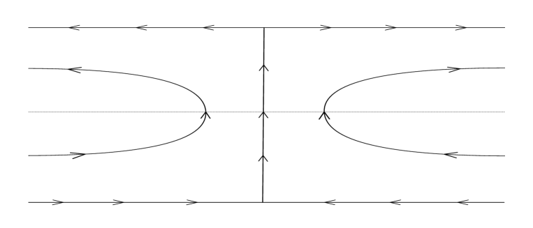
Then solves the elliptic equation in (54) in . Denote . Note that is bounded by a standard gradient estimate. Then is a bounded and smooth solution to the Euler system (1) in satisfying the slip boundary condition (2). It follows from Theorem 1.2 (ii) and (55) that must be of Type III. Note that by uniqueness, is symmetric with respect to the line . Moreover, by [13, Lemma 6], converges to a shear flow uniformly for (resp. ) in bounded intervals as (resp. ). Incorporating all the information and remembering (55) and (59), the Type III flow constructed above exhibits streamlines shown in Figure 1. This flow has exactly one stagnation point, which is also a saddle point of streamlines, located at the origin.

Obviously, by an odd reflection about the -axis, the solution defined in (61) can be further extended to an entire solution to (54) in . Such a solution is called a saddle solution with four ends, which is a special case of the so-called finite-end solutions. Roughly speaking, an end is a direction toward which the flow converges to a shear flow. For more studies on the existence, qualitative properties, and classification of finite-end solutions to the Allen-Cahn equation in two-dimensional case, one may refer to [1, 14, 15, 26, 27, 28, 34, 35, 36, 37, 45] and references therein.
6.3. Existence of Type-III flows in a strip
We shall construct the stream function of a Type III flow in by solving a bounded solution to the problem
| (62) |
In this subsection, let satisfy
| (63) |
together with
| (64) |
A typical example of such functions is with .
The restriction of a solution to (62) to is a positive solution to (54) in . Conversely, given a positive solution of the problem (54) in . If we extend to be via the extension in (61) with replaced by and still denote by , then is a solution to (62).
We shall use the method of sub- and supersolutions to construct a positive and bounded solution to (54) in . In the following, a substantial portion of our argument is standard and can be located in references such as [6, 7, 13]. Nevertheless, for the reader’s convenience, we provide essential elaborations in our proof.
We start with the existence and uniqueness of a one-dimensional solution.
Lemma 6.2.
Proof.
Since and , for sufficiently small, one has for all . Hence for the same , the function satisfies
Therefore, is a subsolution to the problem (65). Note that . So for every , is a supersolution. Now for small, we have in . Then by the method of sub- and supersolutions (see, e.g., [19]), there exists a solution satisfying in . Obviously, is positive in .
Assume is also a positive solution. Then the function is a subsolution. Let be so large that in . Then there exists a third positive solution between and . Using the elliptic equation and integrating by part yield
Since in , and is strictly decreasing, we conclude that . Similarly, we have . This completes the proof. ∎
In what follows, for , we denote and the open rectangles and , respectively.
Lemma 6.3 (Existence).
There exists a bounded solution to (62).
Proof.
First, the one-dimensional solution constructed in Lemma 6.2 is a supersolution to (54) in . Next, we need to construct a nonnegative subsolution. Note that there exists a small positive number such that
So for small, it holds that
Define
| (66) |
where and (it suffices to choose in this proof, but we need to choose large enough in the proof of uniqueness later). The straightforward computations yield that , and
It is easy to see the outer normal derivative on . Therefore, for every with , it holds that
Hence is a weak subsolution to (54) in . By our construction, it is easily seen that in provided is small enough, where is the solution of (65) established in Lemma 6.2.
Now for every with , and are still sub- and supersolutions to (54) in . So there exists a weak solution to (54) in such that in . By the standard regularity theory for elliptic equations (cf. [24]), is regular up to the boundary except possibly at the corners of . Since is an odd function, the odd extension of with respect to , denoted by , is a solution to (54) in . Hence for any , it follows again from the regularity theory for elliptic equations that
where is a constant depending on but independent of . By the Arzelá–Ascoli theorem and Cantor’s diagonal argument, (up to a subsequence) converges to some limit in on any compact subsets of . Hence is a bounded solution to (54) in and is odd in . Since in and is nontrivial, the strong maximum principle implies that must be positive in . Therefore, solves (62). This completes the proof of the lemma. ∎
Lemma 6.4 (Asymptotics).
Proof.
First, the restriction of to is a positive and bounded solution to (54) in . Thanks to (56), there exists a bounded function, , defined by
Obviously, is positive in and .
For , define for . It follows from the regularity theory for elliptic equations that for any , one has
Hence by the Arzelá–Ascoli theorem and the existence of , converges to the function in as . Since solves
letting implies that is a positive solution to (65). It then follows from Lemma 6.2 that . This completes the proof of the lemma. ∎
Lemma 6.5 (Uniqueness).
There exists a unique bounded solution to (62). Moreover, this unique solution is odd in .
Proof.
The existence has been proved in Lemma 6.3.
Let be two bounded solutions to (62). Then is a positive supersolution to (54) in . Recall the subsolution defined by (66). In view of (67), one can choose so large that in . Following the proof of Lemma 6.3, there exists a bounded solution to (62) such that
Now for every , we have
Since in and is strictly decreasing, it holds that
Letting and recalling (67) give
This implies in . Similarly, in , and thus, in .
Now the functions and are also bounded solutions to (62). By the previous step, we have
Hence the lemma immediately follows. ∎
Incorporating (56), (57), (58), (60), Lemma 6.4 and Lemma 6.5, we arrive at the following proposition.
Proposition 6.6.
There exists a unique bounded solution to (62). Moreover, this unique solution satisfies that
(i) for all ;
(ii) in , and in ;
(iii) uniformly in .
Finally, assuming is smooth and introducing , we prove the following proposition.
Proposition 6.7.
There exists a bounded solution to the Euler system in satisfying and the following properties.
-
(a)
for all , and in ;
-
(b)
for all , and in ;
-
(c)
uniformly in .
This Type III flow exhibits streamlines shown in Figure 2. There are exactly two stagnation points located at and .
Acknowledgement. The research of Gui is supported by University of Macau research grants CPG2024-00016-FST, SRG2023-00011-FST, UMDF Professorial Fellowship of Mathematics, and Macao SAR FDCT 0003/2023/RIA1. The research of Xie is partially supported by NSFC grants 12250710674 and 11971307, the Fundamental Research Funds for the Central Universities, Natural Science Foundation of Shanghai 21ZR1433300, and Program of Shanghai Academic Research Leader 22XD1421400.
References
- [1] F. Alessio, A. Calamai, and P. Montecchiari, Saddle-type solutions for a class of semilinear elliptic equations, Adv. Differential Equations, 12 (2007), no.4, 361–380.
- [2] L. Ambrosio and X. Cabré, Entire solutions of semilinear elliptic equations in and a conjecture of De Giorgi, J. Amer. Math. Soc., 13 (2000), no. 4, 725–739.
- [3] G. K. Batchelor, An introduction to fluid dynamics, Second paperback edition, Cambridge Math. Lib. Cambridge University Press, Cambridge, 1999.
- [4] H. Berestycki, L. Caffarelli, and L. Nirenberg, Inequalities for second-order elliptic equations with applications to unbounded domains I, Duke Math. J., 81 (1996), no.2, 467–494.
- [5] H. Berestycki, L. Caffarelli, and L. Nirenberg, Further qualitative properties for elliptic equations in unbounded domains, Ann. Scuola Norm. Sup. Pisa Cl. Sci., 25 (1997), 69–94.
- [6] H. Berestycki, F. Hamel, and L. Rossi, Liouville-type results for semilinear elliptic equations in unbounded domains, Ann. Mat. Pura Appl., 4 (2007), no.3, 469–507.
- [7] H. Berestycki and P. L. Lions, Some applications of the method of super and subsolutions, Bifurcation and nonlinear eigenvalue problems (Proc., Session, Univ. Paris XIII, Villetaneuse, 1978), pp. 16–41, Lecture Notes in Math., 782 Springer, Berlin, 1980.
- [8] H. Berestycki and L. Nirenberg, On the method of moving planes and the sliding method, Bol. Soc. Brasil. Mat. (N.S.), 22 (1991), no.1, 1–37.
- [9] Á. Castro and D. Lear, Traveling waves near Couette flow for the 2D Euler equation, Comm. Math. Phys., 400 (2023), no.3, 2005–2079.
- [10] O. Chodosh and C. Li, Stable minimal hypersurfaces in , to appear in Acta Mathematica.
- [11] P. Constantin, T. D. Drivas, D. Ginsberg, Flexibility and rigidity in steady fluid motion, Comm. Math. Phys., 385 (2021), no.1, 521–563.
- [12] M. Coti Zelati, T. Elgindi, and K. Widmayer, Stationary structures near the Kolmogorov and Poiseuille flows in the 2d Euler equations, Arch. Ration. Mech. Anal., 247 (2023), no.1, Paper No. 12, 37 pp.
- [13] H. Dang, P. C. Fife, and L. A. Peletier, Saddle solutions of the bistable diffusion equation, Z. Angew. Math. Phys., 43 (1992), no.6, 984–998.
- [14] M. del Pino,, M. Kowalczyk, and F. Pacard, Moduli space theory for the Allen-Cahn equation in the plane, Trans. Amer. Math. Soc., 365 (2013), no.2, 721–766.
- [15] M. del Pino, M. Kowalczyk, F. Pacard, and J. Wei, Multiple-end solutions to the Allen-Cahn equation in , J. Funct. Anal., 258 (2010), no.2, 458–503.
- [16] S. A. Denisov, Infinite superlinear growth of the gradient for the two-dimensional Euler equation, Discrete Contin. Dyn. Syst., 23 (2009), no. 3, 755–764.
- [17] P. G. Drazin and W. H. Reid, Hydrodynamic stability, Second edition, Cambridge University Press, Cambridge, 2004.
- [18] T. M. Elgindi and Y. Huang, Regular and Singular Steady States of 2D incompressible Euler equations near the Bahouri-Chemin Patch, arXiv:2207.12640.
- [19] L. C. Evans. Partial differential equations, Second edition, American Mathematical Society, 2010.
- [20] L. C. Evans, R. F. Gariepy, Measure theory and fine properties of functions, Stud. Adv. Math. CRC Press, Boca Raton, FL, 1992.
- [21] L. Franzoi, N. Masmoudi, and R. Montalto, Space quasi-periodic steady Euler flows close to the inviscid Couette flow, arXiv: 2303.03302.
- [22] N. Ghoussoub and C. Gui, On a conjecture of De Giorgi and some related problems, Math. Ann., 311 (1998), no. 3, 481–491.
- [23] B. Gidas, W. M. Ni, and L. Nirenberg, Symmetry and related properties via the maximum principle, Comm. Math. Phys., 68 (1979), no.3, 209–243.
- [24] D. Gilbarg and N. Trudinger. Elliptic partial differential equations of second order, 2nd Ed., Springer-Verlag, Berlin, 1983.
- [25] J. Gómez-Serrano, J. Park, J. Shi, and Y. Yao, Symmetry in stationary and uniformly rotating solutions of active scalar equations, Duke Math. J., 170 (2021), no.13, 2957–3038.
- [26] C. Gui, Hamiltonian identities for elliptic partial differential equations, J. Funct. Anal., 254 (2008), no.4, 904–933.
- [27] C. Gui, Symmetry of some entire solutions to the Allen-Cahn equation in two dimensions, J. Differential Equations, 252 (2012), no.11, 5853–5874.
- [28] C. Gui, Y. Liu, and J. Wei, On variational characterization of four-end solutions of the Allen-Cahn equation in the plane, J. Funct. Anal., 271 (2016), no.10, 2673–2700.
- [29] F. Hamel and N. Nadirashvili, Shear flows of an ideal fluid and elliptic equations in unbounded domains, Comm. Pure Appl. Math., 70 (2017), 590–608.
- [30] F. Hamel and N. Nadirashvili, A Liouville theorem for the Euler equations in the plane, Arch. Ration. Mech. Anal., 233 (2019), 599–642.
- [31] F. Hamel and N. Nadirashvili, Circular flows for the Euler equations in two-dimensional annular domains, and related free boundary problems, J. Eur. Math. Soc., 25 (2023), no.1, 323–368.
- [32] G. Luo and T. Y. Hou, Formation of finite-time singularities in the 3D axisymmetric Euler equations: a numerics guided study, SIAM Rev., 61 (2019), no. 4, 793–835.
- [33] A. Kiselev and V. Sverak, Small scale creation for solutions of the incompressible two-dimensional Euler equation, Ann. of Math., 180 (2014), no. 3, 1205–1220.
- [34] M. Kowalczyk, Y. Liu, and F. Pacard, The space of 4-ended solutions to the Allen-Cahn equation in the plane, Ann. Inst. H. Poincaré C Anal. Non Linéaire, 29 (2012), no.5, 761–781.
- [35] M. Kowalczyk, Y. Liu, and F. Pacard, Towards classification of multiple-end solutions to the Allen-Cahn equation in , Netw. Heterog. Media, 7 (2012), no.4, 837–855.
- [36] M. Kowalczyk, Y. Liu, and F. Pacard, The classification of four-end solutions to the Allen-Cahn equation on the plane, Anal. PDE, 6 (2013), no.7, 1675–1718.
- [37] M. Kowalczyk, Y. Liu, F. Pacard, and J. Wei, End-to-end construction for the Allen-Cahn equation in the plane, Calc. Var. Partial Differential Equations, 52 (2015), no.1-2, 281–302.
- [38] C. Li, Y. Lü, H. Shahgholian, and C. Xie, Steady solutions for the Euler system in an infinitely long nozzle, arXiv: 2203.08375.
- [39] Z. Lin and C. Zeng, Inviscid dynamical structures near Couette flow, Arch. Ration. Mech. Anal., 200 (2011), no.3, 1075–1097.
- [40] N. Nadirashvili, On stationary solutions of two-dimensional Euler equation, Arch. Ration. Mech. Anal., 209 (2013), no.3, 729–745.
- [41] D. Ruiz, Symmetry results for compactly supported steady solutions of the 2D Euler equations, Arch. Ration. Mech. Anal., 247 (2023), no.3, Paper No. 40, 25 pp.
- [42] R. Schoen, Estimates for stable minimal surfaces in three-dimensional manifolds. Seminar on minimal submanifolds, 111–126. Ann. of Math. Stud., 103 Princeton University Press, Princeton, NJ, 1983
- [43] R. Schoen, L. Simon, and S. T. Yau, Curvature estimates for minimal hypersurfaces, Acta Math., 134 (1975), no.3-4, 275–288.
- [44] J. Simons, Minimal varieties in riemannian manifolds, Ann. of Math., 88 (1968), 62–105.
- [45] K. Wang and J. Wei, Finite Morse index implies finite ends, Comm. Pure Appl. Math., 72 (2019), no.5, 1044–1119.
- [46] Y. Wang and W. Zhan, On the rigidity of the 2D incompressible Euler equations, arXiv: 2307.00197