Stacking Your Transformers: A Closer Look at Model Growth for Efficient LLM Pre-Training
Abstract
LLMs are computationally expensive to pre-train due to their large scale. Model growth emerges as a promising approach by leveraging smaller models to accelerate the training of larger ones. However, the viability of these model growth methods in efficient LLM pre-training remains underexplored. This work identifies three critical Obstacles: (O1) lack of comprehensive evaluation, (O2) untested viability for scaling, and (O3) lack of empirical guidelines. To tackle O1, we summarize existing approaches into four atomic growth operators and systematically evaluate them in a standardized LLM pre-training setting. Our findings reveal that a depthwise stacking operator, called , exhibits remarkable acceleration in training, leading to decreased loss and improved overall performance on eight standard NLP benchmarks compared to strong baselines. Motivated by these promising results, we conduct extensive experiments to delve deeper into to address O2 and O3. For O2 (untested scalability), our study shows that is scalable and consistently performs well, with experiments up to 7B LLMs after growth and pre-training LLMs with 750B tokens. For example, compared to a conventionally trained 7B model using 300B tokens, our model converges to the same loss with 194B tokens, resulting in a 54.6% speedup. We further address O3 (lack of empirical guidelines) by formalizing guidelines to determine growth timing and growth factor for , making it practical in general LLM pre-training. We also provide in-depth discussions and comprehensive ablation studies of . Our code and pre-trained model are available at https://llm-stacking.github.io/.
1 Introduction
Emergent abilities of Large Language Models (LLMs) rely on scaling-up [1, 2]. Empirical evidence from scaling laws [3, 4, 5] fuels the development of increasingly larger models, pushing the boundaries of LLMs capabilities. However, pre-training these gigantic models comes at a significant cost in terms of energy consumption and environmental impact [6] (e.g., pre-training Llama-3 [7] consumes a total of 7.7M GPU hours and generates 2290 tons of carbon dioxide equivalent of carbon emissions). The efficient pre-training of LLMs is thus crucial, both from a scientific and a societal perspective, to ensure the continual growth and adoption of AI [8, 9].
One promising research direction to accelerate model training involves leveraging trained smaller (base) models to expedite the training of larger (target) models, a technique known as model growth. Concretely, model growth studies how to leverage the trained smaller model’s parameters to initialize the larger model’s parameters . The primary objective is to accelerate the training of large models, and existing methods demonstrate promising speedup results on models such as BERT [10, 11, 12, 13, 14, 15]. Despite such empirical evidence and its alignment with the goal of efficient LLM pre-training, model growth methods are not widely adopted in the context of LLM pre-training [7, 16]. To our best knowledge, the only LLM that utilizes model growth for accelerating is FLM-101B [17], but it lacks a baseline LLM trained from scratch to compare. We observe three key Obstacles that hinder LLM pre-training from using existing model growth techniques, specifically:
O1: Lack of comprehensive assessment. Some existing model growth methods report results on LLM pre-training, but either lack a baseline comparison [17] or are still in exploratory stages [13, 15]. In contrast, most growth approaches are evaluated in encoder-based BERT models [11, 10, 12, 14, 15, 18, 19], which have different architecture and training configurations compared to prominent decoder-based LLMs such as Llama [20].
O2: The untested scalability. This scalability has two aspects: the model size and the amount of pre-training data. Regarding the model size, the existing approaches are only evaluated on smaller-scale BERT models or in preliminary experiments with LLMs. It is unclear whether these growth methods will continue accelerating training when applied to large-scale LLMs with more extensive evaluation. As for the amount of pre-training data, there are debates [21] over whether certain efficient training strategies may initially converge faster but ultimately perform similarly or worse than vanilla training methods when given ample computational resources (i.e., more training data).
O3: Lack of empirical guidelines. Scaling laws [3, 4] give clear empirical guidelines on pre-training computational-optimized LLMs, greatly stimulating and advancing the field. Yet, there is a lack of empirical guidelines on growth techniques, discouraging LLM practitioners from adopting these approaches, especially considering the high costs of LLM pre-training.
These three obstacles are consequential in nature. Hence, in this work, we empirically revisit the concept of model growth as a solution to efficient LLM pre-training by tackling them one by one.
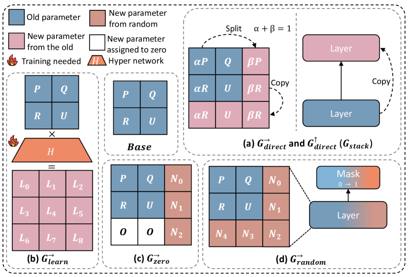
To tackle O1, we systematically evaluate model growth techniques on practical LLM pre-training. We first categorize existing growth methods and summarize them into four atomic growth operators, each of which can grow along two directions: widthwise (intra-layer) and depthwise (layer-wise). We illustrate them in Figure 2. These operators serve as representative choices for evaluating the performance of model growth techniques. We use these operators to expand 400M base models to 1.1B Llama-like LLMs and continually pre-train them. Next, we evaluate these growth techniques on the training loss and eight standard NLP benchmarks from the Harness toolkit [22]. We found the direct operator that stacks depthwisely consistently outperforms others across overall evaluation metrics, demonstrating its potential in accelerating LLM pre-training. This motivates us to investigate extensively by addressing O2 and O3 on .
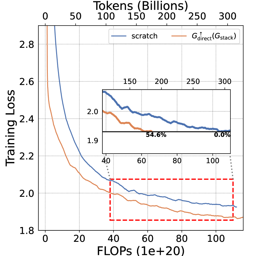
To address O2, we investigate the operator’s scalability to larger model sizes and to more training data. We conduct extensive experiments by scaling model size up to 7B parameters trained with 300B tokens, and pre-training a 410M model with over 750B training tokens. This is in contrast to the previous largest LLM pre-training experiment that uses model growth methods and has baselines for comparison, which is reported in Ligo [13], where a GPT2-1.5B model is trained for 15k steps (approximately 15B tokens). The results are encouraging, as we consistently observe significant improvements offers in both scenarios. For example, we achieve a remarkable 54.6% speedup in pre-training for a 7B model with 300B tokens (Figure 1). Interestingly, the loss improvement in our 750B-token experiment aligns with a logarithmic function. We further extend this logarithmic curve and determine that the improvement continues to be substantial even for the LLM trained with over 8T tokens. Moreover, we summarize all our experiments by estimating the LLM scaling law for LLMs pre-trained with . Given the same target loss value, our analysis reveals a significantly reduced computational cost compared to the common scaling law [4].
For O3, we explore the practical guidelines for using in LLM pre-training. Given a computational budget, we determine the optimal strategy for two key factors of , growth timing and growth factor . Growth timing relates to the training tokens used for small models before growing, and growth factor refers to the factor between the non-embedding parameter number of the large models and the small models. We formalize our findings into equations that offer concrete suggestions for utilizing . We believe this work could significantly pique the interest and bolster confidence in future LLM pre-training with model growth techniques, both in academia and industry.
To summarize, our contributions are four-fold: 1) We first systematically investigate model growth techniques and identify four atomic model growth operators, establishing a better understanding of the field in Section 3.1. 2) We then design a standard LLM pre-training testbed and perform comprehensive evaluations on these operators, finding that a simple depthwise stacking exhibits significant superiority in Section 3. 3) We further demonstrate the scalability of with experiments on LLMs ranging from 410M to 7B parameters and up to 750B training tokens in Section 4.1. 4) We also provide guidelines of equations on determining growth timing and growth factors for optimal use of in Section 4.2.
2 Related Work - Model Growth for Efficient Pre-training
The idea of growing neural networks dates back to the 1990s [23, 24, 25]. The pioneering work of Net2Net [26] marks a milestone, for the first attempt to study model growth in deep learning era. Net2Net expands width and depth while keeping original functions (namely function preserving) via randomly splitting old neurons and injecting new identity layers. The widthwise splitting method of Net2Net represents a series of works that aim to “expand” the existing neurons to the desired larger size. Bert2Bert [10] serves as a BERT-based extension of the widthwise Net2Net. StagedGrow[15] doubles the width by concatenating two identical layers and halves final loss to keep function-preserving. Lemon [14] suggests integrating a parameter into the splitting of neurons in Bert2Bert, aiming to break weight symmetry. Depthwisely, StackedBert [11] simply stacks duplicated layers to form a deeper model. In contrast to the above direct copy/split approaches, LiGO [13]presents a learning-based method that initializes the larger model’s parameters via learning a linear mapping from the smaller model’s parameters.
Alongside the approaches that expand existing parameters, there are works that initialize new ones without relying on existing ones. For instance, MSG [19] proposes a multi-staged growing strategy that progressively expands transformer components, where the newly grown neurons are randomly initialized using a masking mechanism to ensure function preservation. Besides, some works have assigned specific values, like zero, to the newly initialized neurons to negate their influence [18, 14].
All the above methods are primarily explored in BERT or earlier stages of LLM pre-training. On the other hand, our objective is to present the first systematic review of model growth techniques in the LLMs era. To our knowledge, FLM-101B [17] is the only existing LLM that uses the growth method [19] for accelerating billion-scale LLM pre-training. Nonetheless, this work lacks a baseline model trained from scratch, making it difficult to assess the effectiveness of the model growth technique. In contrast, we aim to provide a comprehensive study by establishing a standardized testbed to compare LLMs trained from scratch and with various growth methods in LLM pre-training.
3 Systematically Assessing Model Growth for LLM Pre-Training
Existing model growth methods [11, 10, 12, 13, 14, 15, 18, 19] are mainly evaluated on BERT [27], with limited focus on decoder-only large-scale language models such as Llama [20]. Moreover, these growth methods are often not comparable due to different training settings [11, 10, 19, 14]. Even some growth LLMs experiments are evaluated, their results are often incomplete [17, 13]. To overcome these limitations, we first summarize existing works [11, 10, 12, 13, 14, 15, 18, 19] into four atomic growth operators to represent these growth techniques. Then we build a standardized LLMs training testbed to pre-train LLMs with four growth operators on depthwise and widthwise directions and evaluate the results with both training loss and eight evaluation metrics in Harness [22].
3.1 Growing LLMs with Growth Operators
Recent years, researchers have focused on enhancing the efficiency of training large models by making use of smaller pre-existing models [26, 10, 11, 12, 13, 14, 15, 18, 19]. These state-of-the-art methods can be categorized into two distinct groups. The first group focuses on deriving new neurons from the existing ones [26, 10, 11, 14, 13], while the second group focuses on initializing new parameters separately [12, 15, 18, 19]. Drawing from these two lines of research, we summarize four atomic growth operators. These operators include: (A) directly duplicating and stacking old layers in a depthwise manner or splitting neurons in the same layer widthwisely, denoted as , (B) generating expanded parameters using a learnable mapping matrix to the existing parameters, denoted as , (C) setting the new parameters to zero, denoted as , and (D) randomly initializing the new parameters, denoted as . The illustration of four operators is shown in Figure 2. The and growth operators produce new neurons from the current ones, in contrast to and which initialize new parameters independently. For the formal definitions of the operators and the differences to the existing growth methods in design, please refer to Appendix A. Complex growth methods, such as those involving auxiliary loss or exploring training dynamics like learning rates [28, 29, 18] are interesting. But considering the high computational cost of LLM pre-training, we focus on simple, universally applicable growth operators for different LLM pre-training settings.
To make a fair comparison of the four growth operators for LLM pre-training, we define a standardized “one-hop” growth process that involves two training phases, small model training before growth and large model training after growth. We first train the small LLMs with tokens before growing. Then, we use operator to grow them to the target LLMs by a factor of for non-embedding parameters and then continual pre-training the large LLMs for tokens. Two key factors in the procedure are worth noting: the growth factor and the data for base model training , which can be interpreted as “growth timing”. We further evaluate each growth operator by separately examining in depthwise (intra-layer) growth and widthwise (layer-wise) growth . Concretely, we start with base models (400M LLMs) trained on tokens, apply the four operators in both directions to scale them up to the target size of 1.1B (approximately a growth factor of ), and then continue training for an additional tokens. 111Given growth factor , the sum of FLOPs for training and approximately equals to consumption for training large LLMs , which is the FLOPs of our baseline trained from scratch. Appendix B contains the LLM’s architecture configuration and training details.
3.2 Pre-Training 1.1B LLMs
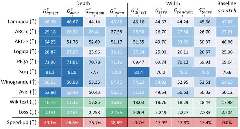
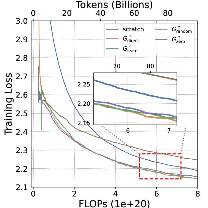
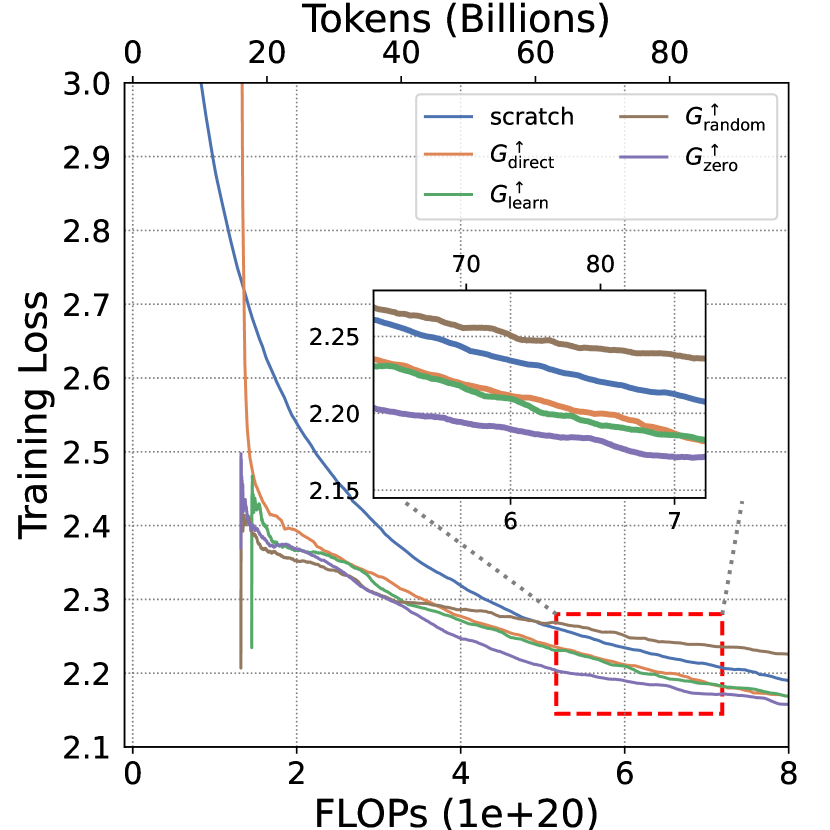
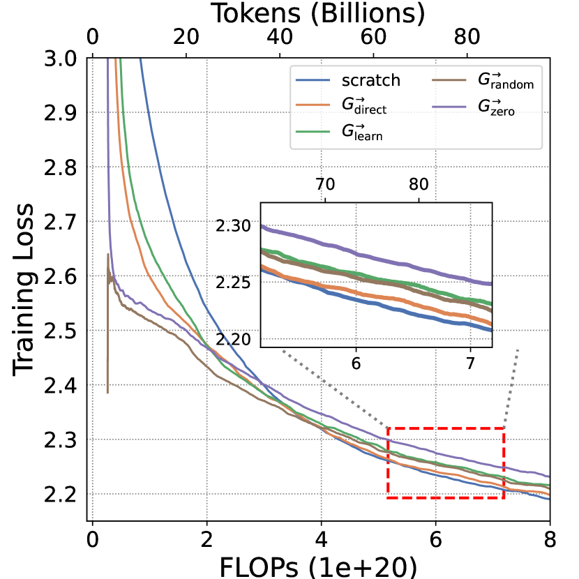
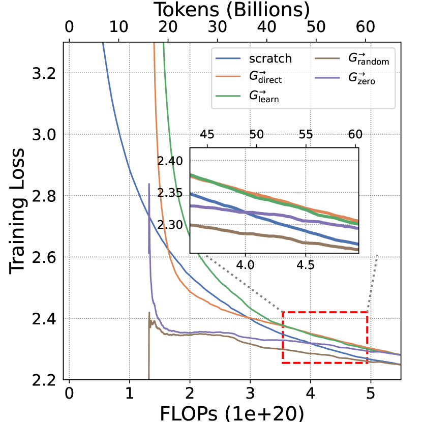
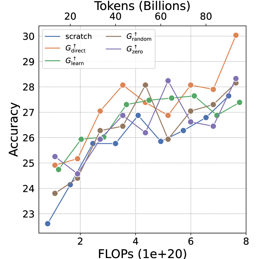
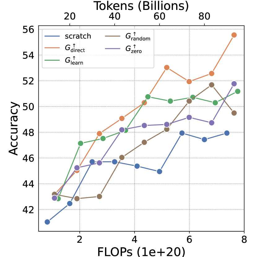
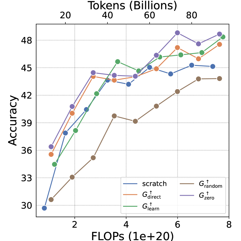
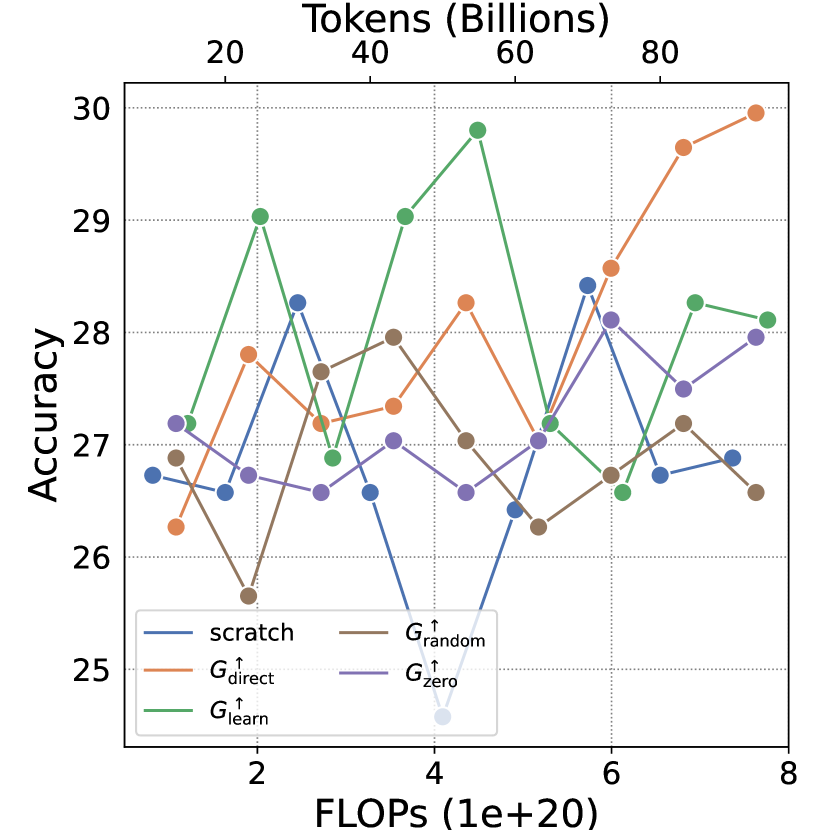
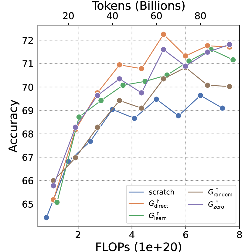
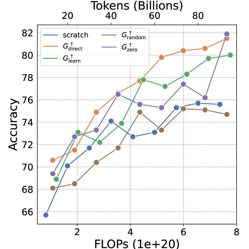
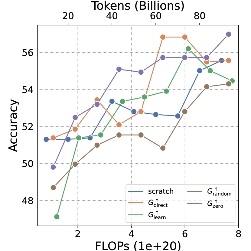
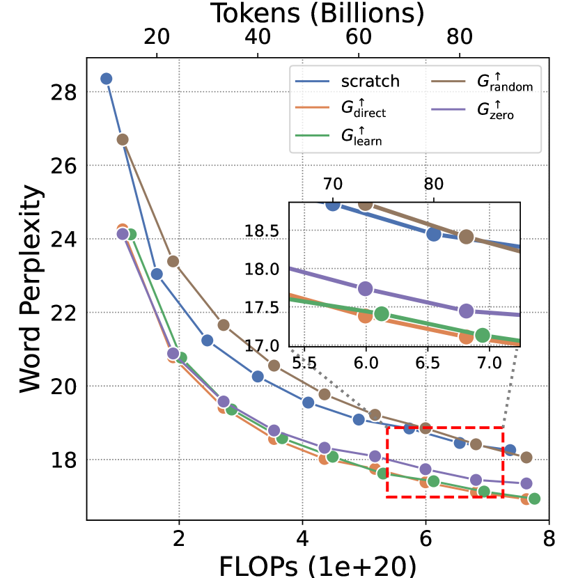
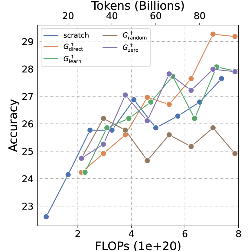
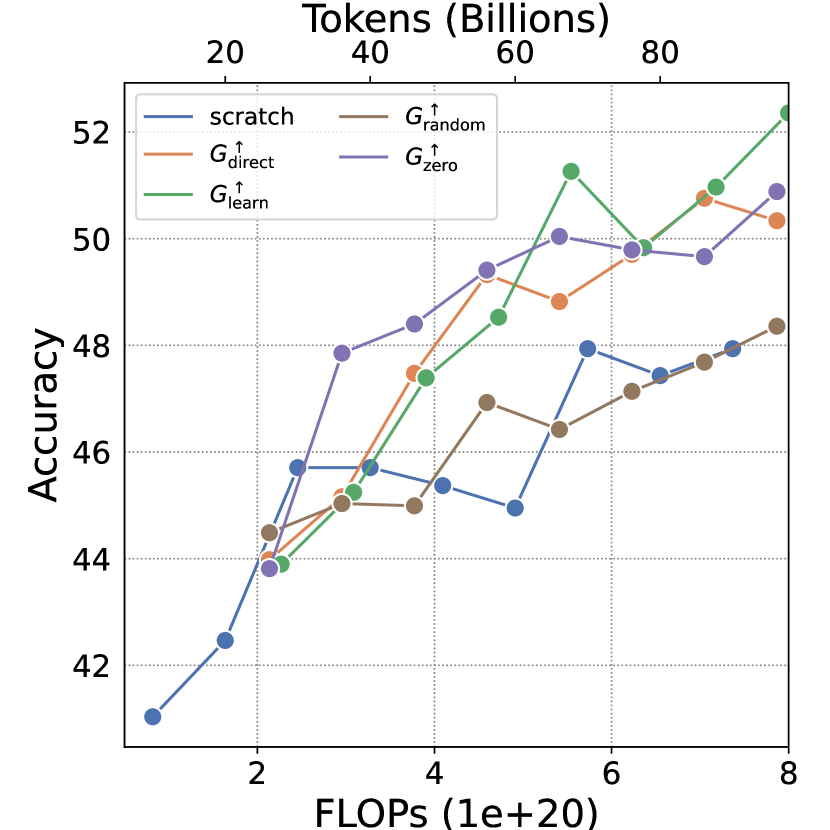
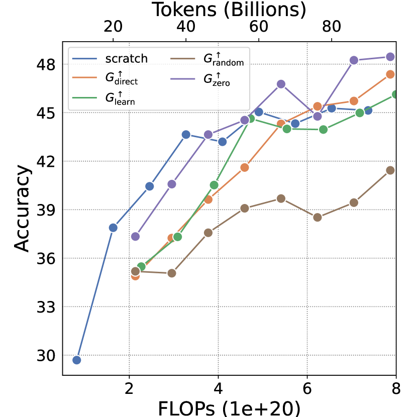
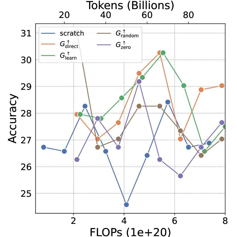
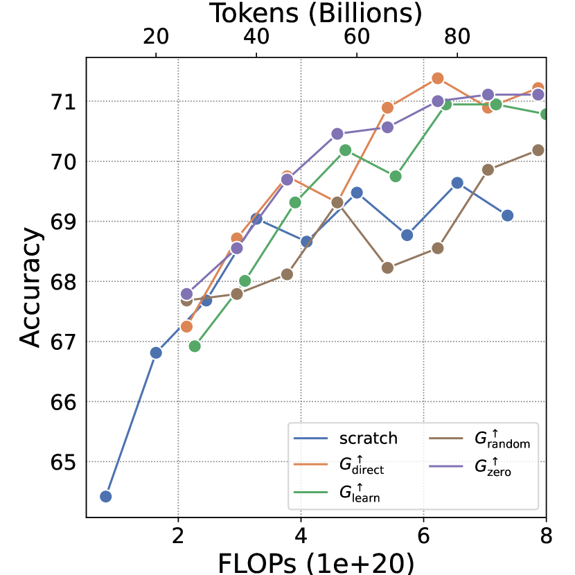
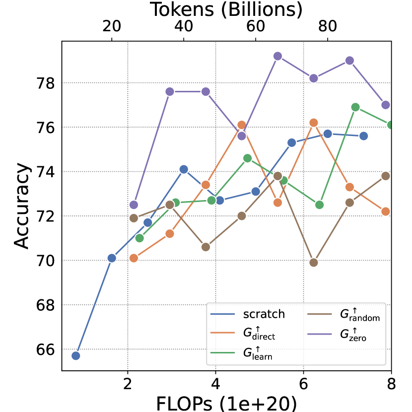
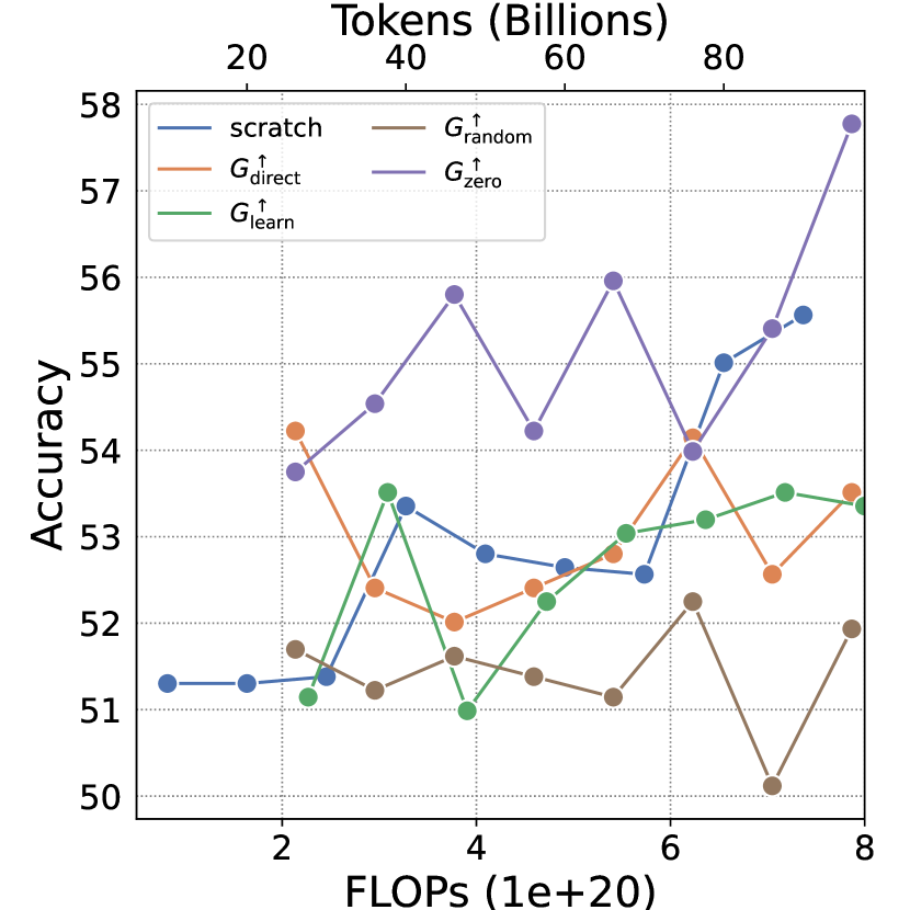
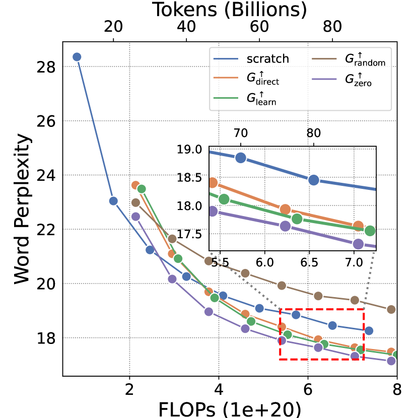
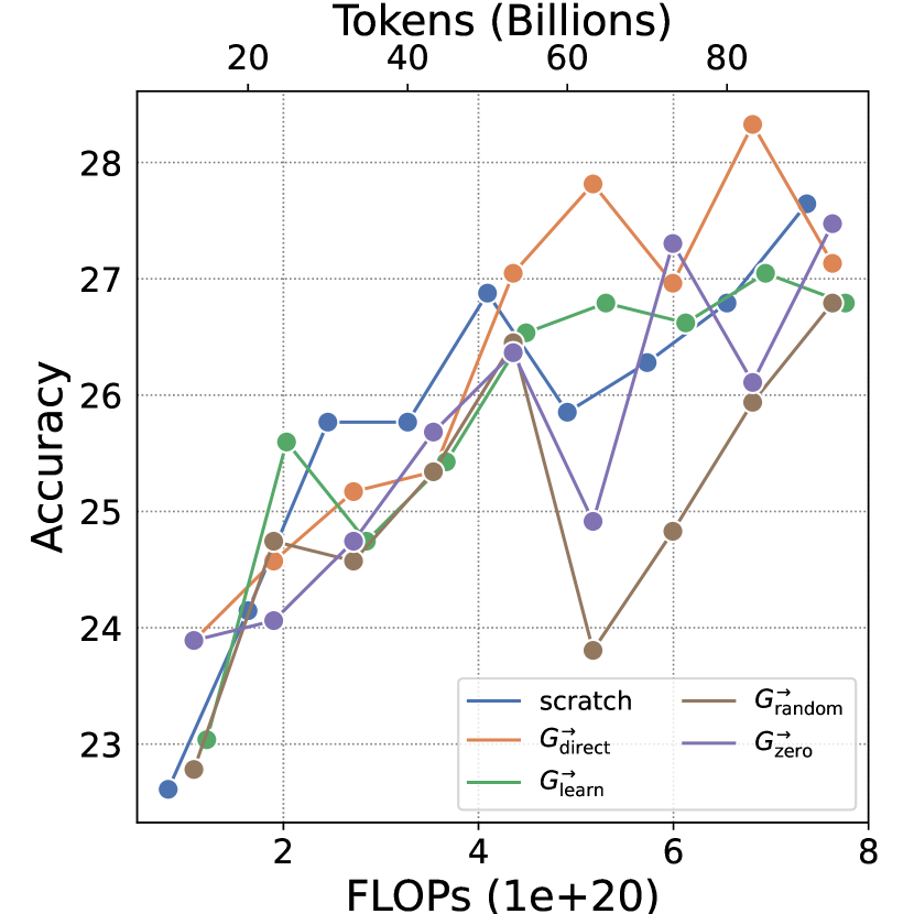
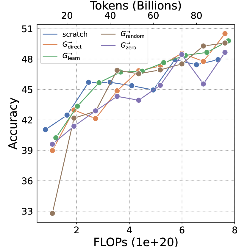
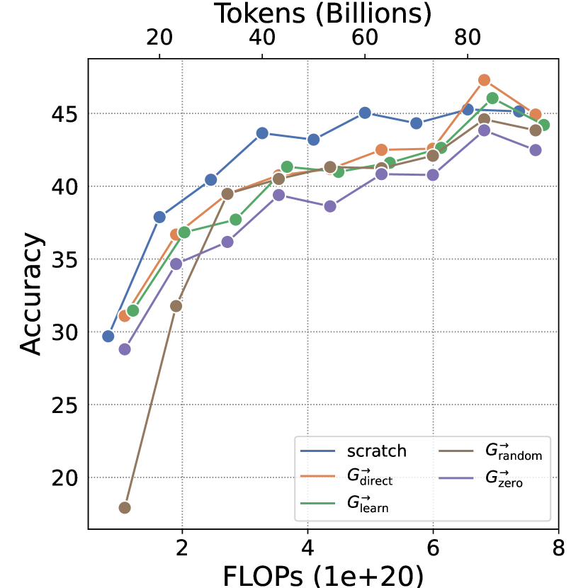
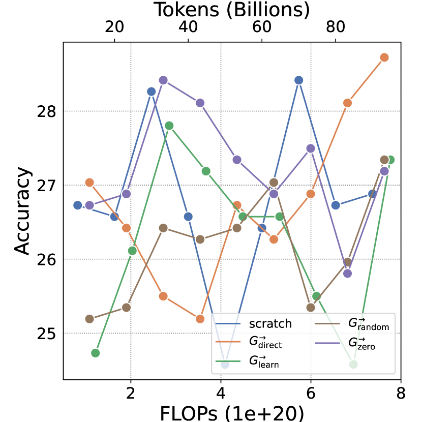
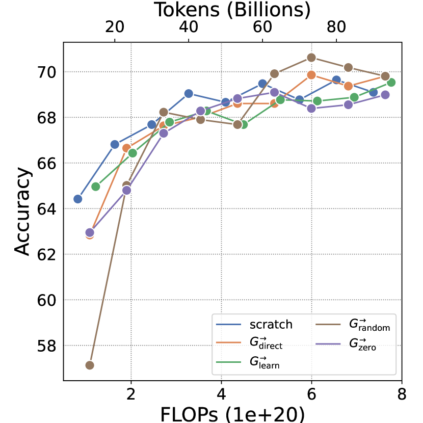
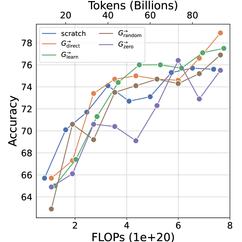
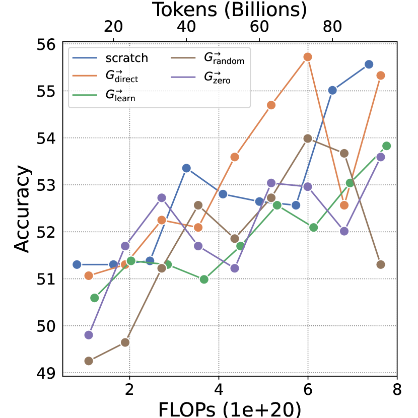
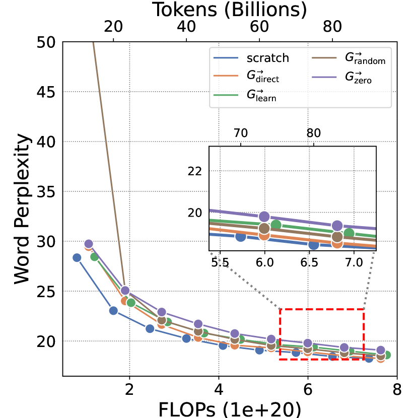
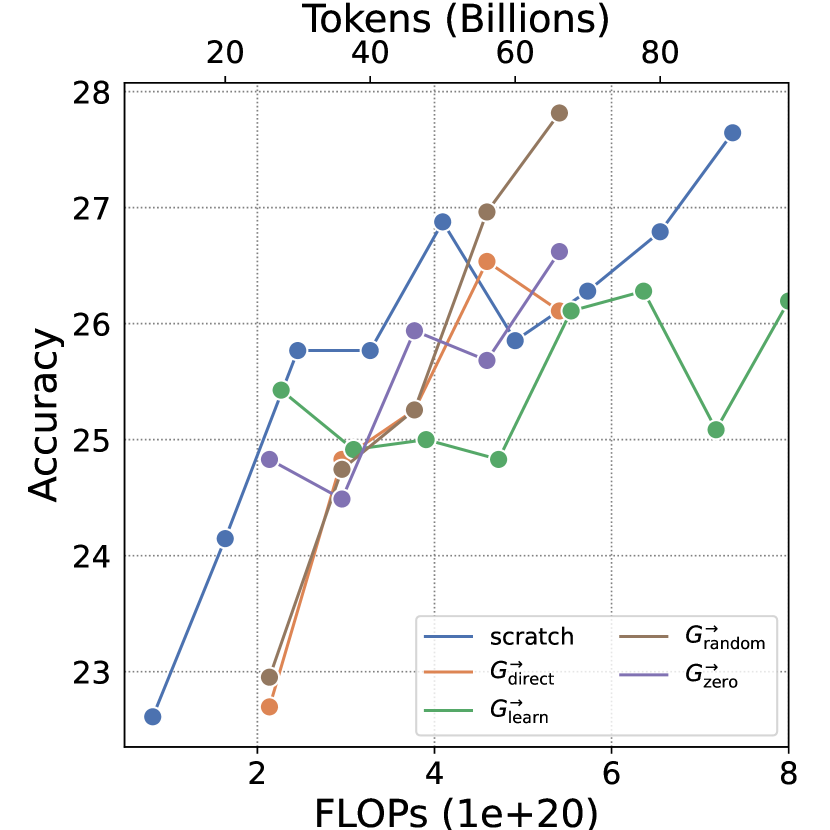
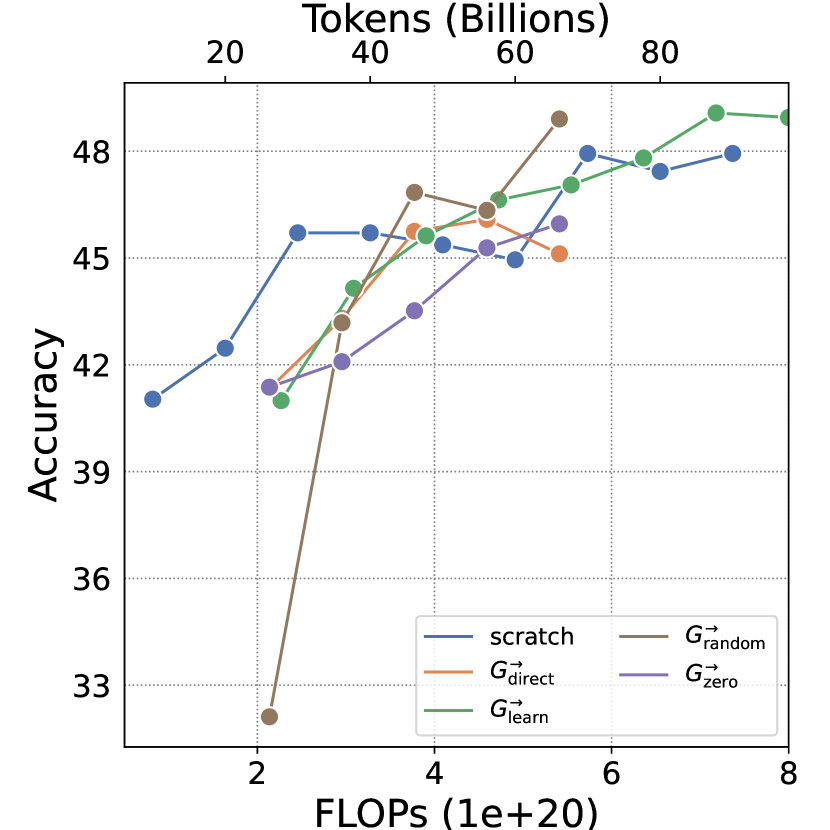
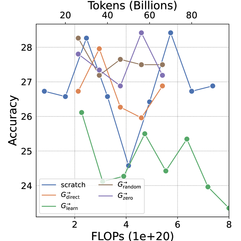
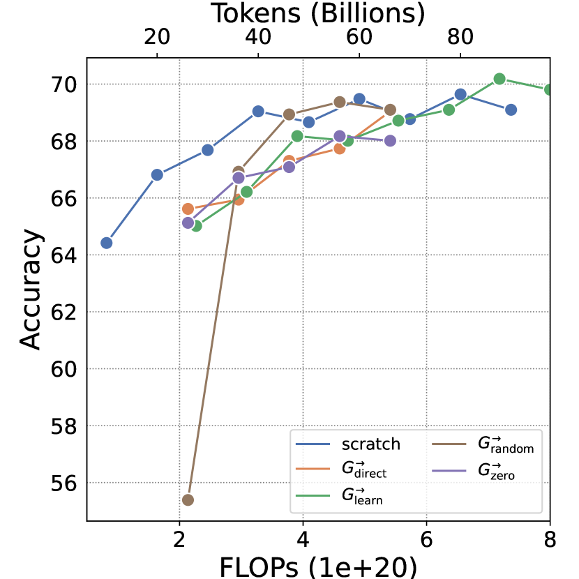
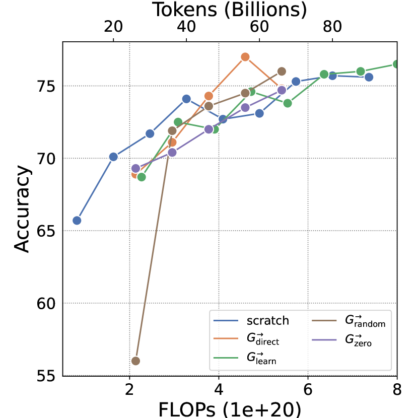
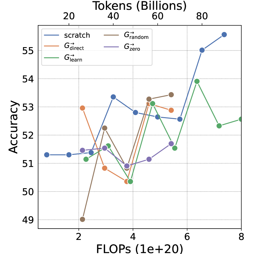
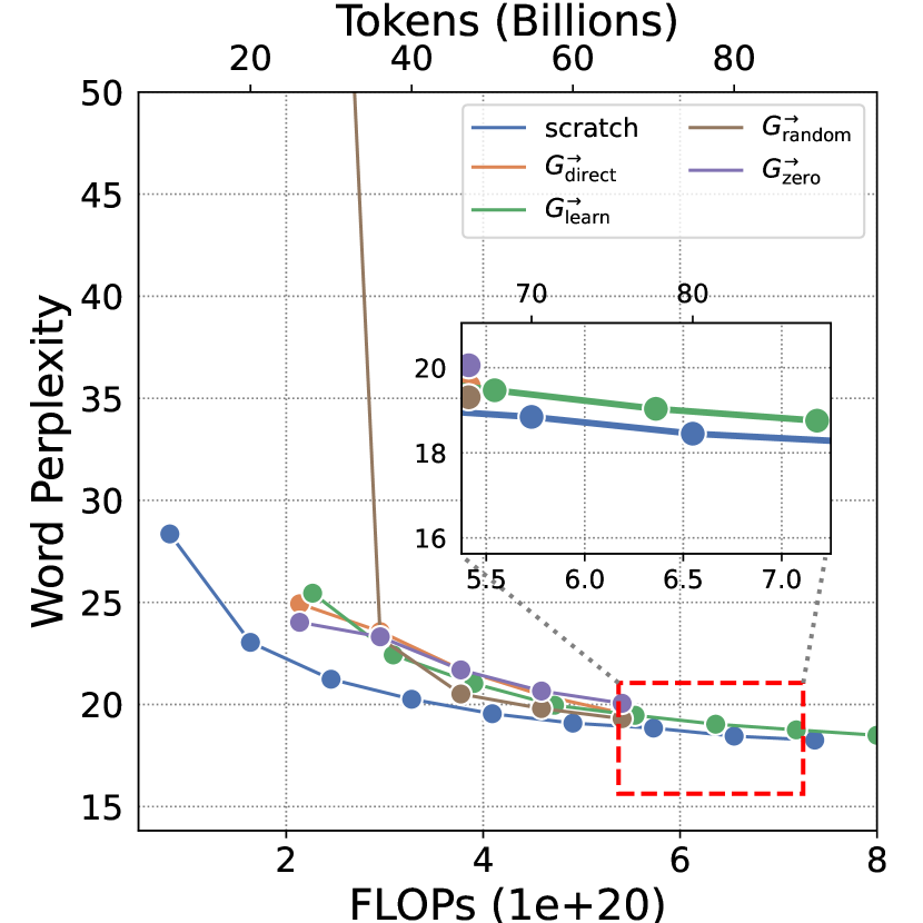
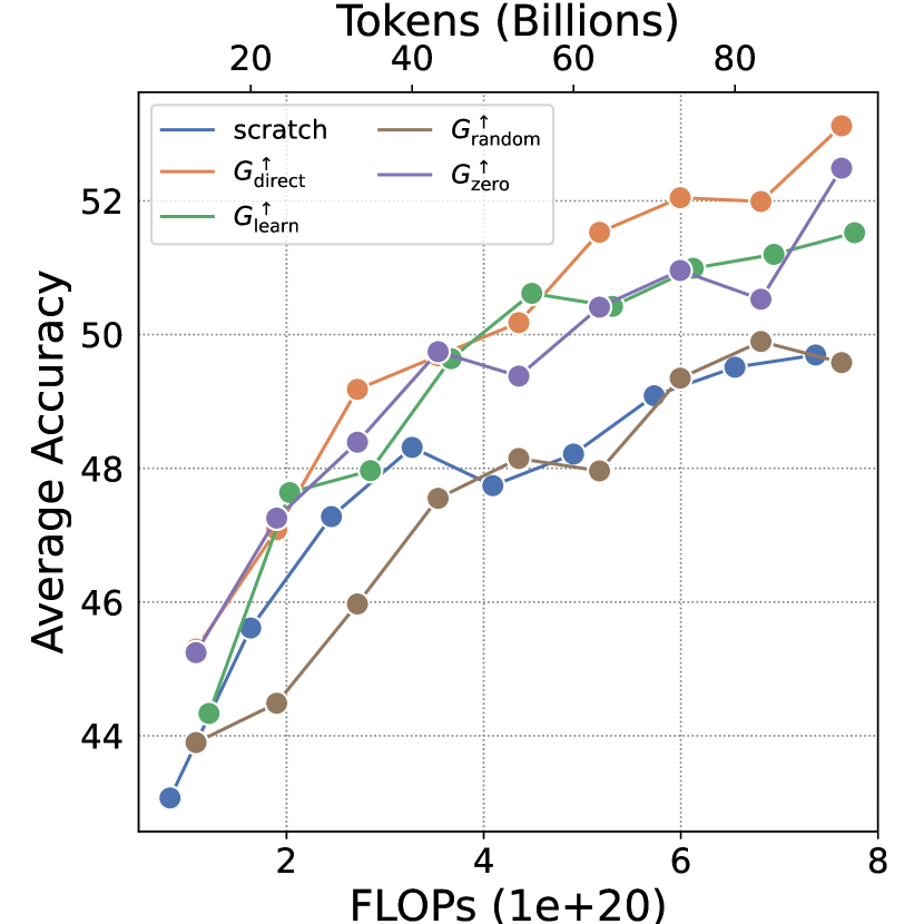
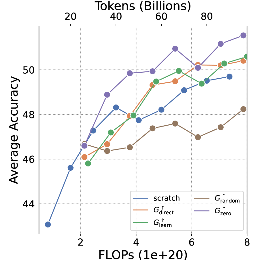
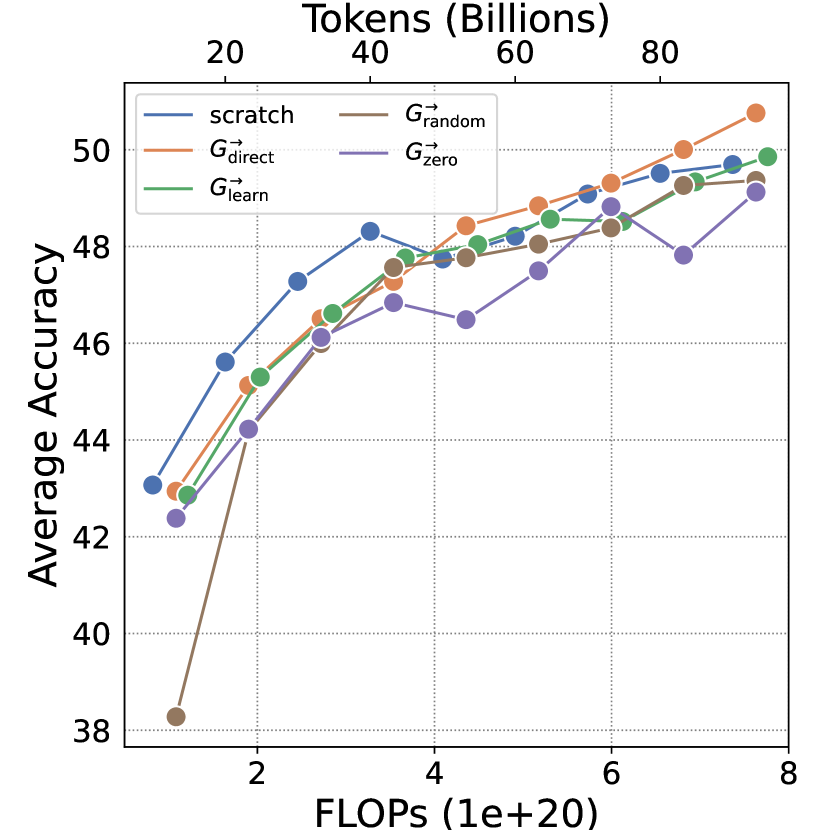
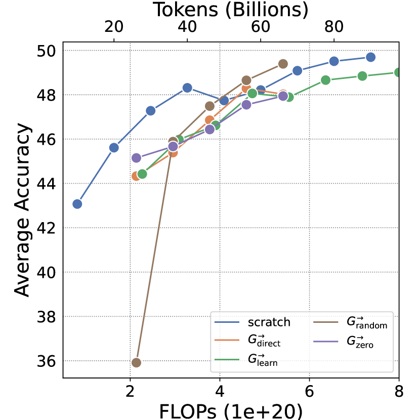
We report results on training loss, eight standard Harness NLP benchmarks along with the average accuracy and the speedup ratio in Figure 3. Our key discovery reveals that depthwise growth exhibits a significant acceleration over both widthwise growth and training models from scratch, while surprisingly, does not offer any notable advantages. Among the depthwise growth operators, , , and , all outperform the baseline and . The underperformance of in our study may be attributed to its design for gradual “mini-step” growth [19], whereas our unified approach uses a single step. Most notably, depthwise stacking emerges as the clear winner among growth operators, surpassing its competitors in speedup, training loss and nearly every Harness evaluation metric. For example, compared to training models from scratch for 100B tokens, achieves a significant efficiency gain, increasing training speed by 49.1%. The calculation of speedup please refer to Appendix B.2. The Appendix C presents more experiments on these operators, including their loss training and evaluation figures.
4 Delving Deeper Into Depthwise Stacking ()
The empirical evidence suggests that certain growth operators, most notably , exhibit an impressive acceleration in LLM pre-training compared to the baseline approach of training models from scratch. We now turn our attention to a more in-depth examination of the . For ease of reference, we will henceforth denote this depthwise stacking approach as operator : , where is a small base model trained with tokens, is the target model and is the growth factor.
This section addresses the two main challenges (O2 and O3) outlined in the introduction: 1) evaluating the performance of in scaling scenarios, i.e. larger model sizes and more training tokens; and 2) determining the hyperparameters when using , i.e., the growth timing and growth factor .
4.1 Scaling
Scaling Model Sizes for .
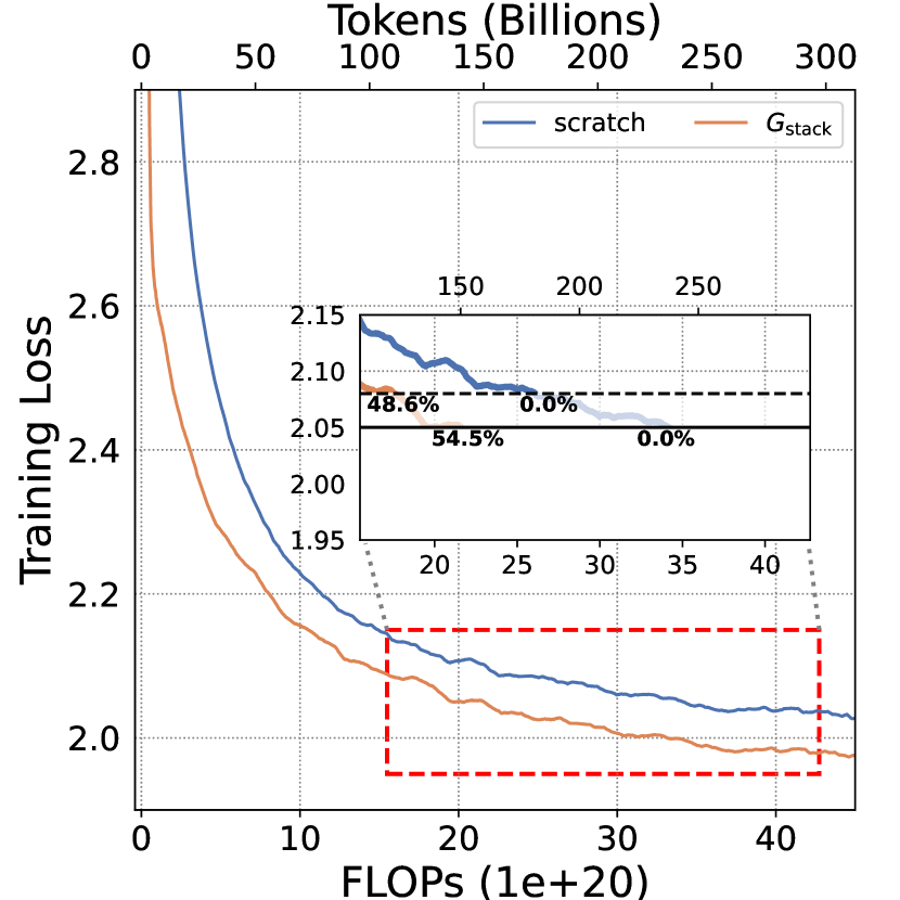
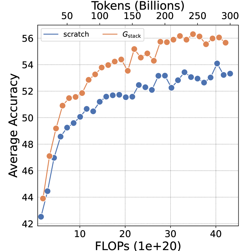
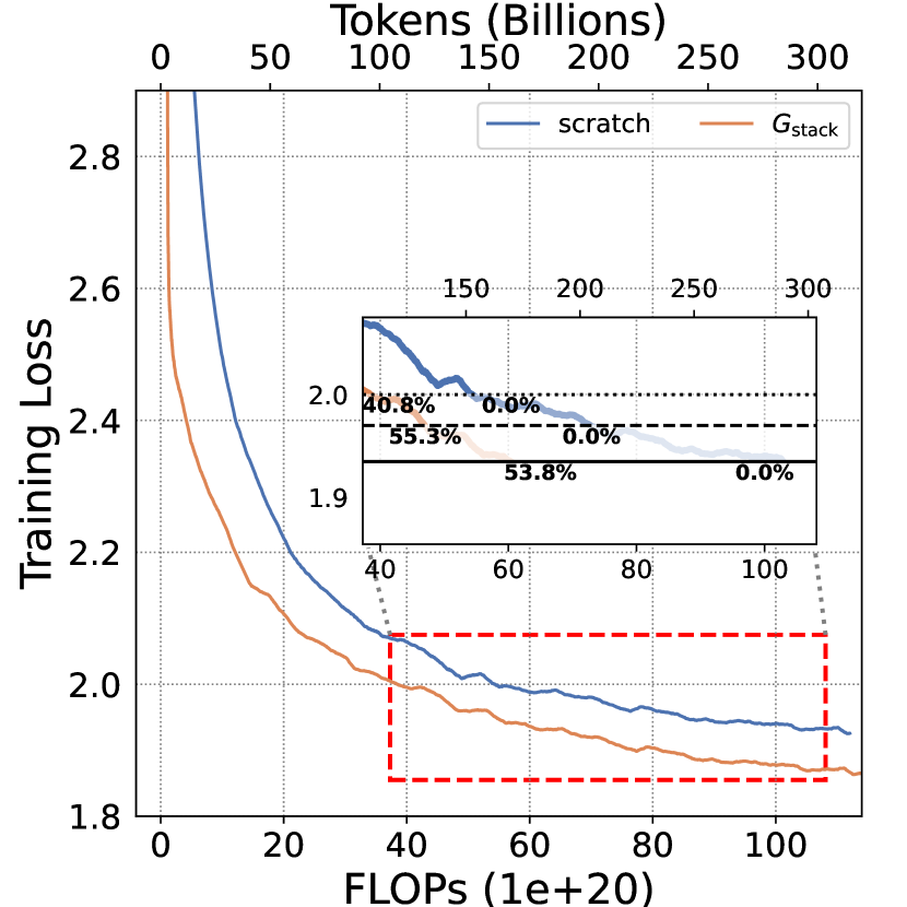
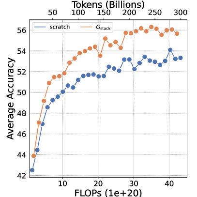
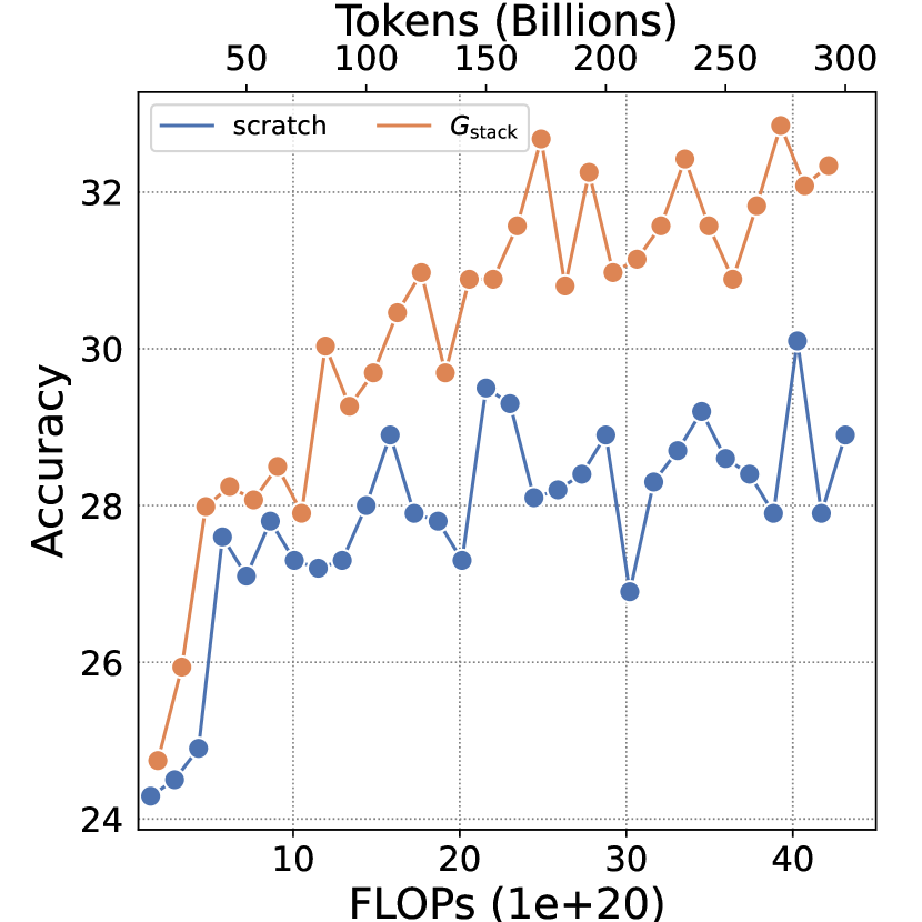
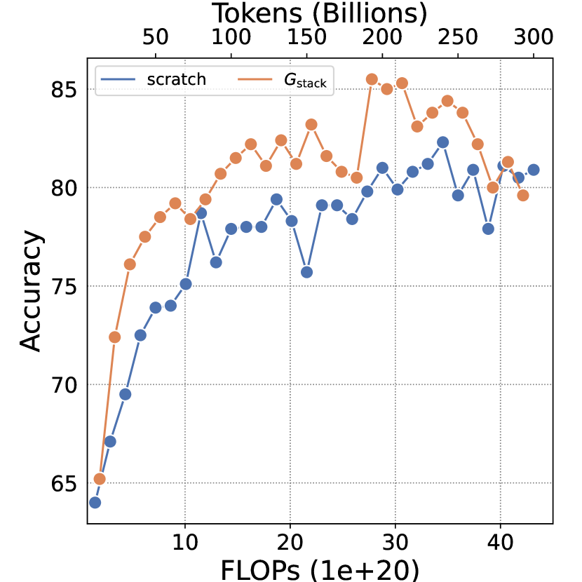
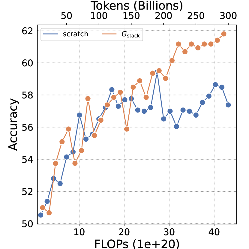
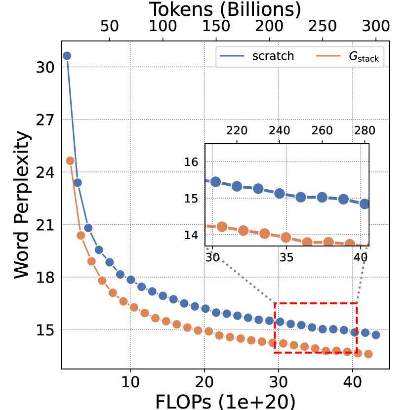
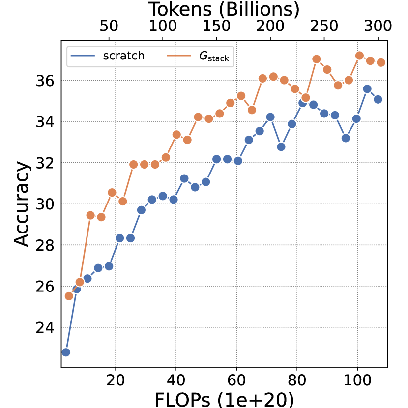
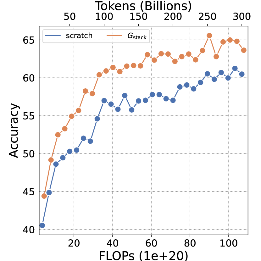
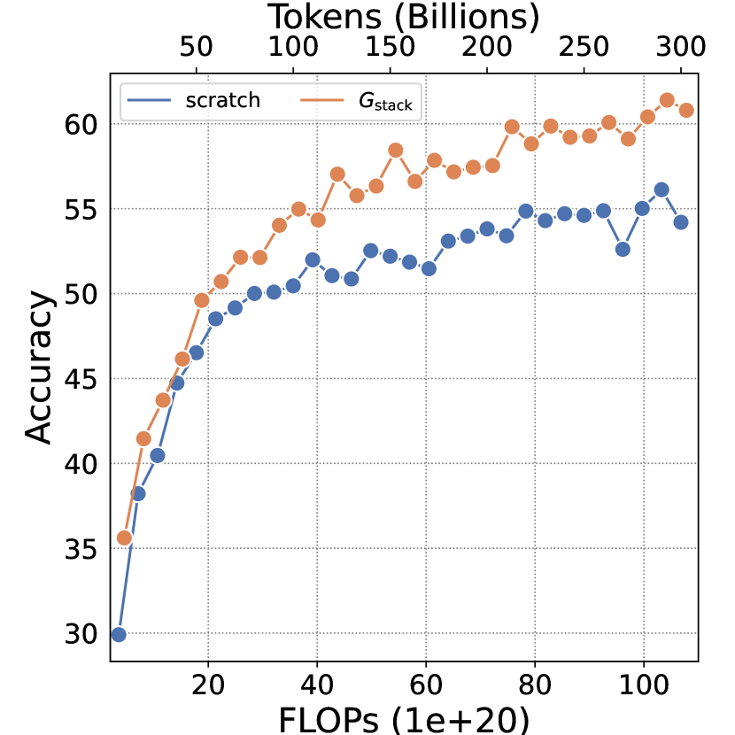
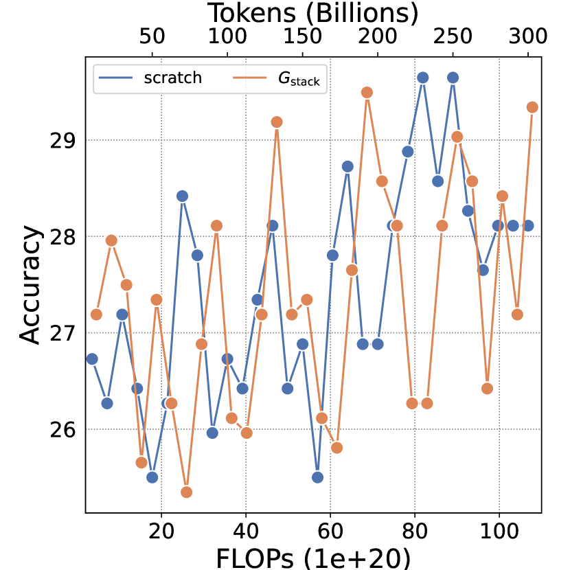
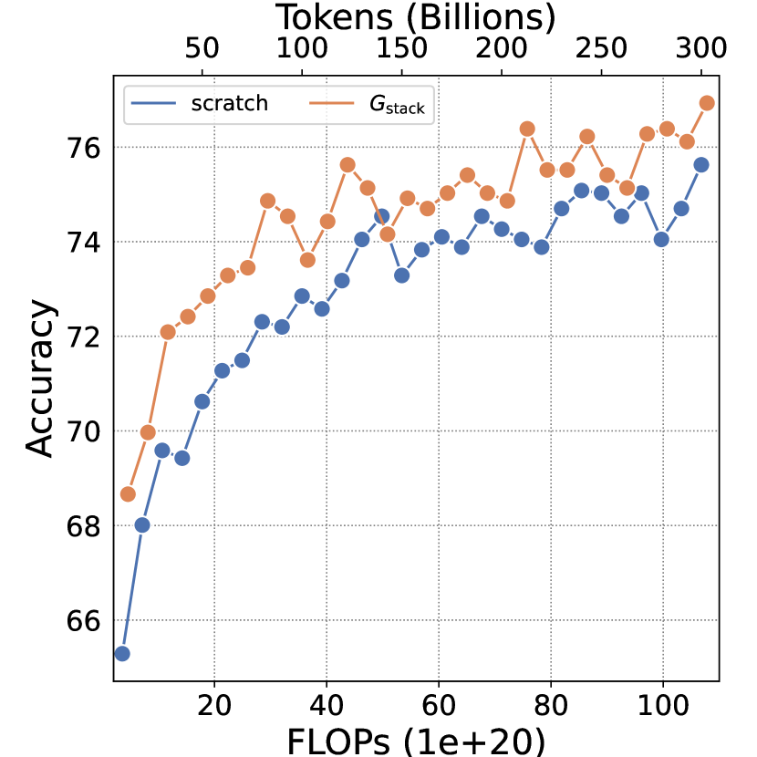
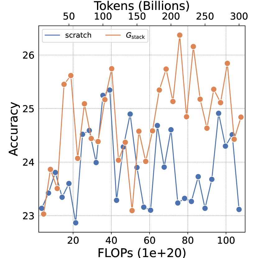
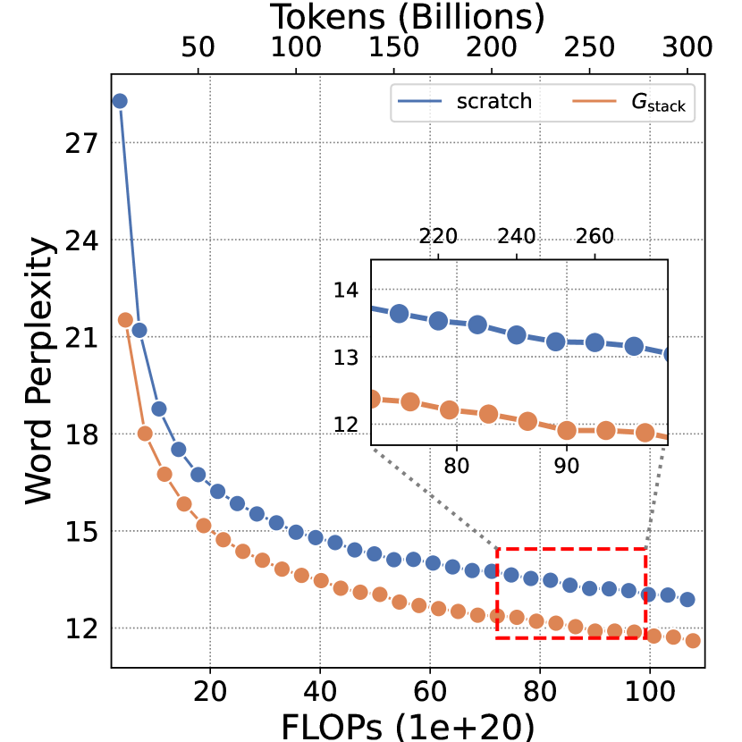
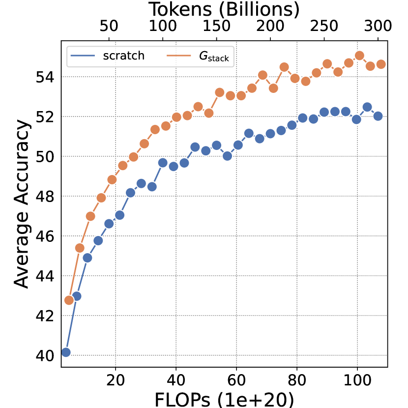
Our scaled-up experiments involve two larger model sizes: 3B and 7B. We initially train smaller models with a layer count that is one-quarter of our target layers (growth factor ), utilizing 10B tokens (). Then, we train the stacked models using over 300B tokens () for both sizes. Figures 4 and 5 show the loss, and the NLP benchmarks average accuracy evaluated using the Harness evaluator for training 3B and 7B LLMs with 300B tokens, respectively. 222In this study, we always calculate the consumption by combining the FLOPs required for both training small models and large models. So given , the consumption for training small model equals to the cost for training , so the plotted curves for actually starts at . The acceleration of is consistent across two models and all evaluation metrics. For instance, considering the 3B model, Figure 4 demonstrates that achieves a 54.5% speedup in pre-training, improvement of 2.1 in NLP benchmarks average accuracy compared to the baseline 3B model trained with 240B tokens.
When comparing the 1B, 3B, and 7B models, it is evident that the benefits of are not reduced as the model size increases, implying that its acceleration effect can be leveraged even with larger models. Details of the evaluation results, including evaluation with instruction tuning, can be found in Appendix D. Appendix E compares our baselines with the open-source LLMs Pythia and tinyLlama.
Scaling Training Tokens for .

We next evaluate the scalability of the stacking operator on another dimension - training with more tokens. This is especially important in light of recent discussions about the validity of efficient training algorithms, which have sparked debate [21] over whether certain strategies may initially learn faster but ultimately perform similarly or worse than vanilla training methods when given more training data. Hence, we aim to pre-train a LLM using on a substantial amount of training tokens.
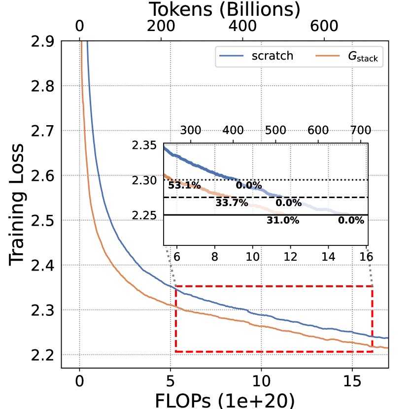
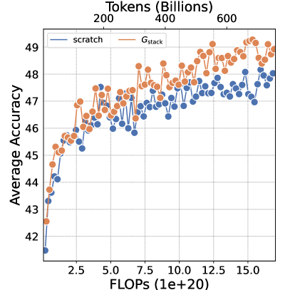
Concretely, we conduct an experiment on a 410M LLM using 750B tokens. Following the experimental setup in the previous section, we set growth ratio and growth timing and conduct continuous pre-training on the target 410M LLMs for 750B tokens. Compared to the chinchilla-recommended 8B tokens [4] for the 410M model, our experimental setting also surpasses this value by nearly 100 times, reaching 750B tokens.
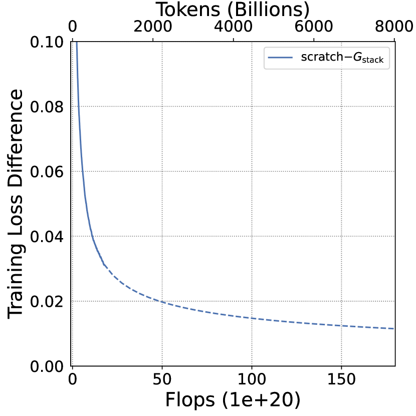
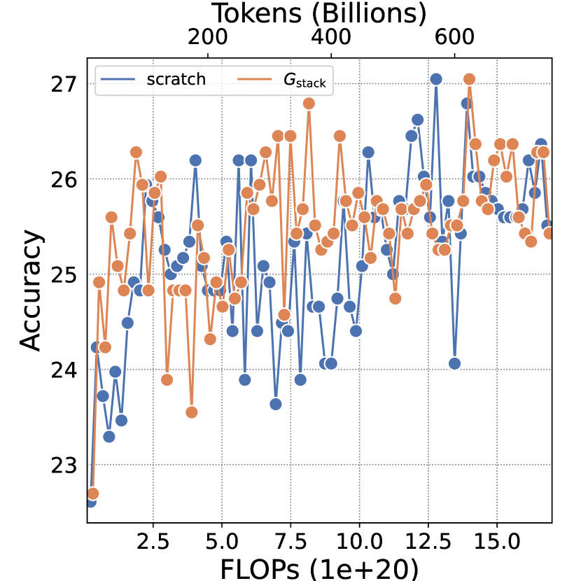
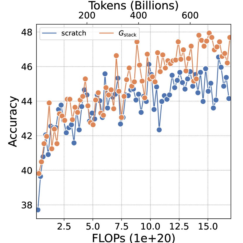
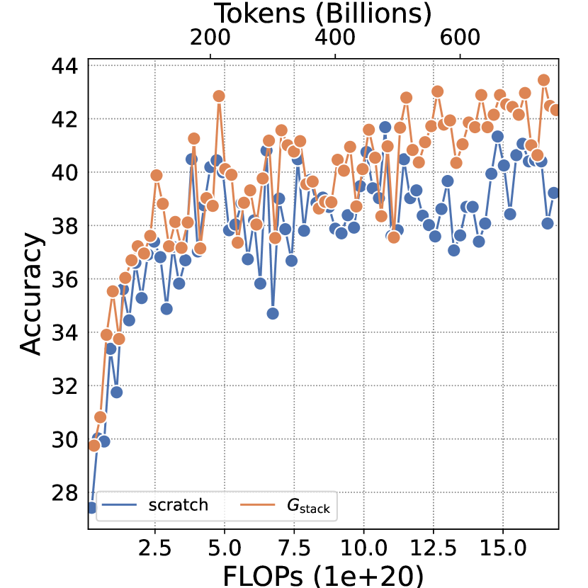
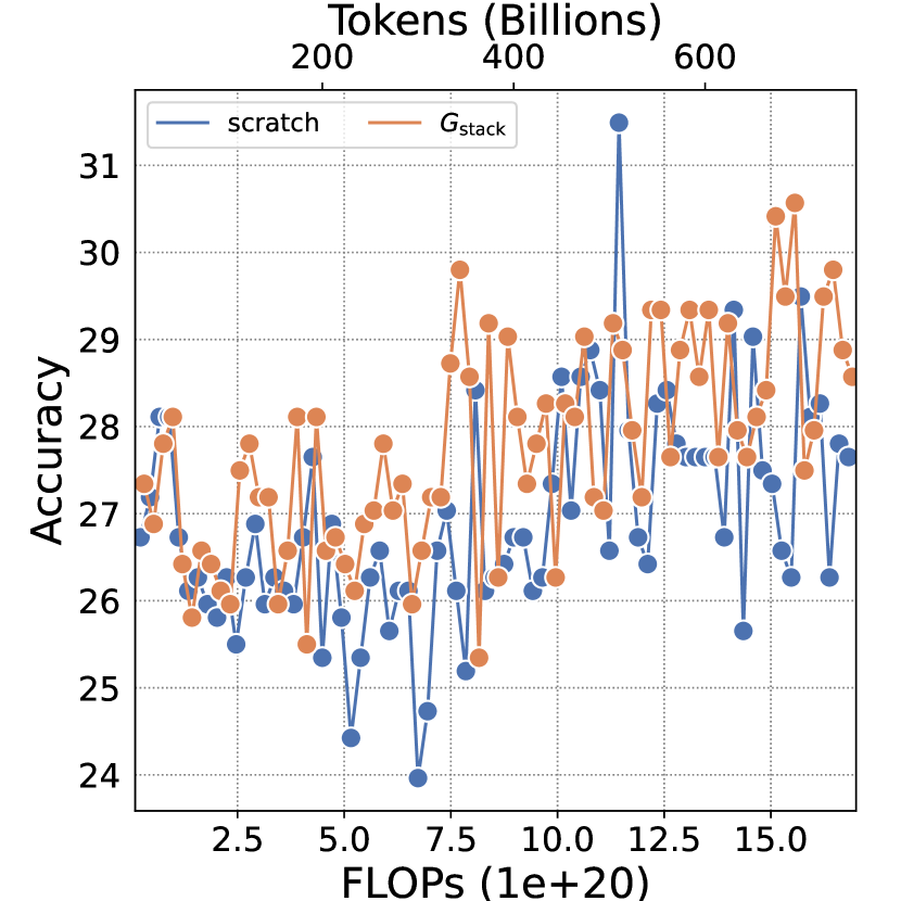
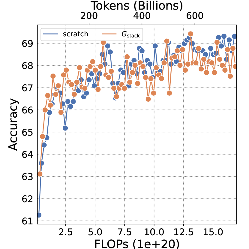
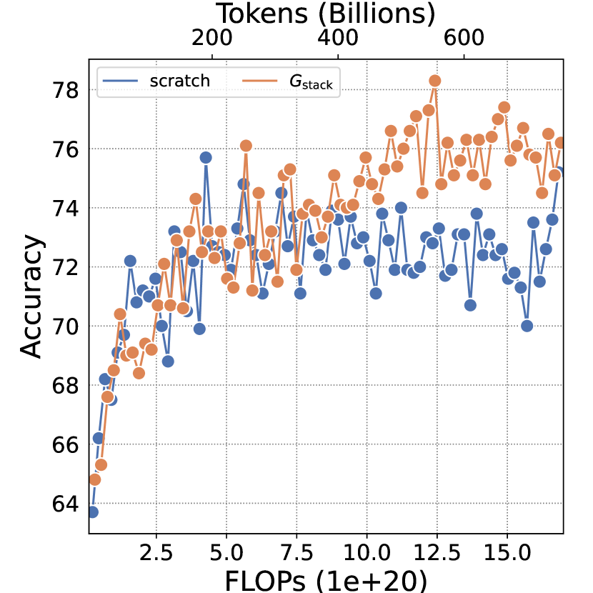
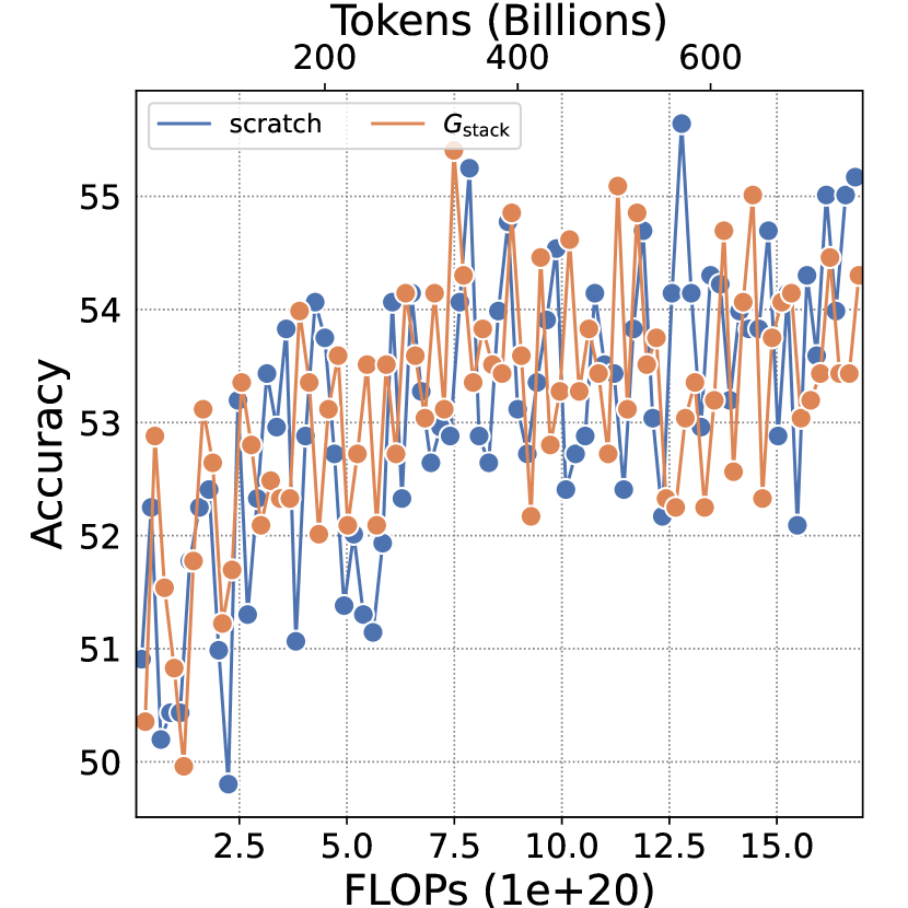
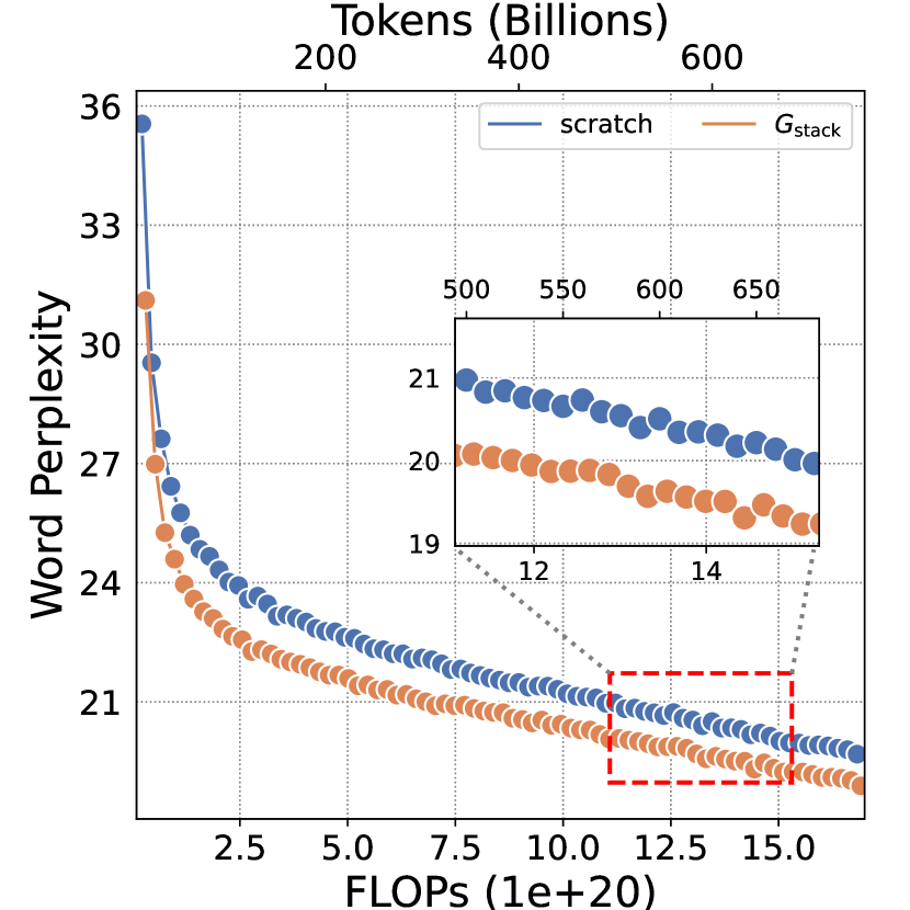
The training dynamics on Figure 6(a) indicate that remains effective in such cases. Details of the evaluation results with the similar findings can be found in Appendix D.3. Building upon the exceptional stability of LLM pre-training [37, 38], we estimate loss improvements and plot them in Figure 6(b). The fitting curve indicates will continue to exhibit acceleration effects even after 8T tokens, which is over 1000 times longer than the recommended token number [4]. It is also notable that this loss improvement after 8T training is not trivial for LLM pre-training, as previous studies [39] suggest that even minor improvements in the later phase can have a relatively substantial impact on downstream performance.
From a LLM practitioner’s perspective, this is also crucial considering “overtraining”, which involves training LLMs with significantly larger amounts of data than recommended by scaling laws [3, 4, 5], a common practice that has become prevalent. A notable example is the training of LLama 3-8B with 15T tokens, which is nearly 100 times greater than the token count recommended by the chinchilla scaling laws [4]. Hence, this finding provides confidence in the consistent excellent acceleration of throughout the entire practical LLM pre-training process.
Estimating Scaling Laws.
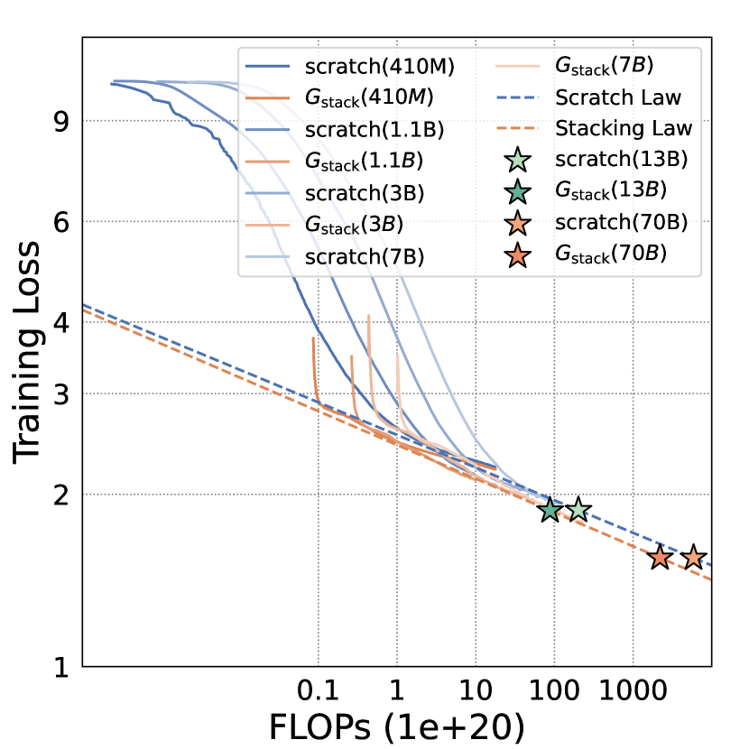
To further explore our findings, we graph our four models (410M, 1.1B, 3B, and 7B) on the same figure and attempt to uncover our “scaling law” using the operator. Following [3, 4], we define the scaling power law using the equation , where and are constants we need to fit, represents the FLOPs, and denotes the model’s final loss under this FLOP. We use the curve_filt function in SciPy [40] to fit both the scratch model and the model and present the estimation scaling law in Figure 7. The figure shows that our scaling law exhibits improved efficiency compared to the scaling law estimated from baseline LLMs, achieving the same target loss while requiring much less computational resources. However, in light of the significant computational resources devoted to other scaling law studies [3, 4], we acknowledge that our scaling law is an initial estimate subject to computation constraints, and a comprehensive study is left for future research.
4.2 Determining Growth Timing and Growth Factor for Using
We comprehensively validate the effectiveness of the compared to training from scratch in Section 4.1. However, to incorporate into a LLM’s pre-training process, we need to determine two crucial hyperparameters: the growing time () and the growing factor (). In our previous experiments, we rely on ad-hoc choices for these parameters, thereby lacking a systematic approach to determining them when use . There exists research on investigating the growth timing [41], but the settings are quite different from the LLM pre-training. Therefore, this section offers a clear guide for practitioners looking to optimize using the operator in LLM pre-training processes.
We begin by offering a formal definition. When given a computational budget , established scaling power laws [3, 4] exist to guide the non-embedding parameters and the number of training tokens to achieve the lowest model loss in the case of training from scratch. However, tuning hyperparameters becomes more complex when the fixed budget is allocated to find the optimal model training strategy using the operator, which involves two training phases. Consequently, the overall computational budget can be expressed as the sum of the two components: . Here, and represent the flops required to train the initial small models , and the large model respectively, where and denote the parameters and training tokens of the small model, and and represent the parameters and training tokens of the large model. Since the large model is grown by a factor of such that , we have .
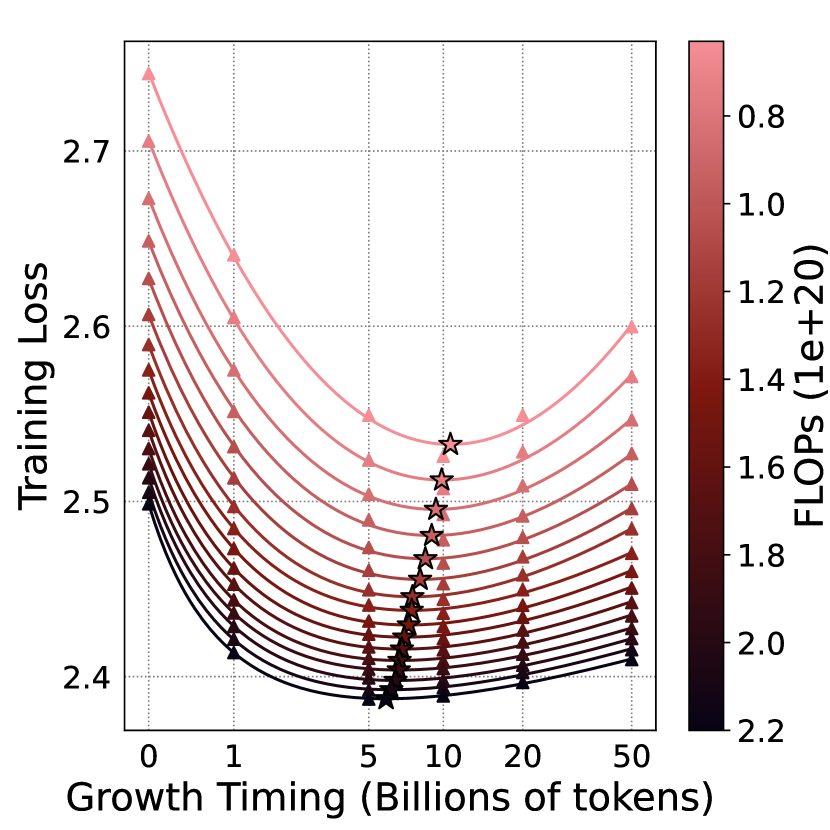
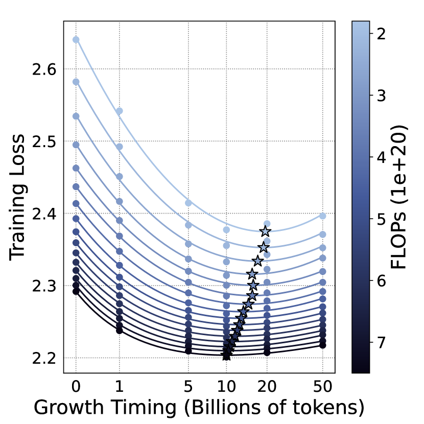
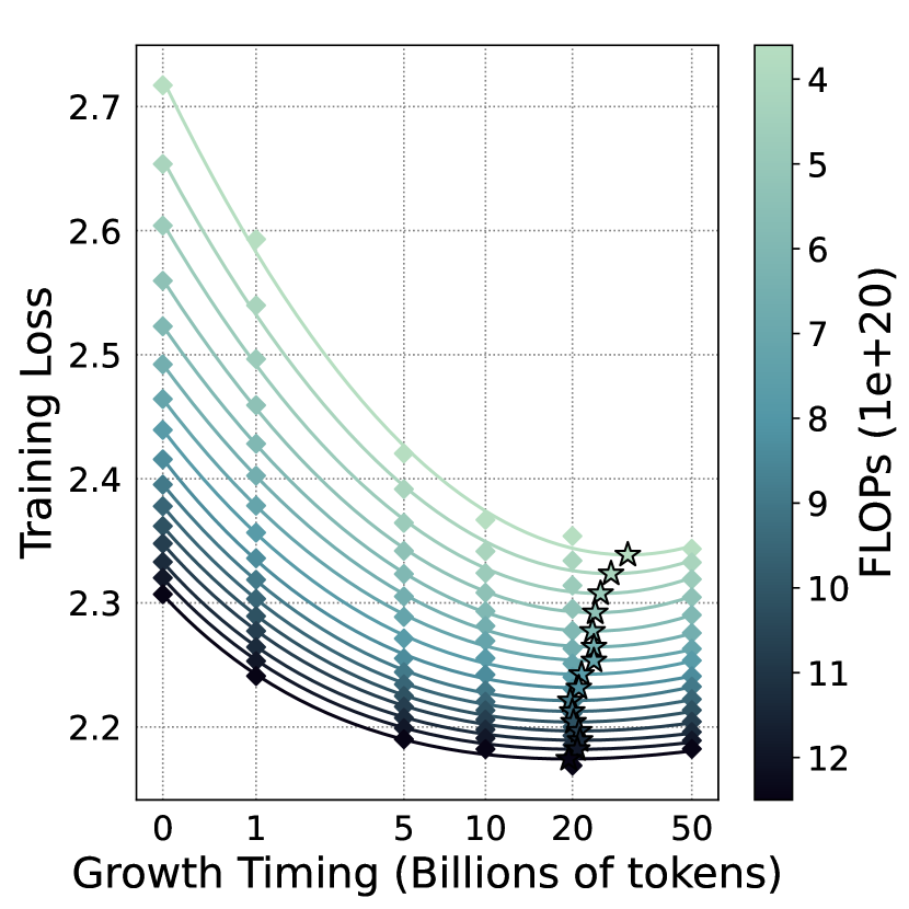
So when given a budget , our objective is to identify the optimized values , , , that minimize the loss . However, simultaneously optimizing the above four variables can be computationally expensive. Therefore, instead of searching for global optimals, we separately determine two factors closely related to the : the training tokens for the small model (growth timing) and the growth factor :
| (1) |
Determining Growth Timing: .
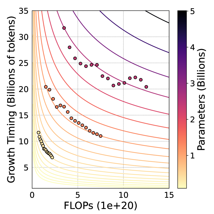
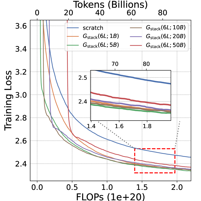
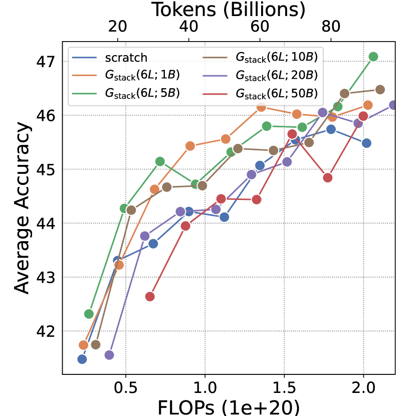
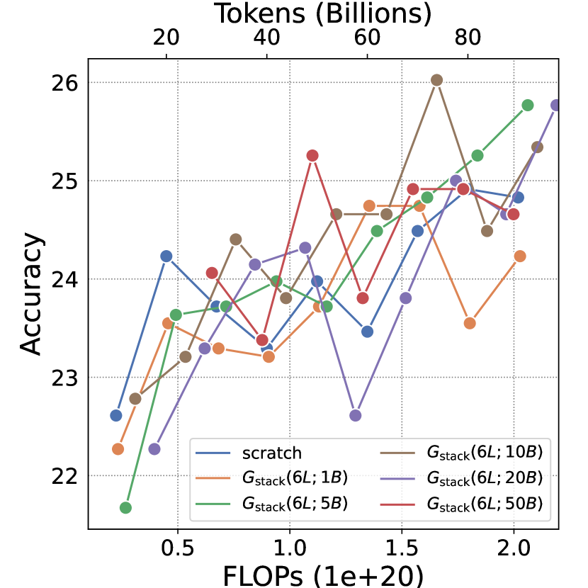
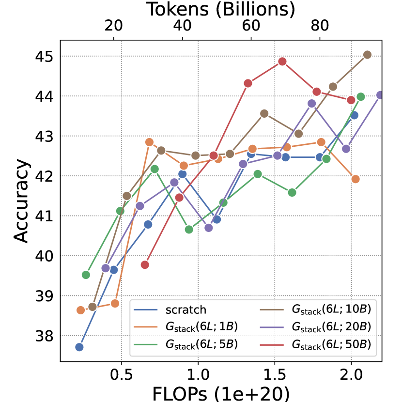
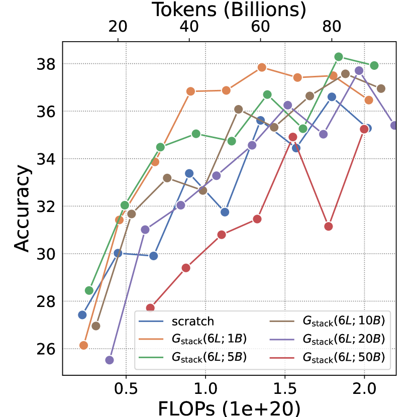
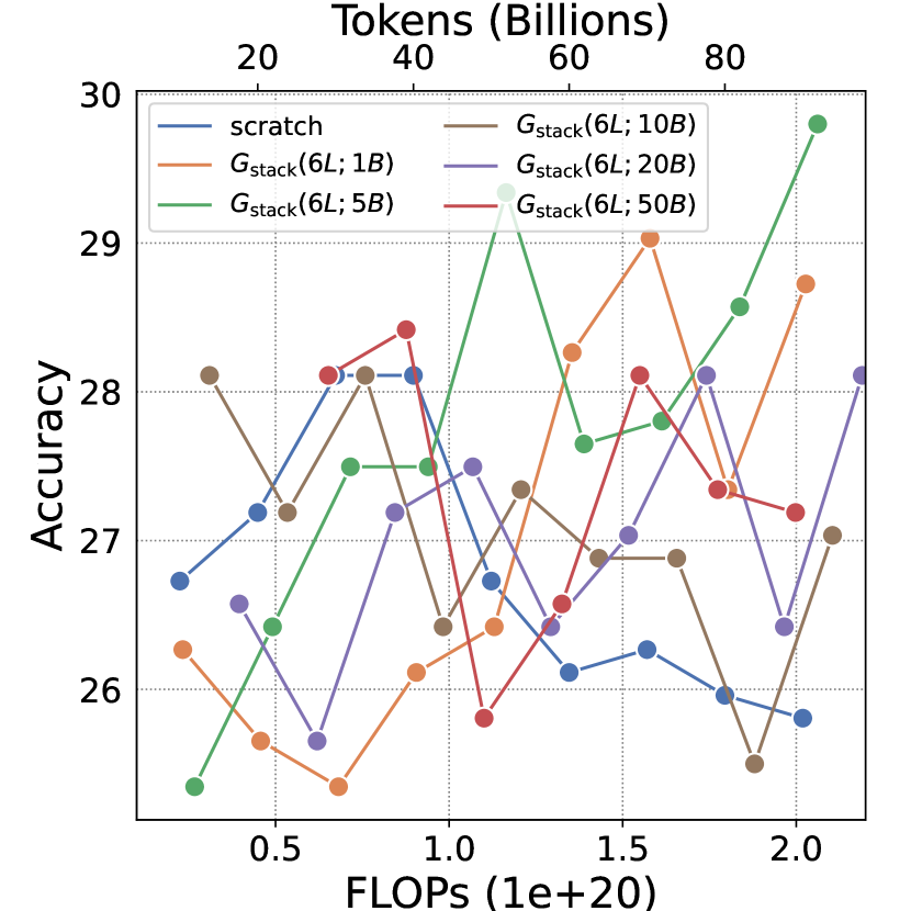
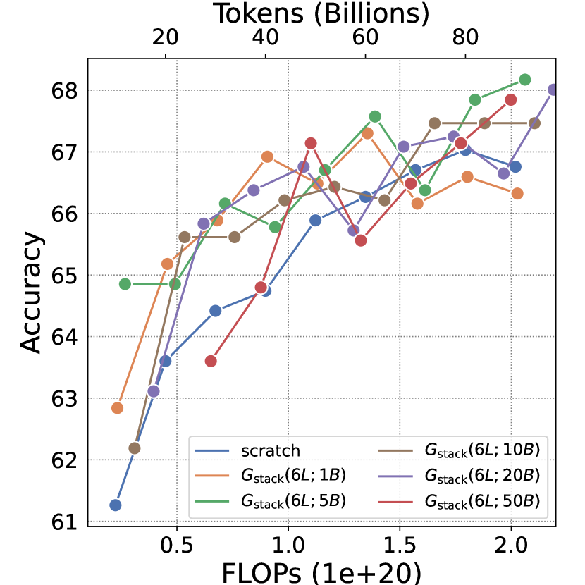
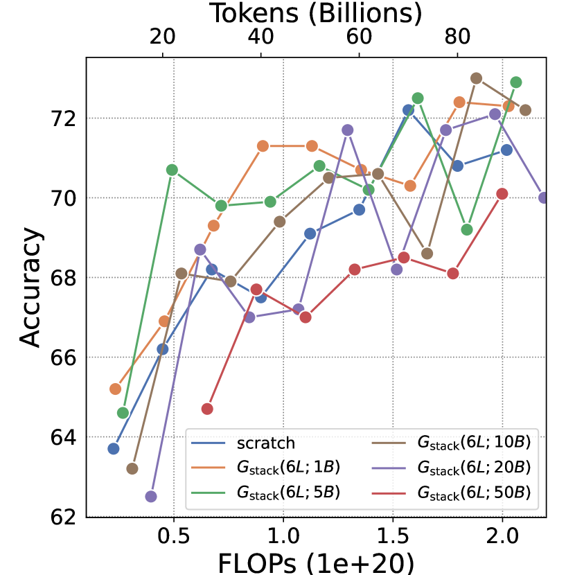
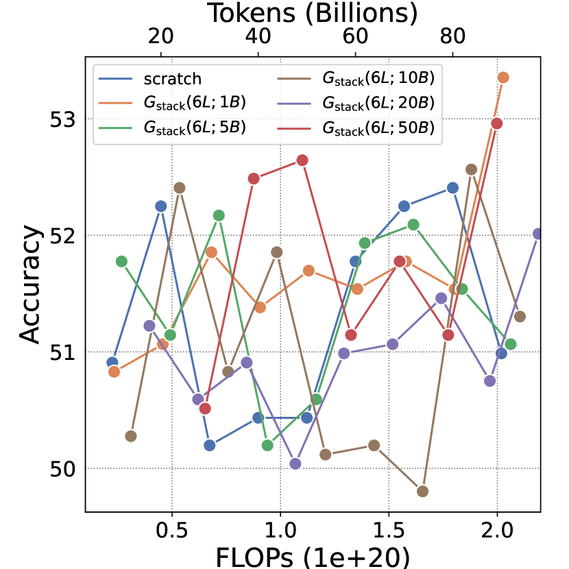
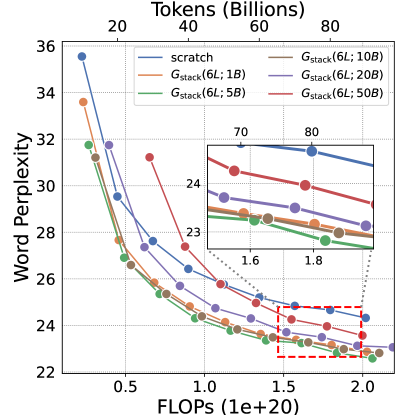
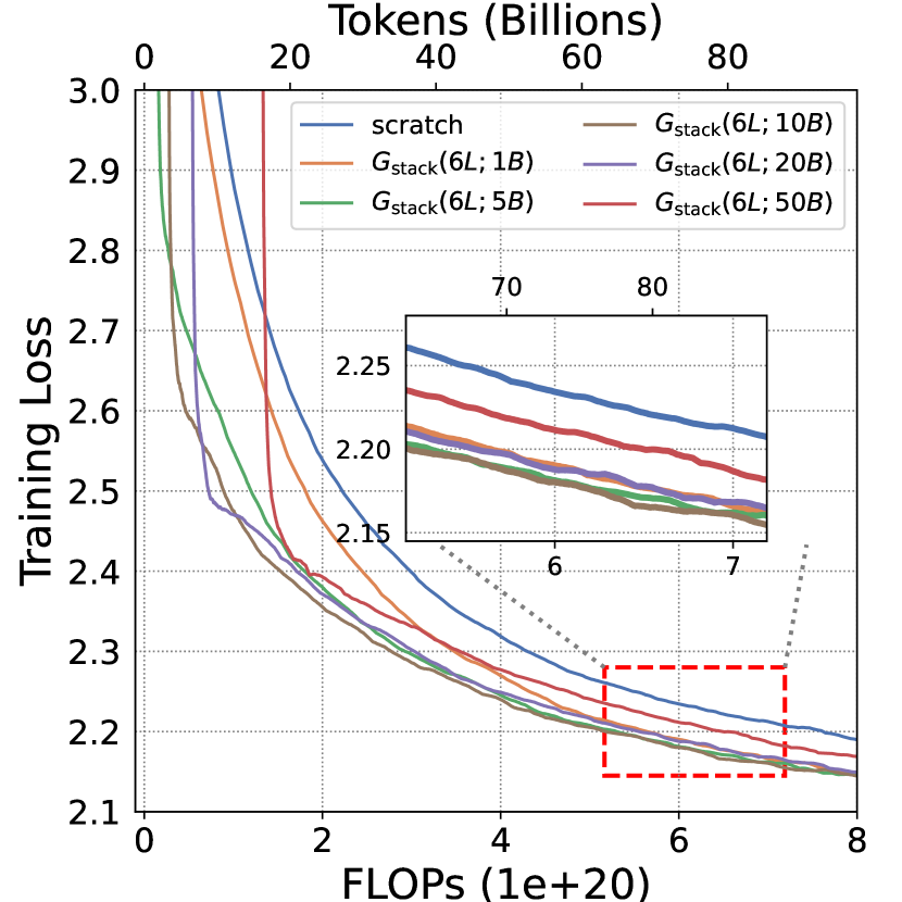
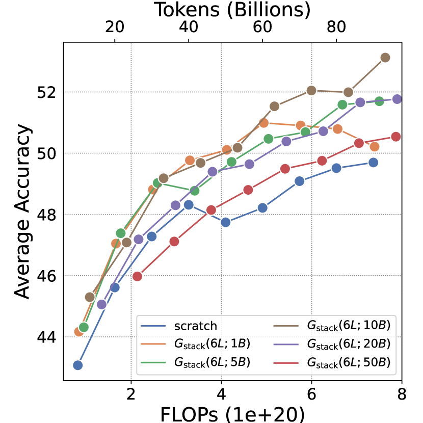
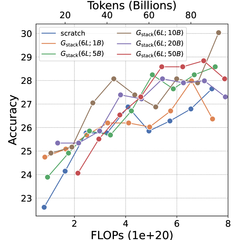
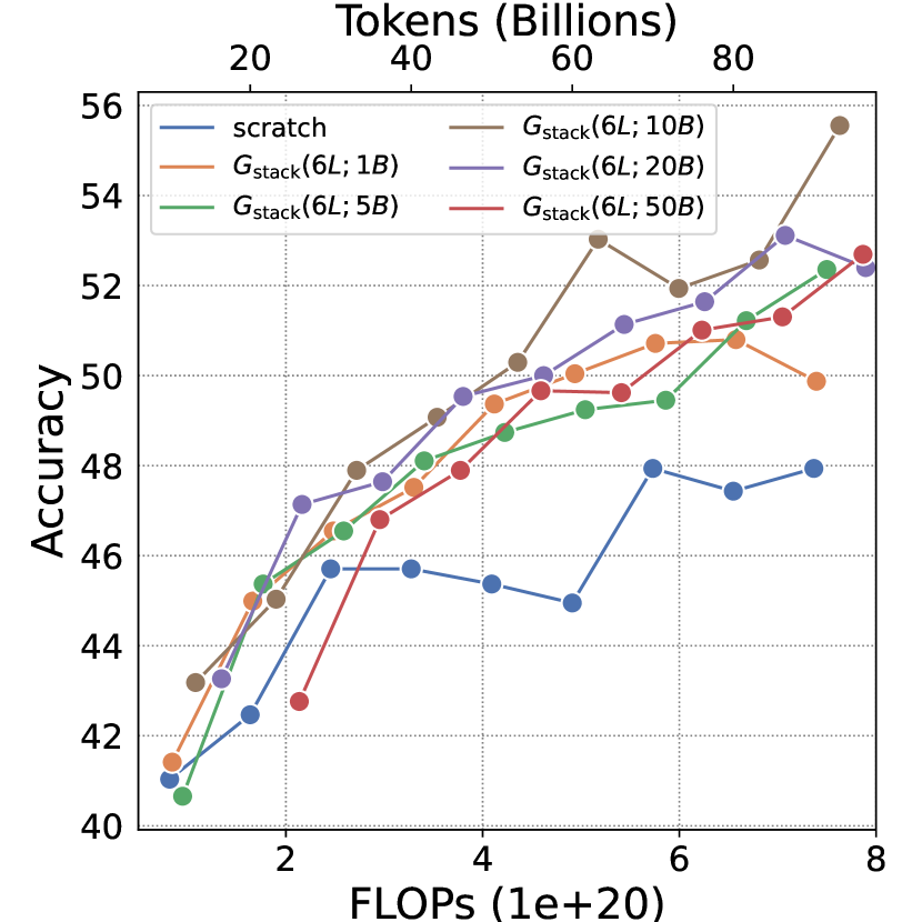
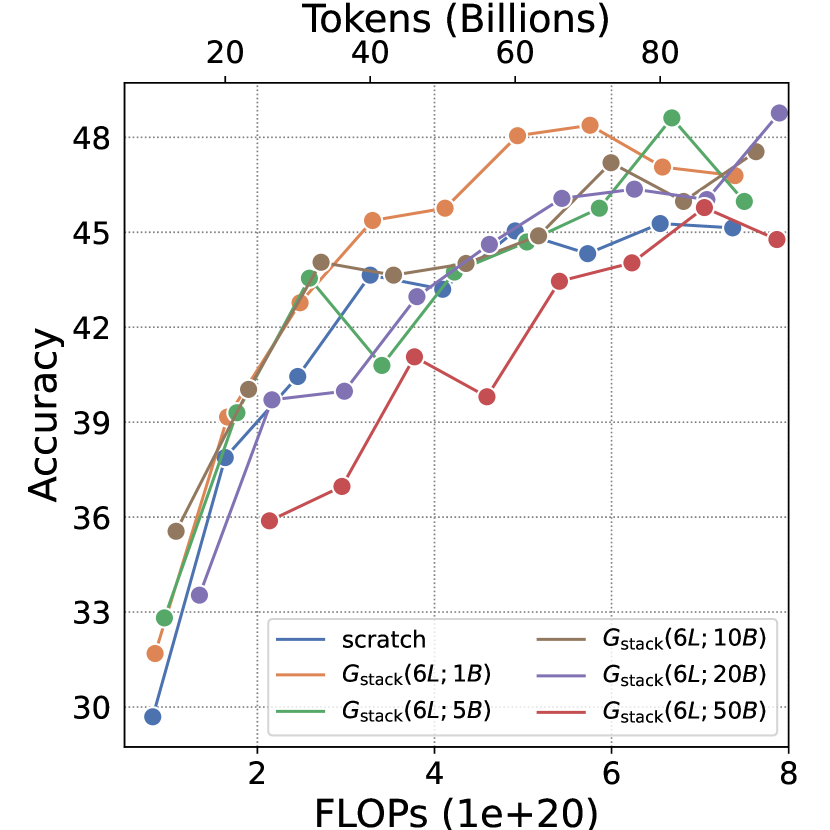
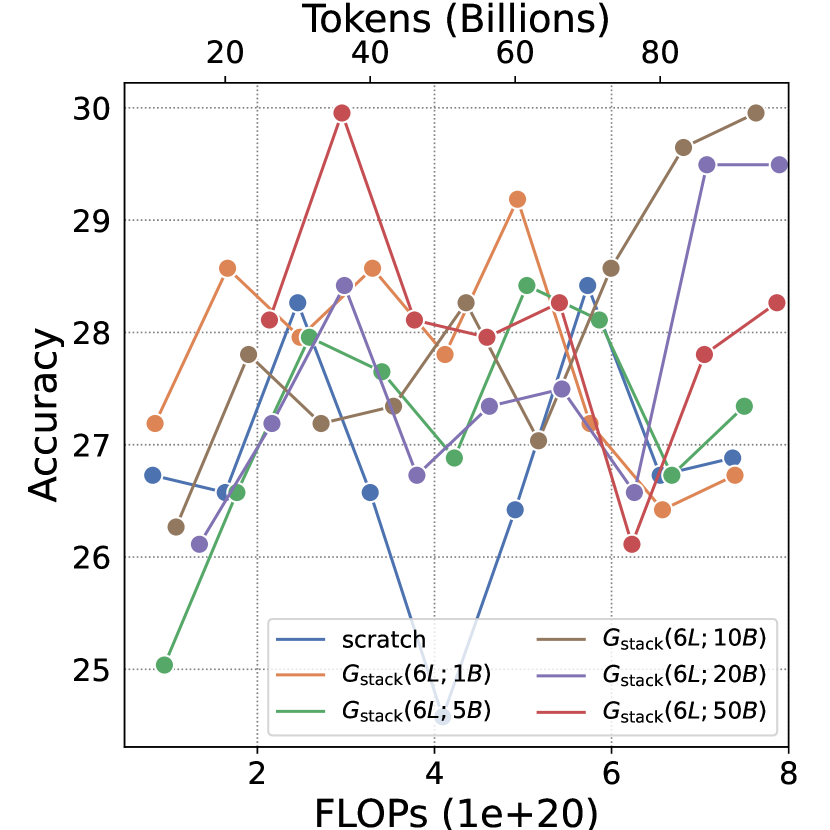
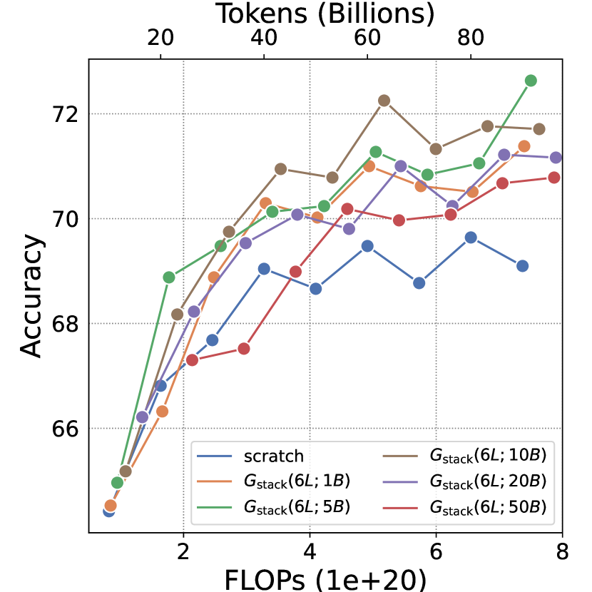
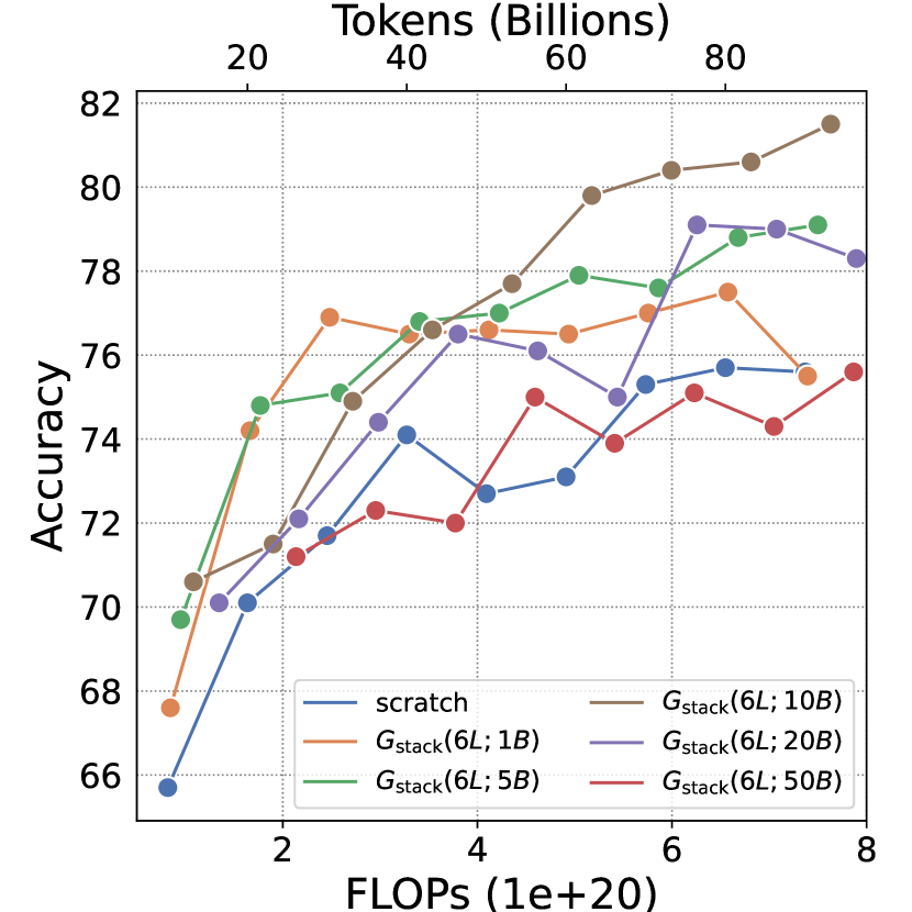
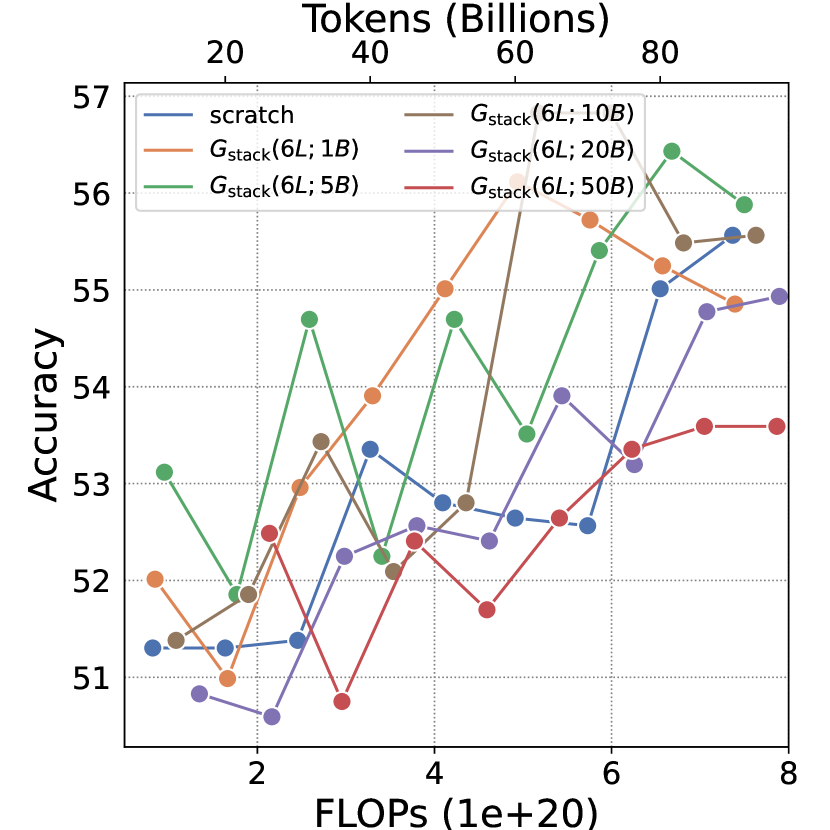
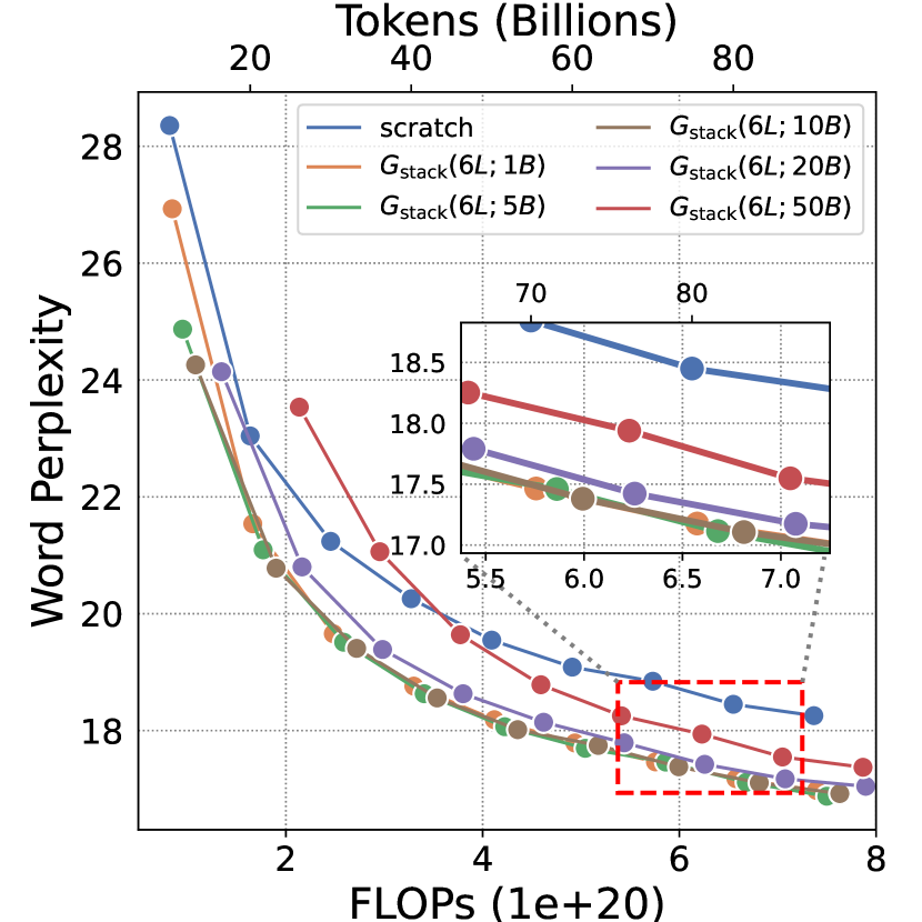
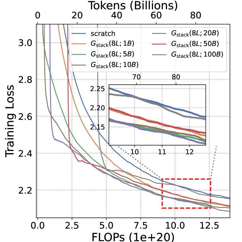
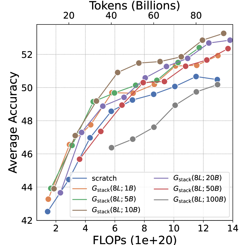
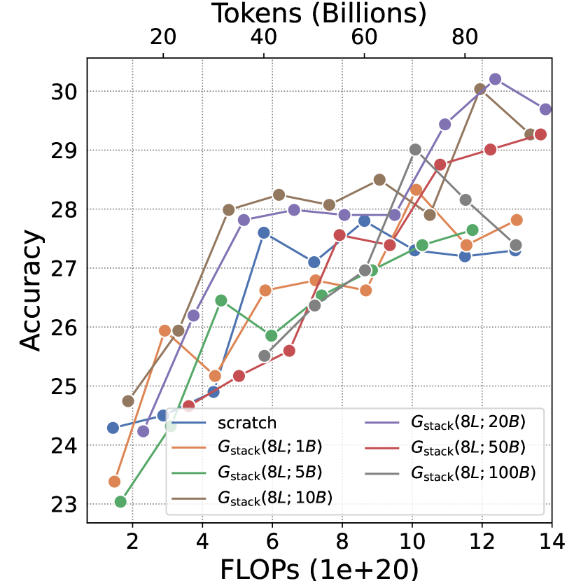
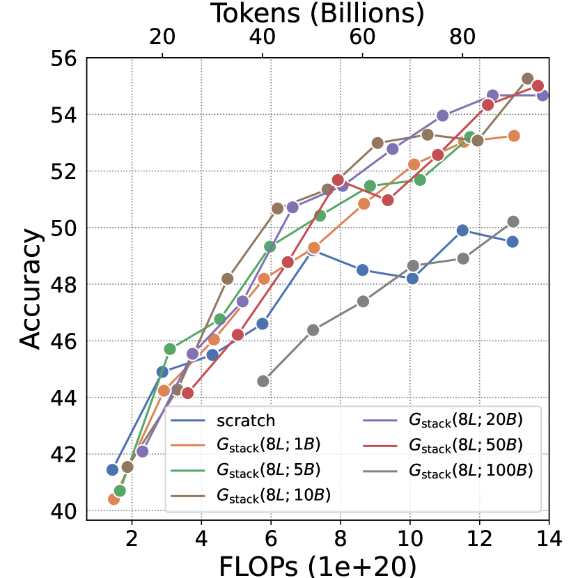
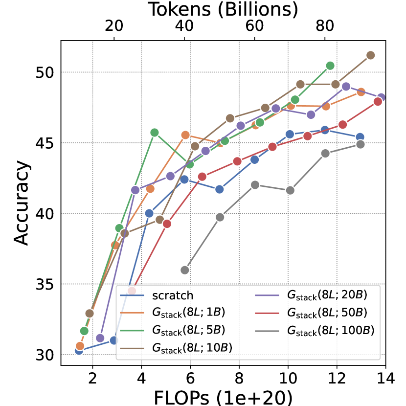
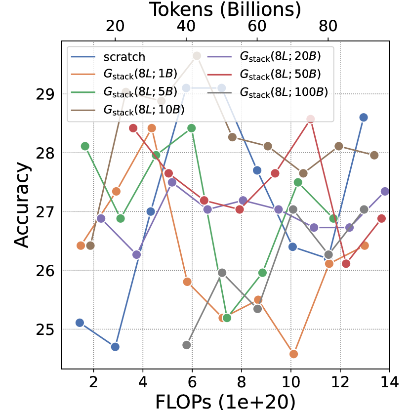
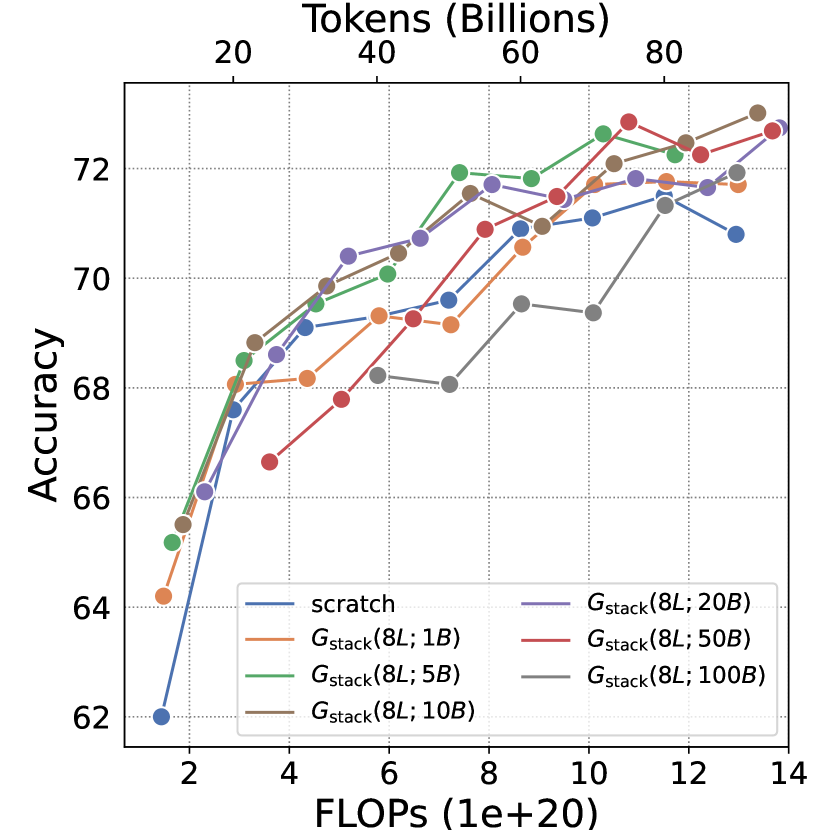
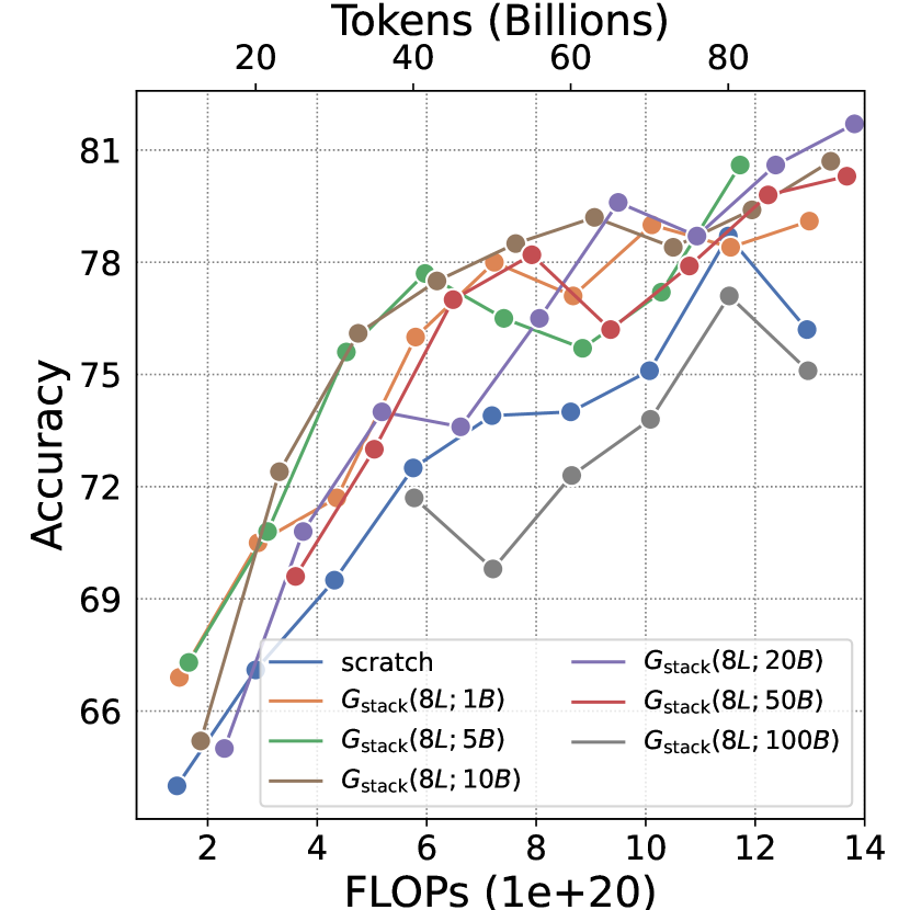
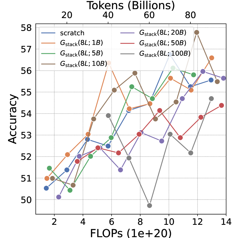
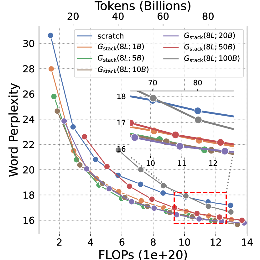
We first explore the effect of growth timing, i.e. the training token for the small model. Particularly, we apply the operator to a series of small models trained with tokens. Subsequently, we stack them to the target layers with growth factor and train for a fixed set of computational FLOPs. We replicate the above experiments using three target model sizes and plot each set of IsoFLOP points in Figure 8(a), 8(b) and 8(c). Surprisingly, even a small model trained with just tokens exhibits a significant speedup compared to the directly stacking small random initialized models (represented as “0B”). While 0B’s performance is similar to models trained from scratch, implying stacking itself does not serve as an effective initialization method. Furthermore, by applying smoothing techniques to model IsoFLOP curves as parabolas, we identify the optimized value of that minimizes loss for each FLOP count, leading us to hypothesize the existence of a logarithmic equation involving , , and :
| (2) |
After fitting, we obtain , and and we plot the contour figure in Figure 9. It can be observed that our estimated curves align well with the actual optimal points.
Determining Growth Factor: .
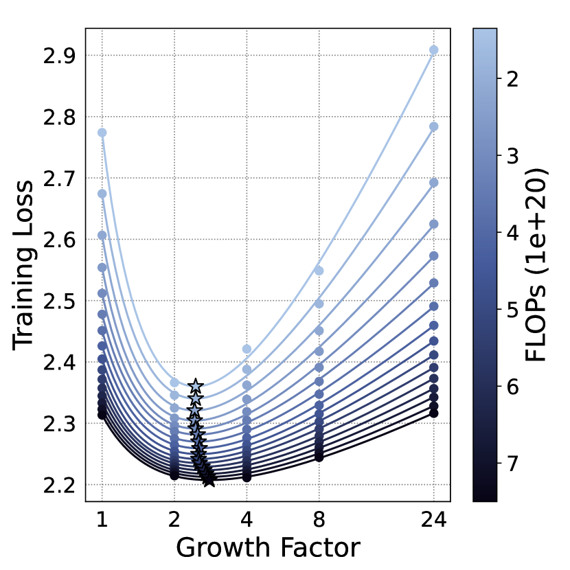
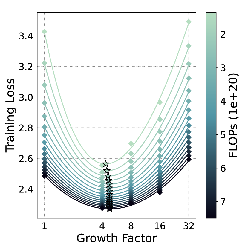
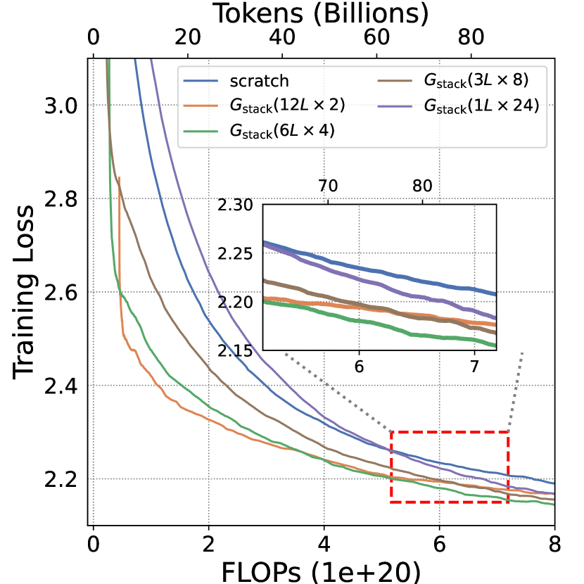
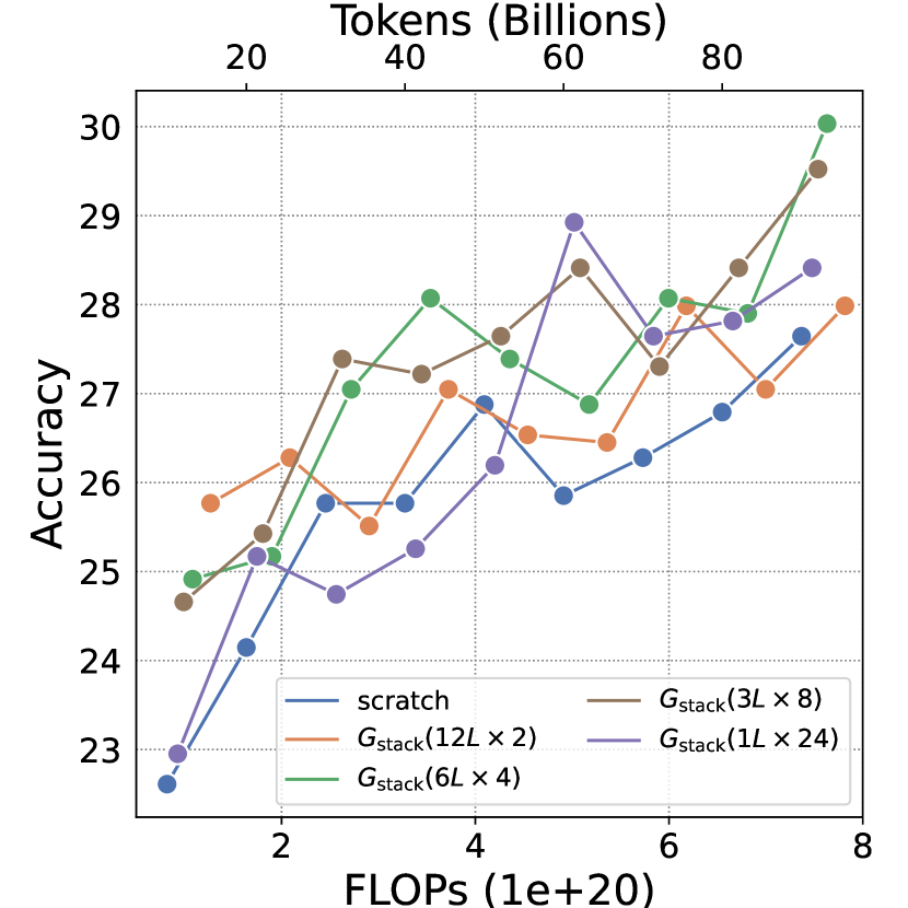
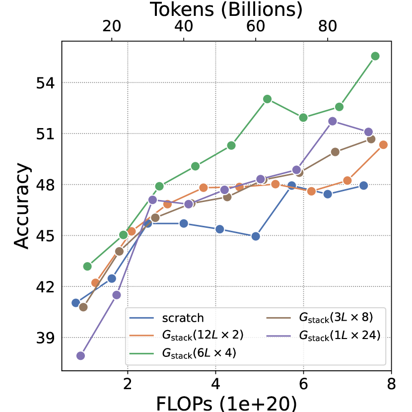
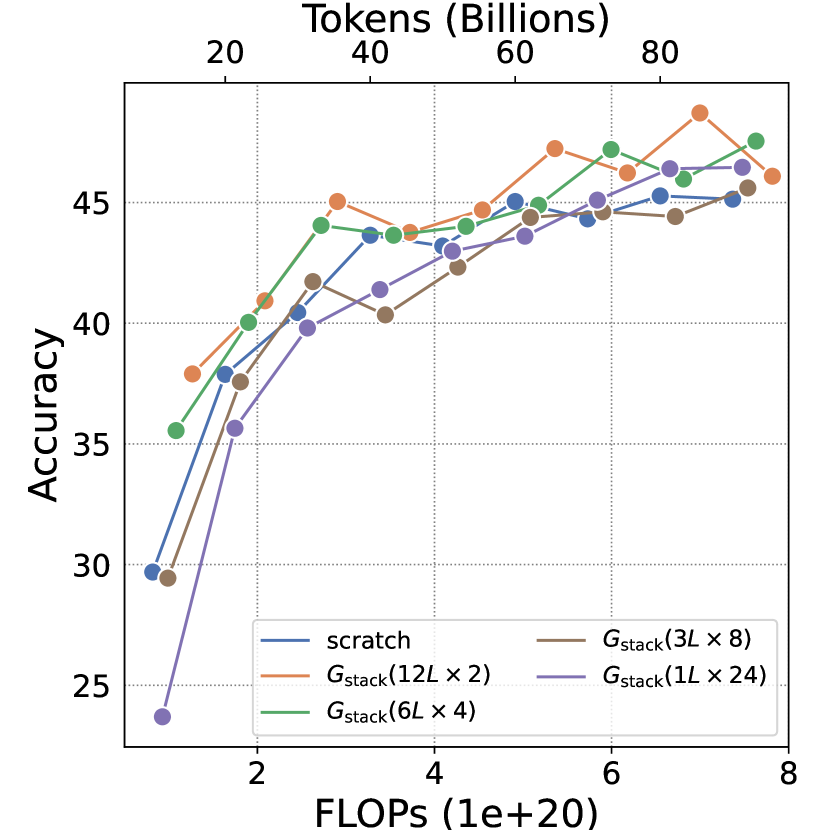
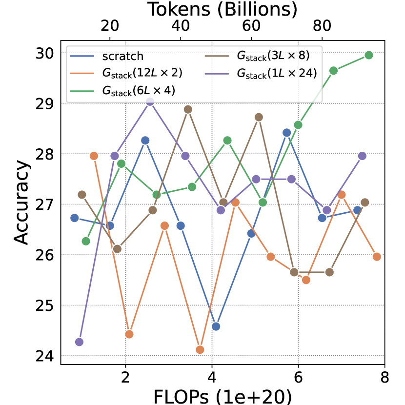
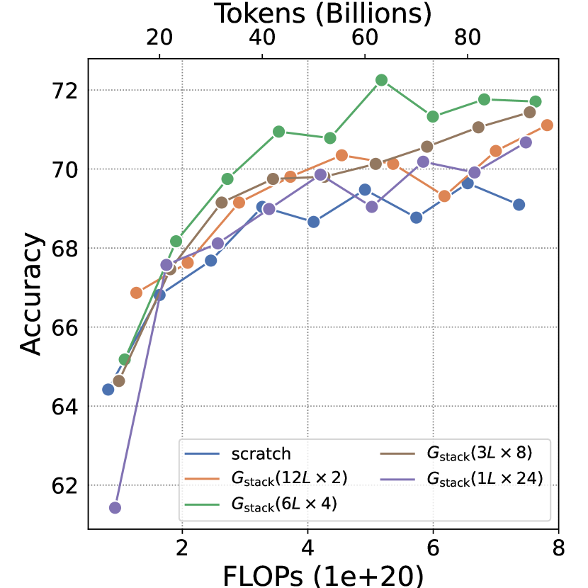
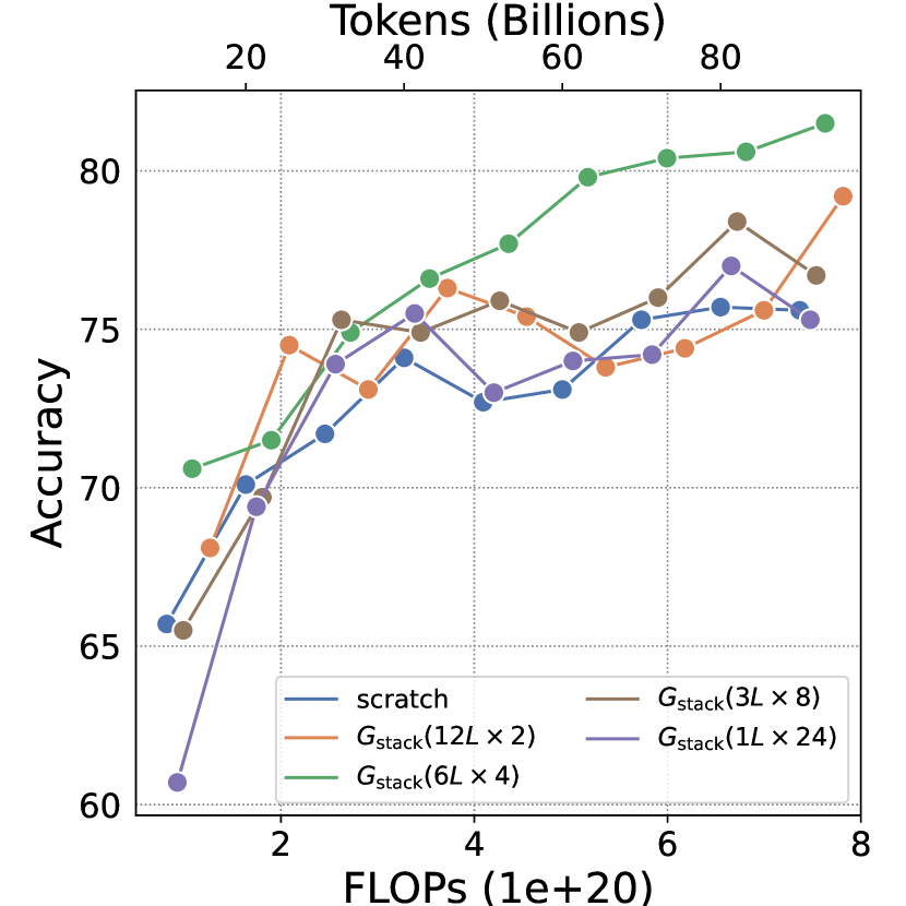
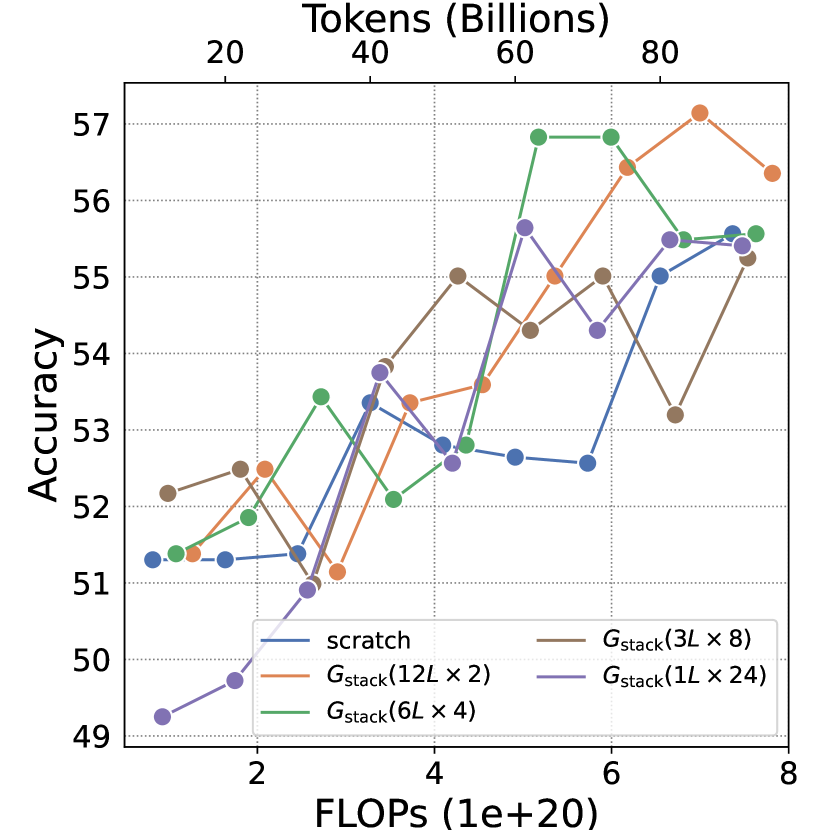
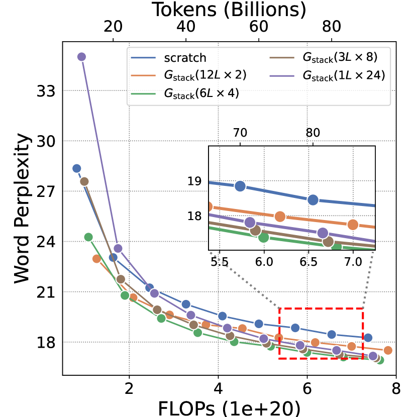
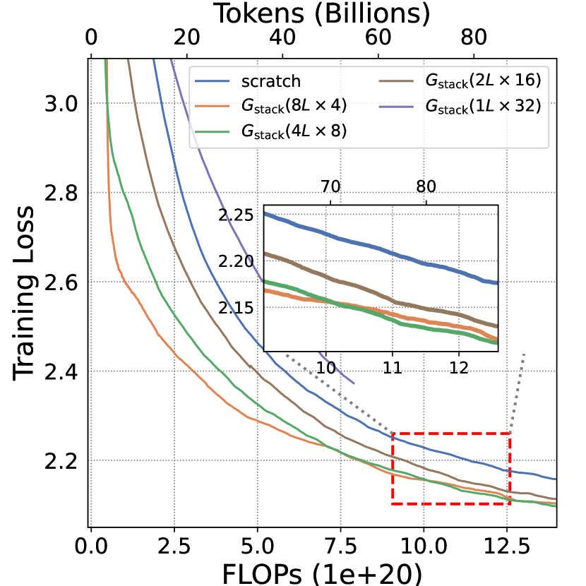
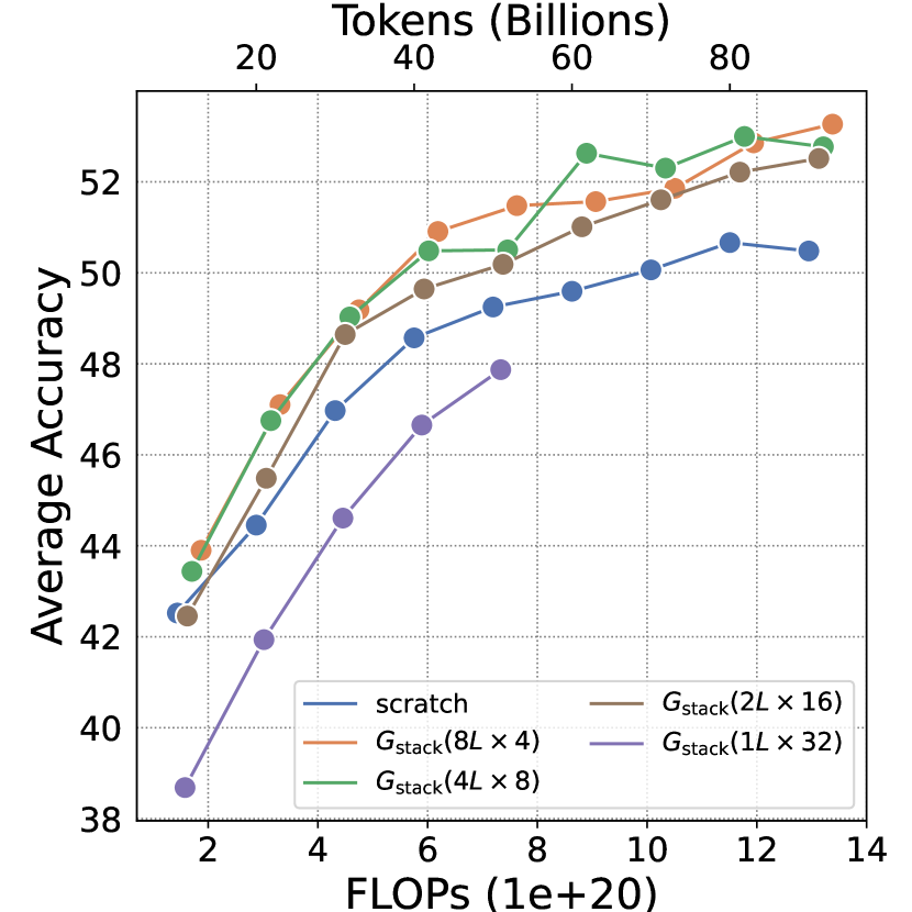
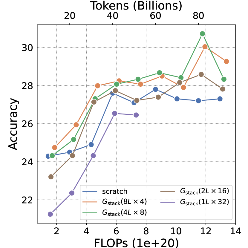
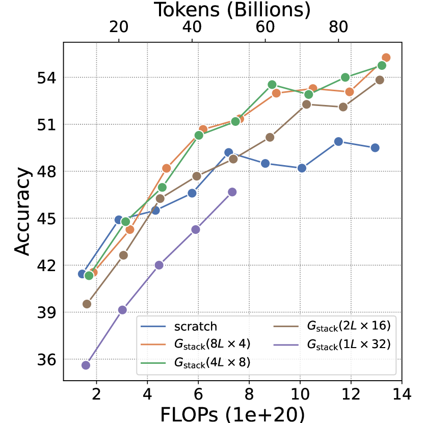
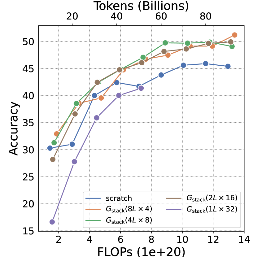
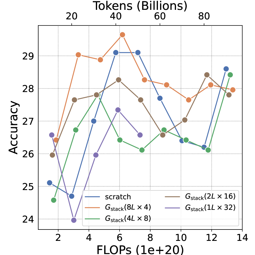
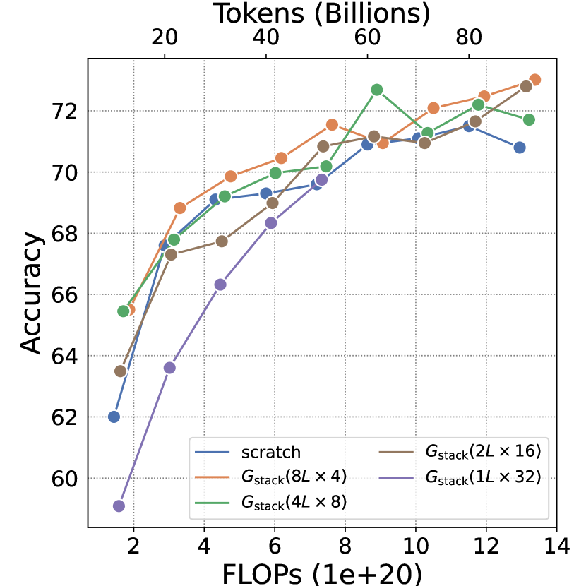
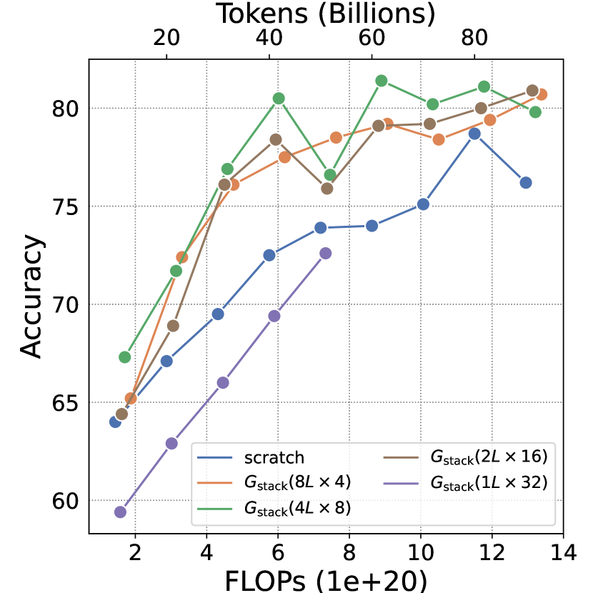
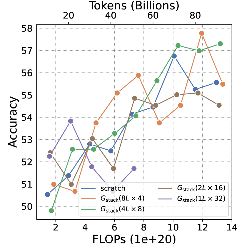
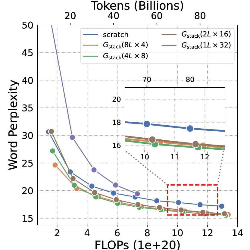
Another factor we determine is the growth factor . As models with 3B and 7B parameters have identical depths, we run experiments using two model sizes: 1.1B (24 layers) and 3B (32 layers). Specifically, we vary the stack factors to for the 1.1B model and for the 3B model while keeping the base models trained with B tokens. The smoothed IsoFLOP curves are plotted in Figure 10. Interestingly, even with a relatively shallow 2-layer base model and a growth factor of , we observe a remarkable improvement compared to the baseline 3B model (). However, when using a 1-layer base model, underperforms compared to the baseline. Our curves indicate that the optimal growth factor lies between 2 and 4.
However, unlike determining training token , we cannot generate sufficient data to estimate the relationship between , , and , due to computational constraints. Thus, this work suggests a constant growth factor of . We also include our preliminary estimated equation and contour figure for in the Appendix F. All evaluation results of Section 4.2 are listed in Appendix G.
5 Ablation and Discussion
To further give insights into adopting model growth techniques in LLM pre-training, we ablate variances for and discuss function preserving in general model growth techniques.
5.1 Ablation: How to Stack?
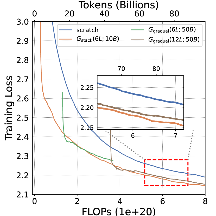
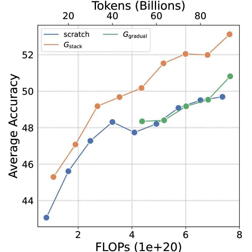
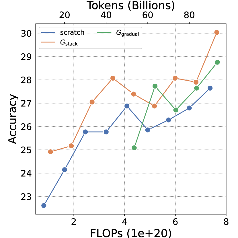
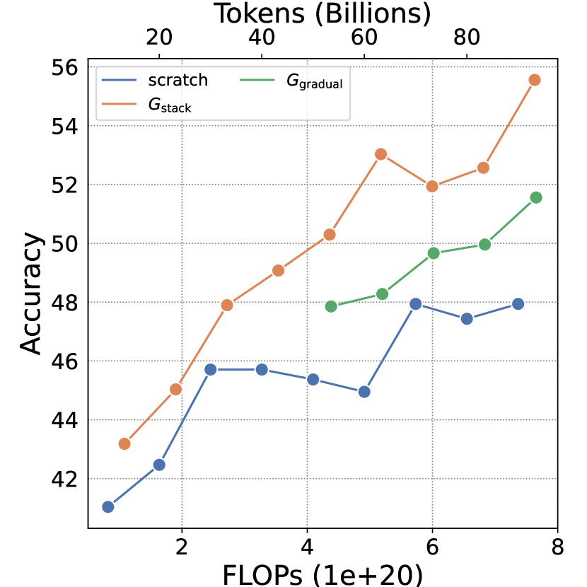
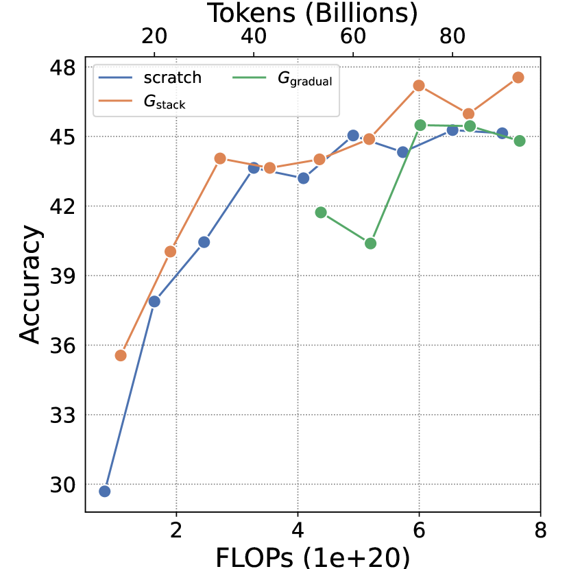
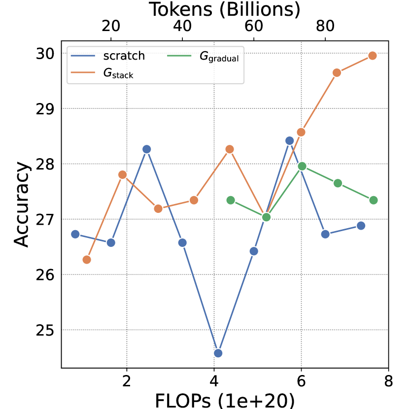
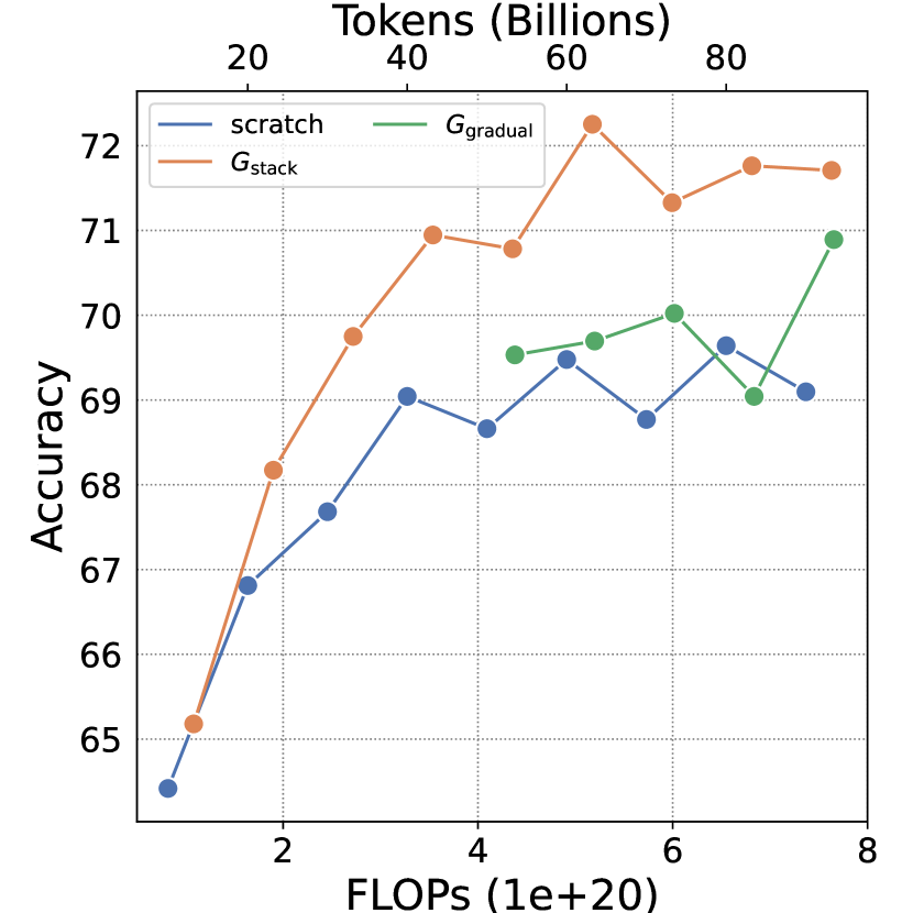
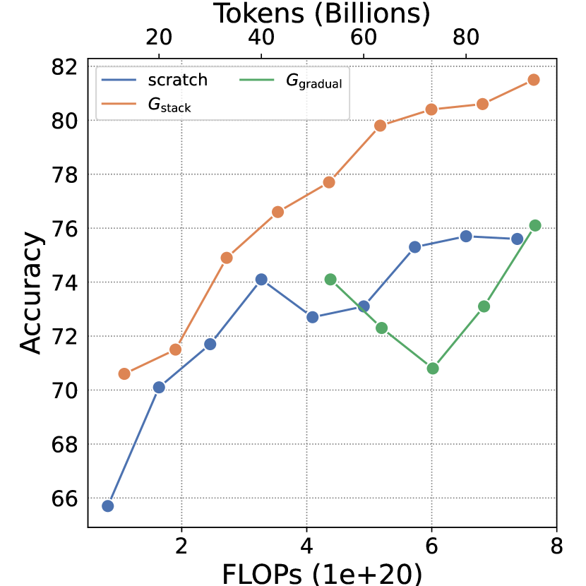
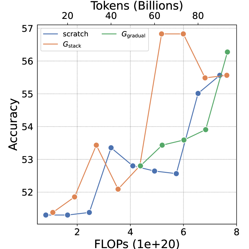
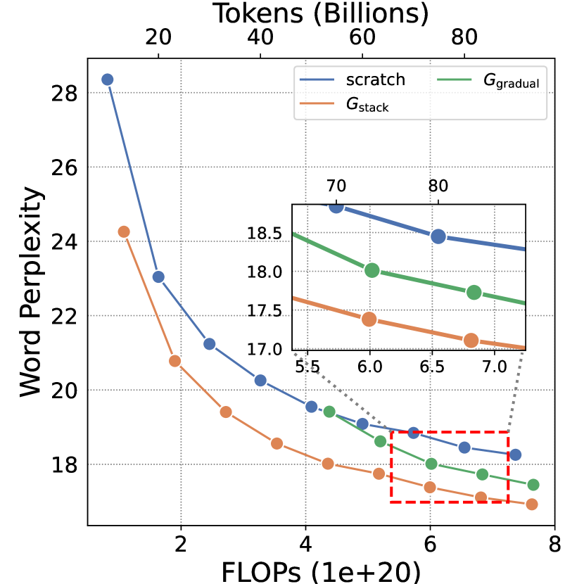
It is worth noting that differs from the algorithm proposed in StackedBERT [11], which utilizes a gradually stacking strategy. Hence, we compare our “one-hop” and their gradual stacking approach. Following the methodology introduced in StackBERT, we employ a two-step stack strategy. Given our target model size of 1.1B with 24 layers, we start with a 6-layer model. Subsequently, we train it on 10B tokens and double the model’s depth through stacking, repeating this step twice (train-stack-train-stack) to achieve the desired scale. Our experiments demonstrate that outperforms gradual stacking approaches on loss and downstream evaluations. For example, the evaluation results show that achieves a 2.4 higher average accuracy and 0.6 better Wikitext PPL than gradual stacking when pre-training large models for 100B tokens. The results can be found in Appendix H.1. We further compare other stacking variations, such as stacking via interpolation and partial stacking of certain layers which are also adopted in LlamaPro [42] and Solar [42, 43], and leave our detailed findings in the Appendix H.2 and H.3.
5.2 Discussion: Why Does Function Preserving Fail?
Function preservation (FP) is a key concept that underlies most model growth approaches [26, 10, 14, 19]. The idea is intuitive that a larger model should initialize parameters that can represent the same function as the ones in the smaller model, i.e. , where is the input. We give a mathematical definition of FP in the Appendix I.1.
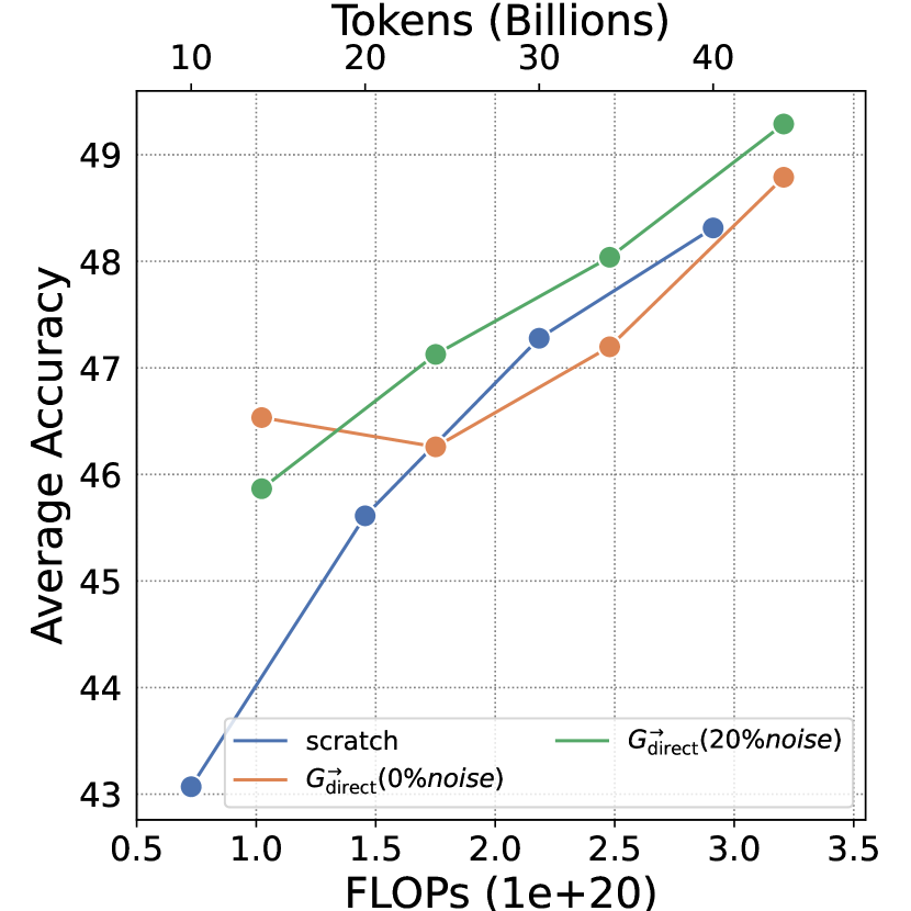
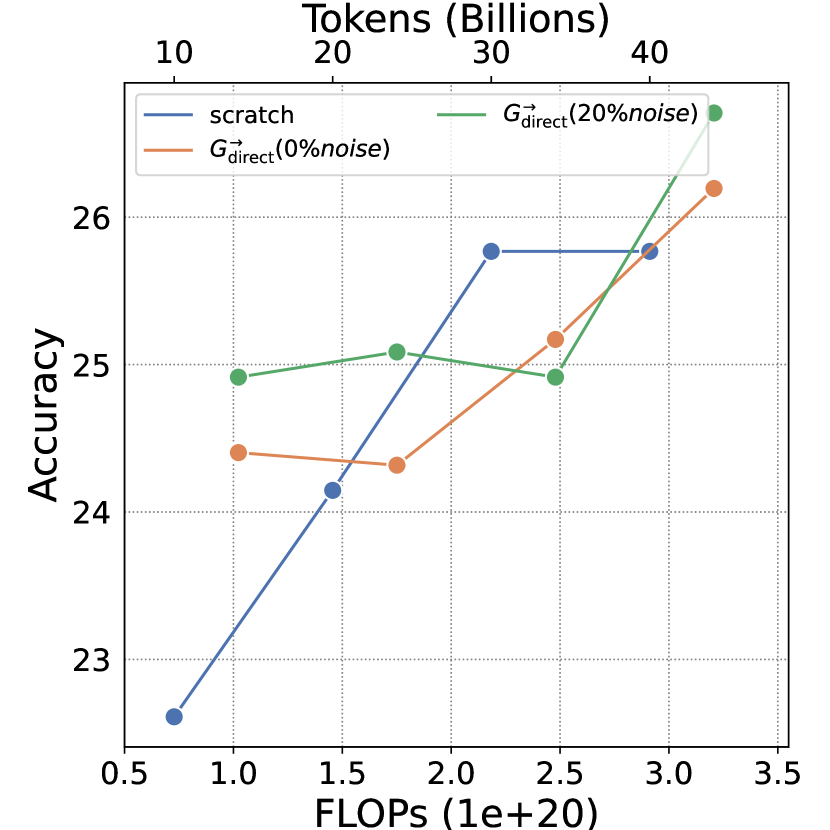
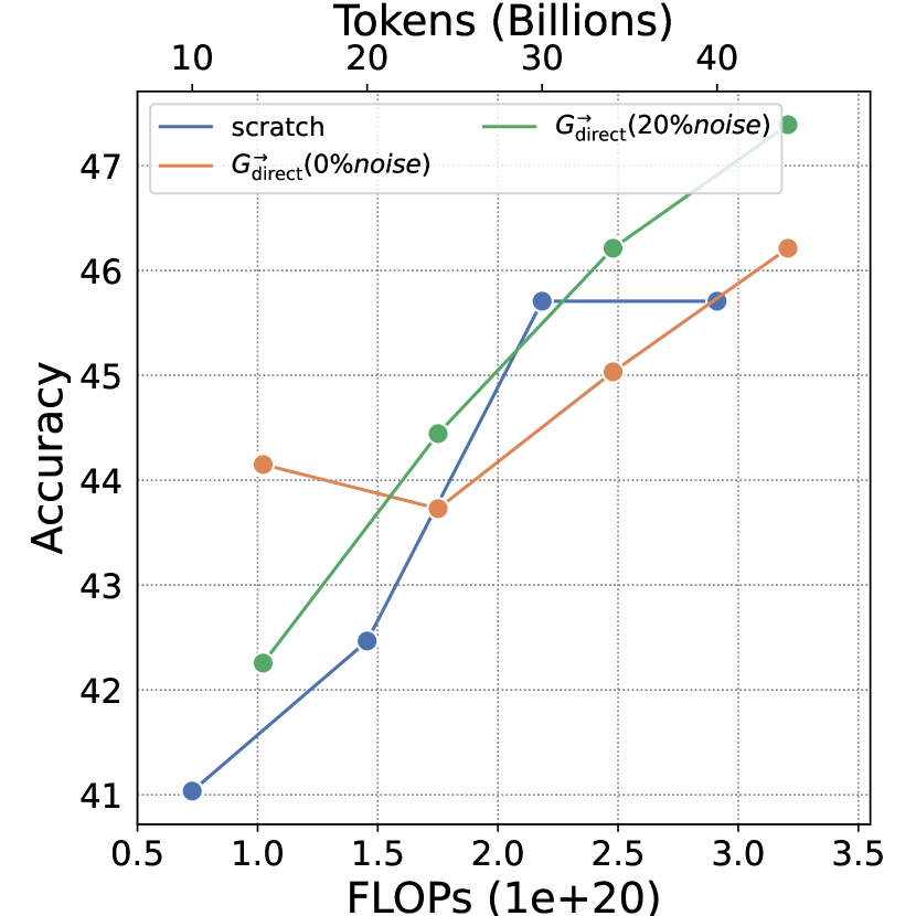
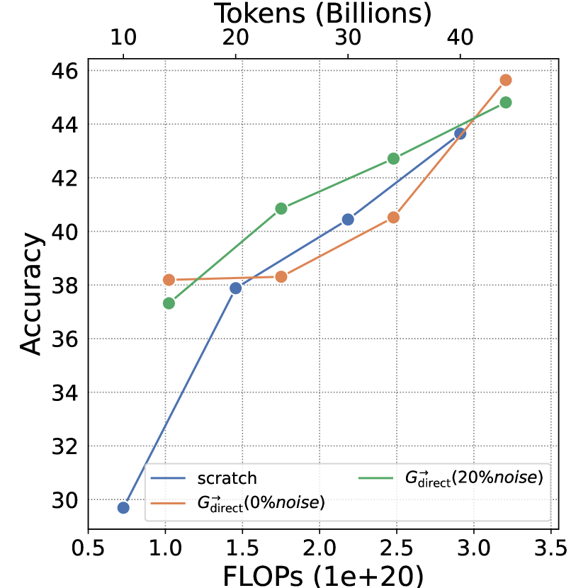
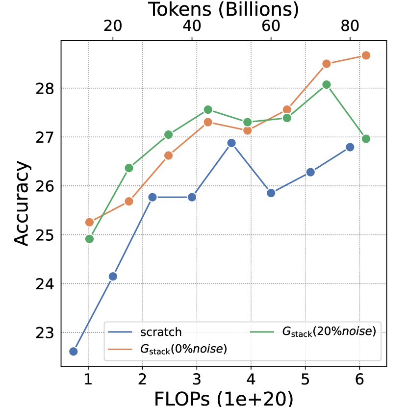
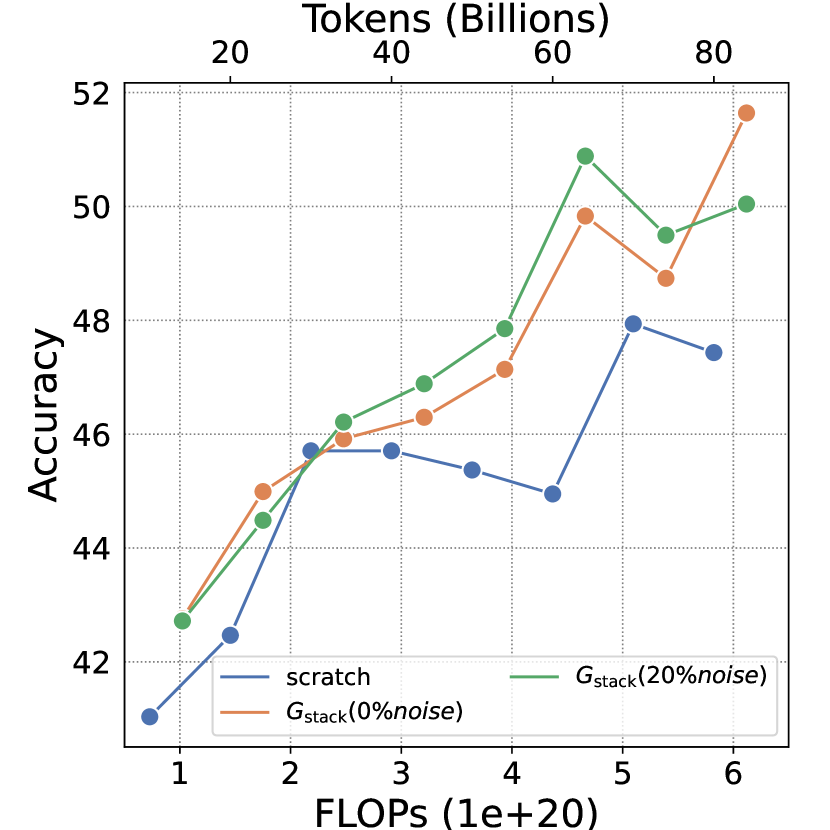
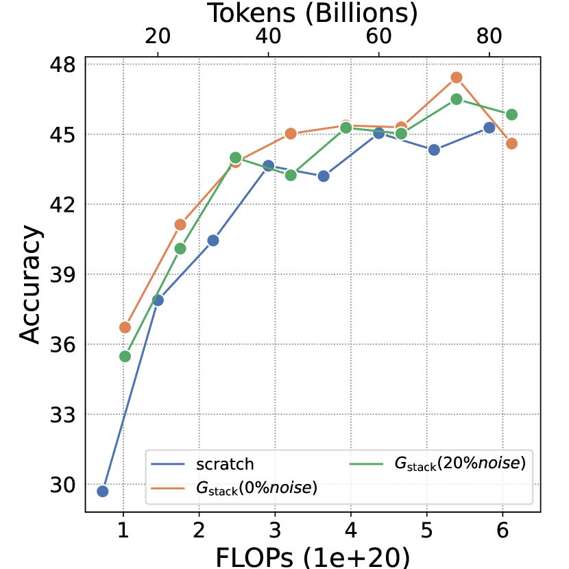
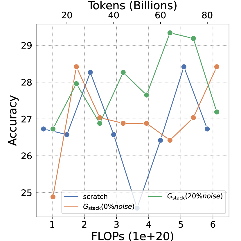
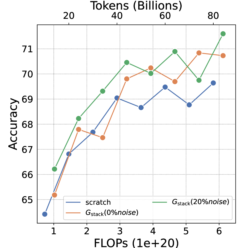
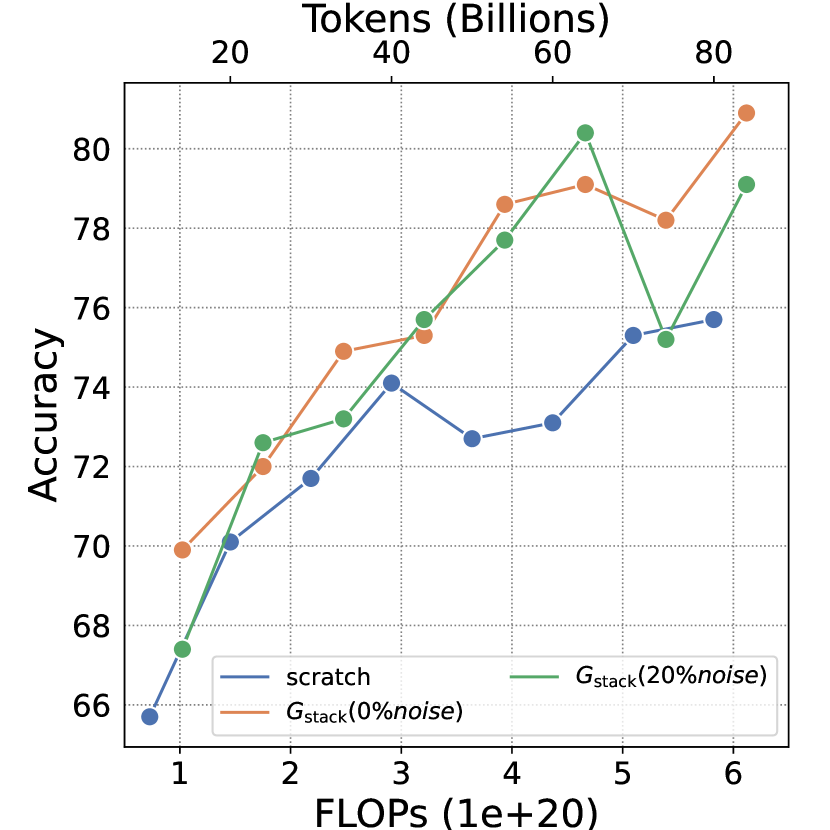
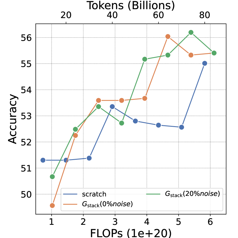
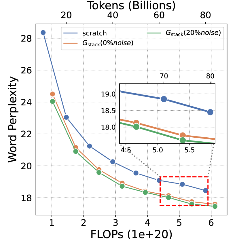
We find it intriguing that our approach, which violates FP, emerges as the most effective in our study. To further investigate, we conduct a simple ablation study to break FP by introducing noise on the strict-FP operator . We initialize the new neurons by a weighted combination of two sets of parameters: those from and those from random initialization. The weighting factor is controlled by a noise ratio. Our findings are intriguing. After 40B tokens training, adding 20% noise outperforms original by 0.27 on the Wikitext PPL and 0.41 on the average accuracy score.
We also add noise for . When we add 20% noise, our LLM performs slightly better than the no-noise model. However, when the noise level exceeds 20%, the performance significantly deteriorates. These results indicate that function preservation may not be the sole determining factor for model growth. In other words, exploring ways to accelerate the training of larger models and strict preserving function during growth might represent two overlapping yet distinct research directions. The experimental details are provided in the Appendix I.2.
6 Conclusion
This work empirically explores model growth approaches for efficient LLM pre-training. We address three key challenges of current model growth research for efficient LLM pre-training. We first comprehensively evaluate model growth techniques into four atomic operators and explore depthwise growth beats all other methods and baselines in various evaluations. We next address concerns about the scalability of by extending the model and training data scales. Furthermore, we systematically analyze the usage of the operator, focusing on growth timing and growth factor. Based on this analysis, we formalize a set of guidelines for effectively utilizing the operator. In addition, we provide in-depth discussions and comprehensive ablation studies of , shedding light on the broader implications of our work.
7 Limitations
While our work has demonstrated remarkable potential, three limitations deserve further attention. One limitation is the constraint of computation resources. For example, we only compare two sets of growth factor configurations, which limits the capacity to derive a formula for determining the optimal growth factor . Another limitation of our work is the focus on relatively simple operator choices, where we prioritize simplicity over exploring more sophisticated strategies. For instance, we do not investigate the multi-step growth or dynamic modifications to the training process, such as adjusting the learning rate during continual pre-training. Lastly, although this study’s scope is an empirical exploration and the content is self-contained, there is a lack of theoretical insights into the success of in LLM pre-training. Nonetheless, we will release all LLM checkpoints to facilitate the community’s investigation into the theoretical principles behind our observations.
References
- [1] Tom B. Brown, Benjamin Mann, Nick Ryder, Melanie Subbiah, Jared Kaplan, Prafulla Dhariwal, Arvind Neelakantan, Pranav Shyam, Girish Sastry, Amanda Askell, Sandhini Agarwal, Ariel Herbert-Voss, Gretchen Krueger, Tom Henighan, Rewon Child, Aditya Ramesh, Daniel M. Ziegler, Jeffrey Wu, Clemens Winter, Christopher Hesse, Mark Chen, Eric Sigler, Mateusz Litwin, Scott Gray, Benjamin Chess, Jack Clark, Christopher Berner, Sam McCandlish, Alec Radford, Ilya Sutskever, and Dario Amodei. Language models are few-shot learners, 2020.
- [2] Jason Wei, Yi Tay, Rishi Bommasani, Colin Raffel, Barret Zoph, Sebastian Borgeaud, Dani Yogatama, Maarten Bosma, Denny Zhou, Donald Metzler, Ed H. Chi, Tatsunori Hashimoto, Oriol Vinyals, Percy Liang, Jeff Dean, and William Fedus. Emergent abilities of large language models, 2022.
- [3] Jared Kaplan, Sam McCandlish, Tom Henighan, Tom B. Brown, Benjamin Chess, Rewon Child, Scott Gray, Alec Radford, Jeffrey Wu, and Dario Amodei. Scaling laws for neural language models, 2020.
- [4] Jordan Hoffmann, Sebastian Borgeaud, Arthur Mensch, Elena Buchatskaya, Trevor Cai, Eliza Rutherford, Diego de Las Casas, Lisa Anne Hendricks, Johannes Welbl, Aidan Clark, Tom Hennigan, Eric Noland, Katie Millican, George van den Driessche, Bogdan Damoc, Aurelia Guy, Simon Osindero, Karen Simonyan, Erich Elsen, Jack W. Rae, Oriol Vinyals, and Laurent Sifre. Training compute-optimal large language models, 2022.
- [5] Ibrahim Alabdulmohsin, Behnam Neyshabur, and Xiaohua Zhai. Revisiting neural scaling laws in language and vision, 2022.
- [6] Mengwei Xu, Wangsong Yin, Dongqi Cai, Rongjie Yi, Daliang Xu, Qipeng Wang, Bingyang Wu, Yihao Zhao, Chen Yang, Shihe Wang, Qiyang Zhang, Zhenyan Lu, Li Zhang, Shangguang Wang, Yuanchun Li, Yunxin Liu, Xin Jin, and Xuanzhe Liu. A survey of resource-efficient llm and multimodal foundation models, 2024.
- [7] AI@Meta. Llama 3 model card, 2024.
- [8] Carole-Jean Wu, Ramya Raghavendra, Udit Gupta, Bilge Acun, Newsha Ardalani, Kiwan Maeng, Gloria Chang, Fiona Aga Behram, James Huang, Charles Bai, Michael Gschwind, Anurag Gupta, Myle Ott, Anastasia Melnikov, Salvatore Candido, David Brooks, Geeta Chauhan, Benjamin Lee, Hsien-Hsin S. Lee, Bugra Akyildiz, Maximilian Balandat, Joe Spisak, Ravi Jain, Mike Rabbat, and Kim Hazelwood. Sustainable ai: Environmental implications, challenges and opportunities, 2022.
- [9] Alex de Vries. The growing energy footprint of artificial intelligence. Joule, 7(10):2191–2194, 2023.
- [10] Cheng Chen, Yichun Yin, Lifeng Shang, Xin Jiang, Yujia Qin, Fengyu Wang, Zhi Wang, Xiao Chen, Zhiyuan Liu, and Qun Liu. bert2bert: Towards reusable pretrained language models. arXiv preprint arXiv:2110.07143, 2021.
- [11] Linyuan Gong, Di He, Zhuohan Li, Tao Qin, Liwei Wang, and Tieyan Liu. Efficient training of bert by progressively stacking. In International conference on machine learning, pages 2337–2346. PMLR, 2019.
- [12] Cheng Yang, Shengnan Wang, Chao Yang, Yuechuan Li, Ru He, and Jingqiao Zhang. Progressively stacking 2.0: A multi-stage layerwise training method for bert training speedup. arXiv preprint arXiv:2011.13635, 2020.
- [13] Peihao Wang, Rameswar Panda, Lucas Torroba Hennigen, Philip Greengard, Leonid Karlinsky, Rogerio Feris, David Daniel Cox, Zhangyang Wang, and Yoon Kim. Learning to grow pretrained models for efficient transformer training. arXiv preprint arXiv:2303.00980, 2023.
- [14] Yite Wang, Jiahao Su, Hanlin Lu, Cong Xie, Tianyi Liu, Jianbo Yuan, Haibin Lin, Ruoyu Sun, and Hongxia Yang. Lemon: Lossless model expansion, 2023.
- [15] Sheng Shen, Pete Walsh, Kurt Keutzer, Jesse Dodge, Matthew Peters, and Iz Beltagy. Staged training for transformer language models. In International Conference on Machine Learning, pages 19893–19908. PMLR, 2022.
- [16] Albert Q. Jiang, Alexandre Sablayrolles, Arthur Mensch, Chris Bamford, Devendra Singh Chaplot, Diego de las Casas, Florian Bressand, Gianna Lengyel, Guillaume Lample, Lucile Saulnier, Lélio Renard Lavaud, Marie-Anne Lachaux, Pierre Stock, Teven Le Scao, Thibaut Lavril, Thomas Wang, Timothée Lacroix, and William El Sayed. Mistral 7b, 2023.
- [17] Xiang Li, Yiqun Yao, Xin Jiang, Xuezhi Fang, Xuying Meng, Siqi Fan, Peng Han, Jing Li, Li Du, Bowen Qin, Zheng Zhang, Aixin Sun, and Yequan Wang. Flm-101b: An open llm and how to train it with $100k budget, 2023.
- [18] Utku Evci, Bart van Merrienboer, Thomas Unterthiner, Max Vladymyrov, and Fabian Pedregosa. Gradmax: Growing neural networks using gradient information. arXiv preprint arXiv:2201.05125, 2022.
- [19] Yiqun Yao, Zheng Zhang, Jing Li, and Yequan Wang. Masked structural growth for 2x faster language model pre-training, 2024.
- [20] Hugo Touvron, Louis Martin, Kevin Stone, Peter Albert, Amjad Almahairi, Yasmine Babaei, Nikolay Bashlykov, Soumya Batra, Prajjwal Bhargava, Shruti Bhosale, Dan Bikel, Lukas Blecher, Cristian Canton Ferrer, Moya Chen, Guillem Cucurull, David Esiobu, Jude Fernandes, Jeremy Fu, Wenyin Fu, Brian Fuller, Cynthia Gao, Vedanuj Goswami, Naman Goyal, Anthony Hartshorn, Saghar Hosseini, Rui Hou, Hakan Inan, Marcin Kardas, Viktor Kerkez, Madian Khabsa, Isabel Kloumann, Artem Korenev, Punit Singh Koura, Marie-Anne Lachaux, Thibaut Lavril, Jenya Lee, Diana Liskovich, Yinghai Lu, Yuning Mao, Xavier Martinet, Todor Mihaylov, Pushkar Mishra, Igor Molybog, Yixin Nie, Andrew Poulton, Jeremy Reizenstein, Rashi Rungta, Kalyan Saladi, Alan Schelten, Ruan Silva, Eric Michael Smith, Ranjan Subramanian, Xiaoqing Ellen Tan, Binh Tang, Ross Taylor, Adina Williams, Jian Xiang Kuan, Puxin Xu, Zheng Yan, Iliyan Zarov, Yuchen Zhang, Angela Fan, Melanie Kambadur, Sharan Narang, Aurelien Rodriguez, Robert Stojnic, Sergey Edunov, and Thomas Scialom. Llama 2: Open foundation and fine-tuned chat models, 2023.
- [21] Jean Kaddour, Oscar Key, Piotr Nawrot, Pasquale Minervini, and Matt J. Kusner. No train no gain: Revisiting efficient training algorithms for transformer-based language models, 2023.
- [22] Leo Gao, Jonathan Tow, Baber Abbasi, Stella Biderman, Sid Black, Anthony DiPofi, Charles Foster, Laurence Golding, Jeffrey Hsu, Alain Le Noac’h, Haonan Li, Kyle McDonell, Niklas Muennighoff, Chris Ociepa, Jason Phang, Laria Reynolds, Hailey Schoelkopf, Aviya Skowron, Lintang Sutawika, Eric Tang, Anish Thite, Ben Wang, Kevin Wang, and Andy Zou. A framework for few-shot language model evaluation, 12 2023.
- [23] Scott Fahlman and Christian Lebiere. The cascade-correlation learning architecture. In D. Touretzky, editor, Advances in Neural Information Processing Systems, volume 2. Morgan-Kaufmann, 1989.
- [24] Scott E. Fahlman. The recurrent cascade-correlation architecture. In Neural Information Processing Systems, 1990.
- [25] Steven Gutstein, Olac Fuentes, and Eric A. Freudenthal. Knowledge transfer in deep convolutional neural nets. In Int. J. Artif. Intell. Tools, 2007.
- [26] Tianqi Chen, Ian Goodfellow, and Jonathon Shlens. Net2net: Accelerating learning via knowledge transfer. arXiv preprint arXiv:1511.05641, 2015.
- [27] Jacob Devlin, Ming-Wei Chang, Kenton Lee, and Kristina Toutanova. Bert: Pre-training of deep bidirectional transformers for language understanding, 2019.
- [28] Lemeng Wu, Bo Liu, Peter Stone, and Qiang Liu. Firefly neural architecture descent: a general approach for growing neural networks, 2021.
- [29] Xin Yuan, Pedro Savarese, and Michael Maire. Accelerated training via incrementally growing neural networks using variance transfer and learning rate adaptation, 2023.
- [30] Denis Paperno, Germán Kruszewski, Angeliki Lazaridou, Quan Ngoc Pham, Raffaella Bernardi, Sandro Pezzelle, Marco Baroni, Gemma Boleda, and Raquel Fernández. The lambada dataset: Word prediction requiring a broad discourse context, 2016.
- [31] Peter Clark, Isaac Cowhey, Oren Etzioni, Tushar Khot, Ashish Sabharwal, Carissa Schoenick, and Oyvind Tafjord. Think you have solved question answering? try arc, the ai2 reasoning challenge, 2018.
- [32] Jian Liu, Leyang Cui, Hanmeng Liu, Dandan Huang, Yile Wang, and Yue Zhang. Logiqa: A challenge dataset for machine reading comprehension with logical reasoning, 2020.
- [33] Yonatan Bisk, Rowan Zellers, Ronan Le Bras, Jianfeng Gao, and Yejin Choi. Piqa: Reasoning about physical commonsense in natural language, 2019.
- [34] Johannes Welbl, Nelson F. Liu, and Matt Gardner. Crowdsourcing multiple choice science questions, 2017.
- [35] Keisuke Sakaguchi, Ronan Le Bras, Chandra Bhagavatula, and Yejin Choi. Winogrande: An adversarial winograd schema challenge at scale, 2019.
- [36] Stephen Merity, Caiming Xiong, James Bradbury, and Richard Socher. Pointer sentinel mixture models, 2016.
- [37] Wayne Xin Zhao, Kun Zhou, Junyi Li, Tianyi Tang, Xiaolei Wang, Yupeng Hou, Yingqian Min, Beichen Zhang, Junjie Zhang, Zican Dong, Yifan Du, Chen Yang, Yushuo Chen, Zhipeng Chen, Jinhao Jiang, Ruiyang Ren, Yifan Li, Xinyu Tang, Zikang Liu, Peiyu Liu, Jian-Yun Nie, and Ji-Rong Wen. A survey of large language models, 2023.
- [38] Ziheng Jiang, Haibin Lin, Yinmin Zhong, Qi Huang, Yangrui Chen, Zhi Zhang, Yanghua Peng, Xiang Li, Cong Xie, Shibiao Nong, Yulu Jia, Sun He, Hongmin Chen, Zhihao Bai, Qi Hou, Shipeng Yan, Ding Zhou, Yiyao Sheng, Zhuo Jiang, Haohan Xu, Haoran Wei, Zhang Zhang, Pengfei Nie, Leqi Zou, Sida Zhao, Liang Xiang, Zherui Liu, Zhe Li, Xiaoying Jia, Jianxi Ye, Xin Jin, and Xin Liu. Megascale: Scaling large language model training to more than 10,000 gpus, 2024.
- [39] Zhengxiao Du, Aohan Zeng, Yuxiao Dong, and Jie Tang. Understanding emergent abilities of language models from the loss perspective, 2024.
- [40] Pauli Virtanen, Ralf Gommers, Travis E. Oliphant, Matt Haberland, Tyler Reddy, David Cournapeau, Evgeni Burovski, Pearu Peterson, Warren Weckesser, Jonathan Bright, Stéfan J. van der Walt, Matthew Brett, Joshua Wilson, K. Jarrod Millman, Nikolay Mayorov, Andrew R. J. Nelson, Eric Jones, Robert Kern, Eric Larson, C J Carey, İlhan Polat, Yu Feng, Eric W. Moore, Jake VanderPlas, Denis Laxalde, Josef Perktold, Robert Cimrman, Ian Henriksen, E. A. Quintero, Charles R. Harris, Anne M. Archibald, Antônio H. Ribeiro, Fabian Pedregosa, Paul van Mulbregt, Aditya Vijaykumar, Alessandro Pietro Bardelli, Alex Rothberg, Andreas Hilboll, Andreas Kloeckner, Anthony Scopatz, Antony Lee, Ariel Rokem, C. Nathan Woods, Chad Fulton, Charles Masson, Christian Häggström, Clark Fitzgerald, David A. Nicholson, David R. Hagen, Dmitrii V. Pasechnik, Emanuele Olivetti, Eric Martin, Eric Wieser, Fabrice Silva, Felix Lenders, Florian Wilhelm, G. Young, Gavin A. Price, Gert-Ludwig Ingold, Gregory E. Allen, Gregory R. Lee, Hervé Audren, Irvin Probst, Jörg P. Dietrich, Jacob Silterra, James T Webber, Janko Slavič, Joel Nothman, Johannes Buchner, Johannes Kulick, Johannes L. Schönberger, José Vinícius de Miranda Cardoso, Joscha Reimer, Joseph Harrington, Juan Luis Cano Rodríguez, Juan Nunez-Iglesias, Justin Kuczynski, Kevin Tritz, Martin Thoma, Matthew Newville, Matthias Kümmerer, Maximilian Bolingbroke, Michael Tartre, Mikhail Pak, Nathaniel J. Smith, Nikolai Nowaczyk, Nikolay Shebanov, Oleksandr Pavlyk, Per A. Brodtkorb, Perry Lee, Robert T. McGibbon, Roman Feldbauer, Sam Lewis, Sam Tygier, Scott Sievert, Sebastiano Vigna, Stefan Peterson, Surhud More, Tadeusz Pudlik, Takuya Oshima, Thomas J. Pingel, Thomas P. Robitaille, Thomas Spura, Thouis R. Jones, Tim Cera, Tim Leslie, Tiziano Zito, Tom Krauss, Utkarsh Upadhyay, Yaroslav O. Halchenko, and Yoshiki Vázquez-Baeza. Scipy 1.0: fundamental algorithms for scientific computing in python. Nature Methods, 17(3):261–272, February 2020.
- [41] Haihang Wu, Wei Wang, Tamasha Malepathirana, Damith Senanayake, Denny Oetomo, and Saman Halgamuge. When to grow? a fitting risk-aware policy for layer growing in deep neural networks, 2024.
- [42] Chengyue Wu, Yukang Gan, Yixiao Ge, Zeyu Lu, Jiahao Wang, Ye Feng, Ping Luo, and Ying Shan. Llama pro: Progressive llama with block expansion. arXiv preprint arXiv:2401.02415, 2024.
- [43] Dahyun Kim, Chanjun Park, Sanghoon Kim, Wonsung Lee, Wonho Song, Yunsu Kim, Hyeonwoo Kim, Yungi Kim, Hyeonju Lee, Jihoo Kim, et al. Solar 10.7 b: Scaling large language models with simple yet effective depth up-scaling. arXiv preprint arXiv:2312.15166, 2023.
- [44] Peiyuan Zhang, Guangtao Zeng, Tianduo Wang, and Wei Lu. Tinyllama: An open-source small language model, 2024.
- [45] Tri Dao, Daniel Y. Fu, Stefano Ermon, Atri Rudra, and Christopher Ré. Flashattention: Fast and memory-efficient exact attention with io-awareness, 2022.
- [46] Daria Soboleva, Faisal Al-Khateeb, Robert Myers, Jacob R Steeves, Joel Hestness, and Nolan Dey. SlimPajama: A 627B token cleaned and deduplicated version of RedPajama. https://www.cerebras.net/blog/slimpajama-a-627b-token-cleaned-and-deduplicated-version-of-redpajama, 2023.
- [47] Rowan Zellers, Ari Holtzman, Yonatan Bisk, Ali Farhadi, and Yejin Choi. Hellaswag: Can a machine really finish your sentence?, 2019.
- [48] Stephanie Lin, Jacob Hilton, and Owain Evans. Truthfulqa: Measuring how models mimic human falsehoods, 2022.
- [49] Dan Hendrycks, Collin Burns, Steven Basart, Andy Zou, Mantas Mazeika, Dawn Song, and Jacob Steinhardt. Measuring massive multitask language understanding, 2021.
- [50] Stella Biderman, Hailey Schoelkopf, Quentin Gregory Anthony, Herbie Bradley, Kyle O’Brien, Eric Hallahan, Mohammad Aflah Khan, Shivanshu Purohit, USVSN Sai Prashanth, Edward Raff, et al. Pythia: A suite for analyzing large language models across training and scaling. In International Conference on Machine Learning, pages 2397–2430. PMLR, 2023.
- [51] Leo Gao, Stella Biderman, Sid Black, Laurence Golding, Travis Hoppe, Charles Foster, Jason Phang, Horace He, Anish Thite, Noa Nabeshima, et al. The pile: An 800gb dataset of diverse text for language modeling. arXiv preprint arXiv:2101.00027, 2020.
Appendix A Details of Growth Operators
A.1 Four Growth Operators
A.1.1 Operator : Direct Derivation of Grown Parameters From Old Parameters
One intuitive strategy for expanding neural networks involves directly duplicating or splitting existing neurons. [11, 10, 14]. Unlike other growth operators, we distinguish between growth in terms of depth and width.
For width-wise expansion, the Net2Net technique and its transformer implementations [26, 10] involve splitting old neurons into two or more parts, with each splitting step achieving a=b+c. Depending on the specific splitting mechanism, there are two variations: even splitting and uneven splitting. The latter is proposed to address symmetry issues that arise when neurons are evenly split. In this paper, we adopt the approach of uneven splitting.
In the context of depth-wise expansion, a common practice is to duplicate layers, often referred to as “stacking” [11]. Therefore, we use the term to represent this operator. While this approach may appear to deviate from function preservation, it surprisingly yields a strong baseline.
A.1.2 Operator : Generation of New Parameters through Matrix Transformation
is an operator that learns a matrix transformation function to map small models to a larger one [13]. This operator is applicable to both width and depth expansion. Considering the original model with parameters , the target model with parameters , and as the hypernetwork for meta-learning, the training corpus is denoted as , and the language model loss is denoted as . Then, we optimize the following objective:
| (3) |
A.1.3 Operator : Setting New Parameters to 0
Setting new parameters to zero is often considered a simple method to achieve function preservation. However, optimizing networks with a significant number of zeros can present challenges. To tackle this issue, we adopt current practices that selectively zero out either the fan-in or fan-out parameters [15, 18, 14]. Specifically, for operator , during width growing, we zero out only the set of fan-out parameters for new neurons and randomly initialize the remaining ones. In the case of depthwise expansion, we zero out the final output layer of the newly-duplicated transformer blocks’ MultiHead Attention and MLP.
A.1.4 Operator : Random Initialization of New Parameters
This group follows the common practice of randomly initializing new parameters. In earlier attempts, old neurons were frozen after the growth process [12, 19]. However, to ensure function preservation, a recent study introduces a mask for new neurons after expansion [19]. This mask is gradually removed during ongoing training. We refer to this new approach as the growth operator .
A.2 Difference of Our Operators and Base Methods
The operators shares a similar setting to Lemon with minor variances due to Llama achitectures. is consistent with the methods LiGO, but with our own implementation. For , our approach aligns with Lemon in terms of depth, but differs from stagedTraining in width. Unlike stagedTraining, we do not double the width and assign zeros to the off-diagonal entries. Instead, our approach is more flexible; by zeroing out the submatrix in the bottom-left corner, we can extend it to any dimension. Our does not exhibit the “multi-hop” growth like MSG, instead, it grows “one-hop” directly to the target size. Our implementation of () differs from the algorithm employed in stackedBert. In stackedBert, a gradual growing technique is utilized, whereas our operator follows a more direct approach.
A.3 Details of
Embedding
Consider , and our goal is to expand it to , just copy some columns:
| (4) | |||||
| (5) | |||||
| (6) |
where is used to copy the embedding matrix .
Linear
Consider , target parameter , where , is defined as:
| (7) | |||||
| (8) | |||||
| (9) |
where is used for expanding the fan-in and is used for expanding the fan-out. To satisfy function preserving, we ensure that .
RMSNorm
For RMSNorm, a similar approach is adopted, consider parameter , expanded parameter :
| (10) | |||
| (11) |
Therefore, using the , it is not possible to achieve function preservation for RMSNorm
Depth ()
Consider a transformer with layers represented as . Our objective is to expand it to layers, where is a multiple of . We have various stacking forms for this purpose, such as (a) direct stacking: .
A.4 Details of
Embedding
Consider an embedding matrix . The operator expands it to with , where . Formally:
| (12) |
Therefore, give a token , the expanded embedding can be expressed as:
| (13) |
Linear
Consider parameter . expand it to , where and . Formally:
| (14) |
where are randomly initialized new parameters. Considering the input token before expansion, and the input after expansion :
| (15) |
| (16) | |||||
| (17) | |||||
| (18) | |||||
| (19) |
RMSNorm
Considering the parameter , expand it to like in Appendix A.5, because the input must be .
Depth
In depth, by retaining only the residual part and initializing the MHA and SwiGLU final linear projections to zero, the MHA and SwiGLU layers can achieve function preservation.
A.5 Details of
Embedding
Consider an embedding matrix . The goal of is to expand it to , where . Formally:
| (20) |
where represents randomly initialized new parameters. We use a mask to mask out the randomly initialized parts:
| (21) |
Therefore, for a token , the masked embedding can be expressed as:
| (22) |
Linear
Consider parameter . Our goal is to expand it to , where and . Formally:
| (23) |
where are randomly initialized new parameters. Considering the input token before expansion, and the input after expansion :
| (24) |
| (25) | |||||
| (26) |
To ensure that the expanded part of starts with zeros, we still utilize a mask:
| (27) |
| (28) |
RMSNorm
Considering the parameter , our objective is to expand it to , where is an undetermined coefficient and is a randomly initialized new parameter. Let the input be , then we have:
| (29) |
| (30) | |||||
| (31) | |||||
| (32) |
By observing equation 32, we can conclude that, to achieve function preservation, . Finally, we can conclude:
| (33) |
Depth
In depth, preserving only the residual part and masking the MHA and SwiGLU layers can achieve function preservation:
| (34) | |||
| (35) | |||
| (36) |
A.6 Details of
Using for width expansion, for the embedding layer , the parameter is defined as follows:
| (37) |
For Attention layer, where and , and RMSNorm , the parameters and , we have:
| (38) |
For MLP, where , , RMSNorm , the parameter , we have:
| (39) |
For the output head , we have:
| (40) |
Using for depth expansion, consider a transformer model with layers, we use to expand it to layers. For :
| (41) |
where represents learnable parameters. These parameters are used to expand the MHA vertically in depth. Similarly, for SwiGLU, we also perform expansion using a similar method. Formally, this can be written as:
| (42) |
where represents learnable parameters used for expanding SwiGLU in the depth.
Appendix B LLMs Framework and Training Details
Embedding
Consider a vocabulary size and embedding size . Then, the embedding matrix , and the one-hot vector for input tokens is denoted as , where is the sequence length. Formally, it can be written as:
| (43) |
for , where , it is guaranteed that .
Multi-Head Attention
Multi-Head Attention (MHA) consists of multiple attention heads, each of which computes its own self-attention. The results of these attention heads are then concatenated and projected to obtain the following output:
| (44) |
here, the input , parameters , , , and , where .
Feed Forward Network
The Feed Forward Network (FFN) consists of two linear layers and the activation function GeLU. Typically, the two linear layers first perform an up-projection to and then down-project back to the dimension . Therefore, FFN is defined as:
| (45) |
where the input , parameter and .
SwiGLU
LLaMA replaces the original FFN in the Transformer Decoder with SwiGLU, resulting in improved performance. SwiGLU consists of three linear layers and the swiglu activation function. It can be defined as:
| (46) |
where means the element-wise multiplication, the input , parameter , and .
RMSNorm
Before MHA, FFN, or SwiGLU, there is a layer of RMSNorm to enhance the stability of the model. Compared to LayerNorm, RMSNorm is simpler in form. Formally, it can be written as:
| (47) |
where , parameter .
B.1 LLMs Training with Growth Operator
B.2 Details of Speedup Calculation
We calculate speedup between operator and model pre-training by:
| (48) |
where and represent the FLOPs required by the scratch model and the model, respectively, to achieve the same loss.
B.3 Details of Training Settings
We use TinyLlama 333Apache-2.0 license [44] as our pre-training codebase. We employ FSDP (Fully Sharded DataParallel) along with FlashAttention [45] 2.0, and other acceleration techniques. We use the open-source dataset Slimpajama-627B 444The license of Slimpajama-627B includes: Common Crawl Foundation Terms of Use; C4 license; GitHub was limited to MIT, BSD, or Apache licenses only; Books: the_pile_books3 license and pg19 license; ArXiv Terms of Use; Wikipedia License; StackExchange license on the Internet Archive [46] for pre-training. The hyperparameters used for each model size are listed in Table 1. Our 7B model is trained over around 100B tokens per day on an NVIDIA Hopper cluster.
| Size | Context Length | Batch Size | max-LR | min-LR | Warmup Steps | LR Scheduler |
|---|---|---|---|---|---|---|
| 410M | 2048 | 2M tokens | 6e-4 | 6e-5 | 3000 | cosine |
| 1.1B | 2048 | 2M tokens | 3e-4 | 3e-5 | 3000 | cosine |
| 3B | 2048 | 2M tokens | 1.6e-4 | 1.6e-5 | 3000 | cosine |
| 7B | 2048 | 2M tokens | 1e-4 | 1e-5 | 3000 | cosine |
Appendix C Training Loss and Evaluation Results of Four Operators in both Depth and Width growth
We have two small (base) models, one trained with token count and another trained with token count .

Appendix D Evaluation Results of Scaling
D.1 3B
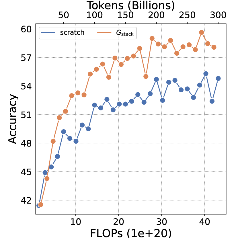
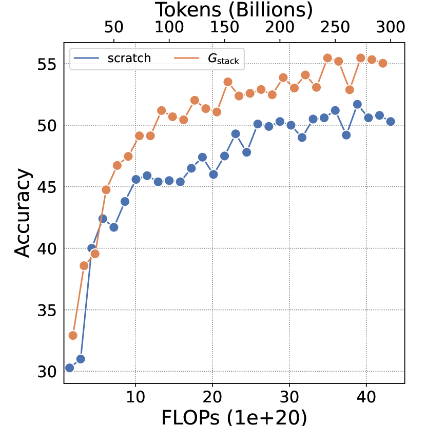
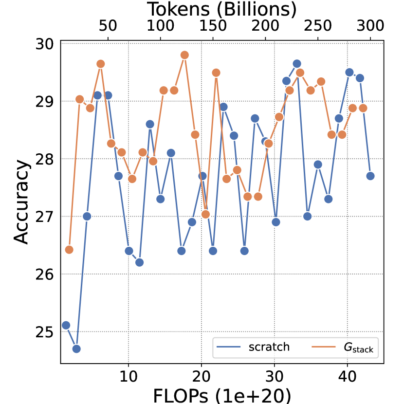
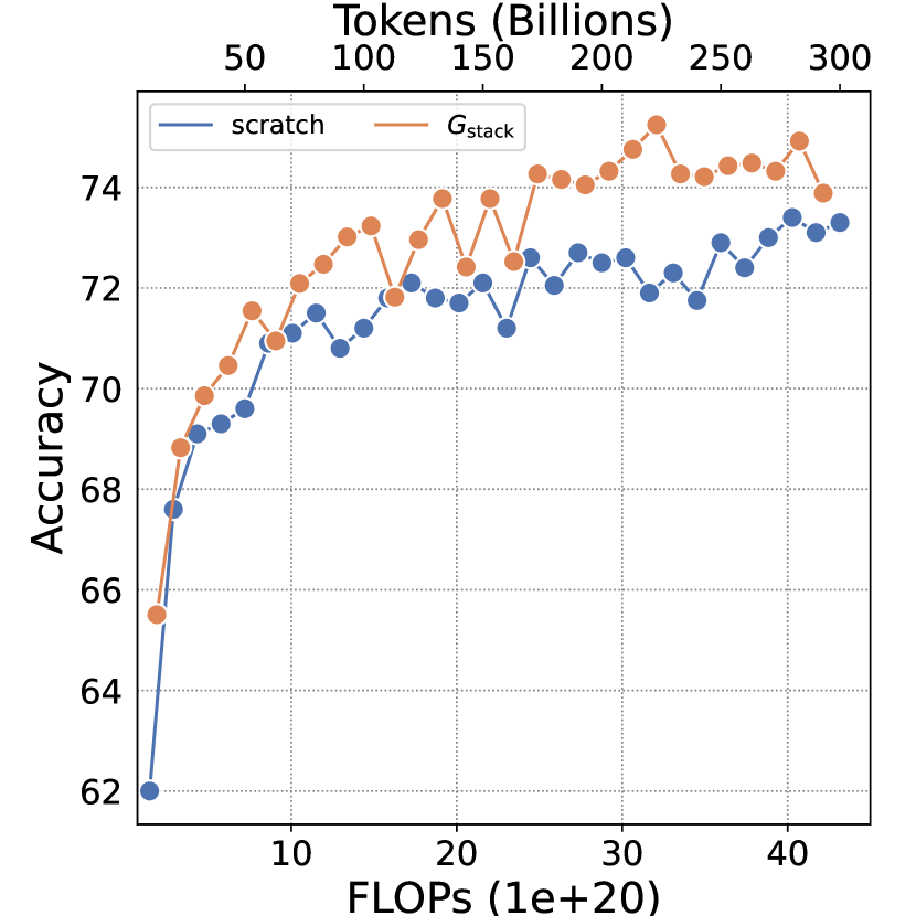
D.2 7B
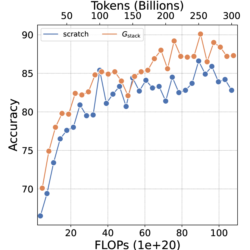
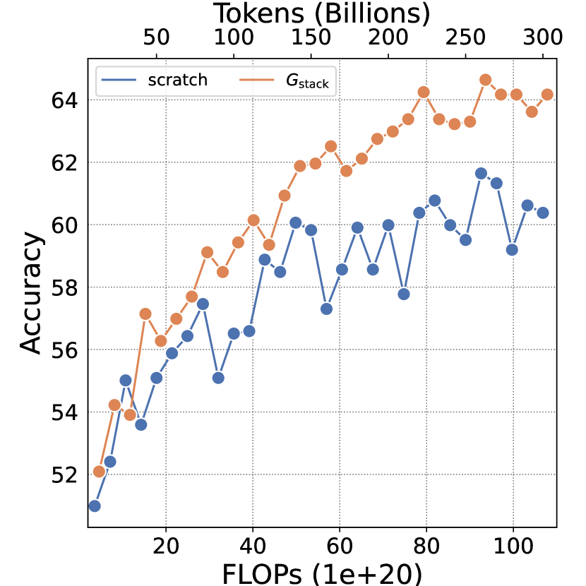
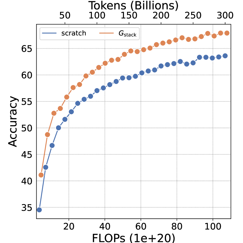
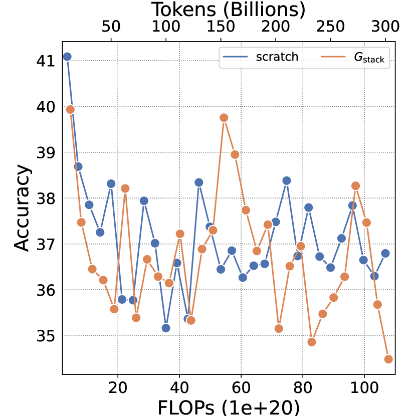
D.3 410M
D.4 Instruction Tuning Results on 3B
| Method | Tokens | Tuning | lambada | arc-c | arc-e | logiqa | piqa | sciq | winogrande | avg |
|---|---|---|---|---|---|---|---|---|---|---|
| scratch | 400B | \faTimes | 54.07 | 28.84 | 55.35 | 26.88 | 73.94 | 82.0 | 59.43 | 54.36 |
| \faCheck | 60.35 | 31.48 | 56.1 | 27.04 | 74.32 | 81.2 | 60.14 | 55.8 | ||
| \hdashline | 290B | \faTimes | 55.04 | 32.34 | 58.08 | 28.88 | 73.88 | 79.6 | 61.8 | 55.66 |
| \faCheck | 61.34 | 34.98 | 59.97 | 29.65 | 75.14 | 80.1 | 60.22 | 57.34 |
Appendix E Compare with Pythia and TinyLlama
In Table 3, we compare the harness evaluation results after training the model and the scratch model (Baseline) for 100B tokens with Pythia-1B [50] and TinyLlama-1.1B, which are trained on the same number of tokens. The comparative results indicate that our baseline performs normally, comparable to pythia-1B. Meanwhile, the model significantly outperforms both the baseline and pythia-1B, demonstrating the acceleration effect of on the pre-training process.
| Pythia-1B | TinyLlama-1.1B | -1.1B | Baseline-1.1B | |
|---|---|---|---|---|
| Datasets | Pile-300B [51] | Slimpajama-627B& Starcoder | Slimpajama-627B | Slimpajama-627B |
| Tokens | 100B | 103B | 100B | 100B |
| lambada | 53.52 | - | 48.20 | 47.87 |
| ARC-c | 25.59 | 24.32 | 29.18 | 27.21 |
| ARC-e | 47.26 | 44.91 | 54.25 | 48.86 |
| piqa | 69.31 | 67.30 | 71.98 | 69.64 |
| logiqa | 29.49 | - | 28.87 | 25.96 |
| sciq | 77.3 | - | 81.1 | 76.8 |
| winogrande | 51.22 | 53.28 | 56.03 | 54.53 |
| Avg. | 50.53 | - | 52.80 | 50.09 |
Appendix F Fitting Results for the Growth Factor
Although due to computational resource limitations, we only explore predicting given and on the 1.1B and 3B models, we still attempted to fit using equation:
| (49) |
In the equation 49, represents the number of target parameters, represents the growth factor. The fitting result is as follows:
| (50) |
We also visualize the fitted curves in Figure 22, but the results were mediocre due to the lack of data.
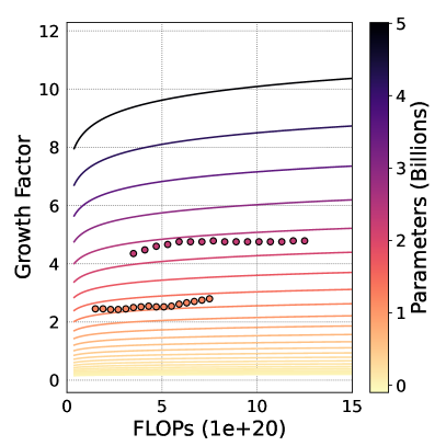
F.1 Stacking Law Guidelines For Llama Families
We give an example of empirical usage of by using the configurations of Llama2 and Llama3 families [20, 7] to show the estimated optimal base model training tokens and growth factor in Table 4.
| Model | N | D | ||
|---|---|---|---|---|
| Llama3-8B | 8B | 15T | 6.58B | 4 |
| Llama2-7B | 7B | 2T | 11.11B | 4 |
| Llama2-13B | 13B | 2T | 15.84B | 4 |
| Llama2-70B | 70B | 2T | 42.48B | 4 |
Appendix G Training Loss and Evaluation Results of “growth timing” and “growth factor”
G.1 “Growth Timing”
G.2 “Growth Factor”

Appendix H Discussion on “How to stack?” and Evaluation Results
H.1 Training Loss and Evaluation Results of Gradual Stack
H.2 Ablation: or (interpolation)
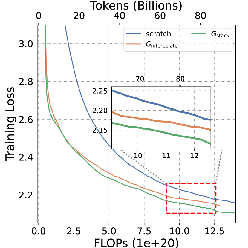
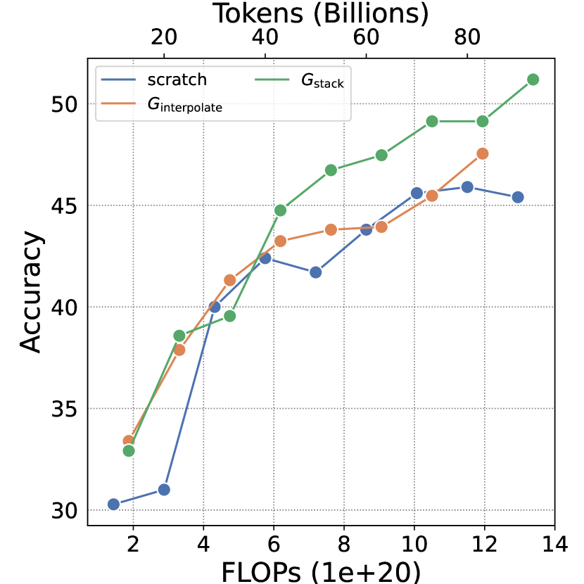
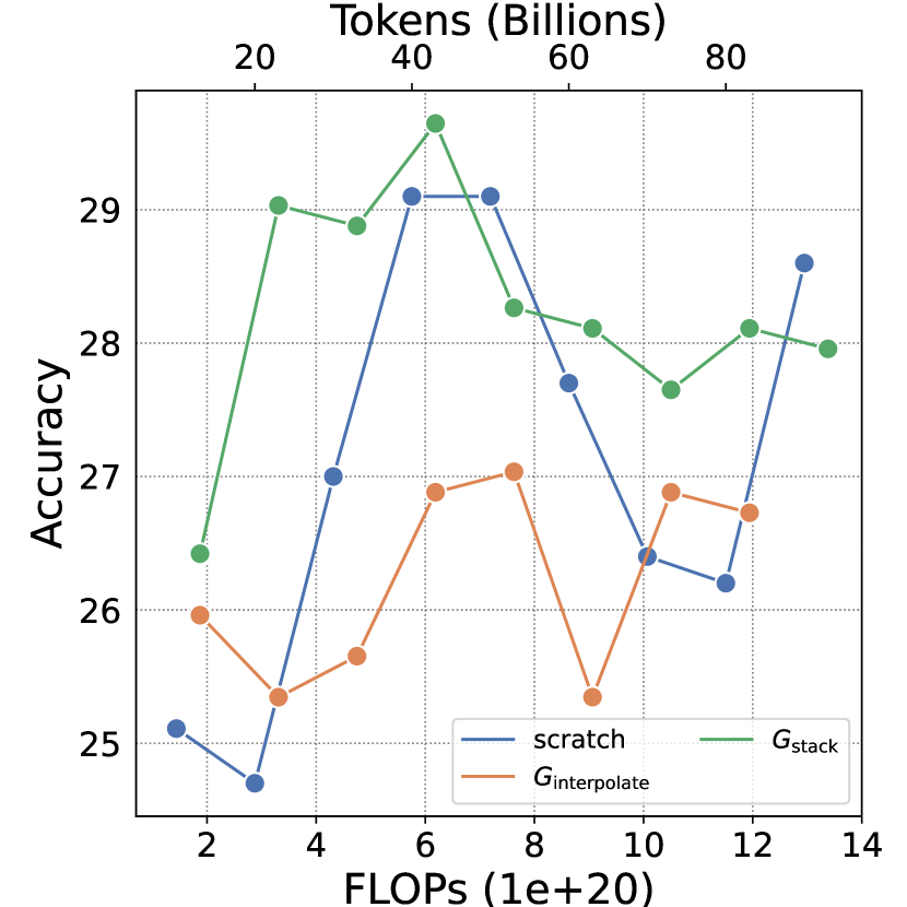
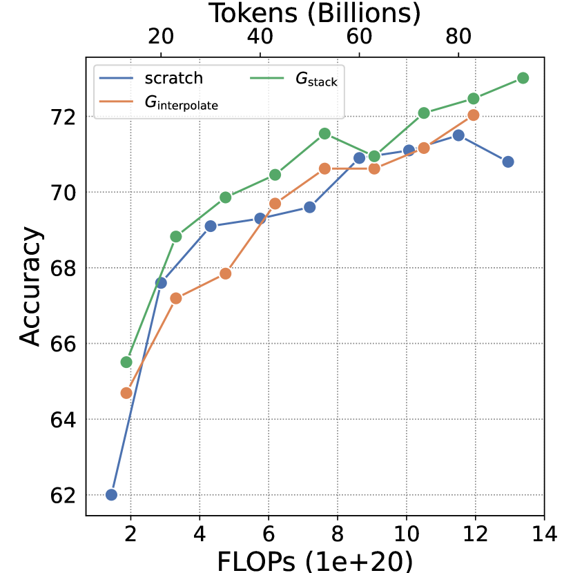
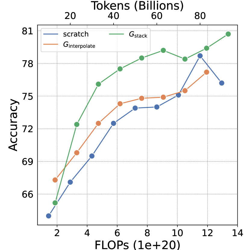
To investigate whether the connections between layers affect the performance of stacking, we conduct a comparison of two approaches for stacking small models into larger ones. We explore two approaches for stacking small models into larger ones. The first approach involves taking the entire small model as a unit and directly stacking it, which can retain the connections between most layers. The second approach involves replicating and interleaving each layer in the small model, which almost break the connections. To measure the degree of retention of inter-layer connections after stacking, we define the connection rate :
| (51) |
where the is number of retained connections, the is number of all connections.
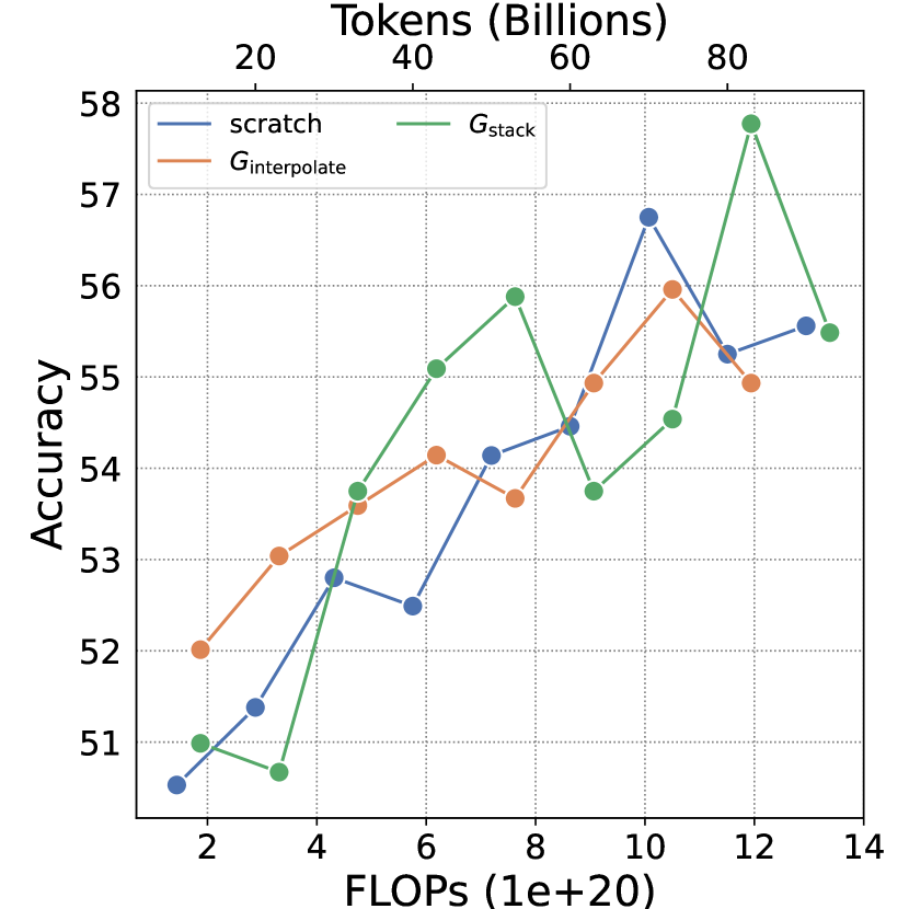
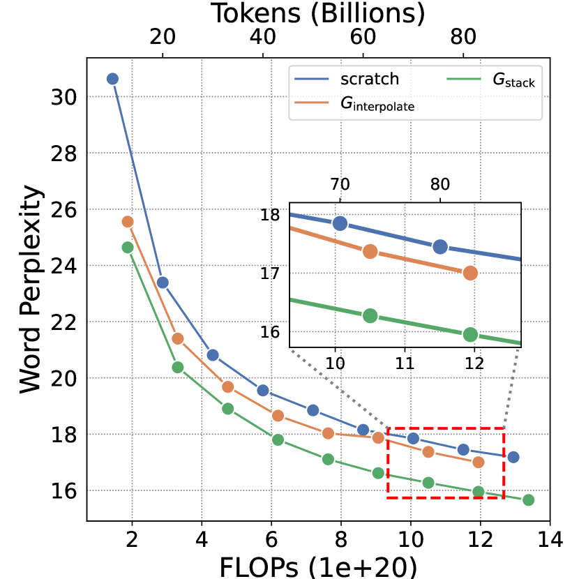
For example, if we had a small model with three layers, denoted as , and desired a model depth of 6, the first approach would result in , where its . The second approach would result in , where its .
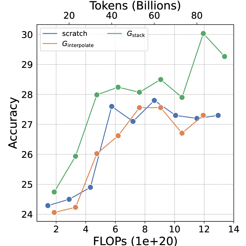
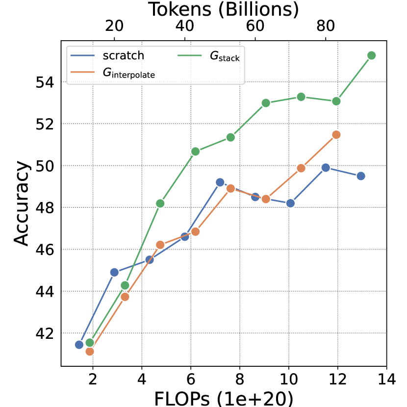
In our experiments, we stack a small model with 8 layers to a 24 layers target model. The growth timing is tokens and growing factor is . The of is and the of is . We report the training loss and standard NLP benchmarks average accuracy in Figure 35. At the beginning of training, interpolated stacking perform as well as stacking entire small model. However, as the training continues, the performance of interpolated stacking deteriorates.
Therefore, we can conclude that the higher the connection rate of stacking, the better the effect of stacking. In Appendix H.3, we continue to validate this conclusion.
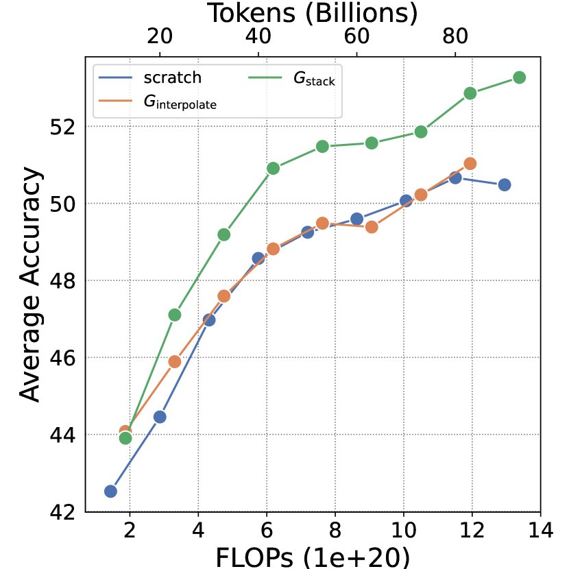
We also report the details of evaluation results about 8 standard NLP benchmarks.
H.3 Ablation: Partial Stacking
Partial stacking has been explored in LLMs like LlamaPro [42], Solar [43]. But their goal is to stack an off-the-shelf LLMs such as Llama2, while our aim is to accelerate LLM pre-training process.
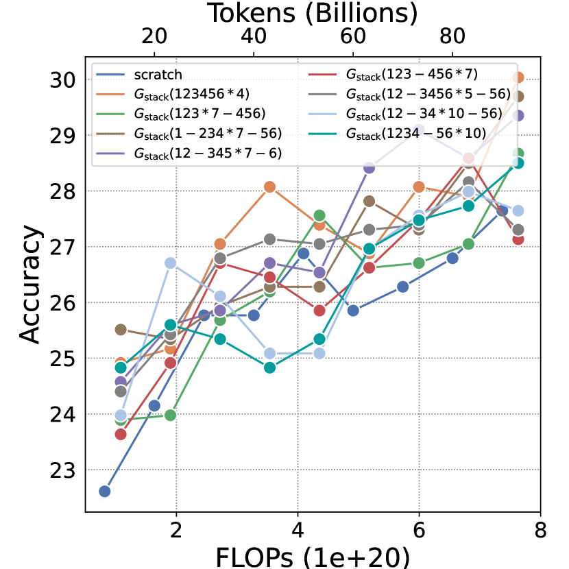
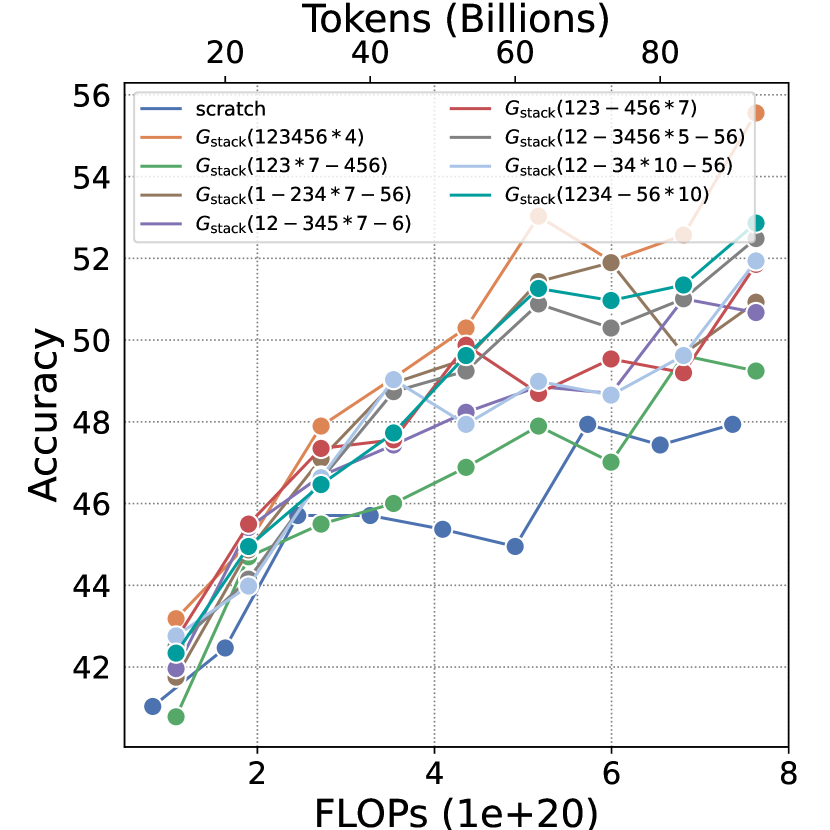
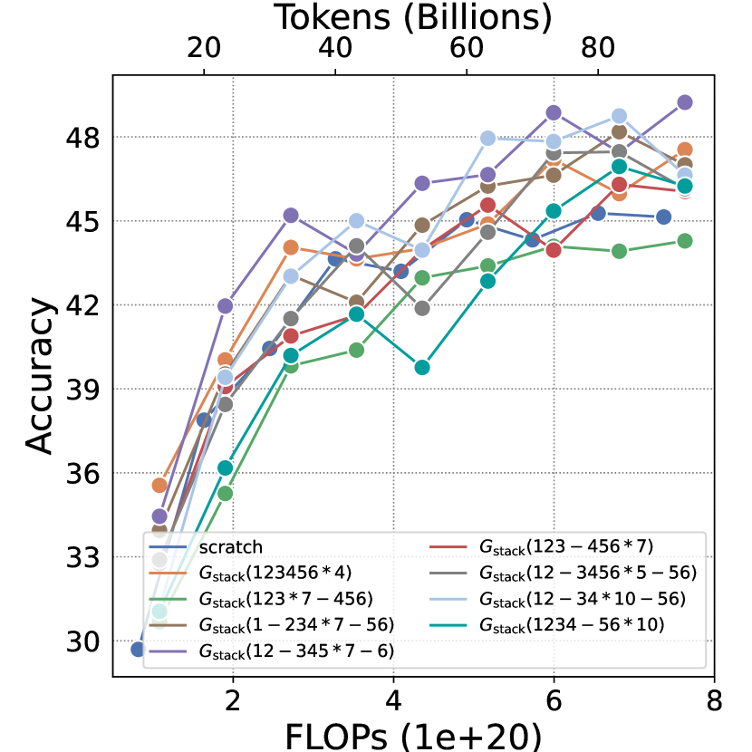
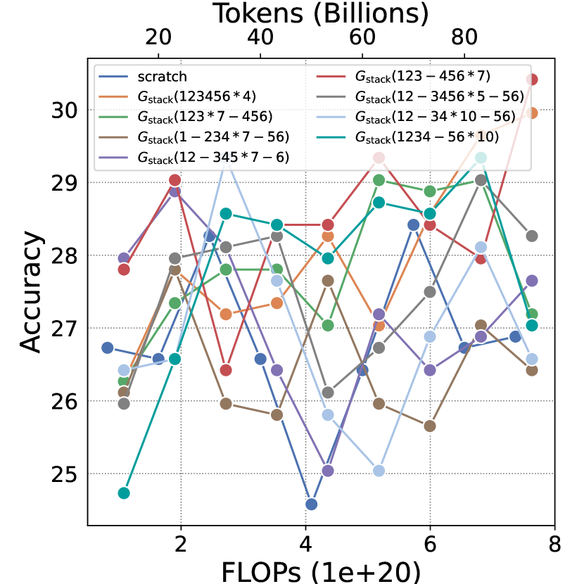
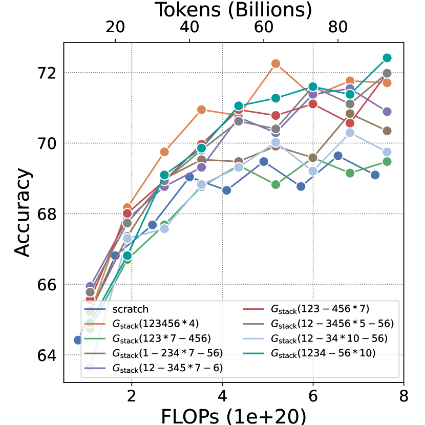
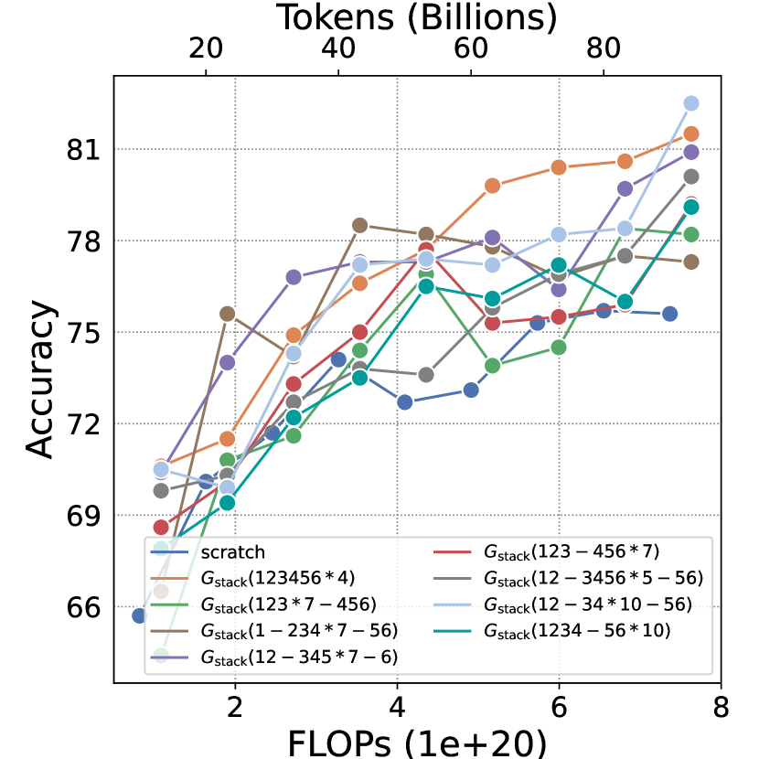
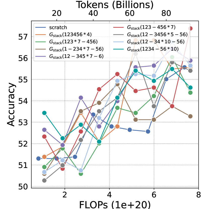
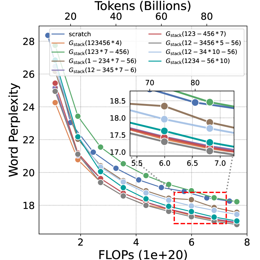
To explore stacking which layers of the small model can achieve the best performance, we conduct experiments on partial stacking. In our experiments, we stack a small model with 6 layers () to a 24 layers target model. We set growth timing tokens and growth factor . For simplicity, we use a format such as 1-234*7-56 to denote stacking 234 layers 7 times.

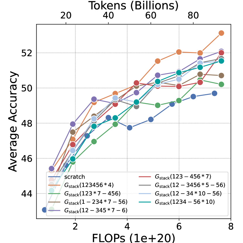
We report the training loss and standard NLP benchmarks average accuracy in Figure 37. By observing the loss curves in Figure 37(a), we can find that the eight partial stacking methods are clearly divided into three groups based on their loss. The first group, {123456*4, 12-3456*5-56, 12-345*7-6, 123-456*7}, achieves the best performance. The second group consisting of {1234-56*10, 12-34*10-56, 1-234*7-56}, performs just so-so. The third group, {123*7-456}, performs poorly, even worse than the baseline.
In Table 5, we summarize the eight partial stacking and calculate the of each partial stacking methods based on Equation 51.
For partial stacking, we conclude that: all middle back front. Meanwhile, when the stacked parts are the same, the larger the , the better the performance.
| Group | Method | Stacked parts | |
|---|---|---|---|
| First | 123456*4 | all | 87.0% |
| 12-3456*5-56 | middle-back | 78.3% | |
| 12-345*7-6 | middle-back | 74.0% | |
| 123-456*7 | back | 74.0% | |
| \hdashlineSecond | 1234-56*10 | back | 60.7% |
| 12-34*10-56 | middle | 60.7% | |
| 1-234*7-56 | front-middle | 74.0% | |
| \hdashlineThird | 123*7-456 | front | 74.0% |
Then, we report the evaluation results here.
Appendix I Details of Function Preserving
I.1 Function Preserving
Function preservation is a key concept that underlies diverse model growth approaches. It entails ensuring consistent output from a model, regardless of its expansion. Mathematically, let us define a function as and a growth operator as . The ultimate aim is to apply the operator to the function , thereby obtaining the target function denoted as . The core objective here is to maintain the model’s function to generate the same output for a given input. Formally,
| (52) |
I.2 Breaking Function Preserving by Adding Noise
For the down projection in SwiGLU and the output projection in MultiHeadAttention, we apply noise:
| (53) |
For the Embedding Layer and other Linear Layers, we apply noise:
| (54) |
Adding Noise on to Break FP
Training Loss And Evaluation Results on Adding Noise
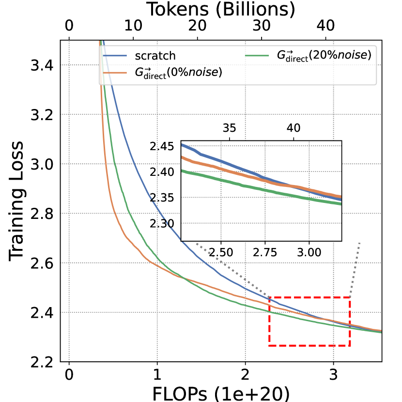
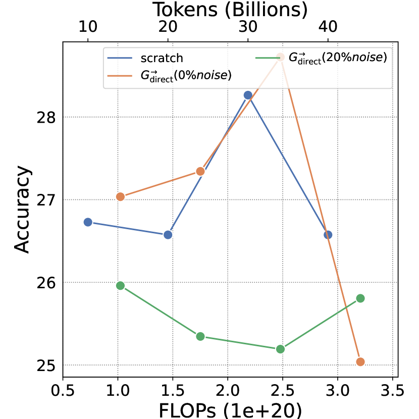
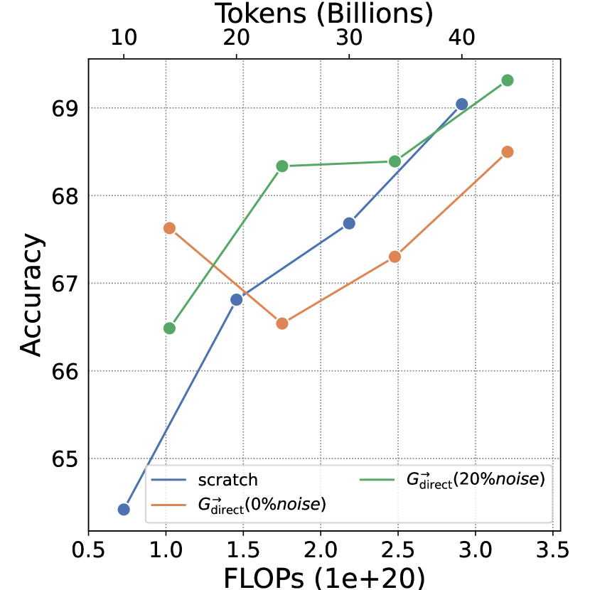
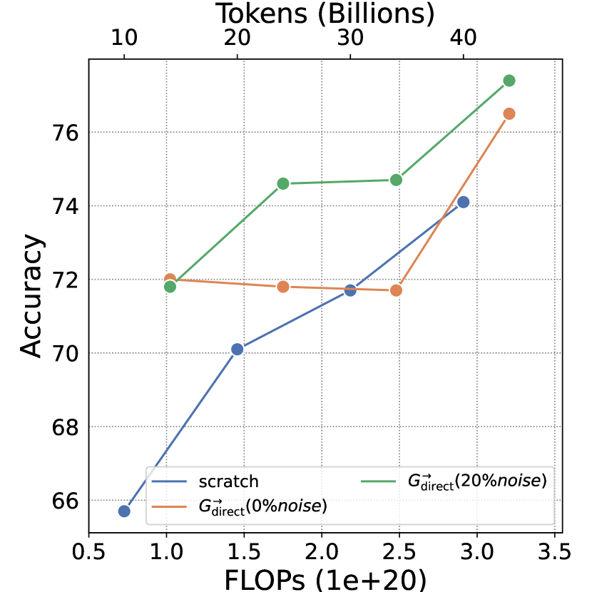
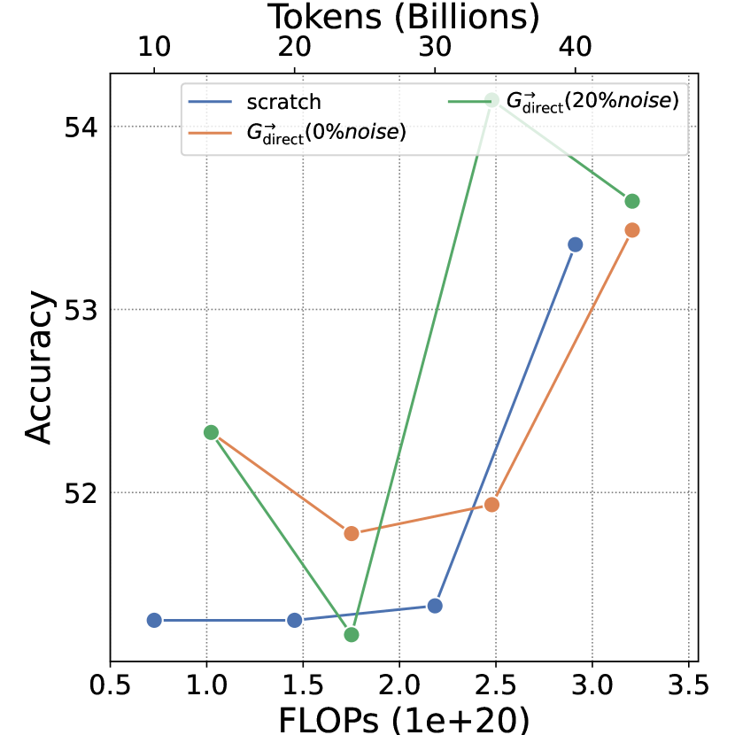
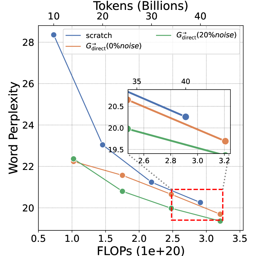
Adding Noise on
Since adding noise actually improve the performance, we also add noise on .
We stack an 8 layers small model to 24 layers, and then add noise with . We report training loss and standard NLP benchmarks average accuracy in Figure 41. Adding noise demonstrates an advantage in Training loss.

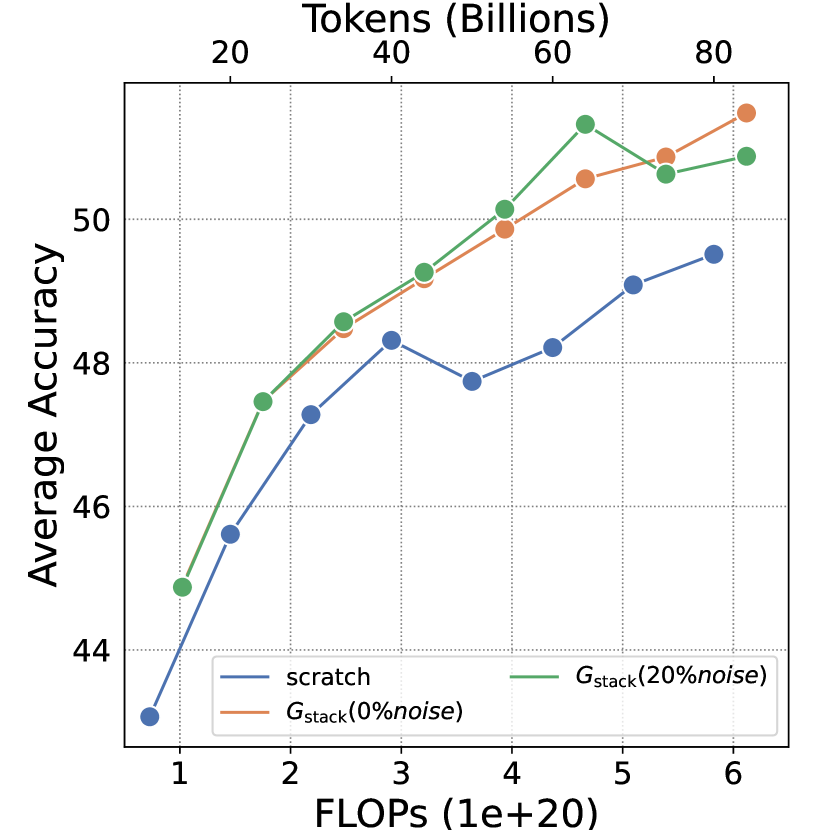
Details of the evaluation results are as follows:
Appendix J Societal Impacts
As a successful exploration for efficient LLM pre-training, our work has great potential to give positive societal impact towards sustainable AI. Nevertheless, as a common drawback for LLMs, there are also chances that our LLMs might be misused intentionally or uniintentionally.