Output-Constrained Decision Trees

Abstract

When there is a correlation between any pair of targets, one needs a prediction method that can handle vector-valued output. In this setting, multi-target learning is particularly important as it is widely used in various applications. This paper introduces new variants of decision trees that can handle not only multi-target output but also the constraints among the targets. We focus on the customization of conventional decision trees by adjusting the splitting criteria to handle the constraints and obtain feasible predictions. We present both an optimization-based exact approach and several heuristics, complete with a discussion on their respective advantages and disadvantages. To support our findings, we conduct a computational study to demonstrate and compare the results of the proposed approaches.

1 Introduction

Decision trees (DTs) play a fundamental role in machine learning and data science for several key reasons. Firstly, DTs have proven to be accurate predictive models in a wide range of applications. Moreover, the heuristic approaches used for their construction are computationally efficient, resulting in extremely fast training times. Accuracy and speed make them ideal for large datasets or real-time applications. Secondly, DTs, particularly those that are not too deep, are inherently explainable. By following the branches of such a trained tree, one can easily understand the logic behind the model’s predictions. This feature is particularly valuable in sectors where interpretability is critical, such as in healthcare or finance. Lastly, DTs serve as the base learners in powerful ensemble methods. These methods, which include techniques like random forests and gradient boosting, utilize numerous DTs to create robust and accurate predictive models.

When there is a correlation between any pair of targets, we need a prediction method that can handle vector-valued output. In this setting, multi-target learning is particularly important as it is widely used in fields such as forecasting, monitoring, manufacturing, and recommendation systems. DTs can easily be customized for handling multi-target regression by modifying the splitting criteria to handle vector predictions at each node.

Motivation.

Despite the wealth of existing literature on DTs, to the best of our knowledge, none consider cases where constraints exist among multiple targets. This is notable, as in many applications, decision-makers are aware of these constraints, and data analysts should impose them for feasible predictions.

As an illustrative example consider a dataset of students each with distinct attributes. This dataset also includes the grades of these students for five elective sophomore courses, represented as five-dimensional target vectors (training set). The goal is to predict the grades of the junior students should they choose to enroll in these elective courses (test set). To this end, one can train a DT and obtain the partitions of the sophomore students represented by the leaf nodes of the trained tree. Then, the prediction for a junior student is simply the average of the grades (mean vector) within the leaf node that she falls in. This leads to the prediction of five different grades, one for each course. However, it is essential to consider an additional constraint in our scenario: A student can enroll in a maximum of two out of the five elective courses. Consequently, if one continues to use the mean vector approach for prediction, it may not only yield inaccurate results but also infeasible predictions because of not accounting for this constraint. Interestingly, this erroneous estimation would also persist with many well-known DT training algorithms, since their estimation at a leaf node is also based on taking the mean or the median of the target vectors within the node. However, one may argue that growing a deeper DT may resolve the infeasibility issue as there will be fewer students at each leaf node. Even if we overlook the loss of interpretability due to the large size of such a tree, it is well-known that deep trees can easily overfit. Figure 1 shows our results with the grade prediction dataset (for details see, Section 3). The bar plot demonstrates that feasible predictions can be achieved with larger tree depths, but this comes with a significant decrease in accuracy as shown in the scatter plot. The scatter plot, on the other hand, shows that while shallow trees offer much better accuracy, most of their predictions are infeasible.

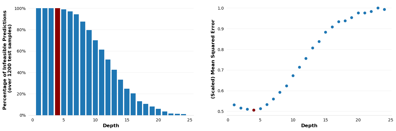
Figure 1: The results of the motivating example demonstrating the trade-off between accuracy and feasibility. The red circle in the right plot marks the depth of the tree which returns the lowest mean squared error value for the test set. The corresponding red bar in the left plot shows the corresponding percentage of infeasible predictions. The sample size is 4000.

Output-Constraints.

To obtain accurate and feasible predictions, we propose an optimization-based exact approach. This approach incorporates target constraints into the splitting procedure of common binary tree construction methods. Our approach ensures that the estimated target vector at each node meets the required constraints. However, we observe that the exact approach could have a lengthy computation time, especially for deep trees. To address this, we offer two heuristic approaches. These are based on using existing samples as predictions or relaxing the constraints with a penalty function at each split operation.

Up until now, our focus has been on regression problems. It is reasonable to question why we have not considered multi-target classification problems as well. The reason is, if the number of classes for each target and the number of targets are relatively small, we can assign a label to each feasible combination of target values. This approach effectively reduces the problem to a standard single-target classification problem, although possibly with many labels.

Related Work.

As machine learning methods improve in accuracy, they may still produce predictions and outcomes that lack physical consistency or feasibility, due to biases or data sparsity[23]. To overcome this challenge, hybrid methods that integrate optimization techniques with machine learning models have gained significant attention in recent years due to their ability to leverage the strengths of both approaches. One key aspect of hybrid approaches is their ability to handle constraints from various sources to enhance the feasibility and accuracy of machine learning methods. These constraints can originate from the dataset, user-defined specifications, or domain knowledge [16]. Such machine learning approaches with imposed constraints are developed as practical applications across different domains, such as mechanics [22], geomechanics [8], and electronics [14].

One of the earliest hybrid approaches was implemented by Lee and Kang [13], who introduced constraints to deep learning architectures to approximate ordinary and partial differential equations. This approach has laid the essentials of the general framework, called physics-informed neural networks by Raissi et al. [19], where constraints and boundary conditions are incorporated [20].

DTs also provide the ability to enforce constraints. Many hybrid DT approaches incorporate instance-level constraints to bind a subset of instances in generating meaningfully combined results. For instance, the clustering tree algorithm by Struyf and Džeroski [21] integrates domain knowledge to impose instance-level constraints such as ‘must-link’ and ‘cannot-link’ constraints. Additionally, DT methods have been developed to address adversarial examples, which can be considered as instance-level constraints [7, 5] or attribute-level constraints to assign several features to the predictors [16]. The work by Ben-David [1] was one of the first implementations of attribute-level constraints to impose monotonicity among the predictors of the model. Cardoso and Sousa [6] also developed a similar DT algorithm in an ordinal classification setting. To the best of our knowledge, our proposed approach is the first method designed to handle constraints among the target variables.

Contributions.

We introduce novel approaches to handle constraints among target variables in DTs. The first method lends itself to an optimization-based exact method that ensures the feasibility of predictions by incorporating target constraints into the splitting procedure of common binary tree construction methods. We also propose two heuristic methods. These methods offer practical solutions to the computation time issue that might be associated with the exact approach, especially for deep trees. We provide the technical details of our proposed methods, exploring their strengths, potential limitations, and the conditions under which they would perform sensibly. To validate our approaches, we provide a reproducible computational study using our publicly available implementation.

2 Output-Constrained Decision Trees

Suppose that we have the training dataset $\mathcal{D}=\{(\mbox{\boldmath{$x$}}_{i},\mbox{\boldmath{$y$}}_{i}):i\in\mathcal{I}_{\mathcal{D}}\}$ with $\mbox{\boldmath{$x$}}_{i}\in\mathbb{R}^{p}$ and $\mbox{\boldmath{$y$}}_{i}\in\mathbb{Y}\subseteq\mathbb{R}^{k}$ denoting the input vector and the target (output) vector for the data point $i$, respectively. The set $\mathbb{Y}$ shows the feasible set for the target vectors. It is important to observe that the target vector of each sample lies in $\mathbb{Y}$, and hence, they are also feasible.

A DT is grown by splitting the dataset into non-overlapping subsets recursively [4]. Each subset is represented by a node of the tree. The most common approach of tree construction uses binary splits; that is, at each iteration at most two child nodes, left ($\leftharpoonup$) and right ($\rightharpoonup$), are grown from a parent node. Let $\mathcal{N}\subseteq\mathcal{D}$ be the subset denoted by the parent node, and $\mathcal{I}_{\mathcal{N}}\subseteq\mathcal{I}_{\mathcal{D}}$ indicate the indices of the samples in that node. To obtain a pair of child nodes, a feature $j$ and a split value $v$ is selected to obtain the left and right index sets

$$\mathcal{I}^{\leftharpoonup}_{\mathcal{N}}(j,v)=\{i\in\mathcal{I}_{\mathcal{N}}:x_{ij}\leq v\}$$

and

$$\mathcal{I}^{\rightharpoonup}_{\mathcal{N}}(j,v)=\{i\in\mathcal{I}_{\mathcal{N}}:x_{ij}>v\},$$

respectively. Then, the gain by such a split is evaluated by

$$\alpha^{\leftharpoonup}_{\mathcal{N}}(j,v)\sum_{i\in\mathcal{I}^{\leftharpoonup}_{\mathcal{N}}(j,v)}\ell(\mbox{\boldmath{$y$}}_{\mathcal{N}},\mbox{\boldmath{$y$}}_{i})+\alpha^{\rightharpoonup}_{\mathcal{N}}(j,v)\sum_{i\in\mathcal{I}^{\rightharpoonup}_{\mathcal{N}}(j,v)}\ell(\mbox{\boldmath{$y$}}_{\mathcal{N}},\mbox{\boldmath{$y$}}_{i}),$$ (1)

where $\mbox{\boldmath{$y$}}_{\mathcal{N}}\in\mathbb{Y}$ is the prediction of the parent node, $\ell:\mathbb{R}^{k}\times\mathbb{R}^{k}\mapsto\mathbb{R}$ is the loss function, $\alpha^{\leftharpoonup}_{\mathcal{N}}(j,v)=\tfrac{|\mathcal{I}^{\leftharpoonup}_{\mathcal{N}}(j,v)|}{|\mathcal{I}_{\mathcal{N}}|}$ as well as $\alpha^{\rightharpoonup}_{\mathcal{N}}(j,v)=1-\alpha^{\leftharpoonup}_{\mathcal{N}}(j,v)$ are the scaling coefficients representing the proportional weights of the respective subsets. Among all possible splits, the one that achieves the largest gain is used to construct the child nodes. The splitting continues until one of the stopping conditions, such as reaching the maximum depth or the minimum number of samples in a node, is satisfied. Then, the samples in the last parent constitutes a leaf node. Considering the feasibility requirements on the predictions, the output vector $\mbox{\boldmath{$y$}}_{\mathcal{N}}$ of such a leaf node should be feasible; i.e., it belongs to the feasible set, $\mbox{\boldmath{$y$}}_{\mathcal{N}}\in\mathbb{Y}$.

2.1 Exact Approach

Almost all the loss functions (e.g., mean squared error, half Poisson deviance, mean absolute error) used in constructing binary DTs are separable. Moreover, the loss in the multi-target case is obtained by summing up individual losses for each target. Consider, for instance, the well-known mean squared error for which the prediction at a node with the subset $\mathcal{N}$ is given by

$$\mbox{\boldmath{$y$}}_{\mathcal{N}}=\arg\min_{\mbox{\boldmath{$y$}}\in\mathbb{Y}}~{}\frac{1}{|\mathcal{I}_{\mathcal{N}}|}\sum_{i\in\mathcal{I}_{\mathcal{N}}}\|\mbox{\boldmath{$y$}}-\mbox{\boldmath{$y$}}_{i}\|^{2}.$$

If there are no restrictions on the output vectors, i.e., $\mathbb{Y}=\mathbb{R}^{k}$, then it is not difficult to observe by simple differentiation that $\mbox{\boldmath{$y$}}_{\mathcal{N}}$ is the mean of the target vectors in $\mathcal{N}$ minimizing the subset variance. This is, in fact, the output of a node used by the well-known implementations, like scikit-learn [18]. The same holds for the half Poisson deviance loss function. In case of mean absolute error loss function, one can also show that the median of the target vectors in $\mathcal{N}$ becomes $\mbox{\boldmath{$y$}}_{\mathcal{N}}$ when $\mathbb{Y}=\mathbb{R}^{k}$. Hence, the median vector is the default node output in standard implementations evaluating the loss with mean absolute error. In fact, the following lemma shows that the mean and the median vectors are still the optimal choices when the constraints on the output vectors result in a convex feasible set.

Lemma 2.1

Let the feasible set $\mathbb{Y}$ be convex, then the following two statements are true:

1. If the loss function is the mean squared error or the Poission deviance, then the mean of the target vectors in a node minimizes the loss.

2. If the loss function is the mean absolute error, then the median of the target vectors in a node minimizes the loss.

Proof.

Recall that the mean and the median of the target vectors are both the unconstrained minimizers of the respective loss functions. The proof immediately follows from observing that both mean and median operations boil down to taking convex combinations of the feasible target vectors in the node. ∎

This lemma implies that a large class of feasible sets can be handled with standard DT implementations. For instance, simple bounds or, more generally, linear constraints on the target vectors lead to convex feasible sets. However, the same conclusion does not hold when the feasible set is not convex. Going back to our illustrative example of students, the grades naturally have lowest and highest values (say, 1 and 10), and if we use only these bounds as constraints, then any standard implementation returning the mean vector for each node output would not violate this constraint. However, if we also impose the selection restriction “at most two among five courses,” then we need auxiliary binary variables to represent this restriction as a constraint, and hence, the feasible set $\mathbb{Y}$ becomes non-convex. Formally,

$$\mathbb{Y}=\left\{\mbox{\boldmath{$y$}}\in\mathbb{R}^{5}:\sum_{t=1}^{5}z_{t}\leq 2,\ 0\leq y_{t}\leq 10z_{t},\text{ and }\ z_{t}\in\{0,1\}\text{ for }t=1,\dots,5\right\},$$ (2)

where the binary variable $z_{t}$ becomes one when the student receives a grade of $y_{t}$ for course $t$. Note that when $z_{t}$ is zero, then it also forces $y_{t}$ to become zero implying that the student did not select that course.

We can now state the formal prediction model that needs to be solved at each node:

$$\mbox{\boldmath{$y$}}_{\mathcal{N}}=\arg\min_{\mbox{\boldmath{$y$}}\in\mathbb{Y}}~{}\sum_{i\in\mathcal{I}_{\mathcal{N}}}\ell(\mbox{\boldmath{$y$}},\mbox{\boldmath{$y$}}_{i}),$$ (3)

where $\mathcal{I}_{\mathcal{N}}\subseteq\mathcal{I}_{\mathcal{D}}$ with $\mathcal{N}\subseteq\mathcal{D}$. Working with nonconvex sets can make solving this constrained model quite challenging. Fortunately, the dimension of the problem ($k$) is quite small for many applications. In case of a mixed integer linear optimization problem, like our student grades example above, both free and commercial powerful solvers are available, e.g., COIN-OR [15], GUROBI [10]. However, it is also important to remember that this optimization problem must be solved for each pair of feature-split values at every node. This increases the computation time notably compared to basic DT implementation that ignores the constraints, especially for deep trees. Next, we will also propose several heuristic approaches to develop faster, albeit potentially less accurate or infeasible, alternatives.

2.2 Heuristic Approaches

A common method for training machine learning models with restrictions involves relaxing these constraints and adding a term to the loss function. This term serves to penalize predictions that are not feasible. In our setting, this idea leads to the following model:

$$\mbox{\boldmath{$y$}}^{R}_{\mathcal{N}}=\arg\min_{\mbox{\boldmath{$y$}}\in\mathbb{R}^{k}}~{}\sum_{i\in\mathcal{I}_{\mathcal{N}}}\ell(\mbox{\boldmath{$y$}},\mbox{\boldmath{$y$}}_{i})+\lambda v_{\mathbb{Y}}(\mbox{\boldmath{$y$}}),$$ (4)

where $\lambda>0$ is the predefined penalty coefficient, and $v_{\mathbb{Y}}:\mathbb{R}^{k}\mapsto\mathbb{R}_{+}$ is the penalty function that assigns a positive value to the infeasible predictions, $\mbox{\boldmath{$y$}}\notin\mathbb{Y}$. This technique is a reminiscent of the approach known as Lagrangean relaxation. However, it is important to note that Lagrangean relaxation would introduce a separate penalty coefficient, known-as Lagrangean multiplier, for each constraint [2]. The objective function of (4) shows the trade-off between accuracy and feasibility. For instance, using the feasible region defined in (2) leads to the following splitting problem

$$\mbox{\boldmath{$y$}}^{R}_{\mathcal{N}}=\arg\min_{\mbox{\boldmath{$y$}}\in\mathbb{R}^{k},\mbox{\boldmath{$z$}}\in\{0,1\}^{k}}~{}\sum_{i\in\mathcal{I}_{\mathcal{N}}}\|\mbox{\boldmath{$y$}}-\mbox{\boldmath{$y$}}_{i}\|^{2}+\lambda\sum_{t=1}^{5}\big{(}(z_{t}-2)+(y_{t}-10z_{t})\big{)}.$$ (5)

It is worth observing that careful adjustment of the hyperparameter $\lambda$ in (4) is paramount. As $\lambda$ increases, the optimization algorithm tends to favor feasible solutions over accurate ones. Conversely, for small values of $\lambda$, accuracy is prioritized. Therefore, one is not guaranteed to obtain a feasible solution with the relaxation approach. Additionally, depending on the structure of the penalty function $v_{\mathbb{Y}}$, problem (4) can be difficult to optimize. We also note that tuning $\lambda$ becomes challenging as the optimization problem changes at each node. Attempting to adjust a different penalty coefficient for each node could quickly become a computationally daunting task.

Our second heuristic is based on observing that all samples in a node belong to the feasible set. Thus, selecting one of them results in a feasible prediction. Considering the variance of the output values in the subset, a natural candidate could be the medoid as it would be a representative sample within the cluster designated by the node. The medoid of the subset is obtained by solving

$$\mbox{\boldmath{$y$}}^{M}_{\mathcal{N}}=\arg\min_{\mbox{\boldmath{$y$}}_{i^{\prime}}\in\mathcal{N}}~{}\sum_{i\in\mathcal{I}_{\mathcal{N}}}\ell(\mbox{\boldmath{$y$}}_{i^{\prime}},\mbox{\boldmath{$y$}}_{i}).$$ (6)

The solution to this problem involves evaluating the pairwise loss values and then summing these values for each sample. As a result, the medoid of a subset of samples can be found very quickly. In case there are multiple samples that could be the medoids, one of them can be selected arbitrarily. Clearly, the medoid at each node is a feasible prediction but not necessarily the optimal solution of (3). At this point, we note that a tree can be grown very deep so that each leaf node contains a single sample. While this allows for feasible predictions, such deep trees are susceptible to overfitting and can quickly lose interpretability (see also Figure 1).

Similar to the exact approach of the previous subsection, both heuristic approaches above are applied to every feature and split value at each node. An alternative heuristic would be growing a tree as in basic implementation without considering the constraints. Then, the feasibility of DT’s prediction can be guaranteed by solving the exact model (3), the medoid model (6), or the relaxation model (4) –with an appropriate choice of the penalty coefficient– at the leaf nodes only. This approach would also improve the training time significantly.

3 Computational Study

This section is dedicated to testing the performance of our exact and heuristic approaches proposed for training output-constrained decision trees (OCDTs). We obtain different implementation variants by using one of the proposed approaches at a decision node for splitting (S) or at a leaf (L) node for prediction. We also use the shorthand notation O, R, M, A for the exact optimization, relaxation, medoid, and average approaches, respectively. For instance, the variant that uses relaxation approach for splitting and the medoid approach for prediction is denoted by S(R):L(M). Likewise, S(A):L(A) simply refers to standard DT implementation in software packages that ignores the constraints. To reflect this in our study, we have used the scikit-learn implementation only for this variant [18].

Our objective in this section is two-fold: Firstly, we aim to assess the effectiveness of our proposed approaches on two existing datasets. Secondly, we seek to evaluate their performances under controlled conditions using synthetic data. Our computational experiments can be reproduced by using the dedicated GitHub repo . For all methods compared, we implemented a maximum depth of 15, requiring a minimum of 10 data points to split a node and at least five data points in each leaf. The results were obtained using a computer equipped with an Intel(R) Core(TM) i7-9750H CPU 2.60GHz processor, featuring 12 CPUs, and 64GB of RAM.

3.1 Existing Datasets

As a part of our computational study, the Cars dataset is obtained from Kaggle and can be accessed online [11]. The dataset comprises over 8000 records, each representing a customer within an auto insurance company. Each record is associated with two target values. The first, TARGET_FLAG, assumes a value of one to signify involvement in a car accident, or zero to denote otherwise. The second target value, TARGET_AMT, is zero, if the individual did not experience a car accident. However, if an accident occurred, this variable assumes a value greater than zero. Our OCDT model aims to predict these target variables based on customer features. Furthermore, we impose constraints on the dataset, ensuring that TARGET_AMT remains at least as large as TARGET_FLAG and does not exceed a predetermined upper bound. The mathematical model is given in Appendix A.

Additionally, we employ the scores dataset available online [12]. This dataset consists of 1000 records, simulating various personal and socio-economic factors of students at a public school. The dataset features three target variables, representing math, reading, and writing scores. To tailor the data to our research objectives, we have imposed two constraints: Firstly, if the reading score falls below 50, the writing score is set to zero. Secondly, if the combined reading and writing scores amount to less than 110, the math score is also set to zero. The full description of our mathematical model is available in Appendix B.

We conducted a thorough five-fold cross-validation experiment on each dataset using five different tree-depth parameter values, employing a total of nine distinct variants which are trained with the same parameters. These variants are classified into two primary components: split evaluation and leaf predictions. Split evaluation entails the assessment of each candidate for binary splitting based on the prediction generated by a specific method. Conversely, leaf prediction refers to the prediction method employed by each leaf node. For instance, the methodology involving the medoid split evaluation and optimal leaf prediction entails that each split during tree growth is determined by evaluating the total mean squared error (MSE) values of the resulting child nodes using their medoids as predictions. Subsequently, the resulting DT solves an optimization problem specific to the dataset for data falling to each leaf to assign the prediction of that particular node.

We evaluated the performance of each variant based on the MSE value obtained during the cross-validation process. Our analysis focused on comparing the performance of an OCDT variant with different split evaluation and leaf prediction approaches against the baseline scikit-learn DT method. The results are visualized in Figure 2 illustrating the key metrics concerning the performance of the variants. The bar plot reflects the (scaled) average MSE values with the left axis indicating the corresponding values. On top of each bar, the MSE values are displayed alongside the average number of infeasibilities resulting from the methods’ predictions (in parantheses). The scatter plot shows the average training time of each method with the right axis denoting the corresponding values.

In general, it appears that it is important to assess the performance of each variant individually depending on the dataset. In the scores dataset, we find that the variant utilizing relaxation in the optimization problem in both split evaluation and leaf prediction, S(R):L(R) exhibits the worst MSE score. However, the variant employing relaxation in split evaluation and optimization in leaf prediction, S(R):L(O) achieves the best MSE score without violating any constraints. Overall, we observe that the variants solving optimization problems at the leaf nodes for predictions demonstrate the top three performances for this dataset with no constraint violations. This affirms both the efficiency of the proposed variants and their adherence to constraints. We note that the scikit-learn method, S(A):L(A) violated numerous constraints (averaging 16.4 infeasible predictions), aligning with our earlier findings.

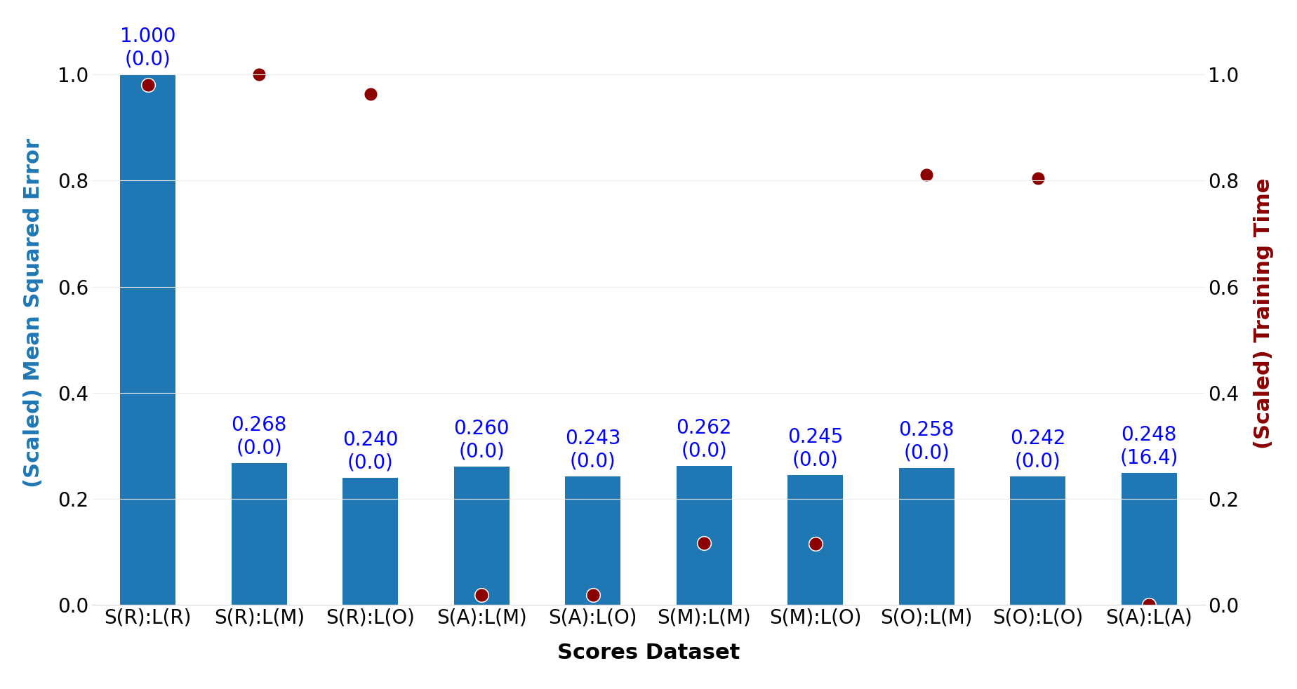
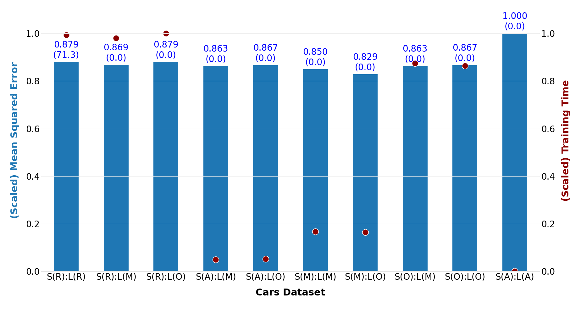
Figure 2: Performance evaluations on scores (left) and cars (right) datasets. The values on each bar represent the average MSE value and the average number of infeasible predictions (in paranthesis) on the test sets. The scatter plot shows the training time for each variant. Note that MSE and computation times are scaled according to the maximum value for the corresponding performance measure obtained by one of the variants.

In the cars dataset, the scikit-learn method S(A):L(A) exhibits the worst MSE score. Conversely, the variant that solves the optimization problem at the leaf node emerges as the top performer, underscoring the power of the proposed approach. Interestingly, we detect violations in the method employing relaxation in both split and leaf stages, which may be expected given that predictions derived from the relaxation do not guarantee feasibility, unlike other proposed methodologies.

As expected, the scatter plots show that the variants using relaxation or optimization for split evaluations take much longer time than those variants using the average or the medoid of the node. Taking into account the computation time, the MSE score, and particularly the feasibility, the variants that use optimization solely at the leaf nodes present an appealing compromise solution.

The comparison of the proposed variants for statistical significance is conducted using the Friedman test [9], and if a significant difference is detected by the Friedman test, it is followed by the Nemenyi test [17]. In Figure 3, we represent the test results applied to the cars and scores datsets. For the scores dataset, we observe that the $p$-value is practically 0, which indicates that the null hypothesis of identical variants can be rejected at the 0.95 confidence level. This means that there is a statistically significant difference in the performances of the variants with S(R):L(O) having a notably better performance when compared to the others. With the results for the cars dataset, we observe that the $p$-value for Friedman test is 0.226, signifying that the null hypothesis of identical variants cannot be rejected. Therefore, there is no statistically significant difference in the performances of the proposed variants.

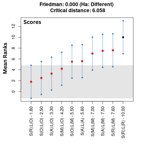
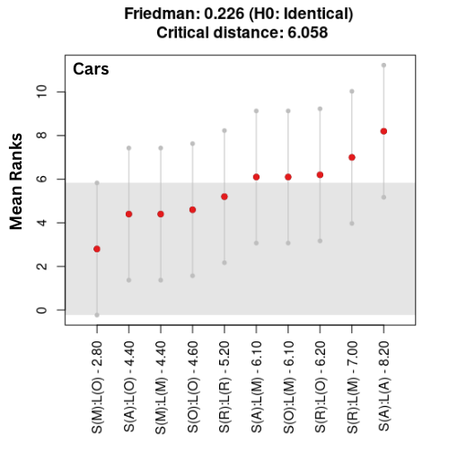
Figure 3: Friedman tests for measuring statistically significant differences on scores (left) and cars (right) datasets.

3.2 Synthetic Datasets

In this section, we use a synthetic dataset mimicking the motivating example of our introduction. This synthetic dataset encompasses multi-target regression data, providing us with a controlled environment for method evaluation. We call this dataset class and outline its generation process along with the underlying mathematical model in Appendix C.

In accordance with the experiments in Section 3.1, we utilize the same methodology with five-fold cross-validation. This is done to compare our nine variants using the same parameters. To leverage the advantage of synthetic generation, we evaluated our proposed variants across nine different datasets, varying in size and the number of targets. These datasets comprised combinations of 500, 1000, and 2000 rows, with total target values of 3, 5 and 7.

The MSE score and computation time are depicted in the left side of Figure 4, representing the average metrics across all nine datasets. On the right side of Figure 4, we see that $p$-value is close to 0, which indicates that the methods have statistically different performances at the 0.95 confidence level. We observe that none of the proposed algorithms produce infeasible predictions, unlike the scikit-learn method, S(A):L(A) which, despite yielding the lowest MSE among all approaches, generated the only positive average number of infeasible predictions. This suggests that the scikit-learn method compromised constraints to improve the predictions, a trade-off that is clearly not suitable for applications.

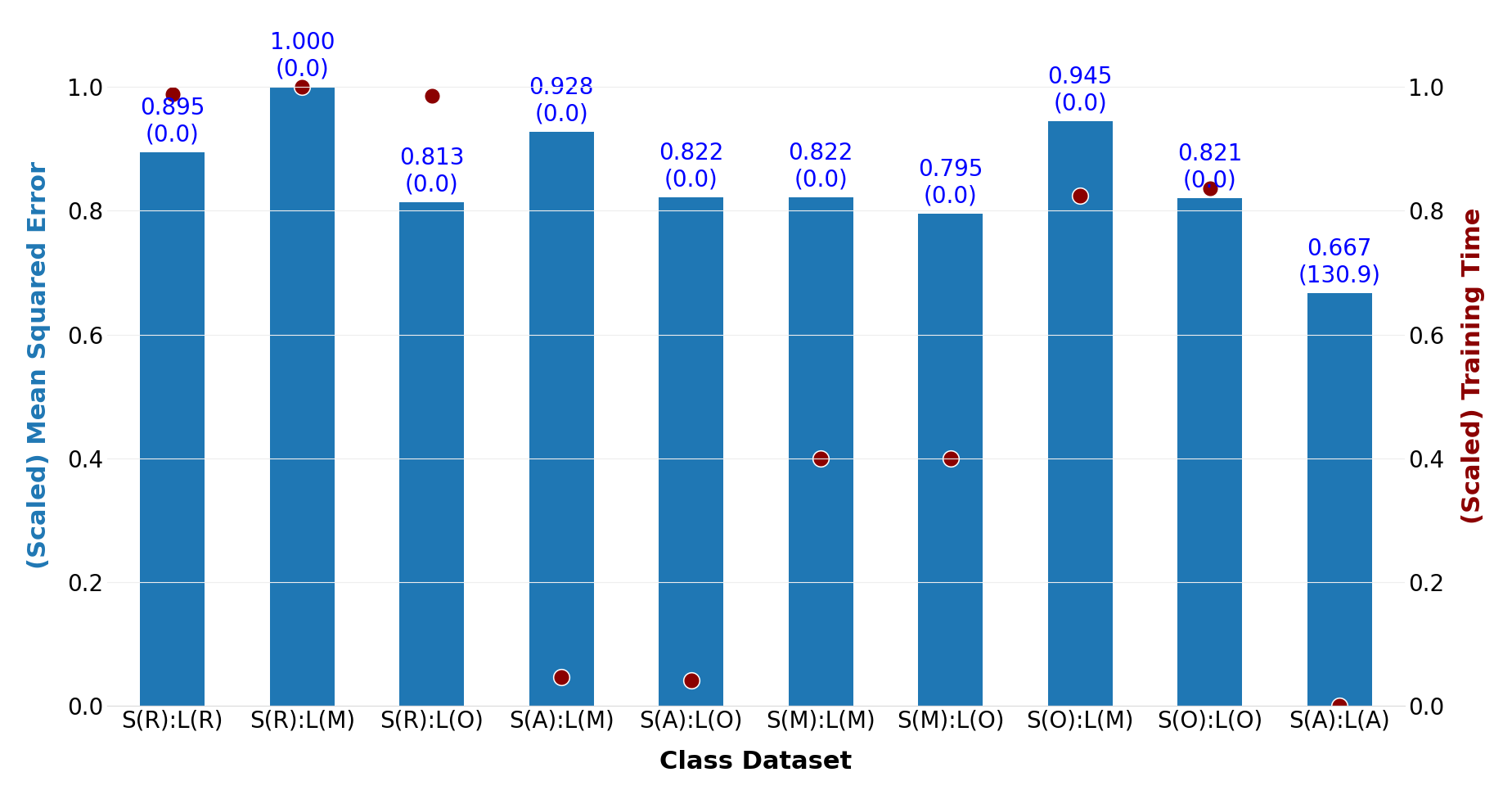
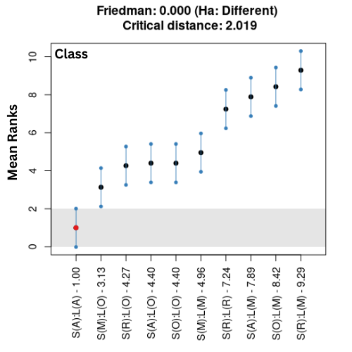
Figure 4: Performance metrics plot (left) and the Friedman test for statistical differences (right) on class datasets. The values on each bar of the left plot represent the average MSE value and the average number of infeasible predictions (in paranthesis) on the test sets. The scatter plot shows the training time for each variant. Note that MSE and computation times are scaled according to the maximum value for the corresponding performance measure obtained by one of the variants.

The boxplots in Figure 5 illustrate the MSE values and the duration times of all the variants across nine datasets with different sizes in terms of rows and targets. On the left side of the plot, the proposed variants show comparable MSE scrores. On the right side, the duration of the variants varies, with those involving optimization and relaxation displaying longer training times as before. Another noteworthy observation is that methods with relatively short training times tend to have higher MSE values.

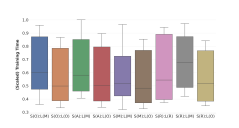
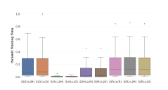
Figure 5: MSE (left) and training time (right) plots on synthetic class datasets.

Figure 6 illustrates a schematic representation of a tree trained on the class dataset. This tree structure is obtained by solving the optimization problem for the split evaluation as well for the leaf prediction; i.e., the selected variant is S(O):L(O). In this figure, the green nodes signify the leaf nodes, while the red nodes represent decision nodes where the data is split. Additionally, the splits after each decision node are depicted with arrows indicating the left and right child nodes, accompanied by text specifying the split feature and threshold. It is easy to observe on the tree plot that the OCDT made splits that are both accurate and feasible. As we outline in Appendix C, the target values are generated in a way that they are dependent on Grade and GradeAvgPrevElec. This is clearly depicted in the tree plot as the majority of splits employed by the OCDT used those features. Additionally, the second-level splits in the tree plot are dependent on the Class feature being one or higher, which aligns with the conditions imposing constraints to assign some targets to zero. This visualization example shows that OCDTs have the potential to be interpretable like their conventional counterparts available in machine learning packages.

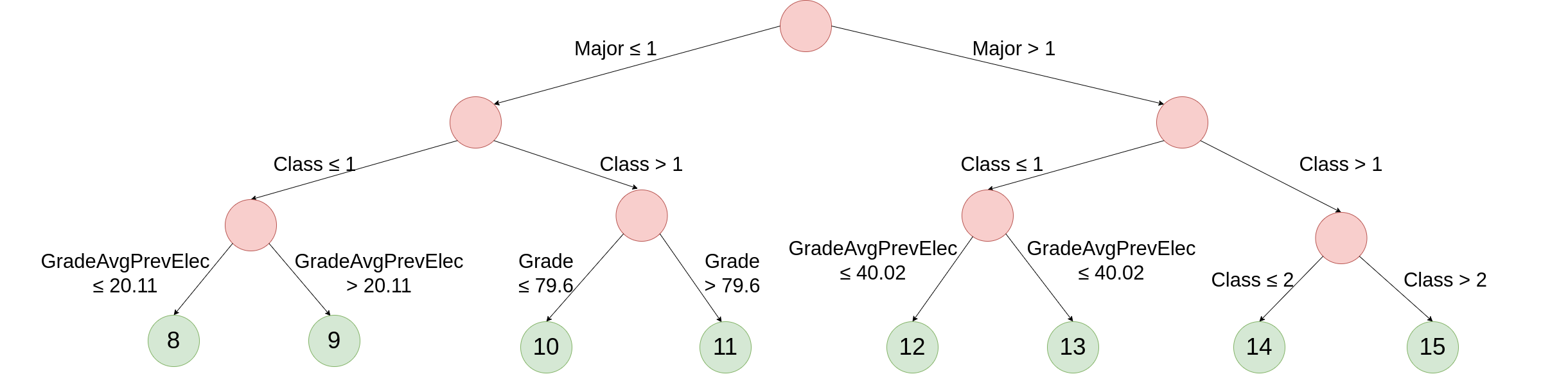
Figure 6: Visualization of an OCDT model on a sample class dataset.

As a result of our computational study, we conclude that the results underscore the effectiveness of the proposed approach, particularly in maintaining adherence to constraints while achieving competitive performance across diverse datasets. By integrating optimization in split evaluations and leaf predictions, our methodology demonstrates better predictive accuracy compared to traditional methods, even in datasets with complex constraints. These findings highlight the robustness and versatility of our approach, especially in scenarios where compliance to constraints among the targets is crucial.

4 Conclusion

We have introduced new methods to handle constraints among target variables in decision trees, an area yet unexplored in the existing literature. We have proposed an optimization-based exact approach and several heuristic approaches to ensure feasible predictions and maintaining computational efficiency. Through a computational study with existing and synthetic datasets, we have demonstrated the effectiveness of the proposed methods in producing feasible predictions, showcasing their potential for applications in multi-target learning.

Limitations.

The work presented here has a few limitations. Firstly, the optimization-based exact method can be computationally demanding for deep trees, which may impede its application for larger datasets. Secondly, the heuristic approaches proposed may not always produce accurate or even feasible predictions, limiting their reliability. Thirdly, when the constraints among targets are highly non-convex, solving the prediction problem at each node can prove challenging, potentially affecting the overall performance of the decision tree. Lastly, in its current form, it is unclear how these output-constrained decision trees can serve as the base learners for ensemble methods.

Future research.

We aim to investigate the integration of our approach into bagging methods like random forests, as trees often act as base learners in these methods. We are also interested in exploring a warm-start method in the exact approach, where an optimization problem needs solving at each node. Given that these nodes share a parent-child relationship, the subsets they create could aid in devising this method for subsequent problems at the child nodes once the parent node is resolved. We are also considering the inclusion of target constraints in optimization-based algorithms for training trees like, for example, optimal classification trees [3]. Although these algorithms can currently handle smaller problem sizes compared to standard implementations like CART [4], this is a promising research direction. Lastly, we are looking into the potential advantages of considering constraints in clustering, as training decision trees can be seen as a supervised clustering method.

Appendix A The Optimization Model of The scores Dataset

The optimization model imposed on the scores dataset is formulated as follows:

minimize $$\sum_{i=1}^{n}\sum_{j=1}^{k}(\hat{y}_{j}-y_{ij})^{2}$$

subject to $$\hat{y}_{j}\leq 110b_{j},\quad\quad j=1,\dots,k,\quad$$

$$\hat{y}_{2}\geq 50b_{3},\quad$$

$$\hat{y}_{1}+\hat{y}_{2}\geq 110b_{1},$$

where $n$ is the number of instances, $k$ is the number of targets, $\hat{y}_{j}$ is the prediction for the $j$-th target, $y_{ij}$ is the true value of the $j$-th target for the $i$-th instance, and $b_{j}$ is a binary variable indicating whether the prediction for the $j$-th target is used ($b_{j}=1$) or not ($b_{j}=0$).

Appendix B The Optimization Model of The cars Dataset

The optimization model imposed on the cars dataset is formulated as follows:

minimize $$\sum_{i=1}^{n}(\hat{y}_{1}-y_{i1})^{2}$$

subject to $$\hat{y}_{1}\geq b_{1},\quad$$

$$\hat{y}_{1}\leq Mb_{1},\quad$$

where $n$ is the number of instances, $\hat{y}_{1}$ is the prediction for the first target, $y_{i1}$ is the true value of the first target for the $i$-th instance, $b_{1}$ is a binary variable indicating whether the prediction for the first target is used ($b_{1}=1$) or not ($b_{1}=0$), and $M$ is a large constant representing the upper bound ($Mb_{1}$) on the prediction ($\hat{y}_{1}$) for the first target.

Appendix C Data Generation and The Optimization Model of The class Dataset

Table 1: Features of the class dataset

Features	Distribution	Min	Max	Mean	Std.Dev.
EnrolledElectiveBefore	Discrete Uniform	0	1	-	-
GradeAvgPrevElec	Normal	0	100	60	15
Grade	Normal	0	100	70	10
Major	Discrete Uniform	1	3	-	-
Class	Discrete Uniform	1	4	-	-
GradePerm	Normal	0	100	70	10

Table 1 outlines the distributions and their parameters used to generate the synthetic data, illustrating how the features of the dataset are created. We should note that the feature GradePerm consists of the permuted values of the feature Grade, created with the purpose of imposing randomness on the data. The target values are computed by taking the equally weighted sum of the Grade and GradeAvgPrevElec, with the addition of a uniform noise component ranging between -10 and 10 if GradeAvgPrevElec is non-zero. If GradeAvgPrevElec is zero, the target value is determined by Grade plus a normal noise with a mean of 10.0 and a standard deviation of 2.0. These computed values are then clipped to ensure they fall within the range of 0 to 100. Additionally, certain target values are deliberately set to zero based on random selection according to the features. For instance, if the Class feature is equal to one, all but a randomly chosen subset of the first two targets’ grades are set to zero. To fit the data to our research objectives, we have imposed two constraints on the created dataset. One constraint is created using binary decision variables to ensure that one non-zero prediction is generated at most. Another set of constraints has been applied to each target variable to limit the prediction based on the binary variable.

The optimization model is as follows:

minimize $$\sum_{i=1}^{n}\sum_{j=1}^{k}(\hat{y}_{j}-y_{ij})^{2}$$

subject to $$\sum_{j=1}^{k}b_{j}\leq 1,\quad$$

$$\hat{y}_{j}\leq 110b_{j},\quad$$

where $n$ is the number of instances, $k$ is the number of targets, $\hat{y}_{j}$ is the prediction for the $j$-th target, $y_{ij}$ is the true value of the $j$-th target for the $i$-th instance, and $b_{j}$ is a binary variable indicating whether the prediction for the $j$-th target is used ($b_{j}=1$) or not ($b_{j}=0$).

References

- Ben-David, [1995] Ben-David, A. (1995). Monotonicity maintenance in information-theoretic machine learning algorithms. Machine Learning, 19:29–43.
- Bertsekas, [1982] Bertsekas, D. (1982). Constrained Optimization and Lagrange Multiplier Methods. Computer Science and Applied Mathematics : A Series of Monographs and Textbooks. Academic Press.
- Bertsimas and Dunn, [2017] Bertsimas, D. and Dunn, J. (2017). Optimal classification trees. Machine Learning, 106(7):1039–1082.
- Breiman et al., [1984] Breiman, L., Friedman, J., Olshen, R., and Stone, C. (1984). Cart. Classification and Regression Trees.
- Calzavara et al., [2019] Calzavara, S., Lucchese, C., and Tolomei, G. (2019). Adversarial training of gradient-boosted decision trees. In Proceedings of the 28th ACM International Conference on Information and Knowledge Management, pages 2429–2432.
- Cardoso and Sousa, [2010] Cardoso, J. S. and Sousa, R. (2010). Classification models with global constraints for ordinal data. In 2010 Ninth International Conference on Machine Learning and Applications, pages 71–77. IEEE.
- Chen et al., [2019] Chen, H., Zhang, H., Boning, D., and Hsieh, C.-J. (2019). Robust decision trees against adversarial examples. In International Conference on Machine Learning, pages 1122–1131. PMLR.
- Chen and Zhang, [2020] Chen, Y. and Zhang, D. (2020). Physics-constrained deep learning of geomechanical logs. IEEE Transactions on Geoscience and Remote Sensing, 58(8):5932–5943.
- Friedman, [1940] Friedman, M. (1940). A comparison of alternative tests of significance for the problem of m rankings. The annals of mathematical statistics, 11(1):86–92.
- Gurobi Optimization, LLC, [2023] Gurobi Optimization, LLC (2023). Gurobi Optimizer Reference Manual. https://www.gurobi.com.
- Kaggle, [2018] Kaggle (2018). Car insurance claim data. https://www.kaggle.com/datasets/xiaomengsun/car-insurance-claim-data. Accessed on May 20, 2024.
- Kimmons, [2012] Kimmons, R. (2012). Exam Scores. http://roycekimmons.com/tools/generated_data/exams. Accessed on May 20, 2024.
- Lee and Kang, [1990] Lee, H. and Kang, I. S. (1990). Neural algorithm for solving differential equations. Journal of Computational Physics, 91(1):110–131.
- Lee et al., [2019] Lee, H., Lee, S. H., and Quek, T. Q. (2019). Constrained deep learning for wireless resource management. In ICC 2019-2019 IEEE International Conference on Communications (ICC), pages 1–6. IEEE.
- Lougee-Heimer, [2003] Lougee-Heimer, R. (2003). The common optimization interface for operations research: Promoting open-source software in the operations research community. IBM Journal of Research and Development, 47(1):57–66.
- Nanfack et al., [2022] Nanfack, G., Temple, P., and Frénay, B. (2022). Constraint enforcement on decision trees: A survey. ACM Computing Surveys (CSUR), 54(10s):1–36.
- Nemenyi, [1963] Nemenyi, P. B. (1963). Distribution-Free Multiple Comparisons. Princeton University.
- Pedregosa et al., [2011] Pedregosa, F., Varoquaux, G., Gramfort, A., Michel, V., Thirion, B., Grisel, O., Blondel, M., Prettenhofer, P., Weiss, R., Dubourg, V., Vanderplas, J., Passos, A., Cournapeau, D., Brucher, M., Perrot, M., and Duchesnay, E. (2011). Scikit-learn: Machine learning in Python. Journal of Machine Learning Research, 12:2825–2830.
- Raissi et al., [2019] Raissi, M., Perdikaris, P., and Karniadakis, G. E. (2019). Physics-informed neural networks: A deep learning framework for solving forward and inverse problems involving nonlinear partial differential equations. Journal of Computational Physics, 378:686–707.
- Rudin et al., [2022] Rudin, C., Chen, C., Chen, Z., Huang, H., Semenova, L., and Zhong, C. (2022). Interpretable machine learning: Fundamental principles and 10 grand challenges. Statistic Surveys, 16:1–85.
- Struyf and Džeroski, [2007] Struyf, J. and Džeroski, S. (2007). Clustering trees with instance level constraints. In Machine Learning: ECML 2007: 18th European Conference on Machine Learning, Warsaw, Poland, September 17-21, 2007. Proceedings 18, pages 359–370. Springer.
- Yan et al., [2022] Yan, B., Harp, D. R., Chen, B., and Pawar, R. (2022). A physics-constrained deep learning model for simulating multiphase flow in 3d heterogeneous porous media. Fuel, 313:122693.
- Zhang et al., [2022] Zhang, C., Zuo, R., Xiong, Y., Zhao, X., and Zhao, K. (2022). A geologically-constrained deep learning algorithm for recognizing geochemical anomalies. Computers and Geosciences, 162:105100.