Resource-Efficient Heartbeat Classification Using Multi-Feature Fusion and Bidirectional LSTM

Abstract

In this article, we present a resource-efficient approach for electrocardiogram (ECG) based heartbeat classification using multi-feature fusion and bidirectional long short-term memory (Bi-LSTM). The dataset comprises five original classes from the MIT-BIH Arrhythmia Database: Normal (N), Left Bundle Branch Block (LBBB), Right Bundle Branch Block (RBBB), Premature Ventricular Contraction (PVC), and Paced Beat (PB). Preprocessing methods including the discrete wavelet transform and dual moving average windows are used to reduce noise and artifacts in the raw ECG signal, and extract the main points (PQRST) of the ECG waveform. Multi-feature fusion is achieved by utilizing time intervals and the proposed under-the-curve areas, which are inherently robust against noise, as input features. Simulations demonstrated that incorporating under-the-curve area features improved the classification accuracy for the challenging RBBB and LBBB classes from 31.4% to 84.3% for RBBB, and from 69.6% to 87.0% for LBBB. Using a Bi-LSTM network, rather than a conventional LSTM network, resulted in higher accuracy (33.8% vs 21.8%) with a 28% reduction in required network parameters for the RBBB class. Multiple neural network models with varying parameter sizes, including tiny (84k), small (150k), medium (478k), and large (1.25M) models, are developed to achieve high accuracy across all classes, a more crucial and challenging goal than overall classification accuracy.

1 Introduction

Artificial Intelligence (AI) is revolutionizing healthcare, driven by advancements in high-performance computing systems, the availability of massive datasets, and the progress of efficient deep neural networks (DNNs). Deep learning is widely used in a variety of medical applications, including the processing of medical images via convolutional neural networks (CNNs), feature extraction from physiological signals sampled as time-series data using recurrent neural networks (RNNs), and the processing of electronic health records (EHRs) [1]. Cardiovascular disease (CVD) remains the leading cause of death globally, with deaths rising from 12.1 million in 1990 to 20.5 million in 2021, according to the World Heart Federation (WHF) [2]. The electrocardiogram (ECG) is the most commonly utilized physiological signal for detecting CVDs [3]. Recently, deep learning has shown promising results in the processing and classification of ECG signals for CVD diagnosis [4, 5, 6, 7, 8, 9, 10, 11, 12, 13]. Resource-efficient ECG classification can help to develop affordable wearable medical devices, making them accessible to populations across various income levels, and providing significant societal and economic impacts [14, 15].

Recent research extensively leverages deep learning models [16] to decipher intricate patterns in ECG data and achieve higher classification accuracy. In [17], arrhythmia classification across 12 classes of ECG data, recorded from 53,549 patients, achieved an F1 score of 84% using a deep CNN with 43 million parameters. Using a CNN with 153k parameters, [8] achieved an accuracy of 93.6% for arrhythmia classification within the MIT-BIH dataset. [18] reached a 94% accuracy on AAMI classes using a CNN with 20k parameters. [5] employed a deep residual CNN with 99k parameters and achieved 93% accuracy on AAMI classes [19]. In contrast, [12] developed a CNN with 197k parameters but achieved a lower accuracy of 92% on the AAMI classes. The highest classification accuracy of 99.90% on AAMI classes was achieved by [13] using a large model with 4 million parameters. However, most of these models demand high computational power, making them challenging to implement for real-time classification on resource-constrained wearable devices [20, 21]. In an innovative approach, [11] co-designed a lightweight CNN with analog computing circuits, achieving 95% accuracy on AAMI classes with only 336 parameters Recurrent neural networks (RNNs) offer a promising avenue to enhance ECG classification. RNNs can concurrently leverage spatial and temporal features extracted from ECG data to improve accuracy and reduce the size of the network. [10] proposed a hybrid CNN-LSTM model with 64k parameters and achieved an accuracy of 98.2%. Similarly, [9] developed a hybrid CNN-LSTM model achieving an accuracy of 97.87%. A common problem in many of these works is the reliance on overall accuracy as the main performance metric, while it is essential to ensure high accuracy across all classes. Some of these classes may indicate critical cardiovascular conditions, and their accurate detection can potentially save lives.

The main contributions of this work are as follows:
1. Utilizing original heartbeat data annotations from the MIT-BIH Arrhythmia Database [22], five classes are selected, and a design strategy is applied to develop neural networks that achieve high classification accuracy across all classes. The use of original heartbeat classes, unlike some other works which have constructed mixed classes, leads to more clinically relevant results.
2. A multi-feature fusion approach is proposed to combine the time interval and the proposed under-the-curve area features extracted from the ECG signal, enhancing accuracy and robustness. Simulations demonstrate that by including the area features, accuracy for the challenging RBBB and LBBB classes significantly improves from 31.4% to 84.3% for the RBBB class, and from 69.6% to 87.0% for the LBBB class.
3. A bidirectional LSTM (Bi-LSTM) network is used for classification, achieving higher accuracy compared to the conventional LSTM network. Simulations presented in the paper indicate that the Bi-LSTM network provides substantially higher accuracy (33.8% versus 21.8%) for the RBBB class while requiring 28% fewer parameters.
4. A resource-efficient classification approach is adopted which, unlike most works optimized solely for the maximum accuracy, results in small er networks with descent accuracy. Four neural networks with varying parameter sizes, including tiny (84k), small (150k), medium (478k), and large (1.25M) models, are developed and benchmarked against state-of-the-art.

2 Approach

2.1 Dataset

The MIT-BIH Arrhythmia Database [22] consists of 48 ECG records, each 30 minutes in duration, sampled at a rate of 360 Hz. In this work, the database records are partitioned as two-thirds for training and one-third for testing. We extracted the number of different arrhythmia types in the dataset, as shown in Fig. 1. The normal heartbeat (N) and the four most common arrhythmia heartbeats, Right Bundle Branch Block (RBBB), Left Bundle Branch Block (LBBB), Premature Ventricular Contraction (PVC), and Paced Beat (PB), are selected for classification. In future work, including more classes can provide more clinically relevant results, but this will necessitate the use of a more complex neural network, which complicates resource-efficient implementation. RBBB, while benign in healthy subjects, has been associated with an increased risk of heart failure and atrial fibrillation in patients. LBBB, less common in healthy individuals than RBBB, typically indicates underlying cardiac issues and is linked with a higher risk of serious cardiac events such as heart failure and sudden cardiac death in CVD patients [23]. Consequently, detecting these classes accurately is of vital importance. However, many previous works have combined these two classes with the normal class. PVC is generally benign in healthy individuals but can signal an increased risk of cardiac death in CVD patients. PB is typically observed in patients with an active pacemaker. We use the MIT-BIH standard as it can provide more accurate medical information compared to the AAMI standard [19]. In the AAMI standard, heartbeats are labeled into four main classes: Normal (N), Supraventricular Ectopic Beat (SVEB), Ventricular Ectopic Beat (VEB), and Fusion (F) [19]. The normal class comprises the MIT-BIH classes N, RBBB, and LBBB. However, the significant risks associated with RBBB and LBBB indicate that this can overlook critical medical conditions.

Figure 1: Distribution of data annotations in the MIT-BIH Arrhythmia Database.

2.2 Preprocessing

The recorded ECG signal is often distorted by noise and artifacts, which can hinder the extraction of key morphological features in the ECG waveform. Specifically, features with lower signal power, such as the P peak and Q dip, can be significantly affected by noise. Therefore, it is essential to mitigate this noise through preprocessing. The spectrum of noise and distortion signals is time-dependent, rendering conventional Fourier transform approaches ineffective for filtering. Instead, the discrete wavelet transform (DWT) can be used to suppress noise and distortion signals. The approach presented in [24, 25] is used to suppress noise. The Daubechies 4 (DB4) wavelet, which closely resembles the ECG signal waveform, is utilized in this work. This wavelet features a normalized central frequency $k_{c}\approx 0.7$. The pseudo-frequency for scale $n$ is calculated as $f_{n}=k_{c}f_{s}/2^{n}$, where $f_{s}$ is the sampling frequency of the ECG signal (360 Hz) [25]. The low-frequency noise, primarily baseline drift, is mostly concentrated around 0.5 Hz. Therefore, to achieve $f_{n}\leq 0.5$ Hz, the signal decomposition should be performed up to the scale 9. Spectrum of the ECG signal spans a bandwidth of 0.05–100 Hz. However, most of the signal power lies within the 8–20 Hz band. It has been demonstrated that decomposition up to level 6 is necessary to capture this frequency band effectively [24]. High-frequency noise, often due to random body movements, usually is spread at frequencies above 50 Hz [25]. This noise is attenuated by discarding the detailed coefficients of levels 1, 2, and 3. Therefore, the signal is reconstructed using the detailed coefficients of levels 4, 5, and 6, along with the approximate coefficient of level 9. The raw and filtered ECG signals are shown in Fig. A.1 (Appendix A.1).

2.3 Multi-Feature Fusion

Multi-feature fusion involves combining various types of data or features from multiple sources or modalities to enhance classification accuracy. Features can encompass diverse forms such as images, text, audio, video, or different metrics extracted from the same dataset. In this paper, we extract two sets of features from the dataset, time intervals $T_{ij}$ and under-the-curve areas $A_{ij}$, from main points (PQRST) in the ECG signal waveform. These two sets, comprising six time intervals and four under-the-curve areas, are integrated using an early fusion approach, and the combined results are fed into the classification pipeline.

The extracted time intervals include $T_{\rm RR}$, $T_{\rm PR}$, $T_{\rm RT}$, $T_{\rm QR}$, $T_{\rm RS}$, and $T_{\rm PT}$. The RR interval is defined as the time difference between the T peaks of consecutive heartbeats. The other time intervals, $T_{ij}$, are defined as the time differences between two main points within a single heartbeat, where $T_{ij}=t_{j}-t_{i}$. The extracted under-the-curve areas include $A_{\rm PQ}$, $A_{\rm ST}$, $A_{\rm QR}$, and $A_{\rm RS}$. These features are calculated as the sum of the absolute values of the signal samples located between two main points, inclusive of the points themselves, expressed as $A_{ij}=\sum_{k}{|x(t_{k})|}$. An important advantage of the under-the-curve area features is their robustness against noise, as a result of the inherent averaging property of the summation function.

2.4 Detection of Main Points in ECG Signal

For each of the main points (PQRST) in the ECG signal waveform, a specific algorithm should be employed to achieve high accuracy. The MIT-BIH dataset provides standard annotations for only the R and P peaks, which facilitates the evaluation of their detection accuracy. However, for the other main points, accuracy estimation is not possible. The effectiveness of these detection algorithms can ultimately be validated through the overall accuracy of the heartbeat classification (Section 3).

2.4.1 Detection of R Peaks

In this work, two moving average windows are employed to implement adaptive blocks for the accurate detection of the R peaks:

$$y_{p}[n]=\frac{1}{2N+1}\sum_{k=-N}^{N}x[n+k]$$ (1)

$$y_{w}[n]=\frac{1}{2M+1}\sum_{k=-M}^{M}x[n+k].$$ (2)

The first moving average (peak) $y_{p}[n]$ is used to identify the QRS complex and the second moving average (window) $y_{w}[n]$ serves as a threshold for the first. It is important that the length of the first window, $N$, is shorter than that of the second window, $M$, to maintain effective detection. Specifically, the first window’s length is set at 36 samples (100 ms), corresponding to the duration of a typical QRS complex. A threshold of 0.3 is applied to this window to exclude noise that could mistakenly be identified as the QRS complex. The length of the second window is determined by the typical duration of a normal heartbeat, set at 120 samples (330 ms). A Block of Interest (BOI) is defined such that it equals 1 when $y_{p}[n]>y_{w}[n]$ and 0 otherwise. This function generates a sequence of rectangular pulses with adaptive widths, which are then used to detect the R peaks. In Fig. A.2 (Appendix A.1), samples of the ECG signal, peak and wave moving averages, and BOI are shown. This approach resulted in the sensitivity and precision higher than 90% across the records.

2.4.2 Detection of P and T Peaks

To detect the P and T peaks, a similar approach using dual moving average windows is employed, as with the R peak detection. The significantly higher amplitude of R peaks compared to the P and T peaks presents a detection challenge. To address this, the QRS complex is removed from the signal by zeroing a specific number of samples both before and after each R peak. Specifically, 30 samples preceding and 60 samples following the R peak are set to zero, based on the typical duration of the QRS complex in a normal heartbeat. The ECG signal with annotated P peaks and the signal after removing the QRS complex are shown in Fig. A.3 (Appendix A.1). Next, the dual moving averages method is applied to the signal with the QRS complex removed, which allows for the detection of both P and T peaks. However, these peaks must be distinguished using additional processing. The length of the peak moving average is determined based on the duration of the P wave in a normal heartbeat, which is 20 samples (55 ms). Similarly, the length of the wave moving average is set according to the normal QT interval at 40 samples (110 ms). To distinguish between the P and T peaks, the method calculates the distance from the maximum point of each detected peak to the nearest R peak [24]. For P peaks, the distance to the closest R peak, $T_{\rm PR}$, ranges from 20 to 170 samples (55 to 470 ms). For T peaks, the distance to the R peak is between 40 and 210 samples (110 to 583 ms). Peaks are classified as either P or T based on these criteria. This method, allowing an error tolerance of 36 samples (100 ms), achieved a sensitivity of 84.6% for detecting P peaks. However, the accuracy for T peaks could not be assessed due to the absence of reference annotations.

2.4.3 Detection of Q and S Dips

The Q and S dips in the ECG signal waveform are detected using a similar dual moving averages approach. Unlike the P and T peaks, the QRS complex is retained in the signal. The detected R peaks serve as reference points for identifying the Q and S dips. These two dips are located on either side of the R peak at varying distances, which facilitates their detection. For the Q point, the maximum distance from the R peak, $T_{\rm QR}$, is 20 samples (55 ms). Similarly, for the S point, the maximum distance from the R peak, $T_{\rm RS}$, is 40 samples (110 ms).

2.4.4 Detection Results

A sample of the detected main points on the ECG signal is shown in Fig. 2. The MIT-BIH database provides standard annotations only for the R and P peaks. Therefore, we can assess the accuracy of detected R and P peaks by using these standard annotations as references. The sensitivity and precision for the R peaks are very high at 99.8% and 99.95%, respectively. For the P peaks, these metrics are recorded at 84.0% and 84.6%, respectively. However, the detection accuracy of other main points cannot be evaluated due to the absence of reference annotations in the MIT-BIH database.

Figure 2: Sample of detected main points (PQRST) in the ECG signal.

2.5 Classification

2.5.1 Classification Approach

The two sets of extracted features, time intervals and under-the-curve areas, are integrated using an early fusion strategy. The combined results are then fed into the classification pipeline. A major challenge in this classification process is the imbalanced size of the classes, especially the normal (N) heartbeat class (see Fig. 1). Most previous works report overall accuracy as the main performance metric for classifiers [5, 26]. However, this approach can mask the lower accuracy in smaller, more challenging classes, such as RBBB and LBBB. From a medical diagnostic perspective, accurately classifying these arrhythmic classes is crucial. Therefore, we have focused on an approach that ensure high classification accuracy across all classes. We evaluate LSTM and Bi-LSTM-based neural networks in terms of classification accuracy and model size.

2.5.2 LSTM Networks

In the preliminary simulations discussed in this subsection, we exclusively used the six time interval features ($T_{ij}$) to provide deeper insights. All models were implemented, trained, and tested using Python. We employed the sparse categorical cross-entropy loss function in the algorithms, as detailed in Appendix A.2. The network architecture, depicted in Fig. 3(a), includes two LSTM layers, two dense layers, and a dropout layer [27]. We investigated various networks built using this configuration, adjusting the number of units, $n_{1}$ and $n_{2}$, in the two LSTM layers, as well as the dropout rate, $p$. The classification results for three scenarios are presented in Figs. 3(b)-(d).

We have intentionally not reported the overall accuracy to emphasize the accuracy of individual classes. The overall accuracy, typically dominated by the N class, which is the easiest to classify, can mask the inaccuracies in other classes. As expected, the N class achieves high accuracy, while the RBBB and LBBB classes present the greatest challenges for precise classification. For instance, Fig. 3(b) reveals a low accuracy of 21.81% for the RBBB class in the confusion matrix. Here, the precision metric is significantly higher than the recall metric (71.55% vs 26.22%), resulting in an F1 score of 38.37%. In an initial effort to improve accuracy, we doubled the number of LSTM units, with results displayed in Fig. 3(c). This modification remarkably improved the accuracy for the RBBB class (the accuracy of 58.48% and the F1 score of 60.25%), though the accuracy and F1 scores for the LBBB and PVC classes showed only minor improvements. This suggests that a substantial increase in the number of LSTM units is necessary to significantly improve accuracy for these classes. However, such an approach results in a larger model, which conflicts with our goal of resource-efficient implementation. By reducing the dropout rate from 0.5 to 0.25, as shown in Fig. 3(d), the model achieves higher accuracy across all classes, especially for the RBBB class, with an accuracy of 46.10% and an F1 score of 57.03%.

Figure 3: (a) Neural network architecture using LSTM layers and the six time interval features, (b) classification results for $n_{1}=n_{2}=64$ and $p=0.5$, (c) classification results for $n_{1}=n_{2}=128$ and $p=0.5$, (d) classification results for $n_{1}=n_{2}=64$ and $p=0.25$.

2.5.3 Bi-LSTM Networks

Intuitively, in a sequence of human heartbeats, each signal is correlated with its preceding and succeeding heartbeats. Thus, a Bi-LSTM network, which computes neuron outputs using both past (backward) and future (forward) states [28], has the potential to achieve higher accuracy. However, training Bi-LSTM networks can be challenging due to the presence of dual signal flow paths. Fig. 4(a) illustrates the architecture of the classification network, which comprises Bi-LSTM, dense, and dropout layers. This network maintains the same architecture as that shown in Fig. 3(a), with the exception that LSTM layers are replaced by Bi-LSTM layers to facilitate a fair comparison. Additionally, only the six time interval features are used as inputs to the network. Classification results for three representative networks are depicted in Fig. 4. Specifically, Fig. 4(b) shows the results for a network including Bi-LSTM layers with $n_{1}=n_{2}=32$ units each, and a dropout layer with a 0.5 dropout rate. The number of units in the Bi-LSTM network is set at half that of the LSTM network to ensure both networks have approximately the same number of parameters. Consequently, this Bi-LSTM-based network comprises about 42.5k parameters, compared to a similar LSTM-based network with 64 units which comprises about 58.9k parameters. A comparison between Fig. 4(b) and Fig. 3(b) reveals that the Bi-LSTM network achieves significantly higher accuracy (33.79% vs 21.81%) and F1 score (43.09% vs 38.37%) for the RBBB class, while reducing the number of parameters by 28%. This demonstrates a promising avenue for resource-efficient realization of the classification network.

Figure 4: (a) Neural network architecture using Bi-LSTM layers and the six time interval features, (b) classification results for $n_{1}=n_{2}=32$ and $p=0.5$, (c) classification results for $n_{1}=n_{2}=64$ and $p=0.5$, (d) classification results for $n_{1}=n_{2}=32$ and $p=0.25$.

2.6 Impact of Multi-Feature Fusion

In this section, we explore the impact of multi-feature fusion on the performance of the classification network. The confusion matrices for three scenarios of input features are shown in Fig. 5. The network architecture remains consistent with that depicted in Fig. 4(a), featuring two 64-unit Bi-LSTM layers and a dropout rate of 0.5. It is concluded that by incorporating two area features along with the six time intervals, the accuracy for the RBBB class significantly increases from 31.40% to 68.27%. Similarly, the accuracy for the LBBB class improves from 69.58% to 86.01%. With the comprehensive multi-feature fusion, that is, combining six time intervals and four area features, the accuracy for the RBBB class reaches 84.30%. Furthermore, the accuracy for all other classes also shows improvement over using only time interval features.

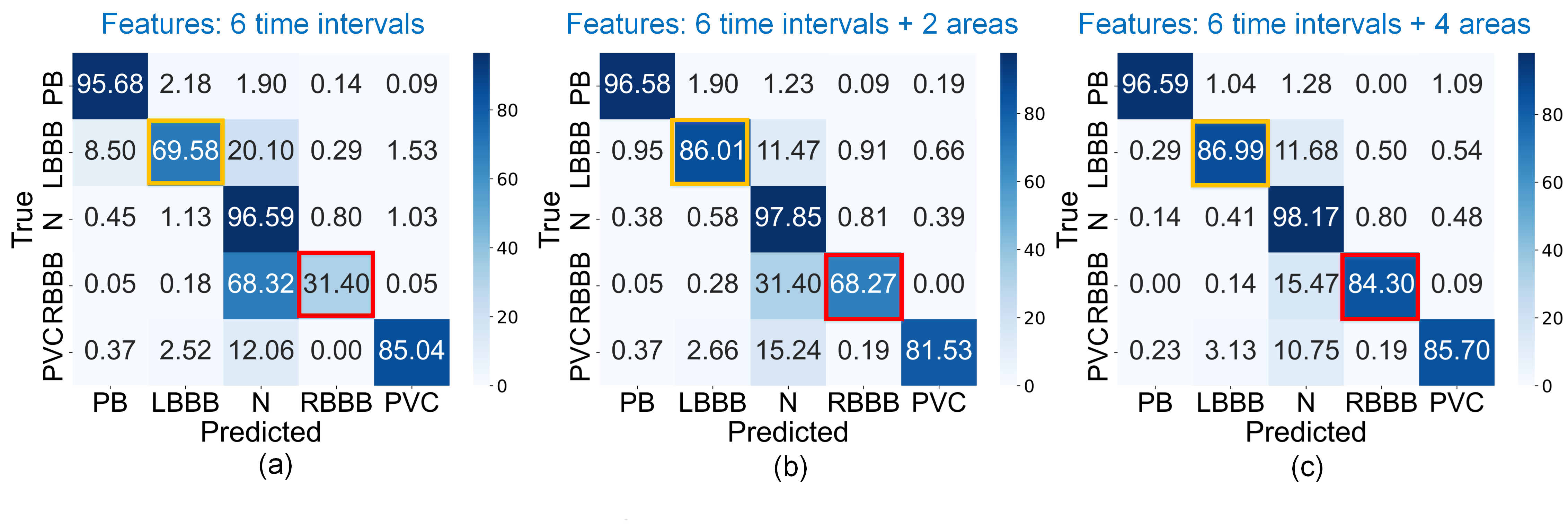
Figure 5: Classification results for the Bi-LSTM based network with different input features. (a) six time interval features, (b) six time intervals + two area features, (c) six time intervals + 4 area features.

3 Experiments

Leveraging the insights from preliminary investigations, we developed and evaluated several models to achieve high accuracy across all classes while maintaining a small model size for resource-efficient implementation. These models are realized using multiple Bi-LSTM layers, with the number of units in each layer scaled to achieve optimal accuracy. The architecture of the four developed models is illustrated in Fig. 6(a). All networks apply a multi-feature fusion strategy, incorporating six time intervals and four under-the-curve areas. The networks are trained using the mini-batch gradient descent method. Further details are provided in Appendix A.2. To prevent model overfitting, training and test losses were monitored across epochs (Appendix A.2).

Figure 6: Neural network architecture, accuracy, the number of parameters, the number of FLOPs, and the F1 score of each heartbeat class for the four developed models.

Four models of varying sizes are presented as representatives of the developed models: a tiny model (T) with 84k parameters, a small model (S) with 150k parameters, a medium model (M) with 478k parameters, and a large model (L) with 1.25M parameters. The performance of these models is summarized in Table 1. Fig. 6 compares the neural network architecture, overall accuracy, number of parameters, memory, number of FLOPs, and the F1 score for each heartbeat class across the four models. Notably, there are only slight variations in overall accuracy between models of significantly different sizes. The F1 score for class N is nearly consistent across all models and closely follows the overall accuracy as shown in Fig. 6. For the challenging RBBB class, the best F1 score is achieved with the large model, while the tiny model exhibits the lowest F1 score.

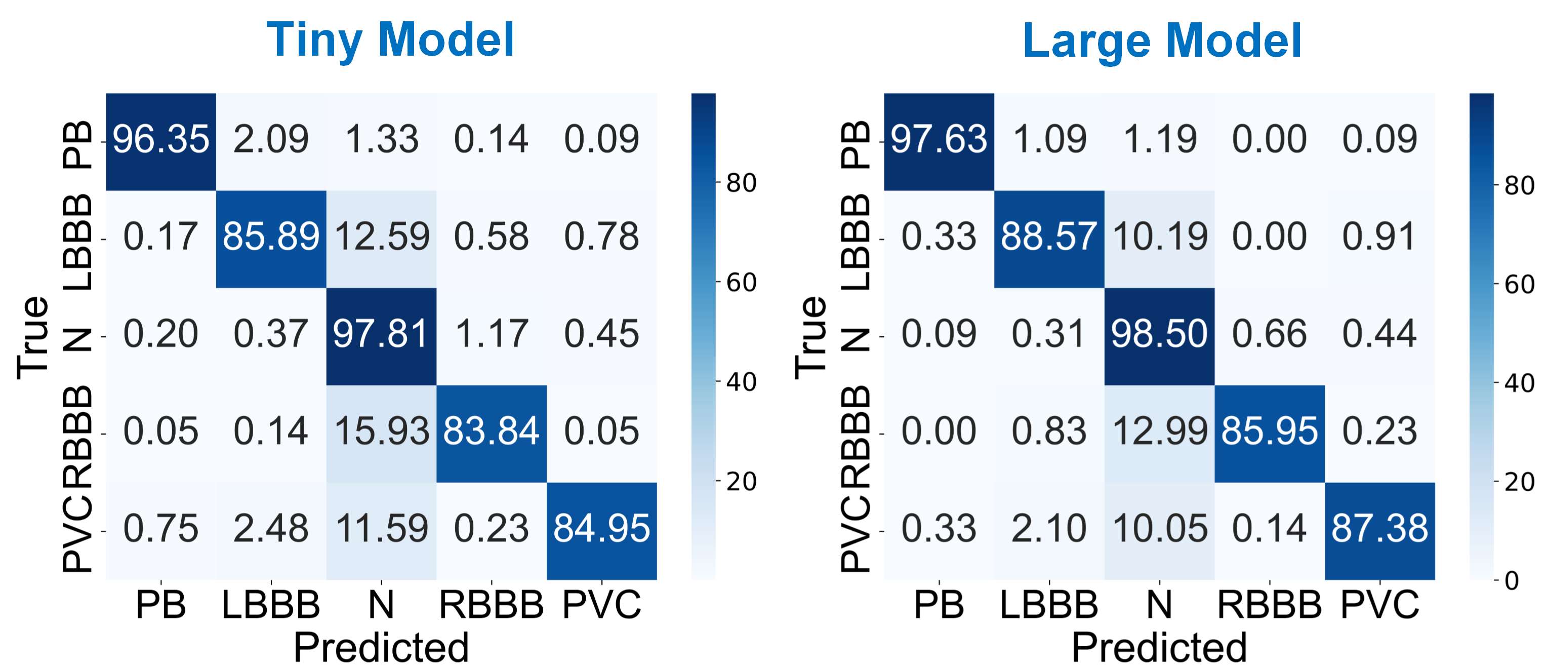
Figure 7: Confusion matrix for the developed tiny (T) and large (L) models.

Confusion matrices for the tiny (T) and large (L) models are shown in Fig. 7. The matrices are predominantly diagonal with small non-diagonal elements, indicating that both models are effective in distinguishing between the classes. To further illustrate this, t-SNE visualizations [29] for the two models are shown in Fig. 8. The models have effectively clustered most of the data samples, with only minor exceptions in the tiny model and a few points in the large model. The challenges of developing these models for dataset classification are evident in the t-SNE plots, such as, the large size of the N class and the close proximity of the difficult RBBB class to the N class. The two t-SNE plots also indicate high capabilities of the large model to effectively separate the heartbeat classes, which was not clear from the accuracy and F1 score metrics.

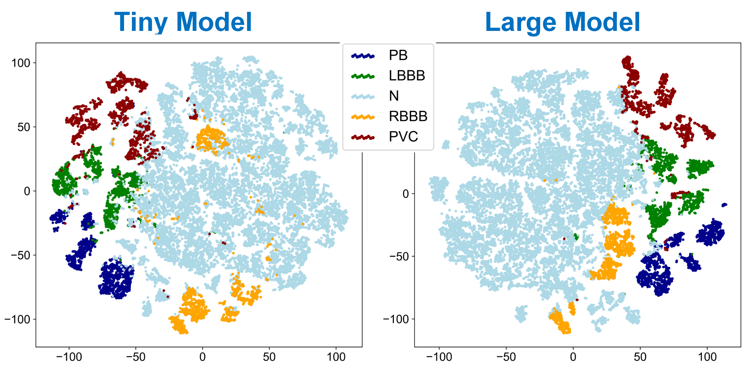
Figure 8: t-SNE visualization for the developed tiny (T) and large (L) models.

Table 1: Performance summary of the four developed models.

		F1 Score (%)
Model	Acc (%)	N	PB	LBBB	RBBB	PVC	Param	Memory	FLOPs
Tiny	94.7	96.9	96.6	88.8	85.1	89.1	83973	328 kB	71584
Small	95.1	97.2	97.2	89.4	87.2	89	149765	585 kB	121472
Medium	95.5	97.1	97.6	91.4	84.8	89.6	478469	1.83 MB	351872
Large	96.1	97.6	98	90.8	89.1	90.4	1250053	4.77 MB	996992

In Table 2, we compare the performance of our developed tiny (T) and large (L) models with state-of-the-art heartbeat classification models. The feature fusion and Bi-LSTM-based neural networks implemented in this work have resulted in higher accuracy and more compact networks. We utilized the original annotations available in the MIT-BIH database. In the literature, heartbeat classes are often defined based on varying criteria, making fair comparisons with these works challenging. For instance, [5] defines the class N as encompassing the N, RBBB, LBBB, AEB, and NEB annotations from the MIT-BIH dataset (Fig. 1). However, as we discussed earlier, it is crucial to separate these classes. In Table 2, the F1 score for each heartbeat class is provided for a rough comparison of the models. This metric is more practically useful than the overall accuracy, which many works have used as the primary measure of performance.

Table 2: Comparison of the developed tiny (T) and large (L) models with state-of-the-art.

				F1 Score (%)
Ref	Features	Classifier	Acc (%)	N	PB	LBBB	RBBB	PVC	Param
[5]	ECG beats	Res CNN	93.4	90.9	—	—	—	92.5	99k
[30]	Raw ECG, $T_{\rm RR}$	ESN	97.9	overall F1 score: 89.7%					30k
[25]	$T_{\rm PR}$, $T_{\rm RT}$, age, sex	SVM	82.2	68.4	100	13.0	100	100	—
[25]	$T_{\rm PR}$, $T_{\rm RT}$, age, sex	MLP	80.0	77.9	85.1	76.5	74.8	91.6	—
[7]	PCA	LSTM	93.5	overall F1 score: 91.7%					—
[8]	Raw ECG	CNN	93.6	———-					153k
[9]	Raw ECG	CNN-LSTM	97.8	98.4	—	—	—	—	—
[10]	Raw ECG	CNN	97.4	—	—	95.0	96.9	—	727k
[10]	Raw ECG	LSTM	97.1	—	—	94.8	96.4	—	52k
[10]	Raw ECG	CNN-LSTM	98.2	—	—	97.0	97.9	—	64k
Model T	6 $T_{ij}$, 4 $A_{ij}$	Bi-LSTM	94.7	96.9	96.6	88.8	85.1	89.1	84k
Model L	6 $T_{ij}$, 4 $A_{ij}$	Bi-LSTM	96.1	97.6	98.0	90.8	89.1	90.4	1.25M

4 Conclusion

In this paper, we presented a resource-efficient approach for the classification of heartbeat data from the MIT-BIH Arrhythmia Database. To enhance the quality of the raw ECG signal, preprocessing was performed using discrete wavelet transform and dual moving averages. We proposed a multi-feature fusion strategy to extract time intervals and under-the-curve areas from the ECG signal, demonstrating that this fusion significantly improves the accuracy of heartbeat classification. The classifier neural networks were implemented with bidirectional LSTM (Bi-LSTM), dense, and dropout layers in four different sizes. Their performance was extensively evaluated and compared with state-of-the-art models.

Appendix A Appendix

A.1 Preprocessing Results

Fig. A.1 shows the raw ECG signal and reconstructed signal after filtering the low- and high-frequency noise. The filtered signal has clean main points (PQRST), which is important for an accurate feature extraction. In Fig. A.2, the ECG signal (filtered), the peak moving average $y_{p}[n]$ defined in (1), the wave moving average $y_{w}[n]$ defined in (2), and the block of interest (BOI) for detection of R peaks is shown. ECG signal with annotated P peaks and the signal after removing the QRS complex are shown in Fig. A.3.

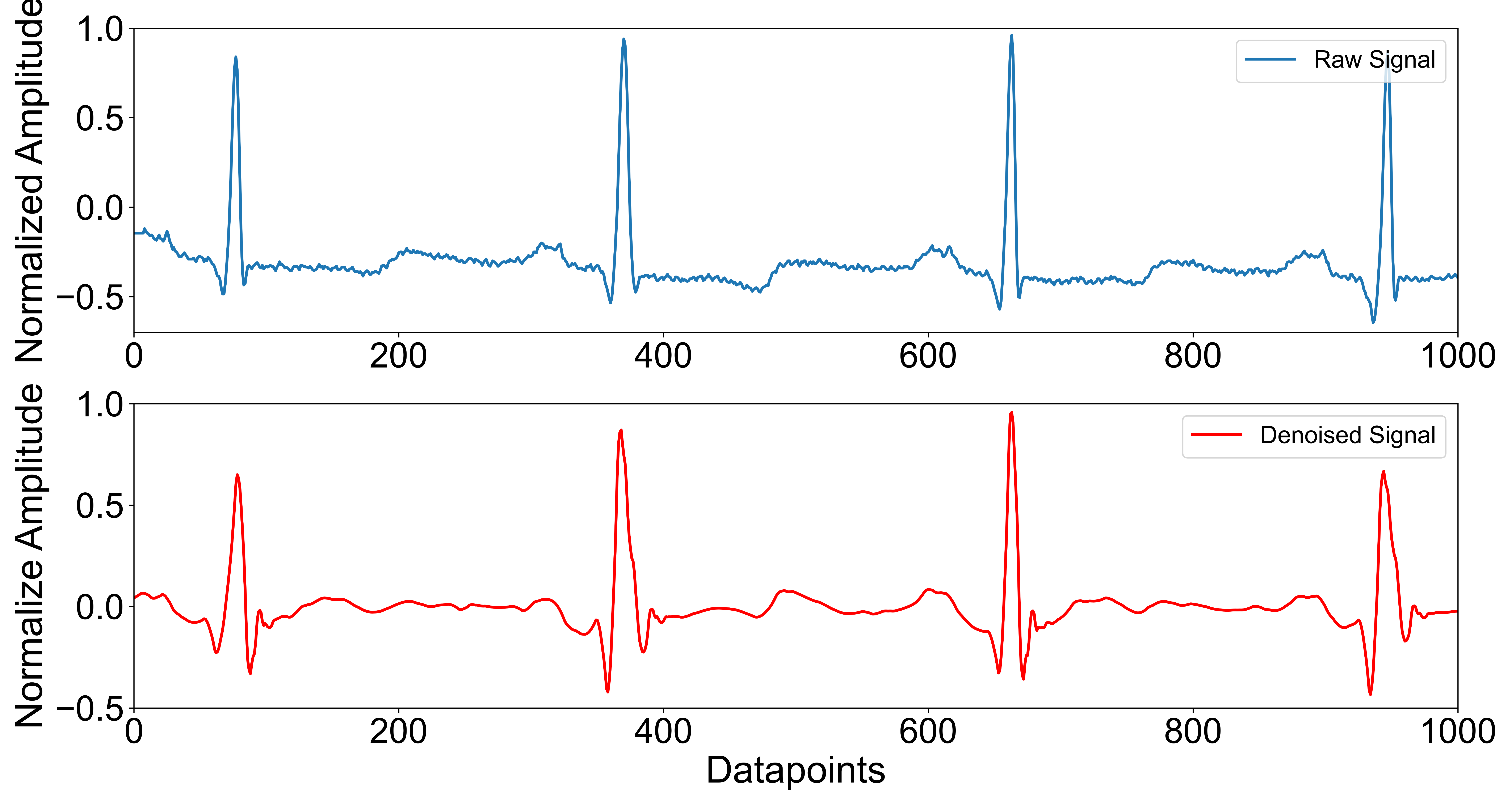
Figure A.1: The raw and reconstructed filtered ECG signal waveforms.

Figure A.2: ECG signal, peak and wave moving averages, and block of interest (BOI) for detection of R peaks.

Figure A.3: ECG signal with annotated P peaks and the signal after removing the QRS complex.

A.2 Training and Test Losses

In all of the LSTM and Bi-LSTM layers, the tanh activation function is used. Activation function used in the first dense layer is ReLU and in the second dense laser, the softmax function is used. The four developed models are trained using mini-batch gradient descent with a batch size of 64. The number of training samples is 73180. Each epoch takes 1143 iterations. The sparse categorical cross-entropy loss function defined as $L=-\frac{1}{N}\sum_{i}\log(p_{i})$ is used in the models. Loss is computed using the TensorFlow package in Python. In Fig. A.4, training and test losses are shown for the four models. All models are trained up to an epoch number of 10, which roughly provides a good compromise between training and test loss without overfitting.

Figure A.4: Training and test losses of the developed four models.

A.3 Computational Resources

The neural networks presented in the paper were trained and evaluated on a laptop with Intel64 Family 6 Model 142 Stepping 9 Genuine-Intel 2511 MHz CPU and 8 GB RAM. The number of parameters in the models are as follows. Tiny (T) model: 83973 parameters, small (S) model: 149765 parameters, medium (M) model: 478469 parameters, and large (L) model: 1250053 parameters. Memory size of the models is 328 kB for T model, 585 kB for S model, 1.83 MB for M model, and 4.77 MB for L model. Training time of the models is about 9, 12, 29, and 67 minutes, and their runtime is 13, 14, 23, and 86 ms/beat, for the T, S, M, and L models, respectively.

References

- [1] A. Esteva, A. Robicquet, B. Ramsundar, V. Kuleshov, M. DePristo, K. Chou, C. Cui, G. Corrado, S. Thrun, and J. Dean. A guide to deep learning in healthcare. Nature medicine, 25(1):24–29, 2019.
- [2] World Heart Federation. World heart report, 2023.
- [3] J. Schläpfer and H. J. Wellens. Computer-interpreted electrocardiograms: Benefits and limitations. Journal of the American College of Cardiology, 70(9):1183–1192, 2017.
- [4] A. Mincholé and B. Rodriguez. Artificial intelligence for the electrocardiogram. Nature medicine, 25(1):22–23, 2019.
- [5] M. Kachuee, S. Fazeli, and M. Sarrafzadeh. ECG heartbeat classification: A deep transferable representation. In 2018 IEEE international conference on healthcare informatics (ICHI), pages 443–444. IEEE, 2018.
- [6] J. Oh, G. Lee, S. Bae, J. Kwon, and E. Choi. ECG-QA: A comprehensive question answering dataset combined with electrocardiogram. Advances in Neural Information Processing Systems, 36, 2024.
- [7] M. A. Khan and Y. Kim. Cardiac arrhythmia disease classification using LSTM deep learning approach. Computers, Materials & Continua, 67(1), 2021.
- [8] A. Rajkumar, M. Ganesan, and R. Lavanya. Arrhythmia classification on ECG using deep learning. In 2019 5th international conference on advanced computing & communication systems (ICACCS), pages 365–369. IEEE, 2019.
- [9] G. Petmezas, K. Haris, L. Stefanopoulos, V. Kilintzis, A. Tzavelis, J. A. Rogers, A. K. Katsaggelos, and N. Maglaveras. Automated atrial fibrillation detection using a hybrid CNN-LSTM network on imbalanced ECG datasets. Biomedical Signal Processing and Control, 63:102194, 2021.
- [10] Y. Obeidat and A. M. Alqudah. A hybrid lightweight 1D CNN-LSTM architecture for automated ECG beat-wise classification. Traitement du Signal, 38(5), 2021.
- [11] B. Haghi, L. Ma, S. Lale, A. Anandkumar, and A. Emami. EKGNet: A 10.96w fully analog neural network for intra-patient arrhythmia classification. In 2023 IEEE Biomedical Circuits and Systems Conference (BioCAS), pages 1–5, 2023.
- [12] Z. Yan, J. Zhou, and W. Wong. Energy efficient ECG classification with spiking neural network. Biomedical Signal Processing and Control, 63:102170, 2021.
- [13] Md. Rashed-Al-Mahfuz, M. A. Moni, P. Lio’, S. M. Shariful Islam, S. Berkovsky, M. Khushi, and J. M. W. Quinn. Cardiologist-level arrhythmia detection and classification in ambulatory electrocardiograms using a deep neural network. Biomedical Engineering Letters, 11:147––162, 2021.
- [14] World Health Organization (WHO). Cardiovascular diseases (CVDs), 2024.
- [15] Heart Rhythm Society. Heart rhythm disorders.
- [16] Y. LeCun, Y. Bengio, and G. Hinton. Deep learning. Nature, 521:436–444, 2015.
- [17] A. Y. Hannun, P. Rajpurkar, M. Haghpanahi, G. H. Tison, C. Bourn, M. P. Turakhia, and A. Y. Ng. Cardiologist-level arrhythmia detection and classification in ambulatory electrocardiograms using a deep neural network. Nature Medicine, 25:65––69, 2019.
- [18] U. R. Acharya, S. Lih Oh, Y. Hagiwara, J. Hong Ta, M. Adam, A. Gertych, and R. San Tan. A deep convolutional neural network model to classify heartbeats. Computers in biology and medicine, 89:389–396, 2017.
- [19] Association for the Advancement of Medical Instrumentation. Testing and reporting performance results of cardiac rhythm and st segment measurement algorithms. ANSI/AAMI EC38, 1998:46, 1998.
- [20] M. Shoaran, B. A. Haghi, M. Taghavi, M. Farivar, and A. Emami. Energy-efficient classification for resource-constrained biomedical applications. IEEE Journal on Emerging and Selected Topics in Circuits and Systems, 8(4):693––707, 2018.
- [21] Y. Wei, J. Zhou, Y. Wang, Y. Liu, Q. Liu, J. Luo, C. Wang, F. Ren, and L. Huang. A review of algorithm & hardware design for AI-based biomedical applications. IEEE Transactions on Biomedical Circuits and Systems, 14(2):145–163, 2020.
- [22] G. B. Moody and R. G. Mark. The impact of the MIT-BIH arrhythmia database. IEEE Engineering in Medicine and Biology Magazine, 20(3):45–50, 2001.
- [23] L. S. Lilly and E. Braunwald. Braunwald’s heart disease: a textbook of cardiovascular medicine. Elsevier Health Sciences, 2012.
- [24] M. Elgendi, M. Jonkman, and F. De Boer. Frequency bands effects on QRS detection. Biosignals, 2003:2002, 2010.
- [25] S. Aziz, S. Ahmed, and M.-S. Alouini. ECG-based machine-learning algorithms for heartbeat classification. Scientific reports, 11(1):18738, 2021.
- [26] H. Chu, Y. Yan, L. Gan, H. Jia, L. Qian, Y. Huan, L. Zheng, and Z. Zou. A neuromorphic processing system with spike-driven SNN processor for wearable ECG classification. IEEE Transactions on Biomedical Circuits and Systems, 16(4):511–523, 2022.
- [27] N. Srivastava, G. Hinton, A. Krizhevsky, I. Sutskever, and R. Salakhutdinov. Dropout: A simple way to prevent neural networks from overfitting. Journal of Machine Learning Research, 15(56):1929–1958, 2014.
- [28] M. Schuster and K. K. Paliwal. Bidirectional recurrent neural networks. IEEE Transactions on Signal Processing, 45(11):2673–2681, 1997.
- [29] L. van der Maaten and G. Hinton. Visualizing data using t-SNE. Journal of Machine Learning Research, 9(86):2579–2605, 2008.
- [30] M. Alfaras, M. C. Soriano, and S. Ortín. A fast machine learning model for ECG-based heartbeat classification and arrhythmia detection. Frontiers in Physics, 7:103, 2019.