Spectraformer: A Unified Random Feature Framework for Transformer

Abstract

Linearization of attention using various kernel approximation and kernel learning techniques has shown promise. Past methods use a subset of combinations of component functions and weight matrices within the random features paradigm. We identify the need for a systematic comparison of different combinations of weight matrix and component functions for attention learning in Transformer. In this work, we introduce Spectraformer, a unified framework for approximating and learning the kernel function in linearized attention of the Transformer. We experiment with broad classes of component functions and weight matrices for three textual tasks in the LRA benchmark. Our experimentation with multiple combinations of component functions and weight matrices leads us to a novel combination with 23.4% faster training time and 25.2% lower memory consumption over the previous SOTA random feature Transformer, while maintaining the performance, as compared to the Original Transformer. Our code is available at: https://github.com/dukeraphaelng/spectraformer.

1 Introduction

Transformer [1] has revolutionized the landscape of natural language processing (NLP) and forms the basis of almost all state-of-the-art language models. Its influence has reached beyond NLP into computer vision [2], speech processing [3] and other fields. Compared to its precursors like the LSTMs, Transformer leverages parallelism since it is fully based on the attention mechanism. Therefore, the performance of Transformer is tied to the effective use of attention. Attention in the Original Transformer (referred to as ‘OT’ hereafter) uses the softmax function which is quadratic in time complexity. However, softmax is not fundamental to attention. The softmax serves the role of a compatibility function, which captures the degree of compatibility between two tokens (see Equations 1 and 2). Extensive experiments with other compatibility functions show that the softmax is not the only possibility, and that the ‘best’ compatibility function depends on the task [4].

Replacing the softmax formulation with alternatives may allow to reduce the time complexity of attention computation. In this paper, we focus on the subset of alternatives that employs kernel functions. Kernel functions have been historically used in machine learning algorithms to simplify the estimation of parameters [5]. [4] show that attention can be formulated using kernels and then be linearized [6], given the feature map of the respective attention kernel. Random feature-based algorithms [7] are a family of algorithms, inspired by spectral analysis, which provides the feature map associated with a kernel. A random feature consists of three components: component function, weight matrix, and component weight (see Section 3). Due to their robustness and flexibility, random features give rise to ‘random feature Transformers’, the family of Transformers with linearized attention via random features (hereby abbreviated as RF), first with the work by [8]. This is seen to lead to three strands of research: (A) Optimization of weight matrices either by making the matrices have lower time or space complexity, or by incorporating beneficial properties like orthogonality to reduce variance [9, 8, 10, 11]; (B) Enhancement of component functions by either: (i) finding a function with a tighter variance or approximation bound, or (ii) be engineered to output with numerical stability and be bounded [8, 12, 13]; (C) Parameterization of weight matrices to perform kernel learning instead of kernel approximation [14]. (A) and (B) seek to improve approximation quality via approximation error and variance reduction. (C) dispenses with the approximation of the attention kernel (typically the softmax), and makes the kernel itself learnable, to attain a better performance. However, the three have been explored separately, creating a situation where there are different ways to construct the random features. Additionally, past works only explore certain combinations of component functions and weight matrices, creating disjoint overlaps and gaps in the literature. Finally, the weight matrices are often those explicitly designed in the context of kernelized attention in the Transformer [9, 8, 10, 11], ignoring those which are popular in the kernel methods literature (e.g., [7]). These limitations necessitate a unified framework that allows the comparison of different combinations in search of the best-performing one.

Figure 1: Peak memory consumption (x-axis), average accuracy (y-axis) on three textual LRA [15] tasks: ListOps, Text, Retrieval. Color indicates training time, the darker the faster, the brighter the slower (see legend). Models compared are the best Spectraformer variant (PosRF-MM) (boldened), the OT, and other efficient Transformers (RF and non-RF) in the literature. Values for non-RF Transformers are taken from [16].

We introduce Spectraformer, a unified framework of random feature-based attention in Transformer. It utilizes spectral analysis-inspired random features to construct linearized attention in Transformers. Spectraformer allows for the experimentation of various combinations of weight matrices and component functions. We will open-source our codebase upon acceptance. Through our benchmarking experiments on three textual Long Range Arena [15] tasks and 18 combinations of weight matrices and component functions, Spectraformer is able to find novel combinations that outperform existing random feature-based Transformers in terms of performance, training time, and peak memory consumption. Figure 1 compares our best-known Spectraformer combination (PosRF-MM) against the previous SOTA models in random feature Transformer, efficient Transformers, and the OT. The x and y axes denote peak memory and average accuracy, while the colour of the circle indicates the memory consumption. Spectraformer (specifically, PosRF-MM) is more accurate than the previous SOTA models, SADERF-ORF (a.k.a., FAVOR# [13]), OPRF-ORF (a.k.a., FAVOR++ [12]), PosRF-ORF (a.k.a., FAVOR+ [8]) and maintains a comparable accuracy against the OT, whilst significantly reducing training time and memory consumption over both. However, it underperforms in accuracy and training time against Skyformer [16] and Nyströmformer [17]. We hope that Spectraformer will enable the mechanism to benchmark more random feature-based Transformers for these and other tasks. Our contributions are:

1. Our novel framework, Spectraformer, which generalizes over all past works in linearized attention with kernel approximation and kernel learning.

2. We demonstrate how Spectraformer can discover novel SOTA models in the random feature Transformer family for the LRA benchmark. Our best model has comparable accuracy to the OT whilst significantly reducing training time and peak memory consumption.

3. This is the first work to compare random feature Transformers with other efficient Transformers.

2 Preliminaries

2.1 Kernelized Attention

OT attention [1] can be defined using the unified attention model [18] as follows. Given a collection of inputs and a learning objective, attention mechanism learns the attention matrix A which captures the associative information between pairs of tokens in a sequence of length $N$, with each row $\textbf{A}_{i}$ being the representation of a token $i$ with every other token $j\in[1,N]$. This is done by creating three learnable representations of each token $i$ called query ($\boldsymbol{q}_{i}$), key ($\boldsymbol{k}_{i}$), and value ($\boldsymbol{v}_{i}$). The attention representation $\textbf{A}_{i}$ is calculated as a weighted sum of value $\boldsymbol{v}_{j}$ given attention weights $a_{j}$. The general equation for $\textbf{A}_{i}$ is given as:

$$\begin{array}[]{cccc}\boldsymbol{A}_{i}=\sum_{j=1}^{N}\frac{f(\boldsymbol{q}_{i},\boldsymbol{k}_{j})}{\sum_{l}f(\boldsymbol{q}_{i},\boldsymbol{k}_{l})}\boldsymbol{v}_{j}=\sum_{j=1}^{N}a_{j}\boldsymbol{v}_{j};&a=g(e);&e=f(\boldsymbol{q}_{i},\boldsymbol{k}_{j})\end{array}$$ (1)

Attention weights are generated using a distribution function $g$ applied on an energy score $e$. The energy score is captured by applying a compatibility function on a query $\boldsymbol{q}_{i}$ and a set of keys K, in order to compute a score of a specific relationship between the pairs. The attention in the OT is called the ‘scaled dot-product’ which defines the compatibility function $f$ and the distribution function $g$ as follows:

$$\begin{array}[]{cc}f(\boldsymbol{q}_{i},\textbf{K})=\frac{\boldsymbol{q}_{i}^{T}\textbf{K}}{\sqrt{d_{k}}}&g(\boldsymbol{x}_{j})=\frac{\exp(\boldsymbol{x}_{j})}{\sum_{l}\exp(\boldsymbol{x}_{l})}\end{array}$$ (2)

We can then have the attention matrix (with $\exp(.)$ being applied element-wise) as:

$$\begin{array}[]{cc}\boldsymbol{A}_{i}=\sum_{j=1}^{N}\frac{\exp(\boldsymbol{q}_{i}\boldsymbol{k}_{j}^{T}/\sqrt{d_{k}})}{\sum_{l}\exp(\boldsymbol{q}_{i}\boldsymbol{k}_{l}^{T}/\sqrt{d_{k}})}\boldsymbol{v}_{j}&A=softmax(\frac{\boldsymbol{QK}^{T}}{\sqrt{d_{k}}})\boldsymbol{V}\end{array}$$ (3)

with $\boldsymbol{Q},\boldsymbol{K},\boldsymbol{V}$ being the matrix of queries, keys, and values respectively with each row being $\boldsymbol{q}_{i},\boldsymbol{k}_{i},\boldsymbol{v}_{i}$.

We now discuss the intrinsic connection between kernel and attention. With the compatibility function $f$ as a kernel $f(\boldsymbol{q}_{i},\boldsymbol{k}_{j})=\mathcal{K}(\boldsymbol{q}_{i},\boldsymbol{k}_{j})$, Equation 1 can be rewritten as:

$$\boldsymbol{A}_{i}=\sum_{j=1}^{N}\frac{\mathcal{K}(\boldsymbol{q}_{i},\boldsymbol{k}_{j})}{\sum_{l}\mathcal{K}(\boldsymbol{q}_{i},\boldsymbol{k}_{l})}\boldsymbol{v}_{j}$$ (4)

As shown in [4], this is indeed the Nadaraya-Watson Kernel Estimator, with $\mathbb{E}_{p(\boldsymbol{k}_{j}|\boldsymbol{q}_{i})}[\boldsymbol{v}_{j}|X=\boldsymbol{k}_{j}]=\boldsymbol{A}_{i}$, $l_{i}\left(\boldsymbol{k}_{j})=p(\boldsymbol{k}_{j}|\boldsymbol{q}_{i}\right)$, $Y_{i}=\boldsymbol{v}_{j}$:

$$\begin{array}[]{ccc}\mathbb{E}_{l_{i}}[Y_{i}|X=\boldsymbol{u}]=\sum_{i=1}^{N}l_{i}(\boldsymbol{u})Y_{i};&l_{i}(\boldsymbol{u})=\frac{\mathcal{K}(\frac{\boldsymbol{u}-\boldsymbol{x}_{i}}{h})}{\sum_{j=1}^{n}\mathcal{K}(\frac{\boldsymbol{u}-\boldsymbol{x}_{j}}{h})}\end{array}$$ (5)

Specifically, the scaled dot-product attention in the OT in Equation 3 corresponds to the softmax kernel (see Equation 6).

$$\mathcal{K}_{softmax}(\boldsymbol{q}_{i},\boldsymbol{k}_{j})=\exp(\boldsymbol{q}_{i}^{T}\boldsymbol{k}_{j}/\sqrt{d_{k}})$$ (6)

2.2 Linearizing Kernelized Attention via Random Features

Since a kernel is the inner product of two vectors in some space with respect to some feature map $\phi$, i.e., $\mathcal{K}(\boldsymbol{x},\boldsymbol{y})=\phi(\boldsymbol{x})\phi(\boldsymbol{y})^{T}$, then we can rewrite Equation 4 as:

$$\begin{array}[]{c}\boldsymbol{A}_{i}=\frac{\sum_{j}\phi(\boldsymbol{q}_{i})\phi(\boldsymbol{k}_{j})^{T}\boldsymbol{v}_{j}}{\sum_{l}\phi(\boldsymbol{q}_{i})\phi(\boldsymbol{k}_{l})^{T}}=\frac{\phi(\boldsymbol{q}_{i})\sum_{j}\phi(\boldsymbol{k}_{j})\otimes\boldsymbol{v}_{j}}{\phi(\boldsymbol{q}_{i})\sum_{l}\phi(\boldsymbol{k}_{l})^{T}}\end{array}$$ (7)

If we pre-compute $\sum_{j}\phi(\boldsymbol{k}_{j})\otimes\boldsymbol{v}_{j}$ and $\sum_{l}\phi(\boldsymbol{k}_{l})^{T}$, the entire term becomes $O(1)$ and we only need to compute Equation 7 $N$ times for each $i$, resulting in an attention matrix calculated in linear time $O(N)$. We now refer to Equation 7 as linearized attention [6].

All that is left is to retrieve the feature map $\phi$, the process of which is called kernel approximation (see Section 2.3), which corresponds to the kernels we specify. There are many popular kernels from which we can choose, but typically, we want to approximate the softmax kernel in Equation 6. However, since the softmax relates to the $\mathcal{K}_{RBF}(\boldsymbol{x},\boldsymbol{y})=\exp(-\frac{||\boldsymbol{x}-\boldsymbol{y}||^{2}}{2})$ via the following equation:

$$\mathcal{K}_{softmax}(\boldsymbol{x},\boldsymbol{y})=\exp(\frac{||\boldsymbol{x}||^{2}}{2})\mathcal{K}_{RBF}(\boldsymbol{x},\boldsymbol{y})\exp(\frac{||\boldsymbol{y}||^{2}}{2})$$ (8)

Approximating the RBF is easier than the softmax directly in the method we introduce in Section 2.3, hence we approximate the softmax indirectly via the RBF in Equation 8.

Oftentimes, however, we might not want to specify a kernel, since kernel choice is indeed a hyperparameter and the softmax is by no means essential or necessary as shown in [4]. Then kernel learning would be a more suitable option, the detail of which is discussed in Section 2.4. Notwithstanding, we first introduce the main kernel approximation technique: random features.

2.3 Random Features for Kernel Approximation

Of the kernel approximation family of methods, the most successful and appropriate for linearized attention in Transformer has been the random features approach [19]. Estimating kernels using random features relies on a fundamental insight from harmonic analysis called Bochner’s theorem [20] stated as follows:

A continuous shift-invariant kernel $\mathcal{K}(\boldsymbol{x},\boldsymbol{y})=\mathcal{K}(\boldsymbol{x}-\boldsymbol{y})$ on $\mathbb{R}^{d}$ is positive definite if and only if $\mathcal{K}(\boldsymbol{\delta})$ is the Fourier transform of a non-negative measure $p(\boldsymbol{\omega})$. If $\mathcal{K}(\boldsymbol{\delta})$ is properly scaled, that is $\mathcal{K}(0)=1$ then the measure $p(\boldsymbol{\omega})$ is a proper probability distribution.

inline]define unambiguously the dimension of x and phi here, also the dimension before and after approximation of the features map

$$\mathcal{K}(\boldsymbol{\delta})=\int p(\boldsymbol{\omega})\exp(i\boldsymbol{\omega\delta})\mathrm{d}\boldsymbol{\omega}$$ (9)

When approximating the integration in this equation via Monte Carlo sampling with $s$ samples, $\boldsymbol{\omega}\sim p(\boldsymbol{\omega})$, we can obtain the feature map:

$$\begin{array}[]{ll}\mathcal{K}(\boldsymbol{\delta})&=\mathbb{E}[\phi_{\boldsymbol{\omega}}(\boldsymbol{x})^{T}\phi_{\boldsymbol{\omega}}(\boldsymbol{y})]\approx<\phi_{\boldsymbol{\omega}}(\boldsymbol{x}),\phi_{\boldsymbol{\omega}}(\boldsymbol{y})>\\ \phi_{\boldsymbol{\omega}}(\boldsymbol{x})\!&=\!\frac{1}{\sqrt{s}}\big{[}\exp(-\mbox{i}{\boldsymbol{\omega}}^{\!\top}_{1}\boldsymbol{x}),\ldots,\exp(-\mbox{i}{\boldsymbol{\omega}}^{\!\top}_{s}\boldsymbol{x})]^{\!\top}\end{array}$$ (10)

2.4 Random Features for Kernel Learning

Previous random feature techniques are robust in approximating kernels for specific learning problems. However, kernels may be chosen using heuristics and by convention from a popular subset. Kernel is very much a hyperparameter. This could pose a problem since there is no free lunch in learning as much as in kernel choice [21]. [4] has shown experimental results that this is also true in the context of attention in Transformer. Hence, instead of picking a kernel for the attention, we could learn the kernel via kernel learning an established kernel methods technique. Kernel learning has shown to be effective in general [22, 23, 24] and in the case of attention via Gaussian Mixture Model (GMM), learnable weight matrices (FastFood), deep generative model (DGM) [14]. Kernel learning is achieved by making the weight matrix $\boldsymbol{W}$ learnable where $\boldsymbol{\omega}_{i}$ is the output of a function parameterizing $p(\boldsymbol{\omega})$.

The kernelized attention via random features discussed here is a popular approach, however it is by no means the only one. A more detailed discussion is offered in related work in Section A.2. Specifically, Section A.2.1 provides alternative kernelized attention formulations and Section A.2.2 provides alternative kernel approximations to random features.

3 Spectraformer

Spectraformer is a unifed random feature framework that allows for the combination of any weight matrix with any component function to be used as kernelized attention in Transformer. The general equation for random feature is shown in Equation 11, generalized from Equation 10, based on Liu et al. [7], Choromanski et al. [8].

$$\begin{array}[]{rl}\phi_{\boldsymbol{\omega}}(\boldsymbol{x})=&\frac{1}{\sqrt{s}}\big{[}a_{1}f_{1}(\boldsymbol{\omega}_{1},\boldsymbol{x}),...,a_{s}f_{1}(\boldsymbol{\omega}_{s},\boldsymbol{x}),...,\\ &a_{1}f_{l}(\boldsymbol{\omega}_{1},\boldsymbol{x}),...,a_{s}f_{l}(\boldsymbol{\omega}_{s},\boldsymbol{x})]^{\!\top}\\ \boldsymbol{W}=&[\boldsymbol{\omega}_{1},...,\boldsymbol{\omega}_{s}]^{T}\in\mathbb{R}^{s*d}\end{array}$$ (11)

Spectraformer is shown in Figure 2. The attention of the OT (on the left-hand side) is replaced by the attention of the Spectraformer which pre-computes the Hadamard (element-wise) product of values $\boldsymbol{v}$ and transformed keys $\phi(\boldsymbol{k})$ scaled by $\phi(\boldsymbol{k})$, the product of which is multiplied with the transformed queries $\phi(\boldsymbol{q})$. The linear map $\phi$ is composed from weight matrices and component functions. The linear map has $s$ components with $a=1$ (see Equation 11).

The figure and the equation together highlight the three strands of research as mentioned previously in Section 1: (A) Weight matrix approximator: constructing $\boldsymbol{W}$ more effectively; (B) Weight matrix learner: parameterizing $\boldsymbol{W}$ instead of sampling; (C) Component function: constructing $f_{j}$ more effectively.

3.1 Weight Matrices

In Spectraformer, the weight matrix $\boldsymbol{\boldsymbol{W}}$ which is either an approximator (from the families of (e.g., ORF [9], SORF [9]), Unit-cube (e.g., QMC [25], MM [26]), Quadrature (e.g., SGQ [27]). or a learner (FastFood_L [14]).

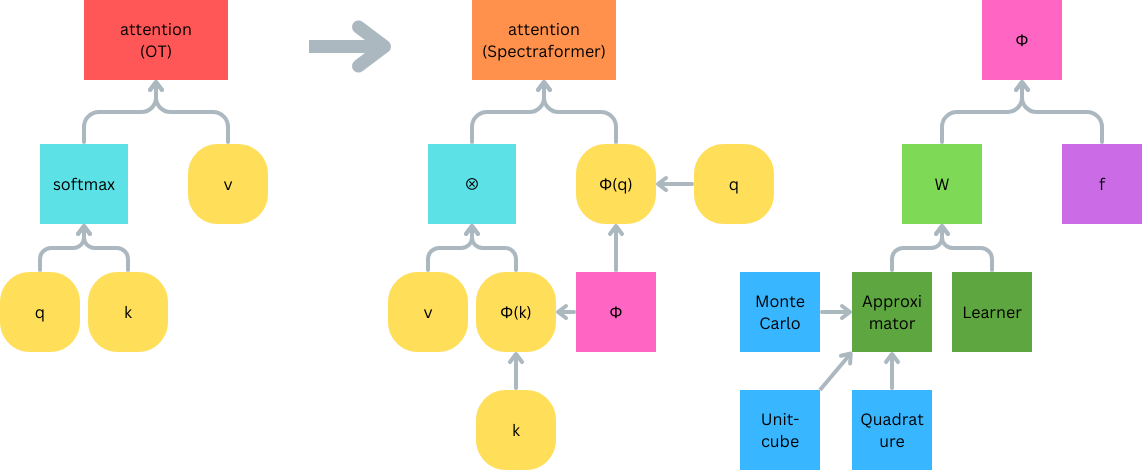
Figure 2: Spectraformer framework based on Equation 11

We term the matrix $\boldsymbol{W}$ as weight matrix instead of random matrix since although $\boldsymbol{W}$ acts like a random matrix ($\boldsymbol{\omega}_{i}\sim p(.)$, see Equation 10), it is not guaranteed to be one. In the case of weight matrix approximator, they approximate a random matrix and in the case of weight matrix learner, they parameterize a weight matrix, thereby implicitly learning a distribution $p(.)$ associated with such $\boldsymbol{W}$. The weight matrix is given in Definition 3.1.

Definition 3.1.

Provided that a matrix can substitute for a random matrix in Equation 11, and the solution for this equation given such matrix and $f$ as TrigRF being the solution for Equation 9, i.e., as an unbiased estimator of $\mathcal{K}$, and TrigRF being $f_{1}=f_{l}=\exp(-i\boldsymbol{\omega}^{T}\boldsymbol{x})$ (see Equation 10) then such a matrix is a weight matrix.

It follows from Definition 3.1 that for any weight matrix $\boldsymbol{W}$, $f=TrigRF$ is a valid component function. Spectraformer enables weight matrix approximation in terms of three families based on how they solve the intractable integral in Equation 9:

• Monte Carlo sampling-based weight matrix involves approximating the integral of Equation 9 using Monte Carlo sampling with the solution given by Equation 10 [19] with $\boldsymbol{W}$ being the ‘Base’ random matrix of $p(.)$, $\boldsymbol{\omega}_{i}\sim p(.)$. The random matrix $\boldsymbol{W}$ can be constructed more efficiently (either reducing time or space complexity) with FastFood [28]. The random matrix $\boldsymbol{W}$ can also be enforced to form geometrical couplings such as orthogonality to reduce approximation error with ORF, SORF [9]. Both these methods produce valid random matrices.

• Unit-cube sampling-based weight matrix transforms Equation 9 to an integral on the unit cube $[0,1]^{d}$, then performs the approximation with uniform and independent points, thus reducing variance. The first approach is QMC [25], where $\boldsymbol{W}:\boldsymbol{\omega}_{i}=\Phi^{-1}(\boldsymbol{t}_{i})$, $\Phi$ being the cumulative distribution function (CDF) associated with $p(.)$ and $\boldsymbol{t}_{i}$ being a low discrepancy sequence. $\Phi^{-1}(\boldsymbol{t}_{i})\sim p(.)$ whilst having a lower variance than direct sampling from $p(.)$. MM [26, 7] improves over QMC by replacing $\Phi^{-1}$ with a moment matching scheme $\widetilde{\Phi}^{-1}$ on $\Phi^{-1}$.

• Quadrature-based weight matrix uses quadrature rules with non-uniform deterministic weights. The main approach explored is SGQ [27] which uses one-dimensional Gaussian quadrature rule by assuming $\mathcal{K}$ factorizes with respect to the dimensions. Smolyak rule is further implemented to alleviate the curse of dimensionality.

[7] show that in various kernel benchmark datasets (among combination with TrigRF), QMC and ORF have consistently high performance. Due to the significant number of weight matrices in random features literature, we decide to cover only the most prominent ones. Appendix A.3 provides the technical details of the approximators discussed here and those that we left out.

Spectraformer also allows to learn weight matrices by learning $p(.)$ via parameterizing $\boldsymbol{W}$. [29] introduce several of these parametrization schemes, which are then adapted into the attention setting by [14]. The best performing method is via making the constituent matrices of FastFood learnable, which we term FastFood_L. In general, a weight matrix learner is valid as long as it can implicitly model any distribution. In addition the TrigRF, PosRF has also been applied on FastFood_L. Technical details and other learners we have not covered are explored in Appendix A.4. We now explore existing works which have developed from Rahimi and Recht [19] (see Equation 9, 10) and how they lead to the development of Spectraformer.

3.2 Component functions

Spectraformer incorporates component functions $f$ such as PosRF, OPRF, SADERF. Component functions in Spectraformer combine each weight matrix row $\boldsymbol{\omega}_{i}$ with the input $\boldsymbol{x}$. The base case of the component function is TrigRF. Component function is given in Definition 3.2

Definition 3.2.

A function of $\boldsymbol{x}$ with respect to $\boldsymbol{\omega}$ is a valid component function if and only if $\mathcal{K}\approx\phi_{\boldsymbol{\omega}}(\boldsymbol{x})^{T}\phi_{\boldsymbol{\omega}}(\boldsymbol{y})$ given that $\boldsymbol{\omega}_{i}\sim p(.)$ in Equation 10.

It follows that all component functions have provided theoretical guarantees given that $\boldsymbol{W}$ is a random matrix. In addition, PosRF, OPRF, and SADERF have also been proven theoretically to approximate $\mathcal{K}_{RBF}$ given $\boldsymbol{W}$ being the ORF.

While TrigRF[19] is the base component function and guarantees $\mathcal{K}(\boldsymbol{\delta})$ to be close to $\phi_{TrigRF}(\boldsymbol{x})\cdot\phi_{TrigRF}(\boldsymbol{y})$ due to uniform convergence, it is typically evaluated using only the real component of $\exp(-i\boldsymbol{\omega}_{j}^{T}\boldsymbol{x})$. This leads to $\cos$ and $\sin$ functions which can produce unstable behavior, especially when $K(\boldsymbol{\delta})$ is close to 0, where variance is infinite [8, 12]. Therefore, TrigRF is avoided in Spectraformer.

• PosRF [8] is introduced in Spectraformer as a simple modification over TrigRF to counter this instability. PosRF guarantees positive function output and its variance approaching 0 as $K(\boldsymbol{\delta})$ approaches 0. [12] generalize TrigRF and PosRF to GERF.

• OPRF [12] is one of the solution to the reduction of the variance equation of GERF. OPRF is both positive and bounded (whereas PosRF is positive and unbounded). [13] generalize GERF to dense matrix instead of scalar parameters leading to DERF.

• SADERF [13] is one of the solutions to the reduction of the variance equation of DERF. Whilst DERF has many solutions, they all rely on operations which are incompatible with many deep learning libraries on GPU and TPU like SVD and eigen decompositions. SADERF is an extension of GERF with a tighter variance bound on DERF.

The alternatives for component functions allow Spectraformer to approximate the RBF with $p(.)$ corresponding to the Gaussian. [13] and [12] show that SADERF-ORF is the SOTA combination followed by OPRF-ORF and PosRF-ORF. Technical details and other component function(s) not covered are explored in Appendix A.5.

Table 1: Summary of research gap in kernelized attention. Rows are the component functions, columns are the weight matrices. For each cell, the left item is the cited work for this combination for typical kernel tasks, while the right item is the cited work for Transformer-based tasks. $\times$ indicates no prior work for the combination. Spectraformer explores all combinations listed here, excluding ‘Base’ due to exhaustive work as seen in the table.

f	Monte Carlo			Unit-cube		Quadrature	Learner
	Base	ORF	SORF	QMC	MM	SGQ	FastFoodL
TrigRF	[19], [8]	[9], [8]	[9], $\times$	[25], $\times$	[26], $\times$	[27], $\times$	[29], [14]
PosRF	[8], [8]	[8], [8]	$\times$, $\times$	$\times$, $\times$	$\times$, $\times$	$\times$, $\times$	$\times$, [14]
OPRF	[12], [12]	[12], [12]	$\times$, $\times$	$\times$, $\times$	$\times$, $\times$	$\times$, $\times$	$\times$, $\times$
SADERF	[13], [13]	[13], [13]	$\times$, $\times$	$\times$, $\times$	$\times$, $\times$	$\times$, $\times$	$\times$, $\times$

3.3 Utility

There has been an unsystematic attempt at combining component functions and weight matrices. On one hand, most component functions have had theoretical and experimental results in combining with Base and ORF. On the other hand, most weight matrices have had results in combining with TrigRF or PosRF. This means that a lot of potential combinations have not been studied previously. Table 1 shows the wide research gap across 14 combinations which have never been studied in either the kernel or Transformer setting. Spectraformer highlights this research gap. Excluding TrigRF due to its instability and Base due to its underperformance, we conduct experiments on 18 combinations.

Spectraformer is a generic random feature framework that allows for the combination of any weight matrix with any component function provided that the weight matrix satisfies Definition 3.1 and the component function satisfies Definition 3.2. We note that Spectraformer is an experimental rather than a theoretical framework. Due to the large number of weight matrices and component functions, it is infeasible for the time being to derive a general mathematical proof for the bounds and convergence of Spectraformer. Therefore, we seek to validate its feasibility and show its ability to discover novel and performant combination via experimental results.

4 Results

4.1 Experiment Details

The LRA covers tasks of different sequence lengths, difficulty, and objective and it is designed to evaluate efficient Transformers, of which Spectraformer belongs to. Specifically, we evaluate the models on three LRA tasks: ListOps [30], Byte-Level Text Classification (using the IMDb review dataset) [31], and Byte-Level Document Retrieval (using the ACL Anthology Network dataset) [32]. All our models are experimented on Google Cloud Platform with n1-standard-4 (4 vCPUs, 15 GB RAM) and 1 NVIDIA T4 GPU. Our codebase is based on and includes the adapted or original implementation from [16], [14], [7], [8], [12], [13], [33] (Apache License, Version 2.0), [34] (Apache License, Version 2.0), [35], [36] (Apache License Version 2.0), [17].

Due to the significant number of models that are trained, we do not run the experiments on different seeds nor perform hyper-parameter tuning. The parameters are identical to [16] and chosen to limit the parameter count to account for the marked training time of multiple models. All the parameters for Spectraformer variants are kept identical for fair comparison, with the only difference being their random feature component. Our code is implemented in Python 3.12 and Pytorch, we use the Transformer base from [16]. Our hyperparameters are available in Table 5. The model name convention is [component function]-[weight matrix] (e.g., OPRF-FastFood_L).

Table 2: Experimental results of Spectraformer variants on the LRA benchmark. We report accuracy (on the test set), time (training time (hour)), and memory (peak memory consumption (GB)). $L$: ListOps, $T$: Text, $R$: Retrieval, and $\mu$ for the average of the three. The best variant (PosRF-MM) with highest average accuracy, and overall low training time/memory is higlighted in red. Existing RF techniques are cited in the model column. Novel combinations are marked by $\checkmark$ on the Novel column.

		Accuracy (%) $\uparrow$				Time (hour) $\downarrow$				Memory (GB) $\downarrow$
Novel	Model	L	T	R	$\mu$	L	T	R	$\mu$	L	T	R	$\mu$
	PosRF-ORF [8]	37.35	61.60	80.53	59.83	1.30	2.84	2.89	2.34	1.17	2.31	2.10	1.86
$\checkmark$	PosRF-SORF	22.98	63.31	65.52	50.60	1.29	2.81	2.83	2.31	1.17	2.31	2.10	1.86
$\checkmark$	PosRF-QMC	37.50	60.41	80.71	59.54	1.30	2.84	2.89	2.34	1.17	2.31	2.10	1.86
$\checkmark$	PosRF-SGQ	37.45	62.68	78.37	59.50	1.30	2.83	2.89	2.34	1.17	2.31	2.10	1.86
$\checkmark$	PosRF-MM	38.05	61.85	80.67	60.19	1.31	2.84	2.89	2.35	1.17	2.31	2.10	1.86
	PosRF-FastFoodL [14]	24.95	64.76	76.37	55.36	2.69	5.59	5.61	4.63	0.78	1.56	1.53	1.29
	OPRF-ORF [12]	37.50	59.35	80.90	59.25	1.61	3.45	3.50	2.86	1.36	2.71	2.56	2.21
$\checkmark$	OPRF-SORF	32.11	64.34	77.47	57.97	1.57	3.37	3.41	2.78	1.36	2.71	2.56	2.21
$\checkmark$	OPRF-QMC	38.41	60.32	80.80	59.84	1.61	3.46	3.51	2.86	1.36	2.71	2.56	2.21
$\checkmark$	OPRF-MM	38.71	60.39	80.45	59.85	1.61	3.46	3.51	2.86	1.36	2.71	2.56	2.21
$\checkmark$	OPRF-SGQ	22.53	61.34	79.29	54.39	1.60	3.45	3.47	2.84	1.36	2.71	2.56	2.21
$\checkmark$	OPRF-FastFoodL	37.40	64.04	78.32	59.92	2.81	5.84	5.86	4.84	0.85	1.69	1.67	1.40
	SADERF-ORF [13]	37.35	61.37	80.87	59.86	1.61	3.52	3.58	2.90	1.44	2.86	2.69	2.33
$\checkmark$	SADERF-SORF	32.31	64.49	76.43	57.74	1.58	3.44	3.49	2.84	1.44	2.86	2.69	2.33
$\checkmark$	SADERF-QMC	37.70	59.89	80.65	59.41	1.61	3.52	3.58	2.90	1.44	2.86	2.69	2.33
$\checkmark$	SADERF-MM	38.00	60.80	80.48	59.76	1.61	3.52	3.58	2.90	1.44	2.86	2.69	2.33
$\checkmark$	SADERF-SGQ	36.79	63.55	77.31	59.22	1.61	3.52	3.57	2.90	1.44	2.86	2.69	2.33
$\checkmark$	SADERF-FastFoodL	28.63	64.64	77.61	56.96	2.81	5.89	5.92	4.87	0.92	1.83	1.79	1.51

4.2 Comparison of Weight Matrix-Component Function Alternatives using Spectraformer

Our Spectraformer comparison results are available in Table 2. We now analyze the performance of component functions and weight matrices. We perform our analysis on both general trends of component functions across weight matrices and vice versa. We also make use of mean statistics (i.e., mean accuracy, mean training time, and mean peak memory consumption) which we give in brackets in the subsequent discussion.

Figure 3: Peak memory consumption (x-axis), accuracy (y-axis) on three textual LRA [15] tasks: ListOps, Text, Retrieval. Color indicates training time, the darker the faster, the brighter the slower (see legend). Models compared are the best Spectraformer variant (PosRF-MM) (boldened), the OT, and other efficient Transformers (RF and non-RF) in the literature. Values for non-RF Transformers are taken from [16].

Component functions. In terms of accuracy, SADERF (58.82%) typically performs better than OPRF (58.53%) and OPRF performs better than PosRF (57.50%) by small margin, agreeing with [12, 13]. However, SADERF (3.21 hours, 2.19 GB) and OPRF (3.17 hours, 2.24 GB) consistently take longer to train and have higher memory consumption than PosRF (2.71%, 1.76 GB) across weight matrices. This is likely due to OPRF and SADERF having additional computation of the L2 norm of the weight matrix which PosRF does not calculate.

Weight matrices. In terms of accuracy, SGQ (59.70%), ORF (59.64%), and QMC (59.59%) have the best performance. This is followed by MM (57.93%), FastFood_L (57.41%), and the worst being SORF (55.43%). In terms of training time, most weight matrices are rather uniform: SORF (2.64 hours) and MM, SGQ, QMC, ORF all at 2.69 hours. FastFood_L takes significant amount of time (4.78 hours). For peak memory consumption, FastFood_L is the most efficient at 1.73 GB whilst all other methods maintain a uniform value of 2.13 GB. FastFood_L reduces the space complexity at the cost of the time complexity. SORF reduces training time whilst compromising to a small extent its accuracy. This is interesting as it violates our initial assumptions that learners should perform better than approximators.

Best model. Overall, we find that PosRF-MM has the best performance, with the top accuracy (60.19%), top-3 training time (2.35 hours) and top-3 peak memory consumption (1.86 GB), outperforming the SOTA SADERF-ORF [13] (59.86%, 2.90 hours, and 2.33 GB) and OPRF-ORF [12] (59.25%, 2.86 hours, 2.21 GB) in the existing RF Transformer family. PosRF-MM achieves this performance due to the combination of both an efficient component function (PosRF) and performative weight matrix (MM). PosRF-MM has higher average accuracy (60.19) than the previous SOTA, SADERF-ORF (59.86), whilst having 23.4% faster training time, and 25.2% lower memory consumption. Our result demonstrates the viability of Spectraformer as a unifying random feature framework of Transformer.

Table 3: Comparison of the best Spectraformer variant (PosRF-MM), highlighted in red, against the OT and other efficient Transformers (RF and non-RF) in the literature. We report three metrics: accuracy (on the test set), time (training time (hour)), and memory (peak memory consumption (GB)). $L$ stands for ListOps, $T$ for Text, $R$ for Retrieval, and $\mu$ for the average of the three. Best results for each section and task are boldened.

	Accuracy (%) $\uparrow$				Time (hour) $\downarrow$				Memory (GB) $\downarrow$
Model	L	T	R	$\mu$	L	T	R	$\mu$	L	T	R	$\mu$
Original Transformer [1]	38.37	61.95	80.69	60.34	2.24	4.30	8.33	4.96	5.37	10.37	10.77	8.84
Nyströmformer [17]	38.51	64.83	80.52	61.29	0.71	0.71	1.29	0.90	1.37	1.21	2.39	1.66
Linformer [35]	37.45	58.93	78.19	58.19	0.60	0.65	1.13	0.79	0.99	0.99	1.89	1.29
Informer [36]	32.53	62.64	77.57	57.58	1.19	1.60	2.91	1.90	4.85	5.12	5.77	5.25
Reformer [33]	37.68	62.93	78.99	59.87	0.85	0.94	1.73	1.17	1.61	1.61	2.98	2.07
BigBird [37]	39.25	63.86	80.28	61.13	1.88	2.00	3.81	2.56	2.71	2.83	4.97	3.50
Skyformer [16]	38.69	64.70	82.06	61.82	1.29	1.02	1.86	1.39	1.75	1.59	3.15	2.16
PosRF-ORF [8]	37.35	61.60	80.53	59.83	1.30	2.84	2.89	2.34	1.17	2.31	2.10	1.86
OPRF-ORF [12]	37.50	59.35	80.90	59.25	1.61	3.45	3.50	2.86	1.36	2.71	2.56	2.21
SADERF-ORF [13]	37.35	61.37	80.87	59.86	0.00	3.52	3.58	2.36	0.00	2.86	2.69	1.85
PosRF-FastFoodL [14]	24.95	64.76	76.37	55.36	2.69	5.59	5.61	4.63	0.78	1.56	1.53	1.29
Spectraformer (PosRF-MM)	38.05	61.85	80.67	60.19	1.31	2.84	2.89	2.35	1.17	2.31	2.10	1.86

4.3 Comparison with other efficient Transformers

When comparing with other non-random feature Transformers, we observe that PosRF-MM performs comparatively against the OT whilst reducing memory consumption and training time significantly (see Figure 3 and Table 3). On ListOps and Retrieval, PosRF-MM and other Spectraformer variants perform on par with other non-RF efficient Transformers. Results for non-RF efficient Transformers (above the horizontal divider) in Table 3 are taken from [16]. Spectraformer does not outperform more performant Nyström-based transformers which are not based on random features. Having said that, we are the first to have conducted a comprehensive analysis of random feature methods in the Transformer via the Spectraformer framework, comparing it against other past works and the OT. Spectraformer can be extended in the future to include a larger range of component function and weight matrix options. We discuss limitations, and broader impact of our research in Appendix A.1.

5 Conclusion

We present Spectraformer, a framework for approximating and learning the attention kernel in the Transformer. Our paper generalizes past works and presents empirical findings on different component function and weight matrix combinations. We experiment with 18 combinations, of which 14 are novel. Novel combinations outperform the previous SOTA in the family for multiple tasks. Our best model, PosRF-MM, has higher average accuracy (60.19) than the previous SOTA, SADERF-ORF (59.86), whilst having 23.4% faster training time, and 25.2% lower memory consumption. This shows the viability of Spectraformer as a unifying random feature framework of Transformer.

Appendix A Appendix

A.1 Future work, limitations, and broader impact

Spectraformer provides an experimental framework for random features in the Transformer. However, we have not provided formal mathematical proofs for the bounds the these combinations due to the number of combinations discussed. We hope Spectraformer inspires future work to generalizes the proof in such a framework.

Spectraformer has covered a significant number of combinations, however, we have not covered all weight matrices and component functions in the literature. Spectraformer can serve as a foundation for further random feature Transformer research using the techiques not yet experimented with but covered in Appendices A.3, A.4, A.5.

Due to the significant number of experimented models, we are unable to perform hyper-parameter fine-tuning. Future work can benefit from extending the scope of the current research to other tasks, i.e., other non-textual LRA tasks (image classification, path-finder, and path-x) and short-context datasets/ tasks such as GLUE [38]. Transformer-based architecture can also benefit from Spectraformer. Past random feature Transformer works [12, 13] have experimented with conformer and vision Transformer with ViT. [39] provides a good foundation to extend our work. Spectraformer, although currently experimented in the Transformer setting, can also extend to non-parametric kernel classification. It could also benefit from ablation studies like the comparison variance in [14] or in [40]

Given the complex nature of language models in the ethical, energy, and societal domains, our work should be used responsibly  [41]

A.2 Related Work

Spectraformer is based on several theoretical assumptions and choice of mathematical framework and approach. This section discusses alternatives to the choices of Spectraformer. Specifically, Appendix A.2.1 discusses alternative kernelized formulations to Section 2.1; Appendix A.2.2 discusses alternative kernel approximation techniques to random features in Section A.2.2. There are also some component functions and weight matrices which are not covered in the experiments. We introduce them in the related work section in Appendices A.3, A.4, A.5.

A.2.1 Alternative Kernelized Attentions

In addition to the kernelized formulation of attention as shown in Section 2.1, based on our literature survey, we have identified the following three alternative kernel-based formulations of attention.

Nadaraya-Watson kernel estimator in integration form [42]: Given the Gaussian kernel, where the probability of a single variable and the joint probability of two variables are estimated using kernel density estimation with the Gaussian kernel, then we have the following equation:

$$\begin{array}[]{ll}\phi(\boldsymbol{\delta})&=exp(-||\boldsymbol{\delta}||^{2}/2\sigma^{2})\\ \hat{r}_{n}(\boldsymbol{k})&=\int\frac{\boldsymbol{v}p(\boldsymbol{v},\boldsymbol{k})}{p(\boldsymbol{k})}dv=\frac{\sum_{j=1}^{N}\hat{\boldsymbol{v}}_{j}\phi(\boldsymbol{k}-\boldsymbol{k}_{j})}{\sum_{j=1}^{N}\phi(\boldsymbol{k}-\boldsymbol{k}_{j})}\\ \hat{r}_{n}(\boldsymbol{q}_{i})&=\sum_{j=1}^{N}softmax(\boldsymbol{q}_{i}^{T}\boldsymbol{k}_{j}/\sigma^{2})\hat{\boldsymbol{v}}_{j}\end{array}$$ (12)

Equation 12 lays the foundation for FourierFormer - a Transformer with attention based on this formulation [42].

Gaussian decomposition [43]: the attention mechanism can also be decomposed into the Gaussian kernel directly from Equation 4 without appealing to the use of kernel estimator [43].

$$A_{i}=\sum_{j=1}^{N}\frac{1}{Z_{l}(\boldsymbol{q}_{i},\boldsymbol{K})}exp(\frac{-||\boldsymbol{q}_{i}-\boldsymbol{k}_{j}||^{2}_{2}}{2\sqrt{d_{k}}})exp(\frac{||\boldsymbol{q}_{i}||^{2}_{p=2}+||\boldsymbol{k}_{j}||^{2}_{p=2}}{2\sqrt{d_{k}}})\boldsymbol{v}_{j}$$ (13)

Equation 13 leads to Implicit Kernel Attention (IKA) - a Transformer with attention based on this formulation [43].

Non-local operation [44] is popular decomposition of attention in computer vision. This is the basis for Vision Transformer and related work. Non-local operation itself a generalisation of the non-local means used in image denoising [45]. Non-local operation is essentially an operation that operates on the entire input range, instead of a specific window which is characteristic of convolutional operations (see Equation 14). Indeed, the attention vector output $\boldsymbol{y}$ can be defined using $f$ which is the softmax (see Equation 15) in the non-local operation.

$$\mathbf{\boldsymbol{y}}_{i}=\frac{1}{C(\boldsymbol{x})}\sum_{\forall j}f(\boldsymbol{x}_{i},\boldsymbol{x}_{j})g(\boldsymbol{x}_{j})$$ (14)

$$\mathbf{\boldsymbol{y}}=softmax(\boldsymbol{x}^{T}\boldsymbol{W}_{\theta}^{T}\boldsymbol{W}_{\theta}\boldsymbol{x})g(\boldsymbol{x})$$ (15)

We will show that the non-local operation in Equation 14 is a generalisation of the Nadaraya-Watson kernel estimator. Specifically, when defining $C(\boldsymbol{x})=\sum_{l}\mathcal{K}(\boldsymbol{q}_{i},\boldsymbol{k}_{l}),f=\mathcal{K}(\boldsymbol{q}_{i},\boldsymbol{k}_{l}),g=\boldsymbol{v}_{j}$, then we obtain the original Nadaraya-Watson kernel estimator in Equation 4. The variety of kernel decompositions of attention demonstrate the robustness of the kernel interpretation of attention and hence opening up an alley in attention improvement through the lens of kernel.

A.2.2 Kernel Approximation Beyond Random Features

Kernel approximation is presented in Section 2.3 through the use of random features. However, there has been other kernel approximation techniques outside of random features. These include greedy basis selection [46], divide and conquer [47, 48], and nyström methods [49] (which led to the development of Skyformer [16] and Nyströmformer [17]).

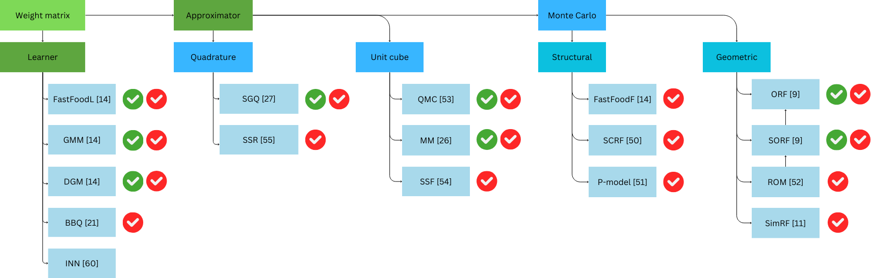
Figure 4: Spectraformer weight matrices. Red tick denotes techniques which have been explored in the literature. Green tick denotes techniques which are explored in this work.

A.3 Technical Details of Weight Approximators

Spectraformer weight matrices are shown in Figure 4. Weight matrices are either approximators or learners. There are three approaches to approximators: Monte Carlo sampling, Unit-cube sampling, and quadrature. We have discussed these approaches in detail in Section 3.1. Here we provide a more specific classification schemes for each method.

• Monte Carlo sampling-based weight matrices are improvements over Base and subdivided into two types: structural and geometric methods. Structural methods decompose the Base random matrices $P$ into smaller matrices which reduce time and/ or space complexity. Structural matrices includes FastFood_F, SCRF and P-Model. Among these, we have explored the learner variant FastFood_L of FastFood. Geometric methods enforce certain geometrical couplings along some dimensions in the construction of random matrices to reduce the approximation error. Geometric methods include: ROM (ORF, SORF) and SimRF. Among these, we have explored the main ROM variants - ORF and SORF.

• Unit-cube sampling-based weight matrices reformulate the Bochner integral in Equation 9 as Equation A.3 with uniform and independent points. This approach includes QMC, MM, and SSF. We have not covered SSF in our experiments.

• Quadrature-based weight matrices estimates the intractable integral using non-uniform weights with deterministic rules. There are two approaches: SGQ and SSR. We have not covered SSR in our experiments.

We now explore these weight matrices in the order specified above.

Base [19] is the direct sampling from a distribution $\boldsymbol{P}_{ij}\sim p$, corresponding to the kernel $\mathcal{K}$ without any additional adjustment, and in approximating the RBF, $P=G$ where $G$ is the normal distribution.

$$W_{Base}=\frac{1}{\sigma}\boldsymbol{P}$$ (16)

FastFood_F [28] makes use of Hadamard and diagonal matrices to speed up Gaussian matrices $G$ constructions for RFF in $O(n\log{d})$ (100 times faster) with $O(n)$ space (1000 times less space) given $n\geq d$ against Base. However, FastFood_F increases variance and approximation error and decreases the concentration bound.

$$W_{FastFood_{L}}=\frac{1}{\sigma}\boldsymbol{SHG\Pi HB}$$ (17)

where $\boldsymbol{H}$ is the Walsh-Hadamard matrix, $\boldsymbol{\Pi}\in\{0,1\}^{d*d}$ is a permutation matrix, and $\boldsymbol{S,G,B}$ are diagonal random matrices, with the diagonal entries being $\{+-1\}$ entries on $\boldsymbol{B}$, random Gaussian entries on $\boldsymbol{G}$, and a random scaling matrix on $\boldsymbol{S}$, $\boldsymbol{S}_{ii}=s_{i}||\boldsymbol{G}||^{-1/2}_{Frob}$, $s_{i}\sim(2\pi)^{\frac{-d}{2}}\boldsymbol{A}^{-1}_{d-1}r^{d-1}e^{-\frac{r^{2}}{2}}$.

SCRF (Signed Circulant Matrix Projection) [50] maintains a high matrix construction speed and $O(s)$ space ($s=t*d$) whilst maintaining the variance of Base, an improvement over FastFood_F. It does this by making use of circulant matrices.

$$\boldsymbol{W}_{SCRF}=[\boldsymbol{P}^{(1)},\boldsymbol{P}^{(2)},...,\boldsymbol{P}^{(t)}],t=d|D$$ (18)

where $\boldsymbol{P}^{(i)}$ is a signed circulant Gaussian matrix, with the first column of circulant random matrix $\boldsymbol{C}^{(i)_{[d]}}$ of $\boldsymbol{P}^{(i)}$ drawn randomly from a Gaussian distribution $\mathcal{N}(\boldsymbol{0},\boldsymbol{I}/\sigma^{2})$. The circulant matrix via Discrete Fourier Transform can be defined as:

$$\begin{array}[]{cc}\boldsymbol{C}=\frac{1}{m}\boldsymbol{F}^{*}diag(\boldsymbol{Fc})\boldsymbol{F}\\ \boldsymbol{F}=[e^{i\frac{2\pi}{m}kn}]^{m-1}_{k,n=0}\end{array}$$ (19)

P-Model [51] generalizes over both circulant matrices (including SCRF), FastFood_F, along with other Gaussian and semi-Gaussian structured matrix methods.

$$\boldsymbol{W}_{P_{model}}=[\boldsymbol{g^{T}P_{1}},\boldsymbol{g^{T}P_{2}},...,\boldsymbol{g^{T}P_{s}}]^{T}$$ (20)

where $\boldsymbol{g}\in\mathbb{R}^{a}$ is a Gaussian vector and a sequence of $m$ $\boldsymbol{P}_{i}\in\mathbb{R}^{a*d}$ matrices with L2 norm columns, where $P_{i}$ represents a P-model. Semi-Gaussian structured matrices including Toeplitz, Hankel, and other Toeplitz-like matrices are an open area of research for random matrices.

ORF (Orthogonal RF) [9] decreases the approximation error significantly compared to Base. This is done via replacing $G$ with a properly scaled random orthogonal matrix. However, generating orthogonal matrices become costly quickly as the number of dimensions increases.

$$\boldsymbol{W}_{ORF}=\frac{1}{\sigma}\boldsymbol{SQ}$$ (21)

where $\boldsymbol{Q}$ is a uniformly distributed random orthogonal matrix (on the Stiefel manifold) obtained from the QR decomposition of $\boldsymbol{G}$, the set of rows of $\boldsymbol{Q}$ forming a basis in $\mathbb{R}^{d}$, and $\boldsymbol{S}$ is a diagonal matrix with entries sampled i.i.d from the $\chi$-distribution with $d$ degrees of freedom, thus making the rows of $\boldsymbol{SQ}$ and $\boldsymbol{G}$ identically distributed.

SORF (Structured ORF) [9] decreases time and space complexity of ORF (from $O(d^{2})$ to $O(d\log{d})$ with almost no extra memory cost) by imposing structure on the orthogonal matrices, inspired by structural methods. SORF is unbiased with large $d$. We replace $\boldsymbol{S}$ with $\sqrt{d}$ and $\boldsymbol{Q}$ with structured matrix $\boldsymbol{HD}_{1}\boldsymbol{HD}_{2}\boldsymbol{HD}_{3}$

$$\boldsymbol{W}_{SORF}=\frac{\sqrt{d}}{\sigma}\boldsymbol{HD}_{1}\boldsymbol{HD}_{2}\boldsymbol{HD}_{3}$$ (22)

where $\boldsymbol{D}_{i}\in\mathbb{R}^{d*d},i=1,2,3$ is diagonal ’sign-flipping‘ matrices with diagonal entries sampled from the Rademacher distribution, $\boldsymbol{H}$ is the normalized Walsh-Hadamard matrix.

ROM (Random Orthogonal Embeddings) [52] generalizes SORF ($t=3$) to:

$$\boldsymbol{W}_{ROM}=\frac{\sqrt{d}}{\sigma}\prod_{i=1}^{t}\boldsymbol{SD}_{i}$$ (23)

where $\boldsymbol{S}$ is a class of $L_{2}$-normalized versions of Kronecker product matrices, of which the Hadamard $\boldsymbol{H}$ is a representative of, and $\boldsymbol{D}$ being independent diagonal matrices. When $\boldsymbol{S}=\boldsymbol{H}$ and $t=3$, we obtain SORF used in our experiments. Another ROM variant is S-Hybrid, which we do not experiment with, given as

$$\boldsymbol{W}_{S_{Hybrid}}=\boldsymbol{SD}_{k}^{(\mathcal{U})}\prod_{i=1}^{k-1}\boldsymbol{SD}_{i}^{(\mathcal{R})}$$ (24)

where $\boldsymbol{D}_{k}^{(\mathcal{U})}$ is a diagonal matrix with i.i.d. $Unif(\mathcal{S}^{1})$ on the unit circle of $\mathbb{C}$. When being used in the component function, instead of calculating $\phi(\boldsymbol{x})^{T}\phi(\boldsymbol{y})$ in Equation 10. We model the equation as $Real(\overline{\phi(\boldsymbol{x})}^{T}\phi(\boldsymbol{y}))$.

SimRF (Simplex RF) [11] is developed to be a positive RF with the most optimal solution, the MSE of which is the lowest in the geometric methods. This is an alternative to the ROM-based geometric methods. Two variants of SimRF are: weight-independent and weight-dependent. SimRF is defined as:

$$\boldsymbol{W}_{simp}=\boldsymbol{DSR}$$ (25)

where $\boldsymbol{D}\in\mathbb{R}^{d*d}=diag(\boldsymbol{\omega}_{i}),\boldsymbol{R}\in\mathbb{R}^{d*d}$ being a random orthogonal matrix drawn from Haar measure on $O(d)$ and $\boldsymbol{S}\in\mathbb{R}^{d*d}$ with row $\boldsymbol{s}_{i}$:

$$\boldsymbol{s}_{i}=\begin{cases}\sqrt{\frac{d}{d-1}}\boldsymbol{e}_{i}-\frac{\sqrt{d}+1}{(d-1)^{3/2}}(1,...,1,0)^{T}&1\leq i<d\\ \frac{1}{\sqrt{d-1}}(1,1,...,1,0)^{T}&i=d\end{cases}$$ (26)

being unit vectors which are manifestly normalized and subtend obtuse angles. SimRF variants are defined based on how $\boldsymbol{\omega}_{i}$ is constructed. For SimRF_indep, $\boldsymbol{\omega}_{i}\sim\chi_{d}$. For Sim_dep, we permit the random vector direction $\{\hat{\boldsymbol{\omega}}_{i}\}$ to be correlated with norms $\{\boldsymbol{\omega}_{i}\}$:

$$\boldsymbol{\omega}_{i}=-\frac{\sum_{j\neq i}\omega_{j}}{||\sum_{j\neq i}\omega_{j}||_{2}}\boldsymbol{\omega}_{i},i=1,...,d$$ (27)

QMC (Quasi-Monte Carlo) [25] evaluates on a low discrepancy sequence (e.g., Halton, Sobol’ Faure, and Niederreiter) of points instead of random points in Monte Carlo. Although the approximation error is only reduced minimally, QMC has been shown to perform better than MC in high dimensions and does not have undesirable clustering effect. To calculate QMC, we first assume that $p(\boldsymbol{x})=\prod^{d}_{j=1}p_{j}(\boldsymbol{x}_{j})$ factorizes with respect to the dimensions with $p_{j}(.)$ being a univariate density function. Then we define:

$$\Phi^{-1}(\boldsymbol{t})=\left(\Phi_{1}^{-1}\left(\boldsymbol{t}_{1}\right),\ldots,\Phi_{d}^{-1}\left(\boldsymbol{t}_{d}\right)\right)\in\mathbb{R}^{d}$$ (28)

where $\Phi_{j}$ being the cumulative distribution function of $p_{j}$, $\boldsymbol{t}_{1},\boldsymbol{t}_{2},...,\boldsymbol{t}_{s}\in[0,1]^{d}$ being a low discrepancy sequence, and $\boldsymbol{\omega}_{i}=\Phi^{-1}(\boldsymbol{t}_{i})$. We can thus transform the integral on $\mathbb{R}^{d}$ in Equation 9 to an integral on the unit cube $[0,1]^{d}$ as

$$\mathcal{K}(\boldsymbol{x}-\boldsymbol{x}^{\prime})=\int_{[0,1]^{d}}\exp\big{(}\mbox{i}(\boldsymbol{x}-\boldsymbol{x}^{\prime})^{\!\top}\Phi^{-1}(\boldsymbol{t})\big{)}\mbox{d}\boldsymbol{t}$$

The weight matrix then can be defined as:

$$\boldsymbol{W}_{\text{QMC}}=[\Phi^{-1}(\boldsymbol{t}_{1}),\Phi^{-1}(\boldsymbol{t}_{2}),\ldots,\Phi^{-1}(\boldsymbol{t}_{s})]^{\!\top}\in\mathbb{R}^{s\times d}\;.$$

QMC can be further improved by a sub-grouped based rank-one lattice construction which improved complexity [53].

MM (Moment Matching) [26] [7] improves over QMC by removing the undesirable clustering effect and having the same approximation error with less features. This is done by replacing $\Phi^{-1}$ with a moment matching scheme $\widetilde{\Phi}^{-1}$:

$$\boldsymbol{W}_{\text{MM}}=[\widetilde{\Phi}^{-1}(\boldsymbol{t}_{1}),\widetilde{\Phi}^{-1}(\boldsymbol{t}_{2}),\ldots,\widetilde{\Phi}^{-1}(\boldsymbol{t}_{s})]^{\!\top}\in\mathbb{R}^{s\times d}$$

where $\widetilde{\Phi}^{-1}(\boldsymbol{t}_{i})=\tilde{\boldsymbol{A}}^{-1}(\Phi^{-1}(\boldsymbol{t}_{i})-\tilde{\boldsymbol{\mu}})$ can be constructed using moment matching with sample mean $\tilde{\boldsymbol{\mu}}=\frac{1}{s}\sum_{i=1}^{s}\Phi^{-1}(\boldsymbol{t}_{i})$ and the square root of the sample covariance matrix $\tilde{\boldsymbol{A}}$ satisfying $\tilde{\boldsymbol{A}}\tilde{\boldsymbol{A}}^{\!\top}=\text{Cov}(\Phi^{-1}(\boldsymbol{t}_{i})-\tilde{\boldsymbol{\mu}})$.

SSF (Spherical Structured Features) [54] improves over QMC by including rotation-invariant kernel as well as in terms of complexity. Rotation-invariant property suggests the construction of feature maps using spherical equal weight approximation using Riesz s-energy on a d-dimensional sphere $\mathbb{S}^{d}:=\{\boldsymbol{x}\in\mathbb{R}^{d+1}|||\boldsymbol{x}||_{2}=1\}$. Specifically, we construct $\{\boldsymbol{v}_{i}\}^{s}_{i=1}$ asymptotically uniformly distributed on the sphere and obtain $\boldsymbol{V}:=[\boldsymbol{v}_{1},\boldsymbol{v}_{2},\ldots,\boldsymbol{v}_{s}]\in\mathbb{S}^{(d\times s}$, that $\Phi^{-1}(t)$ uses the one-dimensional QMC point, we have the weight matrix:

$$\boldsymbol{W}_{\text{SSF}}=[\Phi^{-1}(t)\boldsymbol{v}_{1},\Phi^{-1}(t)\boldsymbol{v}_{2},\ldots,\Phi^{-1}(t)\boldsymbol{v}_{s}]^{\!\top}\in\mathbb{R}^{s\times(d+1)},$$

SGQ (Sparse Grid Quadrature) [27] evolves from GQ. GQ (Gaussian Quadrature) [27] assumes that the kernel $k$ factorizes with respect to the dimensions and thus can be approximated by a one-dimensional Gaussian quadrature rule. However the total number of points $s$ scale exponentially with the dimensions. However GQ suffers form the curse of dimensionality. This is alleviated using Smolyak rule resulting in SGQ. Assuming the third-degree SGQ using symmetric univariate quadrature points $\left\{-\hat{p}_{1},0,\hat{p}_{1}\right\}$ with weights $(\hat{a}_{1},\hat{a}_{0},\hat{a}_{1})$, then we have:

$$\boldsymbol{W}_{\text{SGQ}}\!=\![\boldsymbol{0}_{d},\hat{p}_{1}\boldsymbol{e}_{1},\ldots,\hat{p}_{1}\boldsymbol{e}_{d},-\hat{p}_{1}\boldsymbol{e}_{1},\ldots,-\hat{p}_{1}\boldsymbol{e}_{d}]^{\!\top}\!\in\!\mathbb{R}^{(2d+1)\times d}\!$$

given that $\mathbb{e}_{i}$ is the d-dimensional standard basis vector with the i^th element being 1.

SSR (Spherical-Radial Rules) [55] transforms Equation 10 into a double integral over a hyper-sphere and the real line. This leads to the following approximation:

$$\boldsymbol{W}_{\text{SSR}}=\boldsymbol{\vartheta}\otimes\begin{bmatrix}(\boldsymbol{QV})^{\top}\\ -(\boldsymbol{Q}\boldsymbol{V})^{\top}\end{bmatrix}\in\mathbb{R}^{(2d+1)\times d},$$

where $\boldsymbol{\vartheta}=[\vartheta_{1},\vartheta_{2},\ldots,\vartheta_{s}]$, $\boldsymbol{V}=[\boldsymbol{v}_{1},\boldsymbol{v}_{2},\ldots,\boldsymbol{v}_{d+1}]$, $\vartheta\sim\chi(d+2)$ and $\{\boldsymbol{v}_{i}\}_{i=1}^{d+1}$ being vertices of a unit regular d-simplex randomly rotated by $\boldsymbol{Q}$ (a random orthogonal matrix).

A.4 Technical Details of Weight Learners

We give a non-mathematical definition of weight matrix learner in Section 3.1: weight matrix learner is any function which parameterize distributions. This allows for the discovery and future experimentation with other potential weight matrix learners in Spectraformer and random feature method in general. Weight matrix learner comes from a long line of work in kernel methods, namely, kernel learning via random features. Typically, a component function $f$ is chosen and a weight matrix $\boldsymbol{W}$ is produced via kernel approximation, providing us with the feature map $\phi$. $\phi$ can then be combined with input $\boldsymbol{x}$ and weight $\boldsymbol{v}$ to fit the learning objective. Kernel learning, however, imposes an additional objective: learning the weight matrix $\boldsymbol{W}$.

The approach to the dual objectives separates the kernel learning methods into two-stage and one-stage methods [7]. Two-stage methods (e.g., [56], [23], [57]) solves the dual objective separately: $\boldsymbol{W}$ is typically first learned via a kernel alignment scheme [58], then we solve for $\boldsymbol{v}$. One-stage methods (e.g., [14], [22]), on the other hand, solves the dual objective in parallel: $p(.)$ corresponding to $\boldsymbol{W}$ is parameterized then $\boldsymbol{v}$ is solved typically. It is not plausible to apply kernel alignment [58] on Transformer architectures. Therefore, only one-stage methods can be considered in the context of weight matrix learner. Two kernel learning methods, GMM and FastFood_L, have been experimented in the non-Transformer setting [29], then adapted into the Transformer setting [14]. DGM (Deep Generative Model) has also been effective in modeling distributions [59]. It too has been adapted by [14] for the Transformer setting. Due to the superior performance of FastFood_L in [14], we have only experimented with this technique. We now explore them.

FastFood_L (see Equation 17) is proposed to be learnable by [29] with two variations: FSARD (scaling matrix $\boldsymbol{S}$ previously sampled from chi-squared is made learnable) and FSGBARD (optimizes the marginal likelihood with respect to the diagonal matrices $\boldsymbol{G}$ and $\boldsymbol{B}$). It is further adapted by [14] to make $\boldsymbol{S}$ or $\boldsymbol{S},\boldsymbol{G},\boldsymbol{B}$ learnable parameters. In our experiments, we maintain the set up by [14].

GMM (Gaussian Mixture Model) [23, 24] is a known universal approximator of probability distribution. Specifically, we can consider $\boldsymbol{W}_{GMM}$ being composed of $s$ components, with each component $c$ (with $C$ total components) being a Gaussian with mean vector $\mu_{c}$ and covariance matrix $\Sigma_{c}$ and component weight $\pi_{c}$. $p(\boldsymbol{\omega})$ can then be approximated as $p(\boldsymbol{\omega})=\sum_{c=1}^{C}\pi_{c}\mathcal{N}(\mu_{c},\Sigma_{c})$ [14]. Assuming $\pi_{c}=\frac{1}{C}$, the weight matrix with learnable weights $\Sigma$ and $\mu$ can be parameterized as [14]:

$$\boldsymbol{W}_{GMM}=[\Sigma_{1}n+\mu_{1},...,\Sigma_{C}n+\mu_{C}]^{T},n\sim\mathcal{N}(\boldsymbol{0},\boldsymbol{I})$$ (29)

Another formulation of GMM is proposed in [29] in combination with FastFood, albeit it extends beyond constructing the weight matrix.

DGM (Deep Generative Model) [59] allows for a generic distribution modeling using neural network. DGM is initially proposed to make differentiating sampling processes possible via the reparametrization trick, where the generator $g$ creates samples from the target distribution $\boldsymbol{\omega}_{m}=g(\boldsymbol{n}_{m})$ via transforming from a noise distribution $\boldsymbol{n}_{m}\sim p_{0}(.)$.

In addition to the techniques discussed above, there are also some other prominent one-stage methods (e.g., INN, BBQ). INN (Invertible Neural Network) [60] is another universal approximator of probability distribution, consisting of invertible operations transforming samples from a known distribution to a different more complex distribution. BBQ (Black Box Quantile) [22] follows the QMC scheme and models $\Phi^{-1}$ using parameterized quantile function.

A.5 Technical Details of Component Functions

Figure 5: Spectraformer component functions. Red tick denotes techniques which have been explored in the literature. Green tick denotes techniques which are explored in this work.

Component functions discussed in Section 3.2 all belong to CDERF. However, there are other component functions including DIRF and HRF (see Figure 5) which we do not explore in our experiments. We now investigate the theoretical details of these component functions, the CDERF family is introduced in their order of discovery.

CDERF (Complex dense exponential random feature) is given in Equation 30, where $\boldsymbol{\omega},\boldsymbol{x}\in\mathbb{R}^{d}$, $p=\mathcal{N}(0,1)^{d}$, $k\in\{1,2\}$ and $\mathbb{S}_{d_{c}}$ being a set of $d*d$ complex symmetric matrices. The parameters and constraints of different CDERF functions are specified in Table 4:

$$f_{DE}^{(k)}(\boldsymbol{\omega},\boldsymbol{x})=Real(D\exp(\boldsymbol{\omega}^{T}\boldsymbol{A}\boldsymbol{\omega}+\boldsymbol{\omega}^{T}\boldsymbol{B}^{(k)}\boldsymbol{x}+\boldsymbol{x}^{T}\boldsymbol{C}^{(k)}\boldsymbol{x}))$$ (30)

Table 4: CDERF component functions

	$\boldsymbol{A}$	$\boldsymbol{B}^{(1)}$	$\boldsymbol{B}^{(2)}$	$\boldsymbol{C}^{(1)}$	$\boldsymbol{C}^{(2)}$	$D$	$\boldsymbol{x}$	$\boldsymbol{y}$
CDERF	$\mathbb{S}_{d_{C}}$	$\mathbb{C}^{d*d}$		$\mathbb{C}^{d*d}$		$\mathbb{R}$	$\boldsymbol{x}$	$\boldsymbol{y}$
DERF [13]	$\mathbb{S}_{d}$	$\mathbb{R}^{d*d}$		$\mathbb{R}^{d*d}$		$\mathbb{R}$	$\boldsymbol{x}$	$\boldsymbol{y}$
SADERF [13]	$A_{GE}\boldsymbol{I}_{d}$	$B_{GE}\boldsymbol{I}_{d}$		$C_{GE}\boldsymbol{I}_{d}$		$D_{GE}$	$\Psi\boldsymbol{x}$	$\Psi^{-1}\boldsymbol{y}$
GERF [12]	$A_{GE}\boldsymbol{I}_{d}$	$B_{GE}^{(1)}\boldsymbol{I}_{d}$	$B_{GE}^{(2)}\boldsymbol{I}_{d}$	$C_{GE}\boldsymbol{I}_{d}$		$D_{GE}$	$\boldsymbol{x}$	$\boldsymbol{y}$
TrigRF [19]	$0\boldsymbol{I}_{d}$	$i\boldsymbol{I}_{d}$	$-i\boldsymbol{I}_{d}$	$0\boldsymbol{I}_{d}$		$1$	$\boldsymbol{x}$	$\boldsymbol{y}$
PosRF [8]	$0\boldsymbol{I}_{d}$	$1\boldsymbol{I}_{d}$		$-1\boldsymbol{I}_{d}$		$1$	$\boldsymbol{x}$	$\boldsymbol{y}$
OPRF [12]	$0\boldsymbol{I}_{d}$	$1\boldsymbol{I}_{d}$		$-1\boldsymbol{I}_{d}$		$1$	$\boldsymbol{x}$	$\boldsymbol{y}$

TrigRF (Trigonometric RF) [19] is the base RFF implementation.

$$\begin{array}[]{c}f_{TrigRF}^{(1)}(\boldsymbol{\omega},\boldsymbol{x})=\sqrt{2}\cos(\boldsymbol{\omega}^{T}\boldsymbol{x}+\boldsymbol{b})\\ f_{TrigRF}^{(2)}(\boldsymbol{\omega},\boldsymbol{y})=\sqrt{2}\sin(\boldsymbol{\omega}^{T}\boldsymbol{y}+\boldsymbol{b})\\ \boldsymbol{b}\sim Uniform(0,2\pi)\end{array}$$ (31)

The use of the trigonometric sine and cosine functions leads to unstable behavior when the inputs have negative dimension-values. This can be further exacerbated when the values TrigRF try to approximate are close to 0 (since most values are of low significance). This causes the variance to approach infinity [8, 12]. Therefore, we do not want to use TrigRF to perform kernel approximation in attention.

PosRF (Positive RF) [8] fixes the problem of TrigRF by enforcing positive component function output in the softmax. The variance of PosRF (in contrast to the variance of TrigRF approaching infinity) approaches 0 as the approximated value of the Softmax kernel approaches 0. PosRF has two forms: Positive RF Base (PosRF-B) (see Equation 32) and Positive RF Hyperbolic (PosRF-Hyp), which is multi-component, i.e., Equation 11: $l=2$, (see Equation 33).

$$\begin{array}[]{c}f_{PosRF_{B}}(\boldsymbol{\omega},\boldsymbol{x})=\exp(\boldsymbol{\omega}^{T}\boldsymbol{x}-\frac{||\boldsymbol{x}||^{2}}{2})\end{array}$$ (32)

$$\begin{array}[]{ll}f_{1,PosRF_{Hyp}}(\boldsymbol{\omega},\boldsymbol{x})=\exp(\boldsymbol{\omega}^{T}\boldsymbol{x}-||\boldsymbol{x}||^{2})\\ f_{2,PosRF_{Hyp}}(\boldsymbol{\omega},\boldsymbol{x})=\exp(-\boldsymbol{\omega}^{T}\boldsymbol{x}-||\boldsymbol{x}||^{2})\end{array}$$ (33)

We only use PosRF-B in our experiments.

GERF (Generalized exponential RF) [12] generalizes both TrigRF and PosRF with Equation 34.

$$\begin{array}[]{c}f_{GERF}^{(1)}(\boldsymbol{\omega},\boldsymbol{x})=D\exp(A||\boldsymbol{\omega}||^{2}+B\boldsymbol{\omega}^{T}\boldsymbol{x}+\boldsymbol{C}||\boldsymbol{x}||^{2})\\ f_{GERF}^{(2)}(\boldsymbol{\omega},\boldsymbol{y})=D\exp(\boldsymbol{A}||\boldsymbol{\omega}||^{2}+sB\boldsymbol{\omega}^{T}\boldsymbol{y}+\boldsymbol{C}||\boldsymbol{y}||^{2})\\ \\ Re(1-4A)>0,\boldsymbol{B}=\sqrt{s(1-4\boldsymbol{A})}\\ \boldsymbol{C}=-(s+1)/2,D=(\sqrt[4]{1-4\boldsymbol{A}})^{d}\\ \boldsymbol{A}\in\mathbb{C},s\in\{-1,+1\}\end{array}$$ (34)

where $\sqrt{.}$ and $\sqrt[n]{.}$ denoting a principal root with a complex argument

OPRF (Optimized positive RF) [12] is the solution to the minimization of the variance of GERF. Specifically it is defined as Equation 34 with $s=+1$, $||\boldsymbol{x}+\boldsymbol{y}||^{2}>0$, and $\boldsymbol{A}\in\mathbb{R}$ defined in terms of $p^{*}$ as:

$$\begin{array}[]{cc}\boldsymbol{A}=(1-1/p^{*})/8\\ p^{*}=(\sqrt{(2||\boldsymbol{x}+\boldsymbol{y}||^{2}+d)^{2}+8d||\boldsymbol{x}+\boldsymbol{y}||^{2}}-2||\boldsymbol{x}+\boldsymbol{y}||^{2}-d)\\ /(4||\boldsymbol{x}+\boldsymbol{y}||^{2})\end{array}$$ (35)

Whilst PosRF is not bounded, OPRF is. OPRF can provide $e^{60}$ $\times$ variance reduction in estimating the Softmax compared to TrigRF [12].

DERF (Dense-exponential random features) [13] extends GERF and replace $\boldsymbol{A},\boldsymbol{B},\boldsymbol{C}$ with dense matrices. DERF is CDERF when $\boldsymbol{B},C$ are in the real instead of the complex plane. Minimizing the variance of DERF leads to two approaches: ADERF and SDERF. However both these approaches rely on SVD and eigen decompositions which are not extensively supported on GPU and deep learning libraries. Therefore SADERF is proposed.

SADERF (simplified ADERF) [13] is a special case of ADERF and extends GERF, requiring only basic unary operations in addition.

$$\begin{array}[]{c}f_{SADE}^{(1)}(\boldsymbol{\omega},\boldsymbol{x})=f_{GE}^{(1)}(\boldsymbol{\omega},\Psi\boldsymbol{x}),f_{SADE}^{(2)}(\boldsymbol{\omega},\boldsymbol{y})=f_{GE}^{(2)}(\boldsymbol{\omega},\Psi^{-1}\boldsymbol{y})\\ \Psi_{l,l}^{*}=(\sum_{j}(\boldsymbol{y}_{l}^{(i)})^{2}/\sum_{i}(\boldsymbol{x}_{l}^{(i)})^{2})^{1/4}\end{array}$$ (36)

DIRF (Discretely-induced random features) [12] are based on the assumption of $p(\boldsymbol{\omega})$ being a discrete distribution with $\boldsymbol{\omega}_{1},...,\boldsymbol{\omega}_{d}$ being i.i.d., $\mathbb{P}(\boldsymbol{\omega}_{l}=k)=p_{k}$, $\sum_{k=0}^{\infty}p_{k}=1$, $p_{k}>0,k\in\{0\}\cup\mathbb{N}$. By making use of the Taylor series, we can define DIRF as:

$$f_{DI}(\boldsymbol{\omega},\boldsymbol{x})=\exp(-\frac{||\boldsymbol{x}||^{2}}{2})\prod_{l=1}^{d}\boldsymbol{x}_{i}^{\boldsymbol{\omega}_{l}}(\boldsymbol{\omega}_{l}!)^{\frac{-1}{2}}p_{\boldsymbol{\omega}_{l}}^{\frac{-1}{2}}$$ (37)

DIRF has two variations: PoisRF (Poisson RF) which requires $p(.)$ to be the Poisson distribution and GeomRF (Geometric RF) which requires $p(.)$ to be the geometric distribution. Since the many weight matrices introduced in Section 3.1 do not readily approximate these distributions, we decide to leave DIRF out of the paper.

HRF (Hybrid RF) [10] combines multiple base estimators, similar to multiple kernel learning methods [61], in order to provide the most accurate approximation in regions of interest. Choromanski et al. on solving softmax approximation using HRF. HRF is constructed using a weighted combination $\epsilon$ of $p+1$ base estimators $\hat{SM}^{k}(\boldsymbol{x},\boldsymbol{y})$ and $\lambda$-coefficients, $\Lambda$ $p$ binary estimators $\lambda^{k}:\mathbb{R}^{d}\times\mathbb{R}^{d}\rightarrow[0,1]$, both constructed independently:

$$\hat{SM}^{\epsilon,\Lambda}=\sum_{k=1}^{p}\hat{\lambda}^{k}(\boldsymbol{x},\boldsymbol{y})\hat{SM}^{k}(\boldsymbol{x},\boldsymbol{y})+(1-\sum_{k=1}^{p}\hat{\lambda}^{k}(\boldsymbol{x},\boldsymbol{y}))\hat{SM}^{p+1}(\boldsymbol{x},\boldsymbol{y})$$ (38)

Since HRF requires the base estimators $SM(\boldsymbol{x},\boldsymbol{y})$ to be unbiased, the easiest solution is the complex exponential $\hat{SM}^{cexp}_{m}$ which can be derived directly from the expectation of the softmax as follows:

$$\begin{array}[]{cc}\hat{SM}^{cexp}_{m}(\boldsymbol{x},\boldsymbol{y})=\psi^{m}_{A}(\boldsymbol{x})^{T}\psi^{m}_{(\boldsymbol{A}^{T})^{-1}}(\boldsymbol{y})\\ \psi^{m}_{\boldsymbol{M}}(u)=\frac{1}{\sqrt{m}}\exp(-\frac{(\boldsymbol{Mu})^{2}}{2})\\ (\exp(\boldsymbol{\omega}^{T}_{i}\boldsymbol{Mu}),...,\exp(\boldsymbol{\omega}_{m}^{T}\boldsymbol{Mu}))^{T},\boldsymbol{\omega}_{i}\sim\mathcal{N}(\boldsymbol{0},\boldsymbol{I}_{d})\end{array}$$ (39)

To construct $\lambda$-coefficients, three methods are proposed: simultaneous accurate approximation of both small and large values, Gaussian Lambda Coefficients, and adaption to data admitting clustering structure.

A.6 Experimental Details in Spectraformer

Table 5: Hyper-parameters for Spectraformer, following the setting from [16] due to limited computational power. $L$ stands for ListOps, $T$ for Text, and $R$ for Retrieval. The seed that can be used to reproduce our experiments is 42.

	L	T	R
Embedding dim.	64	64	64
Transformer dim	64	64	64
Hidden dim	128	128	128
Head dim	32	32	32
Num. heads	2	2	2
Num. layers	2	2	2
Vocabulary size	32	512	512
Sequence length	2000	4000	4000
Dropout rate	0.1	0.1	0.1
Att. dropout rate	0.1	0.1	0.1
Pooling mode	mean
Batch size	32	32	16
Learning rate	0.0001	0.0001	0.0002
Warmup steps	1000	80	800
Learning rate decay	linear
Weight decay	0	0	0
Evaluation freq.	500	500	1000
Num. epochs	50k	50K	50k
Num. init steps	1k	3K	3k
Num. eval steps	62	200	300
Patience	10	10	10
Num. features	128	128	128

References

- Vaswani et al. [2017] Ashish Vaswani, Noam Shazeer, Niki Parmar, Jakob Uszkoreit, Llion Jones, Aidan N Gomez, Ł ukasz Kaiser, and Illia Polosukhin. Attention is all you need. In I. Guyon, U. Von Luxburg, S. Bengio, H. Wallach, R. Fergus, S. Vishwanathan, and R. Garnett, editors, Advances in Neural Information Processing Systems, volume 30. Curran Associates, Inc., 2017. URL https://proceedings.neurips.cc/paper_files/paper/2017/file/3f5ee243547dee91fbd053c1c4a845aa-Paper.pdf.
- Han et al. [2023] Kai Han, Yunhe Wang, Hanting Chen, Xinghao Chen, Jianyuan Guo, Zhenhua Liu, Yehui Tang, An Xiao, Chunjing Xu, Yixing Xu, Zhaohui Yang, Yiman Zhang, and Dacheng Tao. A survey on vision transformer. IEEE Transactions on Pattern Analysis and Machine Intelligence, 45(1):87–110, 2023. doi: 10.1109/TPAMI.2022.3152247.
- Lin et al. [2022] Tianyang Lin, Yuxin Wang, Xiangyang Liu, and Xipeng Qiu. A survey of transformers. AI Open, 3:111–132, 2022. ISSN 2666-6510. doi: https://doi.org/10.1016/j.aiopen.2022.10.001. URL https://www.sciencedirect.com/science/article/pii/S2666651022000146.
- Tsai et al. [2019] Yao-Hung Hubert Tsai, Shaojie Bai, Makoto Yamada, Louis-Philippe Morency, and Ruslan Salakhutdinov. Transformer dissection: An unified understanding for transformer’s attention via the lens of kernel. In Kentaro Inui, Jing Jiang, Vincent Ng, and Xiaojun Wan, editors, Proceedings of the 2019 Conference on Empirical Methods in Natural Language Processing and the 9th International Joint Conference on Natural Language Processing (EMNLP-IJCNLP), pages 4344–4353, Hong Kong, China, 11 2019. Association for Computational Linguistics. doi: 10.18653/v1/D19-1443. URL https://aclanthology.org/D19-1443.
- Hofmann et al. [2008] Thomas Hofmann, Bernhard Schölkopf, and Alexander J. Smola. Kernel methods in machine learning. The Annals of Statistics, 36(3):1171 – 1220, 2008. doi: 10.1214/009053607000000677. URL https://doi.org/10.1214/009053607000000677.
- Katharopoulos et al. [2020] Angelos Katharopoulos, Apoorv Vyas, Nikolaos Pappas, and François Fleuret. Transformers are RNNs: Fast autoregressive transformers with linear attention. In Hal Daumé III and Aarti Singh, editors, Proceedings of the 37th International Conference on Machine Learning, volume 119 of Proceedings of Machine Learning Research, pages 5156–5165. PMLR, 13–18 Jul 2020. URL https://proceedings.mlr.press/v119/katharopoulos20a.html.
- Liu et al. [2022] Fanghui Liu, Xiaolin Huang, Yudong Chen, and Johan A. K. Suykens. Random features for kernel approximation: A survey on algorithms, theory, and beyond. IEEE Transactions on Pattern Analysis and Machine Intelligence, 44(10):7128–7148, 2022. doi: 10.1109/TPAMI.2021.3097011.
- Choromanski et al. [2021] Krzysztof Marcin Choromanski, Valerii Likhosherstov, David Dohan, Xingyou Song, Andreea Gane, Tamas Sarlos, Peter Hawkins, Jared Quincy Davis, Afroz Mohiuddin, Lukasz Kaiser, David Benjamin Belanger, Lucy J Colwell, and Adrian Weller. Rethinking attention with performers. In International Conference on Learning Representations, 2021. URL https://openreview.net/forum?id=Ua6zuk0WRH.
- Yu et al. [2016] Felix Xinnan X Yu, Ananda Theertha Suresh, Krzysztof M Choromanski, Daniel N Holtmann-Rice, and Sanjiv Kumar. Orthogonal random features. In D. Lee, M. Sugiyama, U. Luxburg, I. Guyon, and R. Garnett, editors, Advances in Neural Information Processing Systems, volume 29. Curran Associates, Inc., 2016. URL https://proceedings.neurips.cc/paper_files/paper/2016/file/53adaf494dc89ef7196d73636eb2451b-Paper.pdf.
- Choromanski et al. [2022] Krzysztof Marcin Choromanski, Han Lin, Haoxian Chen, Arijit Sehanobish, Yuanzhe Ma, Deepali Jain, Jake Varley, Andy Zeng, Michael S Ryoo, Valerii Likhosherstov, Dmitry Kalashnikov, Vikas Sindhwani, and Adrian Weller. Hybrid random features. In International Conference on Learning Representations, 2022. URL https://openreview.net/forum?id=EMigfE6ZeS.
- Reid et al. [2023] Isaac Reid, Krzysztof Marcin Choromanski, Valerii Likhosherstov, and Adrian Weller. Simplex random features. In Andreas Krause, Emma Brunskill, Kyunghyun Cho, Barbara Engelhardt, Sivan Sabato, and Jonathan Scarlett, editors, Proceedings of the 40th International Conference on Machine Learning, volume 202 of Proceedings of Machine Learning Research, pages 28864–28888. PMLR, 23–29 Jul 2023. URL https://proceedings.mlr.press/v202/reid23a.html.
- Likhosherstov et al. [2022] Valerii Likhosherstov, Krzysztof M Choromanski, Kumar Avinava Dubey, Frederick Liu, Tamas Sarlos, and Adrian Weller. Chefs'random tables: Non-trigonometric random features. In S. Koyejo, S. Mohamed, A. Agarwal, D. Belgrave, K. Cho, and A. Oh, editors, Advances in Neural Information Processing Systems, volume 35, pages 34559–34573. Curran Associates, Inc., 2022. URL https://proceedings.neurips.cc/paper_files/paper/2022/file/df2d62b96a4003203450cf89cd338bb7-Paper-Conference.pdf.
- Likhosherstov et al. [2023] Valerii Likhosherstov, Krzysztof Marcin Choromanski, Kumar Avinava Dubey, Frederick Liu, Tamas Sarlos, and Adrian Weller. Dense-exponential random features: Sharp positive estimators of the gaussian kernel. In Thirty-seventh Conference on Neural Information Processing Systems, 2023. URL https://openreview.net/forum?id=S0xrBMFihS.
- Chowdhury et al. [2022] Sankalan Pal Chowdhury, Adamos Solomou, Kumar Avinava Dubey, and Mrinmaya Sachan. Learning the transformer kernel. Transactions on Machine Learning Research, 2022. ISSN 2835-8856. URL https://openreview.net/forum?id=tLIBAEYjcv.
- Tay et al. [2021] Yi Tay, Mostafa Dehghani, Samira Abnar, Yikang Shen, Dara Bahri, Philip Pham, Jinfeng Rao, Liu Yang, Sebastian Ruder, and Donald Metzler. Long range arena : A benchmark for efficient transformers. In International Conference on Learning Representations, 2021. URL https://openreview.net/forum?id=qVyeW-grC2k.
- Chen et al. [2021] Yifan Chen, Qi Zeng, Heng Ji, and Yun Yang. Skyformer: Remodel self-attention with gaussian kernel and nystr\”om method. In A. Beygelzimer, Y. Dauphin, P. Liang, and J. Wortman Vaughan, editors, Advances in Neural Information Processing Systems, 2021. URL https://openreview.net/forum?id=pZCYG7gjkKz.
- Xiong et al. [2021] Yunyang Xiong, Zhanpeng Zeng, Rudrasis Chakraborty, Mingxing Tan, Glenn Fung, Yin Li, and Vikas Singh. Nyströmformer: A nyström-based algorithm for approximating self-attention. Proceedings of the AAAI Conference on Artificial Intelligence, 35(16):14138–14148, May 2021. doi: 10.1609/aaai.v35i16.17664. URL https://ojs.aaai.org/index.php/AAAI/article/view/17664.
- Galassi et al. [2021] Andrea Galassi, Marco Lippi, and Paolo Torroni. Attention in natural language processing. IEEE Transactions on Neural Networks and Learning Systems, 32(10):4291–4308, 2021. doi: 10.1109/TNNLS.2020.3019893.
- Rahimi and Recht [2007] Ali Rahimi and Benjamin Recht. Random features for large-scale kernel machines. In J. Platt, D. Koller, Y. Singer, and S. Roweis, editors, Advances in Neural Information Processing Systems, volume 20. Curran Associates, Inc., 2007. URL https://proceedings.neurips.cc/paper_files/paper/2007/file/013a006f03dbc5392effeb8f18fda755-Paper.pdf.
- Rudin [1990] Walter Rudin. The Basic Theorems of Fourier Analysis, chapter 1, pages 1–34. John Wiley & Sons, Ltd, 1990. ISBN 9781118165621. doi: https://doi.org/10.1002/9781118165621.ch1. URL https://onlinelibrary.wiley.com/doi/abs/10.1002/9781118165621.ch1.
- Schölkopf and Smola [2018] Bernhard Schölkopf and Alexander J Smola. Kernels. In Learning with Kernels: Support Vector Machines, Regularization, Optimization, and Beyond. The MIT Press, 06 2018. ISBN 9780262256933. doi: 10.7551/mitpress/4175.003.0005. URL https://doi.org/10.7551/mitpress/4175.003.0005.
- Tompkins et al. [2019] Anthony Tompkins, Ransalu Senanayake, Philippe Morere, and Fabio Ramos. Black box quantiles for kernel learning. In Kamalika Chaudhuri and Masashi Sugiyama, editors, Proceedings of the Twenty-Second International Conference on Artificial Intelligence and Statistics, volume 89 of Proceedings of Machine Learning Research, pages 1427–1437. PMLR, 16–18 Apr 2019. URL https://proceedings.mlr.press/v89/tompkins19a.html.
- Wilson and Adams [2013] Andrew Wilson and Ryan Adams. Gaussian process kernels for pattern discovery and extrapolation. In Sanjoy Dasgupta and David McAllester, editors, Proceedings of the 30th International Conference on Machine Learning, volume 28 of Proceedings of Machine Learning Research, pages 1067–1075, Atlanta, Georgia, USA, 17–19 Jun 2013. PMLR. URL https://proceedings.mlr.press/v28/wilson13.html.
- Oliva et al. [2016] Junier B. Oliva, Avinava Dubey, Andrew G. Wilson, Barnabas Poczos, Jeff Schneider, and Eric P. Xing. Bayesian nonparametric kernel-learning. In Arthur Gretton and Christian C. Robert, editors, Proceedings of the 19th International Conference on Artificial Intelligence and Statistics, volume 51 of Proceedings of Machine Learning Research, pages 1078–1086, Cadiz, Spain, 09–11 May 2016. PMLR. URL https://proceedings.mlr.press/v51/oliva16.html.
- Avron et al. [2016] Haim Avron, Vikas Sindhwani, Jiyan Yang, and Michael W. Mahoney. Quasi-monte carlo feature maps for shift-invariant kernels. Journal of Machine Learning Research, 17(120):1–38, 2016. URL http://jmlr.org/papers/v17/14-538.html.
- Shen et al. [2017] Weiwei Shen, Zhihui Yang, and Jun Wang. Random features for shift-invariant kernels with moment matching. In Proceedings of the Thirty-First AAAI Conference on Artificial Intelligence, AAAI’17, page 2520–2526. AAAI Press, 2017.
- Dao et al. [2017] Tri Dao, Christopher M De Sa, and Christopher Ré. Gaussian quadrature for kernel features. In I. Guyon, U. Von Luxburg, S. Bengio, H. Wallach, R. Fergus, S. Vishwanathan, and R. Garnett, editors, Advances in Neural Information Processing Systems, volume 30. Curran Associates, Inc., 2017. URL https://proceedings.neurips.cc/paper_files/paper/2017/file/62f91ce9b820a491ee78c108636db089-Paper.pdf.
- Le et al. [2013] Quoc Le, Tamas Sarlos, and Alexander Smola. Fastfood - computing hilbert space expansions in loglinear time. In Sanjoy Dasgupta and David McAllester, editors, Proceedings of the 30th International Conference on Machine Learning, volume 28 of Proceedings of Machine Learning Research, pages 244–252, Atlanta, Georgia, USA, 17–19 Jun 2013. PMLR. URL https://proceedings.mlr.press/v28/le13.html.
- Yang et al. [2015] Zichao Yang, Andrew Wilson, Alex Smola, and Le Song. A la Carte – Learning Fast Kernels. In Guy Lebanon and S. V. N. Vishwanathan, editors, Proceedings of the Eighteenth International Conference on Artificial Intelligence and Statistics, volume 38 of Proceedings of Machine Learning Research, pages 1098–1106, San Diego, California, USA, 09–12 May 2015. PMLR. URL https://proceedings.mlr.press/v38/yang15b.html.
- Nangia and Bowman [2018] Nikita Nangia and Samuel Bowman. ListOps: A diagnostic dataset for latent tree learning. In Silvio Ricardo Cordeiro, Shereen Oraby, Umashanthi Pavalanathan, and Kyeongmin Rim, editors, Proceedings of the 2018 Conference of the North American Chapter of the Association for Computational Linguistics: Student Research Workshop, pages 92–99, New Orleans, Louisiana, USA, June 2018. Association for Computational Linguistics. doi: 10.18653/v1/N18-4013. URL https://aclanthology.org/N18-4013.
- Howard and Ruder [2018] Jeremy Howard and Sebastian Ruder. Universal language model fine-tuning for text classification. In Iryna Gurevych and Yusuke Miyao, editors, Proceedings of the 56th Annual Meeting of the Association for Computational Linguistics (Volume 1: Long Papers), pages 328–339, Melbourne, Australia, July 2018. Association for Computational Linguistics. doi: 10.18653/v1/P18-1031. URL https://aclanthology.org/P18-1031.
- Radev et al. [2013] Dragomir R. Radev, Pradeep Muthukrishnan, Vahed Qazvinian, and Amjad Abu-Jbara. The acl anthology network corpus. Language Resources and Evaluation, 47(4):919–944, 2013. ISSN 1574020X, 15728412. URL http://www.jstor.org/stable/42636383.
- Kitaev et al. [2020] Nikita Kitaev, Lukasz Kaiser, and Anselm Levskaya. Reformer: The efficient transformer. In International Conference on Learning Representations, 2020. URL https://openreview.net/forum?id=rkgNKkHtvB.
- Thomas et al. [2018] Anna Thomas, Albert Gu, Tri Dao, Atri Rudra, and Christopher Ré. Learning compressed transforms with low displacement rank. In S. Bengio, H. Wallach, H. Larochelle, K. Grauman, N. Cesa-Bianchi, and R. Garnett, editors, Advances in Neural Information Processing Systems, volume 31. Curran Associates, Inc., 2018. URL https://proceedings.neurips.cc/paper_files/paper/2018/file/8e621619d71d0ae5ef4e631ad586334f-Paper.pdf.
- Wang et al. [2020] Sinong Wang, Belinda Z. Li, Madian Khabsa, Han Fang, and Hao Ma. Linformer: Self-attention with linear complexity, 2020.
- Zhou et al. [2021] Haoyi Zhou, Shanghang Zhang, Jieqi Peng, Shuai Zhang, Jianxin Li, Hui Xiong, and Wancai Zhang. Informer: Beyond efficient transformer for long sequence time-series forecasting. Proceedings of the AAAI Conference on Artificial Intelligence, 35(12):11106–11115, May 2021. doi: 10.1609/aaai.v35i12.17325. URL https://ojs.aaai.org/index.php/AAAI/article/view/17325.
- Zaheer et al. [2020] Manzil Zaheer, Guru Guruganesh, Kumar Avinava Dubey, Joshua Ainslie, Chris Alberti, Santiago Ontanon, Philip Pham, Anirudh Ravula, Qifan Wang, Li Yang, and Amr Ahmed. Big bird: Transformers for longer sequences. In H. Larochelle, M. Ranzato, R. Hadsell, M.F. Balcan, and H. Lin, editors, Advances in Neural Information Processing Systems, volume 33, pages 17283–17297. Curran Associates, Inc., 2020. URL https://proceedings.neurips.cc/paper_files/paper/2020/file/c8512d142a2d849725f31a9a7a361ab9-Paper.pdf.
- Linzen et al. [2018] Tal Linzen, Grzegorz Chrupała, and Afra Alishahi, editors. GLUE: A Multi-Task Benchmark and Analysis Platform for Natural Language Understanding, Brussels, Belgium, November 2018. Association for Computational Linguistics. doi: 10.18653/v1/W18-5446. URL https://aclanthology.org/W18-5446.
- Jeevan and Sethi [2022] Pranav Jeevan and Amit Sethi. Resource-efficient hybrid x-formers for vision. In 2022 IEEE/CVF Winter Conference on Applications of Computer Vision (WACV), pages 3555–3563, 2022. doi: 10.1109/WACV51458.2022.00361.
- Yao et al. [2023] Junwen Yao, N. Benjamin Erichson, and Miles E. Lopes. Error estimation for random fourier features. In Francisco Ruiz, Jennifer Dy, and Jan-Willem van de Meent, editors, Proceedings of The 26th International Conference on Artificial Intelligence and Statistics, volume 206 of Proceedings of Machine Learning Research, pages 2348–2364. PMLR, 25–27 Apr 2023. URL https://proceedings.mlr.press/v206/yao23a.html.
- Weidinger et al. [2021] Laura Weidinger, John Mellor, Maribeth Rauh, Conor Griffin, Jonathan Uesato, Po-Sen Huang, Myra Cheng, Mia Glaese, Borja Balle, Atoosa Kasirzadeh, Zac Kenton, Sasha Brown, Will Hawkins, Tom Stepleton, Courtney Biles, Abeba Birhane, Julia Haas, Laura Rimell, Lisa Anne Hendricks, William Isaac, Sean Legassick, Geoffrey Irving, and Iason Gabriel. Ethical and social risks of harm from language models, 2021.
- Nguyen et al. [2022] Tan Nguyen, Minh Pham, Tam Nguyen, Khai Nguyen, Stanley Osher, and Nhat Ho. Fourierformer: Transformer meets generalized fourier integral theorem. In S. Koyejo, S. Mohamed, A. Agarwal, D. Belgrave, K. Cho, and A. Oh, editors, Advances in Neural Information Processing Systems, volume 35, pages 29319–29335. Curran Associates, Inc., 2022. URL https://proceedings.neurips.cc/paper_files/paper/2022/file/bc968adbdff4a2551649d464b83f264a-Paper-Conference.pdf.
- Song et al. [2021] Kyungwoo Song, Yohan Jung, Dongjun Kim, and Il-Chul Moon. Implicit kernel attention. Proceedings of the AAAI Conference on Artificial Intelligence, 35(11):9713–9721, May 2021. doi: 10.1609/aaai.v35i11.17168. URL https://ojs.aaai.org/index.php/AAAI/article/view/17168.
- Wang et al. [2018] Xiaolong Wang, Ross Girshick, Abhinav Gupta, and Kaiming He. Non-local neural networks. In 2018 IEEE/CVF Conference on Computer Vision and Pattern Recognition, pages 7794–7803, 2018. doi: 10.1109/CVPR.2018.00813.
- Buades et al. [2005] A. Buades, B. Coll, and J.-M. Morel. A non-local algorithm for image denoising. In 2005 IEEE Computer Society Conference on Computer Vision and Pattern Recognition (CVPR’05), volume 2, pages 60–65 vol. 2, 2005. doi: 10.1109/CVPR.2005.38.
- Smola and Schökopf [2000] Alex J. Smola and Bernhard Schökopf. Sparse greedy matrix approximation for machine learning. In Proceedings of the Seventeenth International Conference on Machine Learning, ICML ’00, page 911–918, San Francisco, CA, USA, 2000. Morgan Kaufmann Publishers Inc. ISBN 1558607072.
- Hsieh et al. [2014] Cho-Jui Hsieh, Si Si, and Inderjit Dhillon. A divide-and-conquer solver for kernel support vector machines. In Eric P. Xing and Tony Jebara, editors, Proceedings of the 31st International Conference on Machine Learning, volume 32 of Proceedings of Machine Learning Research, pages 566–574, Bejing, China, 22–24 Jun 2014. PMLR. URL https://proceedings.mlr.press/v32/hsieha14.html.
- Zhang et al. [2013] Yuchen Zhang, John Duchi, and Martin Wainwright. Divide and conquer kernel ridge regression. In Shai Shalev-Shwartz and Ingo Steinwart, editors, Proceedings of the 26th Annual Conference on Learning Theory, volume 30 of Proceedings of Machine Learning Research, pages 592–617, Princeton, NJ, USA, 12–14 Jun 2013. PMLR. URL https://proceedings.mlr.press/v30/Zhang13.html.
- Williams and Seeger [2000] Christopher Williams and Matthias Seeger. Using the nyström method to speed up kernel machines. In T. Leen, T. Dietterich, and V. Tresp, editors, Advances in Neural Information Processing Systems, volume 13. MIT Press, 2000. URL https://proceedings.neurips.cc/paper_files/paper/2000/file/19de10adbaa1b2ee13f77f679fa1483a-Paper.pdf.
- Feng et al. [2015] Chang Feng, Qinghua Hu, and Shizhong Liao. Random feature mapping with signed circulant matrix projection. In Proceedings of the 24th International Conference on Artificial Intelligence, IJCAI’15, page 3490–3496. AAAI Press, 2015. ISBN 9781577357384.
- Choromanski and Sindhwani [2016] Krzysztof Choromanski and Vikas Sindhwani. Recycling randomness with structure for sublinear time kernel expansions. In Maria Florina Balcan and Kilian Q. Weinberger, editors, Proceedings of The 33rd International Conference on Machine Learning, volume 48 of Proceedings of Machine Learning Research, pages 2502–2510, New York, New York, USA, 20–22 Jun 2016. PMLR. URL https://proceedings.mlr.press/v48/choromanski16.html.
- Choromanski et al. [2017] Krzysztof M Choromanski, Mark Rowland, and Adrian Weller. The unreasonable effectiveness of structured random orthogonal embeddings. In I. Guyon, U. Von Luxburg, S. Bengio, H. Wallach, R. Fergus, S. Vishwanathan, and R. Garnett, editors, Advances in Neural Information Processing Systems, volume 30. Curran Associates, Inc., 2017. URL https://proceedings.neurips.cc/paper_files/paper/2017/file/bf8229696f7a3bb4700cfddef19fa23f-Paper.pdf.
- LYU et al. [2020] Yueming LYU, Yuan Yuan, and Ivor Tsang. Subgroup-based rank-1 lattice quasi-monte carlo. In H. Larochelle, M. Ranzato, R. Hadsell, M.F. Balcan, and H. Lin, editors, Advances in Neural Information Processing Systems, volume 33, pages 6269–6280. Curran Associates, Inc., 2020. URL https://proceedings.neurips.cc/paper_files/paper/2020/file/456048afb7253926e1fbb7486e699180-Paper.pdf.
- Lyu [2017] Yueming Lyu. Spherical structured feature maps for kernel approximation. In Doina Precup and Yee Whye Teh, editors, Proceedings of the 34th International Conference on Machine Learning, volume 70 of Proceedings of Machine Learning Research, pages 2256–2264. PMLR, 06–11 Aug 2017. URL https://proceedings.mlr.press/v70/lyu17a.html.
- Munkhoeva et al. [2018] Marina Munkhoeva, Yermek Kapushev, Evgeny Burnaev, and Ivan Oseledets. Quadrature-based features for kernel approximation. In S. Bengio, H. Wallach, H. Larochelle, K. Grauman, N. Cesa-Bianchi, and R. Garnett, editors, Advances in Neural Information Processing Systems, volume 31. Curran Associates, Inc., 2018. URL https://proceedings.neurips.cc/paper_files/paper/2018/file/6e923226e43cd6fac7cfe1e13ad000ac-Paper.pdf.
- Yu et al. [2015] Felix X. Yu, Sanjiv Kumar, Henry Rowley, and Shih-Fu Chang. Compact nonlinear maps and circulant extensions, 2015.
- Bullins et al. [2018] Brian Bullins, Cyril Zhang, and Yi Zhang. Not-so-random features. In International Conference on Learning Representations, 2018. URL https://openreview.net/forum?id=Hk8XMWgRb.
- Wang et al. [2015] Tinghua Wang, Dongyan Zhao, and Shengfeng Tian. An overview of kernel alignment and its applications. Artificial Intelligence Review, 43:179–192, 2015.
- Kingma and Welling [2013] Diederik P. Kingma and Max Welling. Auto-encoding variational bayes. CoRR, abs/1312.6114, 2013. URL https://api.semanticscholar.org/CorpusID:216078090.
- Xu et al. [2021] Da Xu, Chuanwei Ruan, Evren Korpeoglu, Sushant Kumar, and Kannan Achan. A temporal kernel approach for deep learning with continuous-time information, 2021.
- Bach et al. [2004] Francis R. Bach, Gert R. G. Lanckriet, and Michael I. Jordan. Multiple kernel learning, conic duality, and the smo algorithm. In Proceedings of the Twenty-First International Conference on Machine Learning, ICML ’04, page 6, New York, NY, USA, 2004. Association for Computing Machinery. ISBN 1581138385. doi: 10.1145/1015330.1015424. URL https://doi.org/10.1145/1015330.1015424.