Learning Invariant Causal Mechanism from Vision-Language Models
Abstract
Pre-trained large-scale models have become a major research focus, but their effectiveness is limited in real-world applications due to diverse data distributions. In contrast, humans excel at decision-making across various domains by learning reusable knowledge that remains invariant despite environmental changes in a complex world. Although CLIP, as a successful vision-language pre-trained model, demonstrates remarkable performance in various visual downstream tasks, our experiments reveal unsatisfactory results in specific domains. Our further analysis with causal inference exposes the current CLIP model’s inability to capture the invariant causal mechanisms across domains, attributed to its deficiency in identifying latent factors generating the data. To address this, we propose the Invariant Causal Mechanism of CLIP (CLIP-ICM), an algorithm designed to provably identify invariant latent factors with the aid of interventional data, and perform accurate prediction on various domains. Theoretical analysis demonstrates that our method has a lower generalization bound in out-of-distribution (OOD) scenarios. Experimental results showcase the outstanding performance of CLIP-ICM.
1 Introduction
Pre-trained large-scale models have garnered sustained attention as a prominent research direction (Chen et al., 2020; He et al., 2022; Radford et al., 2021). The primary objective of these models is to provide a unified representation for various downstream tasks (Bengio et al., 2014).
In real-world applications, these models are supposed to be flexibly adapted to more diverse scenarios, encompassing data distribution different from those encountered during training (Torralba & Efros, 2011; Fang et al., 2013; Beery et al., 2018; Gulrajani & Lopez-Paz, 2020; Abbe et al., 2023). Consequently, the generalization ability of pre-train models is restricted, leading to the formation of out-of-distribution (OOD) problems.
Existing approaches including (Ganin et al., 2016; Li et al., 2018; Arjovsky et al., 2020; Sagawa* et al., 2019) have been designed to mitigate the challenges associated with OOD scenarios. While these methods have achieved a certain degree of success in addressing related issues, the OOD problem still persists and demands urgent resolution (Gulrajani & Lopez-Paz, 2020). Providentially, vision-language representation learning presents promising alternatives (Frome et al., 2013; Socher et al., 2013). Vary from traditional label-based visual pre-train models and unsupervised pre-train models, vision-language representation learning enriches representations by aligning images with natural language descriptions, offering a wealth of semantic information. Among the most widely adopted vision-language pre-train models, Contrastive Language-Image Pretraining (CLIP) (Radford et al., 2021) stands out for its ability to seamlessly transfer to various visual downstream tasks in a zero-shot manner, yielding commendable performance.
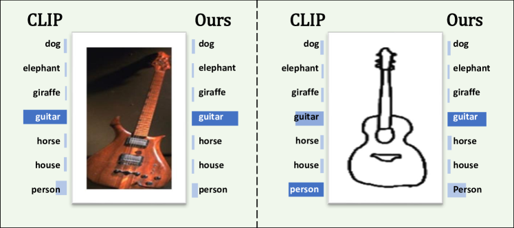
To assess the efficacy of CLIP in addressing OOD issues, we investigate CLIP’s classification performance across different domains within the VLCS (Fang et al., 2013) dataset. However, experimental results reveal inconsistent performance of CLIP when applied to various domains. In particular, CLIP shows poor performance when faced with the OOD problem in zero-shot scenarios. In other words, the representations generated by CLIP do not capture all the invariant features shared across domains. The human cognitive process involves highly abstract representations. In the process of understanding the world, humans tend to encapsulate the mechanisms of the physical world as a collection of causal relationships (Schölkopf et al., 2021). Humans are capable of making robust judgments across various environments based on features that remain invariant across different domains (Peters et al., 2015; Arjovsky et al., 2020; Ahuja et al., 2022a). However, CLIP fails to gain the capacity to make this kind of judgment.
To further validate our results, we construct a structural causal model (SCM) (Pearl, 2009) for the prediction process of CLIP in OOD scenarios. Additionally, we demonstrate that the current prediction process fails to capture invariant causal mechanisms. Furthermore, we identify and substantiate the sufficient and necessary conditions for capturing invariant causal mechanisms. Based on these conditions, we propose CLIP-ICM which could effectively capture the invariant causal mechanisms across various domains. Subsequently, we conduct a generalization analysis of the model based on Rademacher complexity, demonstrating that CLIP-ICM has a lower generalization bound compared to CLIP. This observation implies a superior generalization ability of our method. Experimental results on commonly used OOD datasets corroborate the outstanding effectiveness of our approach in achieving superior performance under zero-shot and linear-probe conditions.
Our contributions could be summarized as follows:
-
•
We discover that CLIP in OOD scenarios always suffers from the poor performance problem. Then, we establish a CLIP-related SCM from a causal perspective, demonstrating its inability to capture invariant causal mechanisms. Subsequently, we identify the sufficient and necessary conditions for capturing invariant causal mechanisms.
-
•
We give a theoretical analysis of identifying invariant latent factors in feature representations under a specific condition, and propose a method called CLIP-ICM to satisfy that specific condition. Furthermore, based on Rademacher complexity, we prove that CLIP-ICM exhibits a lower generalization bound relative to CLIP, indicating the superior generalization performance of our method.
-
•
The experimental results verify that CLIP-ICM is very effective compared to the state-of-the-art and can effectively improve the performance of CLIP in dealing with zero-shot OOD problems. Meanwhile, we conduct a series of ablation studies to validate the effectiveness of our proposed CLIP-ICM.
2 Related Works
Vision-Language Pre-training.
Incorporating language with the visual modality has been a long-standing issue extensively researched (Frome et al., 2013; Socher et al., 2013; Norouzi et al., 2014; Elhoseiny et al., 2013). In recent years, multi-modal pre-training models led by CLIP (Radford et al., 2021) and ALIGN (Jia et al., 2021) have achieved significant success. The objective of this approach is to enable cross-modal learning by mapping language and visual modals into the same embedding space. Recently, researches have been focusing on improving the OOD performance when adapting CLIP to downstream tasks (Gao et al., 2023; Zhou et al., 2022a, b; Shu et al., 2023). (Gao et al., 2023) propose CLIP-Adapter to perform fine-tuning with feature adapters. (Zhou et al., 2022a, b) propose to learn dynamic prompts to improve the OOD performance of CLIP. (Shu et al., 2023) propose a fine-tuning method that adapts CLIP models to OOD situations. In our work, we analyze the reason for poor OOD generalization ability of previous methods. We propose CLIP-ICM to facilitate CLIP-related methods by learning invariant causal mechanisms.
Causal Representation Learning.
The latent factor hypothesis assumes that a set of latent factors generate the observational data (Bishop, 1998). A core task in causal representation learning is to provably identify these latent factors (Bengio et al., 2014; Schölkopf et al., 2021; Schoelkopf et al., 2012). Additionally, the issue of identification is commonly referred to as the Independent Component Analysis (ICA) problem (Hyvärinen & Oja, 2000), which aims to separate independent signals from those mixed during observation. While the problem of ICA has been proven to be achievable in the linear case (Hyvärinen & Oja, 2000), non-linear ICA has been shown to be impossible without inductive biases relying on auxiliary labels (Hyvärinen & Pajunen, 1999; Locatello et al., 2019; Hyvarinen & Morioka, 2017; Locatello et al., 2020), imposing sparsity (Schölkopf et al., 2021; Lachapelle et al., 2022), or restricting the function class (Zimmermann et al., 2022).
Importantly, many of these approaches are variations of the Variational Autoencoder framework (Kingma & Welling, 2013). Attention is also drawn to identification work on discriminative models (Zimmermann et al., 2022; Kügelgen et al., 2021; Roeder et al., 2021). Similar to our work, (Kügelgen et al., 2021) also uses data augmentations to obtain the invariant factors, and we provide a detailed comparison with them in Appendix H. Specifically, (Roeder et al., 2021) demonstrate that discriminative representation learning methods, including classification and contrastive learning (Oord et al., 2019; Radford et al., 2021), can identify latent factors with an affine transformation.(Daunhawer et al., 2023) also provide identifiability results for multimodal contrastive learning, demonstrating the recovery of shared factors in a more general multimodal setup beyond the multi-view settings previously studied.
While the studies mentioned above concentrate on scenarios with only observational data, an increasing number of studies are now focusing on cases where interventional data is available (Ahuja et al., 2023; Buchholz et al., 2023; Squires et al., 2023). We approach from a similar perspective and propose a method to identify latent factors through interventions in the data. Compared to the method they proposed, we introduce a simple and effective way to utilize intervention data to identify the invariant features of CLIP.
Out-of-distribution Generaliztion.
It is evident in many cases that the performance of deep learning methods is weakened when applied to different distributions (Beery et al., 2018; Taori et al., 2020). Studies have been conducted to address the OOD generalization issues (Arjovsky et al., 2020; Ahuja et al., 2020; Gulrajani & Lopez-Paz, 2020; Miller et al., 2021; Abbe et al., 2023; Chen et al., 2023). One important branch of work aims to find the invariant causal mechanisms across domains (Arjovsky et al., 2020; Peters et al., 2016; Suter et al., 2019; Ahuja et al., 2020, 2022a; Chen et al., 2023); the core of aforementioned works is inspired by the invariance principle from causality (Pearl, 2009; Pearl & Bareinboim, 2014; Schölkopf et al., 2021). (Robey et al., 2021; Wald et al., 2021; Li et al., 2024) also incorporate with SCM when analyzing the OOD problem, we provide a detailed comparison with them in Appendix H. Vision-language pre-trained models, such as CLIP (Radford et al., 2021), exhibit impressive performance across various domains. However, recent works emphasize that adapting CLIP with task-specific data comes at the cost of OOD generalization ability (Shu et al., 2023; Gao et al., 2023; Pham et al., 2023). In our investigation of the invariant causal mechanisms of CLIP, we theoretically demonstrate that our method exhibits superior OOD generalization ability.
3 Preliminaries
3.1 Contrastive Language-Image Pre-training
We begin by revisiting the framework for vision-language joint training, as introduced in (Radford et al., 2021). Let be an arbitrary image, and be a text sequence to describe this image, where denotes the image space and represents the text space. CLIP aims to train an image encoder and a text encoder to map and into a joint embedding space . Given a mini-batch of image-text pairs , the objective for learning and is achieved by the following contrastive loss functions:
| (1) | ||||
| (2) |
where is a temperature hyperparameter. Minimizing these two loss functions can maximize the similarity between the embeddings of the correct image pairs , while minimizing the similarity between the wrong image pairs .
The CLIP model facilitates zero-shot predictions for unknown classification tasks with classes. For each class , a corresponding text prompt is employed, e.g., ”a photo of a [CLASS]” where [CLASS] represents the name of class . The probability that an image sample belongs to class is computed using the formula:
| (3) |
Another commonly employed predictive approach, known as linear evaluation, aims to learn a classifier with the parameters of the pre-trained model fixed. Using linear evaluation, the probability that a sample belongs to class is calculated as follows:
| (4) |
In this work, to assess the prediction performance of CLIP, we use to denote the estimated probability by CLIP, where is the parameter.
3.2 Out-Of-Distribution Generalization
Next, we formalize the setting when CLIP is used across various domains. We consider supervised training data gathered from a set of environments : , where represents the dataset from environment . Here, is the number of instances in environment , and is the joint distribution of the sample and label in environment , is the image and is the corresponding class label. The goal of OOD generalization is to find a predictor , estimated by parameter , that performs well across various unseen environments in , where . Specifically, the objective is to minimize the OOD risk:
| (5) |
where represents the risk of the predictor in environment . The OOD typically encompasses two primary scenarios: domain shift, where the training and test data originate from different domains; and open class, where the test data introduces new classes not encountered during training. In the case of domain shift, the class label remains constant across all environments. Conversely, in open class scenarios, the distribution of the sample remains fixed across all environments.
3.3 Background in Causality
The SCMs are used to describe the causal variables and their relationships. The definition of SCM is:
Definition 3.1.
(Structural Causal Model (Pearl, 2009))
1. A set of background or exogenous variables, representing factors outside the model, which nevertheless affect relationships within the model.
2. A set of endogenous variables, assumed to be observable. Each of these variables is functionally dependent on some subset of . Here, means the set of parent nodes of the endogenous variable .
3. A set of functions such that each determines the value of , . These functions are also known as causal mechanisms.
4. A joint probability distribution over .
The SCMs can be represented by Directed Acyclic Graphs (DAG) (Glymour et al., 2016). In the DAG, the arrow denotes that changes in the value of directly cause changes in . However, this relationship does not hold in the reverse order.
In statistical learning, we can only identify the association by , indicating the correlation between variable and . However, in causal learning, our focus shifts to understanding the genuine causal mechanisms, specifically how the intervention of the variable influences another variable . This form of intervention is modeled by replacing the causal mechanisms with a constant value, denoted by the -operator (Bareinboim et al., 2022). In essence, while reflects statistical associations, signifies a causal relationship by explicitly considering the intervention in the causal structure.
4 Main Results
In this section, we first conduct a series of experiments using CLIP and observe various performances across different domains. Particularly, in certain domains, the classification results are notably poor. To investigate the prediction process of CLIP in various domains, we explicitly model the causal relationships between latent factors and observation data with SCM. Through analysis, we infer that the unsatisfactory results stem from the inherent lack of transferability of the causal mechanisms. Subsequently, we establish that the causal mechanism becomes transferable only when variant factors are observable, and the prediction depends solely on the invariant factors. Based on this insight, we propose to utilize interventional data to identify the latent factors. We propose CLIP-ICM, an algorithm to identify the invariant latent factors and conduct predictions based on them. Furthermore, we demonstrate that our method leads to a lower OOD generalization bound.
4.1 Motivation Experiment
We follow the standard zero-shot prediction protocol of CLIP (Radford et al., 2021) and report the prediction accuracy on different domains in the VLCS (Torralba & Efros, 2011) dataset and report the results in Table 1.
| Algorithm | C | L | S | V | Avg |
|---|---|---|---|---|---|
| CLIP Zero-shot | 99.90.0 | 70.10.0 | 73.50.0 | 86.10.0 | 82.4 |
| CLIP Linear-probe | 93.70.2 | 65.40.2 | 76.40.2 | 79.10.3 | 78.7 |
It is evident from the table that accuracy varies across different domains. Specifically, when performing prediction with both zero-shot and linear-probe manner, in the L domain, classification accuracy is notably lower compared to other domains. Consequently, according to Equation 5, the OOD risk of CLIP is high, indicating the unsatisfactory OOD generalization ability of CLIP.
4.2 Causal Analysis
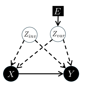
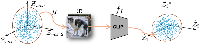
To further investigate the reason for the unsatisfactory OOD generalization ability of CLIP, we establish the SCM as in Figure 2(a). In the proposed SCM, is the image, and is the text description. and are latent factors that generate the image and label according to the latent factor hypothesis (Bishop, 1998). We also introduce an additional exogenous variable denotes the environment, i.e. the domain (Pearl & Bareinboim, 2014). is the set of latent factors that remain constant across various domains, and is the set of latent factors that depend on environments. It is noteworthy that the variables and are not observable. The edge and the edge denote the generating process of the image from the latent factors. The edge and the edge are the processes by which humans summarize features into abstract text. The edge denotes that depends on the environments. The edge is the prediction process. The SCM is in the form of a selection diagram defined as follows:
Definition 4.1.
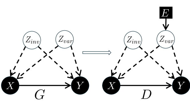
(Selection diagram): Let be a pair of SCMs relative to domain , sharing a causal diagram . is said to induce a selection diagram if is constructed as follows, a graphical illustration of the construction of the selection diagram is depicted in Figure 3:
1. Every edge in is also an edge in
2. contains an extra edge whenever there might exist a discrepancy or between and .
The set are denoted as selection variables.
Consider the scenario where we estimate a well-performed predictor in the domain , which can be seen as an estimation of the distribution . We are interested in assessing under which circumstance, the predictor can still accurately predict from in an arbitrary domain , i.e. accurately estimate the distribution . Achieving this criterion in prediction leads us to believe that the predictor demonstrates good generalization ability, and this criterion is often referred to as transportability.
Definition 4.2.
(Transportability): Let be a selection diagram relative to domain . Let be the pair of observational and interventional distributions of , and be the observational distribution of . The causal relation is said to be transportable from to in if is uniquely computable from in any model that induces .
If the causal mechanism satisfies the following theorem, then it is considered transportable.
Theorem 4.3.
(sufficient and necessary conditions of transportability (Pearl & Bareinboim, 2014)) The average causal effect is transportable from to if either one of the following conditions holds:
1. is trivially transportable.
2. There exists a set of covariates (possibly affected by ) such that is -admissible and for which is transportable.
3. There exists a set of covariates, that satisfy and for which is transportable.
The definition of trivially transportable is in Appendix A, and the definition of -admissible is as follows:
Definition 4.4.
(-admissibility). A set of variables satisfying in will be called S-admissible with respect to the causal effect of on . denote deleting all arrows pointing to node in .
If either one of the conditions of Theorem 4.3 is fulfilled, then it is possible to estimate , i.e. with our predictor. In the following, we are going to show, in Figure 2(a), unless the variables and are observable, the causal relation is not transportable.
Theorem 4.5.
The formulation of the causal mechanisms in Figure 2(a) can be written as (see Equation 15 in Appendix A for details). Where the is the invariance causal mechanism that doesn’t depend on the environment . However, without the observation of , the causal mechanism in Figure 2(a) is not transportable from to .
The detailed proof is provided in Appendix A. According to Theorem 4.5, is the invariant causal mechanism, that can be estimated from the source domain , while is the distribution of on target domain . We also provide a detailed analysis of the invariant causal mechanism in Appendix B. Theorem 4.5 state that estimating the target distribution required the observable of . In the next subsection, we provide a way to provably find (identify) these factors.
4.3 Methodology
According to Theorem 4.5, in order to capture the causal mechanism , access to is required. This challenge mirrors the well-established problem of definitively identifying the latent factors responsible for generating the data (Schölkopf et al., 2021; Hyvärinen & Oja, 2000). In the following subsection, we demonstrate that by leveraging interventional data, it is possible to identify these latent factors up to permutation and scaling. Building upon this insight, we propose CLIP-ICM to idenfify them.
We begin by considering the latent factor , sampled from the distribution supported on . The observed data is generated from through an injective mapping . The distribution of observed data is supported on . Our goal is to learn an encoder function , where represents its parameters. Ideally, the encoder function should invert the data-generating process, satisfying . However, due to the absence of additional knowledge about the latent distribution , we can only prove that, under a specific constraint, the encoder function’s output is a linear transformation of the true latent . Specifically, , where is an invertible matrix.
Proposition 4.6.
For an injective data generating process , suppose there exists an ideal encoder , such that . If for all environment , the encoder is trained optimal, and there exists a predictor for each environment, such that . Here, denote the classifier trained based on on environment , where denotes the parameters of this classifier. denote the classifier trained based on on environment , where denote the parameters of this classifier. Then the encoder identifies the latent factor up to an invertible linear transformation, i.e. .
The proof is illustrated in Appendix C. And Figure 4 provides a graphical explanation. This conclusion is a commonly recognized result from a series of works (Roeder et al., 2021; Ahuja et al., 2022b; Hyvarinen & Morioka, 2016; Zimmermann et al., 2022), and Proposition 4.6 provides a reproof of it in our scenario. CLIP can be considered satisfying Proposition 4.6 due to its impressive performance as a powerful pre-trained model. It was trained on a dataset of 400 million (image, text) pairs collected from the Internet and has demonstrated success in linear evaluation on downstream tasks (Radford et al., 2021). However, the linear identifiability of latent factors alone is insufficient to ensure the transportability of causal effects. This limitation arises from the fact that the mixing matrix is arbitrary, hindering the identification of domain-related factors .
Note that the aforementioned analyses are all based on observational data. The causal mechanism seeks to answer questions related to interventions, such as predicting the model’s response when changing a real-world image to a sketched painting. This involves intervening on factors like background color and texture. The operation, known as a -intervention, alters latent factors, and the resulting distribution of differs from the observational distribution . Formally, a -intervention sets the value of a specific latent factor to a fixed value , while the distribution of other latent factors is . The distribution of the interventional data is supported on .
Next, we demonstrate that by intervening on a specific latent factor, denoted as , such that for all , the -th output of the encoder remains a fixed value, the encoder can identify the corresponding intervened latent factor up to shift and scaling.
Theorem 4.7.
Consider observational data generated from an injective mapping , where the latent factors follow a distribution supported on . If a -intervention is applied to the latent factor , with the distribution of other latent factors denoted as , the resulting distribution of the interventional data is denoted as . Suppose that an encoder satisfies Proposition 4.6, and the output of the component of the encoder is required to take a fixed value for all . Then, the encoder identifies the intervened latent up to a shift and scaling, i.e., , where and .
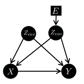
The proof is detailed in Appendix D. Theorem 4.7 presents an alternative approach for accessing and . When we intervene on all latent factors, the encoder identifies these factors up to permutation and scaling. This transformation alters the SCM from Figure 2(a) to Figure 2(b). As per Definition 4.4 and Theorem 4.3, the invariant factors is identified, this implies that the causal mechanism in Figure 2(b) is transportable. In other words, the encoder captures the invariant causal mechanism.
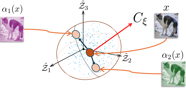
Theorem 4.7 provides a condition under which can be identified. Subsequently, leveraging the condition outlined in Theorem 4.7, we introduce a straightforward and efficient algorithm named CLIP-ICM. This algorithm functions as a post-processing step for the output of the CLIP encoders and is designed to meet the requirements of the condition specified in Theorem 4.7 We perform a set of interventions by utilizing data augmentation techniques, including color distortion, grayscale conversion, and Gaussian blur, on the raw image. Each type of data augmentation is regarded as an element of . For an image sample with different augmentations, it can be regarded that only the value of is changed while the remains a fixed value . Therefore, according to Theorem 4.7, we propose to estimate a linear transformation to produce the , where a total of augmentations are employed. Empirically, is the dimension of the estimated space, which is a hyper-parameter. We provide a detailed ablation study on this hyperparameter in Appendix I. The should exhibit two important characteristics: (1) the transformed representation should contain as much information about the original representation as possible. (2) should be invariant to any intervention on . Let , the objective for is:
|
|
(6) |
where is a hyperparameter, is the type of data augmentation, is the -th data augmentation and is the feature extractor.
Equation 6 can be viewed as a low-rank approximation problem (Golub et al., 1987) if we view the goal of finding a mapping from to through the lens of principle component analysis (Krogh & Hertz, 1991). We consider the true latent space of as a composite of two orthogonal subspaces, i.e. . According to Proposition 4.6, the learned representation space is an invertible linear transformation of the true latent space. Therefore, to find a mapping from to , is equivalent to finding the principle component of which is orthogonal to any intervention on , i.e. invariant to data augmentation. This is the idea of the second term in Equation 6. Empirically, we wish the invariant feature to contain as much information about the information of image as possible, and that is the idea of the first term in Equation 6.
To perform the invariant prediction, the invariant zero-shot prediction is obtained as follows:
|
|
(7) |
where the predictions are solely based on the similarities derived from . For the linear probe evaluation, the only applied to the output of the image encoder, and we train a classifier accordingly.
4.4 Generalization Analysis
In this subsection, we prove that the OOD generalization ability of our method is better than CLIP based on Rademacher complexity (Mohri et al., 2018), i.e., CLIP-ICM has a lower generalization bound compared to CLIP.
Let be the latent factors that generate observation data . According to Proposition 4.6, the output of the CLIP image encoder is , where is an invertible matrix. Assuming that the classification depends only on the invariant part, i.e. , we aim to learn a classifier based on the latent factor matrix . Under the above assumption, is a sparse matrix, while for the entangled latent factor matrix , the corresponding is dense.
For a hypothesis space and a data distribution , Rademacher complexity (Mohri et al., 2018) is a powerful metric to measure the OOD generalization ability of functions in . Denote by the OOD generalization error of hypothesis , our main conclusion could be summarized as follows:
Theorem 4.8.
For any data distribution , finite hypothesis spaces , the generalization error of hypothesis and hypothesis satisfies the following inequality:
| (8) |
Theorem 4.8 indicates that under identical confidence level, the OOD generalization error of is lower than , which ensures a better OOD generalization ability of CLIP-ICM. The proof is illustrated in Appendix E.
5 Experiment
| Algorithm | Backbone | C | L | S | V | Avg |
|---|---|---|---|---|---|---|
| ERM | R50 | 97.70.4 | 64.30.9 | 73.40.5 | 74.61.3 | 77.5 |
| IRM (Arjovsky et al., 2020) | R50 | 98.60.1 | 64.90.9 | 73.40.6 | 77.30.9 | 78.5 |
| GroupDRO (Sagawa* et al., 2019) | R50 | 97.30.3 | 63.40.9 | 69.50.8 | 76.70.7 | 76.7 |
| Mixup (Yan et al., 2020) | R50 | 98.30.6 | 64.81.0 | 72.10.5 | 74.30.8 | 77.4 |
| MMD (Li et al., 2018) | R50 | 97.70.1 | 64.01.1 | 72.80.2 | 75.33.3 | 77.5 |
| DANN (Ganin et al., 2016) | R50 | 99.00.3 | 65.11.4 | 73.10.3 | 77.20.6 | 78.6 |
| ARM (Zhang et al., 2021) | R50 | 98.70.2 | 63.60.7 | 71.31.2 | 76.70.6 | 77.6 |
| MBDG (Robey et al., 2021) | R50 | 98.3 | 68.1 | 68.8 | 76.3 | 77.9 |
| CLIP Linear-probe | R50 | 98.10.7 | 63.80.8 | 79.80.7 | 84.51.0 | 81.5 |
| CLIP-ICM Linear-probe | R50 | 99.20.1 | 69.90.3 | 80.50.3 | 89.50.9 | 84.8 |
| CLIPOOD (Shu et al., 2023) | ViT-B | 97.50.6 | 68.30.5 | 83.90.9 | 88.71.0 | 84.6 |
| CLIP Linear-probe | ViT-B | 93.70.2 | 65.40.2 | 76.40.2 | 79.10.3 | 78.7 |
| CLIP-ICM Linear-probe | ViT-B | 98.80.3 | 72.70.8 | 86.40.9 | 87.90.9 | 86.5 |
| CLIP Zero-shot | R50 | 99.20.0 | 69.50.0 | 69.80.0 | 84.90.0 | 80.9 |
| CLIP-ICM Zero-shot | R50 | 99.40.4 | 71.80.8 | 71.70.8 | 85.31.0 | 82.1 |
| CLIP Zero-shot | ViT-B | 99.90.0 | 70.10.0 | 73.50.0 | 86.10.0 | 82.4 |
| CLIP-ICM Zero-shot | ViT-B | 100.00.0 | 74.70.4 | 74.50.4 | 87.10.7 | 84.1 |
| Algorithm | Backbone | P | A | C | S | Avg |
|---|---|---|---|---|---|---|
| ERM | R50 | 97.20.3 | 84.70.4 | 80.80.6 | 79.31.0 | 85.5 |
| IRM (Arjovsky et al., 2020) | R50 | 96.70.6 | 84.81.3 | 76.41.1 | 76.11.0 | 83.5 |
| GroupDRO (Sagawa* et al., 2019) | R50 | 96.70.3 | 83.50.9 | 79.10.6 | 78.32.0 | 84.4 |
| Mixup (Yan et al., 2020) | R50 | 97.60.1 | 86.10.5 | 78.90.8 | 75.81.8 | 84.6 |
| MMD (Li et al., 2018) | R50 | 96.60.2 | 86.11.4 | 79.40.9 | 76.50.5 | 84.6 |
| DANN (Ganin et al., 2016) | R50 | 97.30.4 | 86.40.8 | 77.40.8 | 73.52.3 | 83.6 |
| ARM (Zhang et al., 2021) | R50 | 97.40.3 | 86.80.6 | 76.80.5 | 79.31.2 | 85.1 |
| MBDG (Robey et al., 2021) | R50 | 97.0 | 80.6 | 79.3 | 85.2 | 85.6 |
| CLIP Linear-probe | R50 | 99.20.7 | 91.70.8 | 92.50.7 | 82.30.2 | 91.4 |
| CLIP-ICM Linear-probe | R50 | 99.40.5 | 92.80.7 | 93.90.4 | 83.80.5 | 92.5 |
| CLIP Linear-probe | ViT-B | 97.30.7 | 98.40.1 | 99.50.4 | 90.40.3 | 96.4 |
| CLIP-ICM Linear-probe | ViT-B | 98.80.2 | 99.40.3 | 99.80.8 | 92.10.5 | 97.5 |
| CLIP Zero-shot | R50 | 99.30.0 | 91.00.0 | 93.10.0 | 80.50.0 | 91.0 |
| CLIP-ICM Zero-shot | R50 | 99.40.4 | 93.60.2 | 99.30.5 | 83.10.6 | 93.8 |
| CLIP Zero-shot | ViT-B | 100.00.0 | 97.40.0 | 99.20.0 | 88.10.0 | 96.1 |
| CLIP-ICM Zero-shot | ViT-B | 98.70.5 | 99.10.4 | 99.90.1 | 91.70.4 | 97.3 |
| Algorithm | Backbone | A | C | P | R | Avg |
|---|---|---|---|---|---|---|
| ERM | R50 | 61.30.7 | 52.40.3 | 75.80.1 | 76.60.3 | 66.5 |
| IRM (Arjovsky et al., 2020) | R50 | 58.92.3 | 52.21.6 | 72.12.9 | 74.02.5 | 64.3 |
| GroupDRO (Sagawa* et al., 2019) | R50 | 60.40.7 | 52.71.0 | 75.00.7 | 76.00.7 | 66.0 |
| Mixup (Yan et al., 2020) | R50 | 62.40.8 | 54.80.6 | 76.90.3 | 78.30.2 | 68.1 |
| MMD (Li et al., 2018) | R50 | 60.40.2 | 53.30.3 | 74.30.1 | 77.40.6 | 66.3 |
| DANN (Ganin et al., 2016) | R50 | 59.91.3 | 53.00.3 | 73.60.7 | 76.90.5 | 65.9 |
| ARM (Zhang et al., 2021) | R50 | 58.90.8 | 51.00.5 | 74.10.1 | 75.20.3 | 64.8 |
| SIG (Li et al., 2024) | R50 | 76.4 | 63.9 | 85.4 | 85.8 | 77.8 |
| CLIP Linear-probe | R50 | 68.00.8 | 46.30.3 | 80.40.9 | 81.90.7 | 69.1 |
| CLIP-ICM Linear-probe | R50 | 78.30.3 | 56.40.8 | 88.60.8 | 87.70.7 | 77.8 |
| CLIP Linear-probe | ViT-B | 78.90.9 | 69.30.9 | 90.30.3 | 89.00.2 | 81.9 |
| CLIP-ICM Linear-probe | ViT-B | 84.30.5 | 71.40.2 | 92.50.2 | 90.20.8 | 84.6 |
| CLIP Zero-shot | R50 | 71.30.0 | 50.40.0 | 81.70.0 | 82.60.0 | 71.5 |
| CLIP-ICM Zero-shot | R50 | 72.60.4 | 55.00.9 | 83.20.3 | 83.70.8 | 73.6 |
| CLIP Zero-shot | ViT-B | 83.30.0 | 65.30.0 | 89.00.0 | 89.30.0 | 81.7 |
| CLIP-ICM Zero-shot | ViT-B | 83.70.7 | 67.40.6 | 90.80.9 | 90.10.6 | 82.6 |
| Algorithm | Backbone | L100 | L38 | L43 | L46 | Avg |
|---|---|---|---|---|---|---|
| ERM | R50 | 49.84.4 | 42.11.4 | 56.91.8 | 35.73.9 | 46.1 |
| IRM (Arjovsky et al., 2020) | R50 | 54.61.3 | 39.81.9 | 56.21.8 | 39.60.8 | 47.6 |
| GroupDRO (Sagawa* et al., 2019) | R50 | 41.20.7 | 38.62.1 | 56.70.9 | 36.42.1 | 43.2 |
| Mixup (Yan et al., 2020) | R50 | 59.62.0 | 42.21.4 | 55.90.8 | 33.91.4 | 47.9 |
| MMD (Li et al., 2018) | R50 | 41.93.0 | 34.81.0 | 57.01.9 | 35.21.8 | 42.2 |
| DANN (Ganin et al., 2016) | R50 | 51.13.5 | 40.60.6 | 57.40.5 | 37.71.8 | 46.7 |
| ARM (Zhang et al., 2021) | R50 | 49.30.7 | 38.32.4 | 55.80.8 | 38.71.3 | 45.5 |
| CLIP Linear-probe | R50 | 52.01.0 | 34.40.6 | 56.10.9 | 32.80.2 | 44.1 |
| CLIP-ICM Linear-probe | R50 | 64.10.4 | 46.50.7 | 61.10.6 | 42.80.4 | 53.6 |
| CLIPOOD (Shu et al., 2023) | ViT-B | 74.60.3 | 57.30.5 | 59.10.9 | 47.70.9 | 59.7 |
| CLIP Linear-probe | ViT-B | 73.60.5 | 58.30.7 | 61.00.1 | 47.81.0 | 60.2 |
| CLIP-ICM Linear-probe | ViT-B | 78.70.5 | 60.20.9 | 66.00.8 | 52.40.1 | 64.3 |
| CLIP Zero-shot | R50 | 7.70.0 | 14.80.0 | 32.40.0 | 20.90.0 | 19.0 |
| CLIP-ICM Zero-shot | R50 | 38.80.4 | 33.60.6 | 33.60.1 | 30.10.7 | 34.0 |
| CLIP Zero-shot | ViT-B | 52.00.0 | 20.40.0 | 32.80.0 | 31.60.0 | 34.2 |
| CLIP-ICM Zero-shot | ViT-B | 59.30.4 | 46.20.4 | 52.40.7 | 41.60.8 | 49.9 |
| Algorithm | Backbone | CLIPART | INFOGRAPH | PAINTING | QUICKDRAW | REAL | SKETCH | Avg |
|---|---|---|---|---|---|---|---|---|
| ERM | R50 | 58.10.3 | 18.80.3 | 46.70.3 | 12.20.4 | 59.60.1 | 49.80.4 | 40.9 |
| IRM (Arjovsky et al., 2020) | R50 | 48.52.8 | 15.01.5 | 38.34.3 | 10.90.5 | 48.25.2 | 42.33.1 | 33.9 |
| GroupDRO (Sagawa* et al., 2019) | R50 | 47.20.5 | 17.50.4 | 33.80.5 | 9.30.3 | 51.60.4 | 40.10.6 | 33.3 |
| Mixup (Yan et al., 2020) | R50 | 55.70.3 | 18.50.5 | 44.30.5 | 12.50.4 | 55.80.3 | 48.20.5 | 39.2 |
| MMD (Li et al., 2018) | R50 | 32.113.3 | 11.04.6 | 26.811.3 | 8.72.1 | 32.713.8 | 28.911.9 | 23.4 |
| DANN (Ganin et al., 2016) | R50 | 53.10.2 | 18.30.1 | 44.20.7 | 11.80.1 | 55.50.4 | 46.80.6 | 38.3 |
| ARM (Zhang et al., 2021) | R50 | 49.70.3 | 16.30.5 | 40.91.1 | 9.40.1 | 53.40.4 | 43.50.4 | 35.5 |
| CLIP Linear-probe | R50 | 59.20.1 | 38.60.9 | 54.10.7 | 8.20.7 | 56.40.7 | 39.60.7 | 42.6 |
| CLIP-ICM Linear-probe | R50 | 63.10.1 | 50.10.2 | 66.21.0 | 19.70.3 | 83.80.4 | 63.20.3 | 57.8 |
| CLIPOOD (Shu et al., 2023) | ViT-B | 77.6 | 54.7 | 72.5 | 20.7 | 85.7 | 69.9 | 63.5 |
| CLIP Linear-probe | ViT-B | 73.90.5 | 40.20.5 | 62.10.2 | 15.10.3 | 76.90.1 | 62.00.7 | 55.0 |
| CLIP-ICM Linear-probe | ViT-B | 78.60.2 | 55.60.2 | 72.90.6 | 22.10.7 | 86.10.3 | 68.50.3 | 64.0 |
| CLIP Zero-shot | R50 | 53.10.0 | 39.20.0 | 52.90.0 | 5.70.0 | 76.70.0 | 48.00.0 | 45.9 |
| CLIP-ICM Zero-shot | R50 | 58.00.1 | 42.30.5 | 54.40.2 | 12.80.7 | 78.20.1 | 49.60.2 | 49.2 |
| CLIP Zero-shot | ViT-B | 70.20.0 | 46.60.0 | 65.00.0 | 13.70.0 | 82.90.0 | 62.70.0 | 56.8 |
| CLIP-ICM Zero-shot | ViT-B | 77.10.5 | 51.80.5 | 67.91.0 | 16.70.3 | 82.90.8 | 66.90.2 | 60.5 |
In this section, we first present the implementation details of our proposed CLIP-ICM, and present the classification results in the OOD datasets. Then, we conduct ablation studies of our proposed method. Experimental results demonstrate the effectiveness of our proposed method.
5.1 Implementation Details.
We employ 7 data augmentation techniques, i.e. ColorJitter, GrayScale, GaussianBlur, RandomInvert, RandomPosterize, RandomSolarize, and RandomEqualize for producing interventional data. The matrix is obtained by solving a low-rank approximation problem through singular value decomposition. For the linear-probe evaluation, the classifier undergoes training for a maximum of 1000 epochs with an penalty of implementing with the built-in function of Scikit-learn (Kramer, 2016). It is noteworthy that we learn in a totally unsupervised manner without the inclusion of label information. Additionally, during the estimating of , there are no images from the target domain included.
5.2 Classification in OOD datasets
Benchmarks and Evaluation Protocols.
To validate the effectiveness of the proposed CLIP-ICM in the OOD scenarios, we conduct experiments on the well-known benchmark DomainBed (Gulrajani & Lopez-Paz, 2020). Specifically, we select 5 datasets from DomainBed, namely VLCS (Fang et al., 2013), PCAS (Li et al., 2017), Office-Home(Venkateswara et al., 2017), TerraIncognita (Beery et al., 2018), and DomainNet (Peng et al., 2019). Each of these datasets contains the same categories across different domains. We utilize two types of evaluation protocols for our proposed CLIP-ICM, namely the zero-shot prediction and linear-probe prediction following (Radford et al., 2021). We follow the leave-one-out evaluation protocol, where one domain is chosen as the test domain and the other domains are chosen as the training domains.
Results.
The classification results of CLIP-ICM on VLCS, PCAS, Office-Home, TerraIncognita, and Domainnet are illustrated in Table 2, Table 3, Table 4, Table 5 and Table 6 respectively. It is clear from the tables that the CLIP-ICM significantly improves the performance of CLIP in both zero-shot and linear-probe manner. Specifically, in the linear probe of the VLCS dataset, CLIP-ICM shows a notable improvement of 10.0% in the S domain. Similarly, in the zero-shot setting of the TerraIncognita dataset, CLIP-ICM achieves an impressive improvement of 31.1% in the L100 domain. Moreover, the accuracy of CLIP-ICM is consistently improved across all domains, surpassing other state-of-the-art domain generalization methods.
5.3 Ablation Study
5.4 The impact of different data augmentation
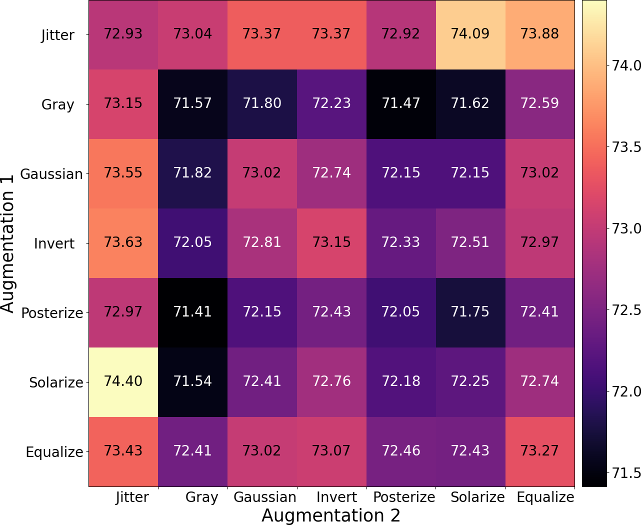
We investigate how CLIP-ICM performs with varying data augmentation strategies on the VLCS dataset. The experiments include different combinations of augmentation techniques and the zero-shot prediction accuracy on the LabelMe domain is illustrated in Figure 6. The diagonal of Figure 6 indicates scenarios where only one augmentation is applied, while other cells represent combinations of data augmentation techniques. It is noteworthy that the use of data augmentation significantly improves zero-shot performance, with certain combinations showing even more promising results.
5.5 The impact of hyperparameter .
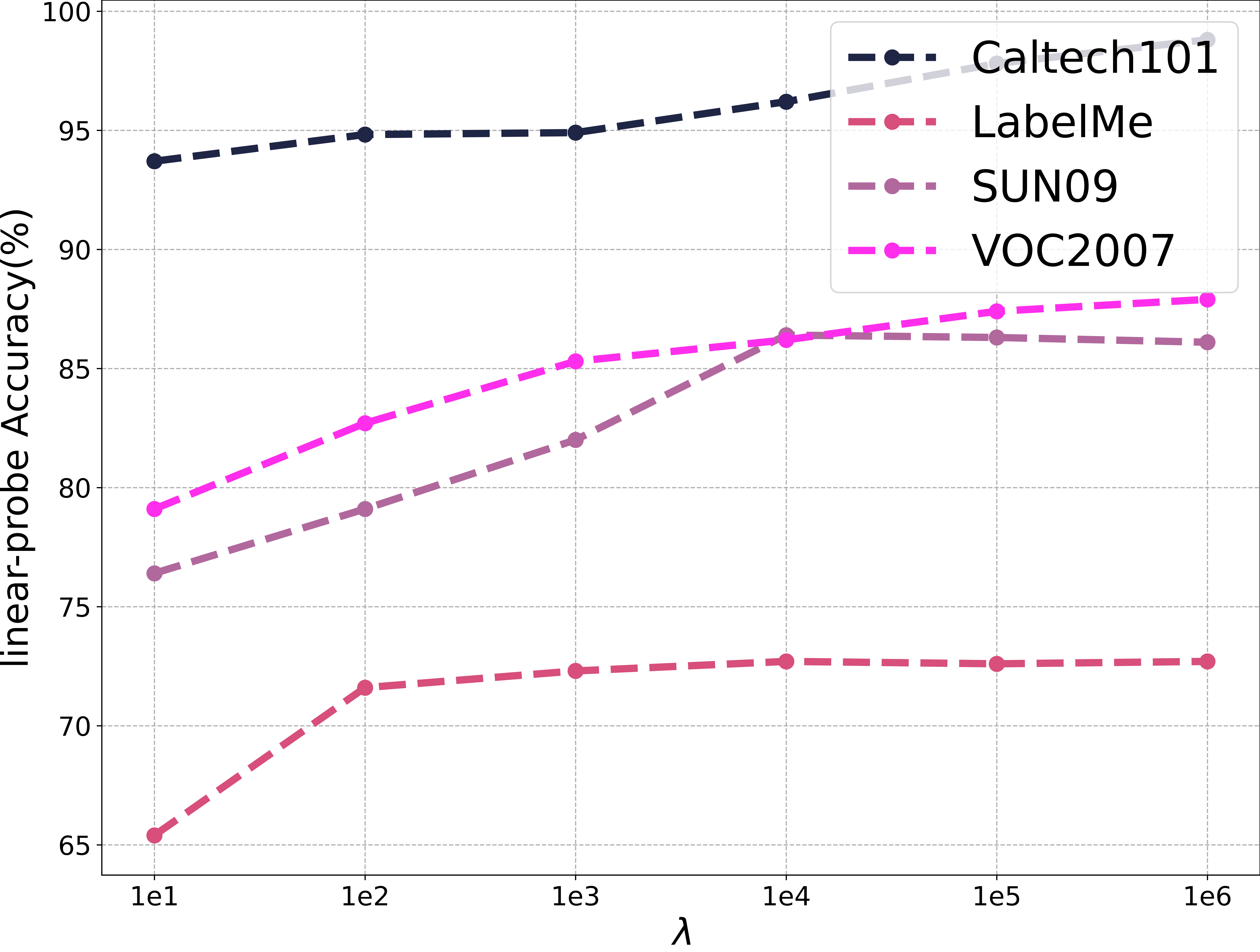
We conduct experiments on the VLCS dataset and visualize the results in Figure 7. From the results, we can observe that has a significant impact on the prediction results. This is because that higher value of indicates the second term of Equation 6 is more important and has a higher impact. These results illustrating the effectiveness of our proposed method.
6 Conclusion
In our work, we observe various performances of CLIP across different domains, noticing both well and unsatisfactory performance across domains. Through causal analysis, we demonstrate the inadequacy of the current CLIP model in capturing invariant causal mechanisms. Furthermore, we prove that the invariant causal mechanism is identifiable only when variant and invariant latent factors are identifiable. Consequently, we propose the CLIP-ICM methodology based on theoretical support derived from identifying latent factors with the aid of intervention data. Leveraging data augmentation, we incorporate a linear transformation onto the CLIP pre-trained model to acquire invariant latent factors. Theoretical evidence shows that our approach outperforms CLIP in OOD generalization. Experimental results demonstrate the superior results of CLIP-ICM on the Domainbed Benchmark in comparison to existing methods.
Impact Statements
We believe that this work is a step towards general artificial intelligence. This technique introduces the invariant causal mechanism into vision-language models, potentially revealing the physical world’s essence and promoting interpretable machine learning with significant societal implications.
References
- Abbe et al. (2023) Abbe, E., Bengio, S., Lotfi, A., and Rizk, K. Generalization on the Unseen, Logic Reasoning and Degree Curriculum. In Proceedings of the 40th International Conference on Machine Learning, pp. 31–60. PMLR, July 2023. ISSN: 2640-3498.
- Ahuja et al. (2020) Ahuja, K., Shanmugam, K., Varshney, K., and Dhurandhar, A. Invariant Risk Minimization Games. In Proceedings of the 37th International Conference on Machine Learning, pp. 145–155. PMLR, November 2020. ISSN: 2640-3498.
- Ahuja et al. (2022a) Ahuja, K., Caballero, E., Zhang, D., Gagnon-Audet, J.-C., Bengio, Y., Mitliagkas, I., and Rish, I. Invariance Principle Meets Information Bottleneck for Out-of-Distribution Generalization, November 2022a. arXiv:2106.06607 [cs, stat].
- Ahuja et al. (2022b) Ahuja, K., Mahajan, D., Syrgkanis, V., and Mitliagkas, I. Towards efficient representation identification in supervised learning, April 2022b. arXiv:2204.04606 [cs, stat].
- Ahuja et al. (2023) Ahuja, K., Mahajan, D., Wang, Y., and Bengio, Y. Interventional Causal Representation Learning. In Proceedings of the 40th International Conference on Machine Learning, pp. 372–407. PMLR, July 2023. ISSN: 2640-3498.
- Arjovsky et al. (2020) Arjovsky, M., Bottou, L., Gulrajani, I., and Lopez-Paz, D. Invariant Risk Minimization, March 2020. arXiv:1907.02893 [cs, stat].
- Bareinboim et al. (2022) Bareinboim, E., Correa, J. D., Ibeling, D., and Icard, T. On Pearl’s Hierarchy and the Foundations of Causal Inference. In Geffner, H., Dechter, R., and Halpern, J. Y. (eds.), Probabilistic and Causal Inference, pp. 507–556. ACM, New York, NY, USA, 1 edition, February 2022. ISBN 978-1-4503-9586-1. doi: 10.1145/3501714.3501743.
- Beery et al. (2018) Beery, S., Van Horn, G., and Perona, P. Recognition in terra incognita. In Proceedings of the European conference on computer vision (ECCV), pp. 456–473, 2018.
- Bengio et al. (2014) Bengio, Y., Courville, A., and Vincent, P. Representation Learning: A Review and New Perspectives, April 2014. arXiv:1206.5538 [cs].
- Bishop (1998) Bishop, C. M. Latent Variable Models. In Jordan, M. I. (ed.), Learning in Graphical Models, pp. 371–403. Springer Netherlands, Dordrecht, 1998. ISBN 978-94-010-6104-9 978-94-011-5014-9. doi: 10.1007/978-94-011-5014-9˙13.
- Buchholz et al. (2023) Buchholz, S., Rajendran, G., Rosenfeld, E., Aragam, B., Schölkopf, B., and Ravikumar, P. Learning Linear Causal Representations from Interventions under General Nonlinear Mixing, December 2023. arXiv:2306.02235 [cs, math, stat].
- Chen et al. (2020) Chen, T., Kornblith, S., Norouzi, M., and Hinton, G. A Simple Framework for Contrastive Learning of Visual Representations. In Proceedings of the 37th International Conference on Machine Learning, pp. 1597–1607. PMLR, November 2020. ISSN: 2640-3498.
- Chen et al. (2023) Chen, Y., Zhou, K., Bian, Y., Xie, B., Wu, B., Zhang, Y., Kaili, M., Yang, H., Zhao, P., Han, B., and Cheng, J. Pareto Invariant Risk Minimization: Towards Mitigating the Optimization Dilemma in Out-of-Distribution Generalization. February 2023.
- Daunhawer et al. (2023) Daunhawer, I., Bizeul, A., Palumbo, E., Marx, A., and Vogt, J. E. Identifiability Results for Multimodal Contrastive Learning, March 2023. arXiv:2303.09166 [cs, stat].
- Elhoseiny et al. (2013) Elhoseiny, M., Saleh, B., and Elgammal, A. Write a classifier: Zero-shot learning using purely textual descriptions. In Proceedings of the IEEE International Conference on Computer Vision, pp. 2584–2591, 2013.
- Fang et al. (2013) Fang, C., Xu, Y., and Rockmore, D. N. Unbiased metric learning: On the utilization of multiple datasets and web images for softening bias. In Proceedings of the IEEE International Conference on Computer Vision, pp. 1657–1664, 2013.
- Frome et al. (2013) Frome, A., Corrado, G. S., Shlens, J., Bengio, S., Dean, J., Ranzato, M., and Mikolov, T. Devise: A deep visual-semantic embedding model. Advances in neural information processing systems, 26, 2013.
- Ganin et al. (2016) Ganin, Y., Ustinova, E., Ajakan, H., Germain, P., Larochelle, H., Laviolette, F., March, M., and Lempitsky, V. Domain-adversarial training of neural networks. Journal of machine learning research, 17(59):1–35, 2016.
- Gao et al. (2023) Gao, P., Geng, S., Zhang, R., Ma, T., Fang, R., Zhang, Y., Li, H., and Qiao, Y. CLIP-Adapter: Better Vision-Language Models with Feature Adapters. International Journal of Computer Vision, September 2023. ISSN 0920-5691, 1573-1405. doi: 10.1007/s11263-023-01891-x.
- Glymour et al. (2016) Glymour, M., Pearl, J., and Jewell, N. P. Causal Inference in Statistics: A Primer. John Wiley & Sons, January 2016. ISBN 978-1-119-18686-1. Google-Books-ID: I0V2CwAAQBAJ.
- Golub et al. (1987) Golub, G. H., Hoffman, A., and Stewart, G. W. A generalization of the Eckart-Young-Mirsky matrix approximation theorem. Linear Algebra and its applications, 88:317–327, 1987. doi: 10.1016/0024-3795(87)90114-5. Publisher: Elsevier.
- Gulrajani & Lopez-Paz (2020) Gulrajani, I. and Lopez-Paz, D. In Search of Lost Domain Generalization, July 2020. arXiv:2007.01434 [cs, stat].
- He et al. (2022) He, K., Chen, X., Xie, S., Li, Y., Dollár, P., and Girshick, R. Masked autoencoders are scalable vision learners. In Proceedings of the IEEE/CVF conference on computer vision and pattern recognition, pp. 16000–16009, 2022.
- Hendrycks & Dietterich (2019) Hendrycks, D. and Dietterich, T. Benchmarking Neural Network Robustness to Common Corruptions and Perturbations, March 2019. arXiv:1903.12261 [cs, stat].
- Hyvarinen & Morioka (2016) Hyvarinen, A. and Morioka, H. Unsupervised feature extraction by time-contrastive learning and nonlinear ica. Advances in neural information processing systems, 29, 2016.
- Hyvarinen & Morioka (2017) Hyvarinen, A. and Morioka, H. Nonlinear ICA of Temporally Dependent Stationary Sources. In Proceedings of the 20th International Conference on Artificial Intelligence and Statistics, pp. 460–469. PMLR, April 2017. ISSN: 2640-3498.
- Hyvärinen & Oja (2000) Hyvärinen, A. and Oja, E. Independent component analysis: algorithms and applications. Neural Networks, 13(4):411–430, June 2000. ISSN 0893-6080. doi: 10.1016/S0893-6080(00)00026-5.
- Hyvärinen & Pajunen (1999) Hyvärinen, A. and Pajunen, P. Nonlinear independent component analysis: Existence and uniqueness results. Neural Networks, 12(3):429–439, April 1999. ISSN 0893-6080. doi: 10.1016/S0893-6080(98)00140-3.
- Jia et al. (2021) Jia, C., Yang, Y., Xia, Y., Chen, Y.-T., Parekh, Z., Pham, H., Le, Q., Sung, Y.-H., Li, Z., and Duerig, T. Scaling up visual and vision-language representation learning with noisy text supervision. In International conference on machine learning, pp. 4904–4916. PMLR, 2021.
- Kingma & Welling (2013) Kingma, D. P. and Welling, M. Auto-encoding variational bayes. arXiv preprint arXiv:1312.6114, 2013.
- Kramer (2016) Kramer, O. Scikit-Learn. In Machine Learning for Evolution Strategies, volume 20, pp. 45–53. Springer International Publishing, Cham, 2016. ISBN 978-3-319-33381-6 978-3-319-33383-0. doi: 10.1007/978-3-319-33383-0˙5. Series Title: Studies in Big Data.
- Krogh & Hertz (1991) Krogh, A. and Hertz, J. A simple weight decay can improve generalization. Advances in neural information processing systems, 4, 1991.
- Kügelgen et al. (2021) Kügelgen, J. V., Sharma, Y., Gresele, L., Brendel, W., Schölkopf, B., Besserve, M., and Locatello, F. Self-Supervised Learning with Data Augmentations Provably Isolates Content from Style. November 2021.
- Lachapelle et al. (2022) Lachapelle, S., López, P. R., Sharma, Y., Everett, K., Priol, R. L., Lacoste, A., and Lacoste-Julien, S. Disentanglement via Mechanism Sparsity Regularization: A New Principle for Nonlinear ICA, February 2022. arXiv:2107.10098 [cs, stat].
- Li et al. (2017) Li, D., Yang, Y., Song, Y.-Z., and Hospedales, T. M. Deeper, broader and artier domain generalization. In Proceedings of the IEEE international conference on computer vision, pp. 5542–5550, 2017.
- Li et al. (2018) Li, H., Pan, S. J., Wang, S., and Kot, A. C. Domain generalization with adversarial feature learning. In Proceedings of the IEEE conference on computer vision and pattern recognition, pp. 5400–5409, 2018.
- Li et al. (2024) Li, Z., Cai, R., Chen, G., Sun, B., Hao, Z., and Zhang, K. Subspace identification for multi-source domain adaptation. Advances in Neural Information Processing Systems, 36, 2024.
- Locatello et al. (2019) Locatello, F., Bauer, S., Lucic, M., Rätsch, G., Gelly, S., Schölkopf, B., and Bachem, O. Challenging Common Assumptions in the Unsupervised Learning of Disentangled Representations, June 2019. arXiv:1811.12359 [cs, stat].
- Locatello et al. (2020) Locatello, F., Poole, B., Rätsch, G., Schölkopf, B., Bachem, O., and Tschannen, M. Weakly-supervised disentanglement without compromises. In International Conference on Machine Learning, pp. 6348–6359. PMLR, 2020.
- Miller et al. (2021) Miller, J. P., Taori, R., Raghunathan, A., Sagawa, S., Koh, P. W., Shankar, V., Liang, P., Carmon, Y., and Schmidt, L. Accuracy on the line: on the strong correlation between out-of-distribution and in-distribution generalization. In International Conference on Machine Learning, pp. 7721–7735. PMLR, 2021.
- Mohri et al. (2018) Mohri, M., Rostamizadeh, A., and Talwalkar, A. Foundations of machine learning. MIT press, 2018.
- Norouzi et al. (2014) Norouzi, M., Mikolov, T., Bengio, S., Singer, Y., Shlens, J., Frome, A., Corrado, G. S., and Dean, J. Zero-Shot Learning by Convex Combination of Semantic Embeddings, March 2014. arXiv:1312.5650 [cs].
- Oord et al. (2019) Oord, A. v. d., Li, Y., and Vinyals, O. Representation Learning with Contrastive Predictive Coding, January 2019. arXiv:1807.03748 [cs, stat].
- Pearl (2009) Pearl, J. Causality. Cambridge university press, 2009.
- Pearl & Bareinboim (2014) Pearl, J. and Bareinboim, E. External Validity: From Do-Calculus to Transportability Across Populations. Statistical Science, 29(4):579–595, November 2014. ISSN 0883-4237, 2168-8745. doi: 10.1214/14-STS486. Publisher: Institute of Mathematical Statistics.
- Peng et al. (2019) Peng, X., Bai, Q., Xia, X., Huang, Z., Saenko, K., and Wang, B. Moment matching for multi-source domain adaptation. In Proceedings of the IEEE/CVF international conference on computer vision, pp. 1406–1415, 2019.
- Peters et al. (2015) Peters, J., Bühlmann, P., and Meinshausen, N. Causal inference using invariant prediction: identification and confidence intervals, November 2015. arXiv:1501.01332 [stat].
- Peters et al. (2016) Peters, J., Bühlmann, P., and Meinshausen, N. Causal Inference by using Invariant Prediction: Identification and Confidence Intervals. Journal of the Royal Statistical Society Series B: Statistical Methodology, 78(5):947–1012, November 2016. ISSN 1369-7412, 1467-9868. doi: 10.1111/rssb.12167.
- Pham et al. (2023) Pham, H., Dai, Z., Ghiasi, G., Kawaguchi, K., Liu, H., Yu, A. W., Yu, J., Chen, Y.-T., Luong, M.-T., Wu, Y., Tan, M., and Le, Q. V. Combined scaling for zero-shot transfer learning. Neurocomputing, 555:126658, October 2023. ISSN 09252312. doi: 10.1016/j.neucom.2023.126658.
- Radford et al. (2021) Radford, A., Kim, J. W., Hallacy, C., Ramesh, A., Goh, G., Agarwal, S., Sastry, G., Askell, A., Mishkin, P., Clark, J., Krueger, G., and Sutskever, I. Learning Transferable Visual Models From Natural Language Supervision. In Proceedings of the 38th International Conference on Machine Learning, pp. 8748–8763. PMLR, July 2021. ISSN: 2640-3498.
- Robey et al. (2021) Robey, A., Pappas, G. J., and Hassani, H. Model-based domain generalization. Advances in Neural Information Processing Systems, 34:20210–20229, 2021.
- Roeder et al. (2021) Roeder, G., Metz, L., and Kingma, D. On linear identifiability of learned representations. In International Conference on Machine Learning, pp. 9030–9039. PMLR, 2021.
- Sagawa* et al. (2019) Sagawa*, S., Koh*, P. W., Hashimoto, T. B., and Liang, P. Distributionally Robust Neural Networks. December 2019.
- Schoelkopf et al. (2012) Schoelkopf, B., Janzing, D., Peters, J., Sgouritsa, E., Zhang, K., and Mooij, J. On Causal and Anticausal Learning, June 2012. arXiv:1206.6471 [cs, stat].
- Schölkopf et al. (2021) Schölkopf, B., Locatello, F., Bauer, S., Ke, N. R., Kalchbrenner, N., Goyal, A., and Bengio, Y. Toward Causal Representation Learning. Proceedings of the IEEE, 109(5):612–634, May 2021. ISSN 1558-2256. doi: 10.1109/JPROC.2021.3058954. Conference Name: Proceedings of the IEEE.
- Shu et al. (2023) Shu, Y., Guo, X., Wu, J., Wang, X., Wang, J., and Long, M. CLIPood: Generalizing CLIP to Out-of-Distributions, July 2023. arXiv:2302.00864 [cs].
- Socher et al. (2013) Socher, R., Ganjoo, M., Manning, C. D., and Ng, A. Zero-shot learning through cross-modal transfer. Advances in neural information processing systems, 26, 2013.
- Squires et al. (2023) Squires, C., Seigal, A., Bhate, S. S., and Uhler, C. Linear causal disentanglement via interventions. In International Conference on Machine Learning, pp. 32540–32560. PMLR, 2023.
- Suter et al. (2019) Suter, R., Miladinovic, D., Schölkopf, B., and Bauer, S. Robustly disentangled causal mechanisms: Validating deep representations for interventional robustness. In International Conference on Machine Learning, pp. 6056–6065. PMLR, 2019.
- Taori et al. (2020) Taori, R., Dave, A., Shankar, V., Carlini, N., Recht, B., and Schmidt, L. Measuring robustness to natural distribution shifts in image classification. Advances in Neural Information Processing Systems, 33:18583–18599, 2020.
- Torralba & Efros (2011) Torralba, A. and Efros, A. A. Unbiased look at dataset bias. In CVPR 2011, pp. 1521–1528, Colorado Springs, CO, USA, June 2011. IEEE. ISBN 978-1-4577-0394-2. doi: 10.1109/CVPR.2011.5995347.
- Venkateswara et al. (2017) Venkateswara, H., Eusebio, J., Chakraborty, S., and Panchanathan, S. Deep hashing network for unsupervised domain adaptation. In Proceedings of the IEEE conference on computer vision and pattern recognition, pp. 5018–5027, 2017.
- Wald et al. (2021) Wald, Y., Feder, A., Greenfeld, D., and Shalit, U. On Calibration and Out-of-Domain Generalization. In Advances in Neural Information Processing Systems, volume 34, pp. 2215–2227. Curran Associates, Inc., 2021.
- Yan et al. (2020) Yan, S., Song, H., Li, N., Zou, L., and Ren, L. Improve unsupervised domain adaptation with mixup training. arXiv preprint arXiv:2001.00677, 2020.
- Zhang et al. (2021) Zhang, M., Marklund, H., Dhawan, N., Gupta, A., Levine, S., and Finn, C. Adaptive risk minimization: Learning to adapt to domain shift. Advances in Neural Information Processing Systems, 34:23664–23678, 2021.
- Zhang et al. (2022) Zhang, X., Gu, S. S., Matsuo, Y., and Iwasawa, Y. Domain Prompt Learning for Efficiently Adapting CLIP to Unseen Domains, August 2022. arXiv:2111.12853 [cs].
- Zhou et al. (2022a) Zhou, K., Yang, J., Loy, C. C., and Liu, Z. Conditional Prompt Learning for Vision-Language Models, October 2022a. arXiv:2203.05557 [cs].
- Zhou et al. (2022b) Zhou, K., Yang, J., Loy, C. C., and Liu, Z. Learning to Prompt for Vision-Language Models. International Journal of Computer Vision, 130(9):2337–2348, September 2022b. ISSN 0920-5691, 1573-1405. doi: 10.1007/s11263-022-01653-1. arXiv:2109.01134 [cs].
- Zimmermann et al. (2022) Zimmermann, R. S., Sharma, Y., Schneider, S., Bethge, M., and Brendel, W. Contrastive Learning Inverts the Data Generating Process, April 2022. arXiv:2102.08850 [cs].
Appendix
This supplementary material provides detailed proofs for the theorem and proposition mentioned in the main text. Furthermore, additional experimental results and the implementation detailed are provided.
-
•
Appendix A provides the proof of Theorem 4.5 in the main text.
-
•
Appendix D provides the proof of Theorem 4.7 in the main text.
-
•
Appendix C provides the proof of Proposition 4.6 in the main text.
-
•
Appendix E provides the proof of Theorem 4.8 in the main text.
-
•
Section E.1 provides the pseudo code for CLIP-ICM.
-
•
Appendix F provides detailed description of the used datasets.
Appendix A Proof for Theorem 4.5
Before we proceed to the proof of Theorem 4.5, we first provide some basic definitions of causal inference.
Definition A.1.
(-separation): A set of nodes is said to block a path if either
1. contains at least one arrow-emitting node that is in ,
2. contains at least one collision node that is outside and has no descendant in .
If blocks all paths from set to set , it is said to -separate and . and are independent given , written .
The -separation reflects the conditional independencies that hold the distribution that is compatible with the DAG.
Definition A.2.
(Rules of do-calculus) Let be arbitrary disjoint sets of nodes in a causal DAG . We denote by the graph obtained by deleting from all arrows pointing to nodes in . Likewise, we denote by the graph obtained by deleting from all arrows emerging from nodes in . The notation represents the deletion of both incoming and outgoing arrows.
1. Insertion/deletion of observations.
2. Action/observation exchange.
3. Insertion/deletion of actions.
where is the set of -nodes that are not ancestors of any -node in .
Definition A.3.
(Identifiability) A causal query is identifiable, given a set of assumptions , if for any two (fully specified) models, and that satisfy , we have:
Definition A.4.
(Trivial transportability). A causal relation is said to be trivially transportable from to , if is identifiable from .
is trivially transportable if we can directly estimate from observational data of , unaided by the causal information from . The following state the sufficient and necessary conditions of transportability of average causal effect .
Theorem A.5.
(sufficient and necessary conditions of transportability (Pearl & Bareinboim, 2014)) The average causal effect is transportable from to if either one of the following conditions holds:
1. is trivially transportable.
2. There exists a set of covariates (possibly affected by ) such that is -admissible and for which is transportable.
3. There exists a set of covariates, that satisfy and for which is transportable.
Proof.
1. According to Definition A.4, the causal relationship can be directly estimated from observational data of .
2. If condition 2 holds, it implies:
| (9) | ||||
The transportability of reduces to a star-free expression and therefore is transportable. 3. If condition 3 holds, it implies:
| (10) | ||||
According to Rule 3 of Definition A.2, the transportability of would render to a star-free expression and render transportable. This ends the proof. ∎
We are now prepared to present the proof for Theorem 4.5 in the main text:
Theorem A.6.
The formulation of the causal mechanisms in Figure 2(a) can be written as (see Equation 15 in Appendix A for details). Where the is the invariance causal mechanism that doesn’t depend on the environment . However, without the observation of and , the causal mechanism in Figure 2(a) is not transportable from to .
Proof.
Suppose that the causal mechanism in Figure 2(a) is transportable from to , we aim to prove our conclusion by reduction to absurdity. The causal mechanism we would like to estimate is:
| (11) | ||||
From the Rule 1 of Definition A.2, we have
| (12) |
because satisfies in . Therefore, according to Definition 4.4, the -admissible with respect to the causal effect of on . According to Definition A.1, is a collision node, then:
| (13) |
and similarly for and :
| (14) |
Therefore, the Equation 11 can be rewrite as:
| (15) |
However, in Figure 2(a), the and is unobservable, making the causal effect non-transportable. This ends the proof. ∎
Appendix B Further analysis on the invariant causal mechanism
To give a more comprehensive understanding of the invariant causal mechanism, we further provide a detailed analysis as follows: From Equation 15, the distribution of latent variable is invariant across domains, while the distribution of is dependent on the environment.
Without loss of generality, let , , the prediction of CLIP can be written as:
| (16) | ||||
| (17) |
if we divide both above and below:
| (18) |
And , where is the angle between and . Therefore:
| (19) |
According to Hölder’s inequality:
| (20) |
Without loss of generality, suppose is a constant, . Then the following inequality holds:
| (21) | ||||
| (22) |
Theoretically, maximizing the RHS of the above inequality is a sufficient condition for maximizing the LHS, which is the prediction of CLIP. While the RHS is the invariant prediction of Equation 6 of the original paper, i.e. the invariant causal mechanism.
Empirically, the text prompts are fixed across different domains, e.g. ”A photo of [cls]”. Therefore, the is fixed across different domains, while is the variance part of image embedding and changes across domains. To make an invariant prediction, the part of the embedding of prompt of each class should be the same, , therefore, . The invariant prediction can be written as:
| (23) |
Appendix C Proof for Proposition 4.6
Building upon prior works (Roeder et al., 2021; Ahuja et al., 2022b; Hyvarinen & Morioka, 2016; Zimmermann et al., 2022), we offer proof demonstrating that CLIP identifies latent factors up to an invertible linear transformation, and we also reuse some of their proof techniques.
Proposition C.1.
For an injective data generating process , suppose there exists an ideal encoder , such that . If for all environment , the encoder is trained optimal, and there exists a predictor for each environment, such that . Then the encoder identifies the latent factor up to an invertible linear transformation, i.e. .
Proof.
We proceed by constructing the invertible linear transformations to satisfy , where is an invertible matrix. First, we assume that for any for which it holds that , and for any given , we assume that by repeated sampling class from the observation data and picking , we can construct a set of distinct tuples , such that the matrices and are invertible, where consists of columns and consists of columns . The likelihood ratios for these points are equal:
| (24) |
Substituting our model definition from Equation 3, we find:
| (25) |
Taking the logarithm of both sides, this simplifies to:
| (26) |
By repeating Equation 26 times and by the diversity condition noted above, the resulting difference vectors are linearly independent. We collect these vectors together as the columns of -dimensional matrices and , forming the following system of linear equations:
| (27) |
Therefore, where is invertible. ∎
Appendix D Proof for Theorem 4.7
Theorem D.1.
Consider observational data generated from an injective mapping , where the latent factors follow a distribution supported on . If a -intervention is applied to the latent factor , with the distribution of other latent factors denoted as , the resulting distribution of the interventional data is denoted as . Suppose that an encoder satisfies Proposition 4.6, and the output of the component of the encoder is required to take a fixed value for all . Then, the encoder identifies the intervened latent up to a shift and scaling, i.e., , where and .
Proof.
The encoder satisfies Proposition 4.6 implies that . The -th element of . Considering the support of the distribution of the unintervened latent is a non-empty subset. We separately write the intervened latent as , where is the intervened latent and is the set of other latent factors other than . Then, can be written as:
| (28) |
where represents the -th element of the -th row, and denotes the -th row excluding the -th element. If the output of the -th component of the encoder to have a fixed value of , then setting yields the following:
| (29) |
Consider another data point from the interventional distribution . We can express as . The is nearly identical to , except for , which is obtained by adding to . Here, is a small positive value, and represents a one-hot vector with the -th element as one and the others as zero.
| (30) |
If we use Equation 29 minus Equation 30, the results are as followed:
| (31) | ||||
This implies the -th element in is zero. Iterative apply to the can proof that is zero, which makes . This ends the proof. ∎
Appendix E Proof for Theorem 4.8
Before we proceed to the proof of Theorem 4.8, we first give the generalization bound theorem in (Mohri et al., 2018) and illustrate Massart’s lemma, i.e. Lemma E.2.
Theorem E.1.
Given the data distribution , then for any hypothesis in the finite set and , with probability at least , it holds that:
| (32) |
where represents Rademacher complexity.
Lemma E.2.
Let be a finite set, with , then the following holds:
| (33) |
where s are independent uniform random variables taking values in and are the components of vector .
Proof.
The result follows immediately from the bound on the expectation of a maximum given by Corollary D.11 from (Mohri et al., 2018) since the random variables are independent and each takes values in with . ∎
Note that the left side of Equation 33 is the formulation of Rademacher complexity, Lemma E.2 provides an upper bound of Rademacher complexity for arbitrary space. Using this result, we can now demonstrate Theorem 4.8.
Theorem E.3.
For any data distribution , hypothesis spaces , the generalization error of hypothesis and hypothesis satisfies the following inequality:
| (34) |
Proof.
Due to the causality-based identification process of our method, the dimension of hypothesis space and satisfies inequality:
| (35) |
Further, the upper bound of Rademacher complexity of hypothesis space and satisfies:
| (36) |
The result indicates that the Rademacher complexity satisfies:
| (37) |
According to (Mohri et al., 2018), the upper bound of generalization error satisfies Theorem E.1. For the generalization bound of CLIP-ICM and CLIP only differs in the Rademacher complexity item, we can dedicate from the above illustration that CLIP-ICM has a lower generalization bound than CLIP:
| (38) |
The above result indicates that the OOD generalization ability of our proposed method is better compared with CLIP. This ends our proof. ∎
E.1 Pseudo Code
The pseodo code of CLIP-ICM is illustrated in Algorithm 1.
Appendix F Dataset Details
DOMAINBED includes downloaders and loaders for seven multi-domain image classification tasks:
-
•
PACS (Li et al., 2017) comprises four domains . This dataset contains 9,991 examples of dimension (3, 224, 224) and 7 classes.
-
•
VLCS (Fang et al., 2013) comprises photographic domains . This dataset contains 10,729 examples of dimension (3, 224, 224) and 5 classes.
-
•
Office-Home (Venkateswara et al., 2017) includes domains . This dataset contains 15,588 examples of dimension (3, 224, 224) and 65 classes.
-
•
Terra Incognita (Beery et al., 2018) contains photographs of wild animals taken by camera traps at locations . Our version of this dataset contains 24,788 examples of dimension (3, 224, 224) and 10 classes.
-
•
DomainNet (Peng et al., 2019) has six domains . This dataset contains 586,575 examples of size (3, 224, 224) and 345 classes.
For all datasets, we first pool the raw training, validation, and testing images together. For each random seed, we then instantiate random training, validation, and testing splits.
Appendix G Experiments on ImageNet-C
To evaluate the robustness of our proposed CLIP-ICM, we also conduct experiments on the corruption-based dataset ImageNet-C (Hendrycks & Dietterich, 2019). ImageNet-C is an open-source dataset that consists of algorithmically generated corruptions (blur, noise) applied to the ImageNet test set. We report the mean Corruption Error (mCE) to evaluate the robustness of our method. In addition to the mCE metric, we have also compared the clean error rates. Our comparative analysis includes the evaluation of a ResNet50 baseline, CLIP Linear-probe, and CLIP-ICM Linear-probe. It is noteworthy that all these methods utilize the ResNet50 architecture as their backbone network.
| Algorithm | mCE | Clean Error |
|---|---|---|
| ResNet-50 Baseline | 76.7% | 23.85% |
| CLIP Linear-probe | 62.92% | 26.70% |
| CLIP-ICM Linear-probe | 51.74% | 22.67% |
From Table 7, it is clear that our method achieves superior performance on the ImageNet-C dataset compared to the ResNet-50 Baseline. Additionally, it shows an improvement in performance on the original ImageNet dataset as well.
Appendix H More comparison with related works
H.1 Model-based Domain Generalization (Robey et al., 2021)
Model-based Domain Generalization (Robey et al., 2021) also also proposes an SCM, their analysis method is different from ours. They believe that in domain shift, an instance is generated by an underlying random variable and jointly passing through a domain-transfer model . In our causal diagram analysis, we believe that the sample is generated by and jointly.
MBDG obtains the invariant features by utilizing a pre-trained domain-transfer model to constrain the distance between the features extracted by the feature extractor and the representations generated by the domain-transfer model.
H.2 On Calibration and Out-of-domain Generalization (Wald et al., 2021)
From the perspective of SCM analysis, (Wald et al., 2021) proposes a causal graph that categorizes features into , , and . This categorization is based on the understanding that certain variables have a direct causal influence on the outcome . In contrast, our proposed causal graph incorporates the environmental variable as an indirect causal pathway to .
From the methodological standpoint, the article addresses the OOD problem by proposing the need to find a classifier such that , which implies that the classifier is calibrated. Similar to IRM, the article introduces a loss function called CLOvE designed to constrain classifiers across different domains to produce consistent results. Our approach, however, does not require modifications to the backbone model, nor do we necessitate the training of additional classifiers. Instead, we achieve a zero-shot classifier that remains invariant across each domain.
H.3 Subspace Identification Guarantee (Li et al., 2024)
From the perspective of SCM analysis, SIG views the data generation process through 4 kinds of latent factors. In our SCM, can be regarded as a domain-invariant variable, and can be regarded as a domain-variant variable. Since in our causal diagram, represents the description of the picture, therefore, we do not distinguish between label-irrelevant and label-relevant variables in our modeling.
From a methodological perspective, SIG uses an end-to-end, reconstruction-based network, while we use a pre-trained CLIP backbone network. SIG uses a variation-inference method to identify latent factors, while we use an intervention method to identify latent factors.
A comparative analysis is presented to illustrate the performance of our method alongside the SIG’s approach to the Office-Home dataset. Both our method and the SIG’s method utilize the ResNet50 architecture as the backbone network. Similarly, the performance on the DomainNet dataset is compared, with both our method and the SIG’s method employing the ResNet101 backbone network.
H.4 Domain Prompt Learning (Zhang et al., 2022)
(Zhang et al., 2022) introduces Domain Prompt Learning (DPL), a novel approach that improves the domain generalization performance of the CLIP model on various datasets by generating conditional prompts, achieving higher accuracy without fine-tuning the entire model. Compared with our method, also includes training a fully connected network with label information in the objective function. We provide the comparison results below:
| Method | VLCS | PACS | OfficeHome | Terra | Avg |
|---|---|---|---|---|---|
| CLIP Linear-Probe | 78.7 | 96.4 | 81.9 | 60.2 | 79.3 |
| CLIP + DPL (Zhang et al., 2022) | 84.3 | 97.3 | 84.2 | 52.6 | 79.6 |
| CLIP-ICM Linear-Probe | 86.5 | 97.5 | 84.6 | 64.3 | 83.2 |
H.5 Self-Supervised Learning with Data Augmentations Provably Isolates Content from Style (Kügelgen et al., 2021)
(Kügelgen et al., 2021) also interpret data augmentations as counterfactuals, and use them to obtain the invariant factors. Our work differs from theirs in three key aspects: the background setting, the research problem, and the implementation method.
Firstly, the problem studied by (Kügelgen et al., 2021) is set within the framework of self-supervised contrastive learning. In their paper, the term ”invariant factor” refers to the invariant parts derived from two different augmented perspectives within a positive sample pair. In contrast, the ”invariant factor” in our paper refers to the latent factors that remain unchanged across different domains. Due to the diversity of augmentation methods employed in self-supervision (Chen et al., 2020), the invariant factors they investigate do not align with the invariant factors we examine.
Secondly, in their paper, they consider an in-distribution problem, where all representations belong to the same distribution , and they do not take into account the different distributions across various domains. In our paper, however, we investigate an out-of-distribution problem. We posit that the distribution of is influenced by the environment, meaning that .
Lastly, their experiments are solely based on analyzing the capabilities of SimCLR to identify latent factors, without proposing any new methods. In contrast, based on our theoretical analysis, we proposed a novel method for identifying invariant representations.
| Algorithm | Backbone | Clipart | Infograph | Painting | Quickdraw | Real | Sketch | Avg |
|---|---|---|---|---|---|---|---|---|
| SIG (Li et al., 2024) | R101 | 72.7 | 32.0 | 61.5 | 20.5 | 72.4 | 59.5 | 53.0 |
| CLIP-ICM Linear-probe | R101 | 73.6 | 38.2 | 69.4 | 19.2 | 74.1 | 65.5 | 56.6 |
Appendix I Ablation study on dimension of
As we mentioned at Section 4.3, the dimension of is a hyperparameter. To investigate the influence of , we conduct an ablation study regarding the choice of . All results are the zero-shot performance of CLIP-ICM, conducted on the VLCS dataset with ViT-B/16 as the backbone, where . The results are shown in Figure 8.
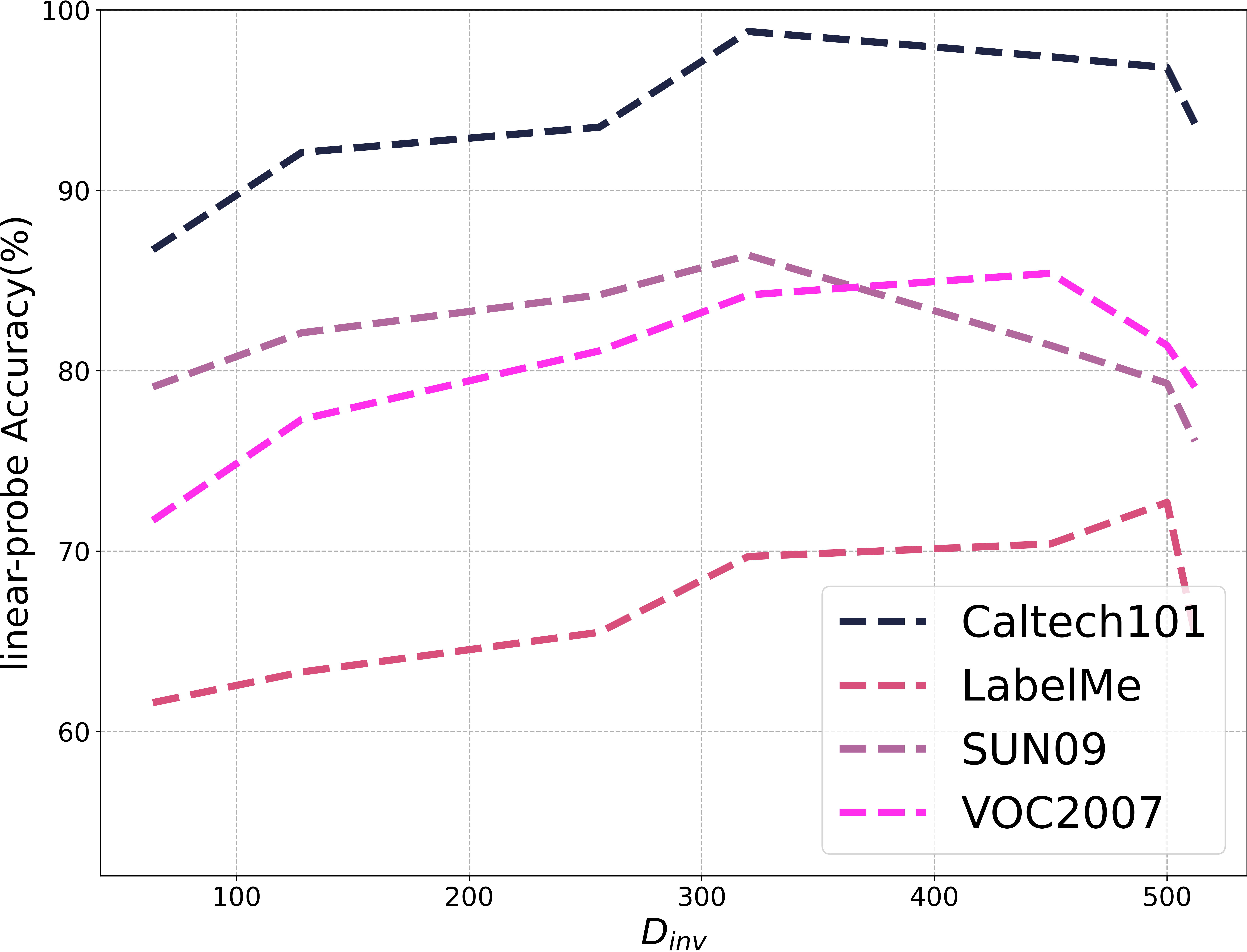
From Figure 8 we can see that as the increases, the accuracy first increases, and stabilizes, and slowly decreases, and finally drops. Therefore, the optimum dimension of should be around to for all domains in VLCS.
Appendix J Ablation study on zero-shot prediction with domain prompt
In experiments from Section 5, we use the standard text prompt template when performing zero-shot prediction, i.e. ”A photo of [cls]” where [cls] is the name of the corresponding class.
To explore the influence of text prompts on zero-shot prediction, we conducted experiments using the PACS, VLCS, and Office-Home datasets. In these experiments, we employed text prompts that incorporate domain information. For datasets where the domain names hold particular significance, such as PACS and Office-Home, we utilized the prompt ’A [domain] of [cls]’. In contrast, for the VLCS dataset, where the domain names do not have specific meanings, we adopted the prompt ’A photo of [cls] in [domain]’. Here, [domain] represents the name of the test domain. The results are illustrated in Table 10, Table 11 and Table 12.
It is important that the objective of domain generalization is to evaluate the performance of a model on unseen domains. Therefore, incorporating domain information, such as (a sketch of [cls]) would not align with the requirements of the domain generalization task. And we only conduct this experiment for exploration.
| Algorithm | Photo | Art | Cartoon | Sketch | Avg |
|---|---|---|---|---|---|
| CLIP | 100.0 | 97.4 | 99.2 | 88.1 | 96.1 |
| CLIP + Domain Prompt | 100.0 | 97.4 | 99.0 | 90.2 | 96.6 |
| CLIP-ICM | 98.7 | 99.1 | 99.9 | 91.7 | 97.3 |
| Algorithm | Caltech101 | LabelMe | SUN09 | VOC2007 | Avg |
|---|---|---|---|---|---|
| CLIP | 99.9 | 70.1 | 73.5 | 86.1 | 82.4 |
| CLIP + Domain Prompt | 99.2 | 69.7 | 65.1 | 80.3 | 78.5 |
| CLIP-ICM | 100.0 | 74.7 | 74.5 | 87.1 | 84.1 |
| Algorithm | Art | Clipart | Product | Real | Avg |
|---|---|---|---|---|---|
| CLIP | 83.3 | 65.3 | 89.0 | 89.3 | 81.7 |
| CLIP + Domain Prompt | 82.4 | 67.0 | 87.8 | 88.7 | 81.4 |
| CLIP-ICM | 83.7 | 67.4 | 90.8 | 90.1 | 82.6 |
From the results in Table 10, we find that only in some domains, incorporating domain information in the prompt template can improve the zero-shot performance, such as Sketch in PACS, and Clipart in Office-Home. However, in most domains, where the domain name doesn’t provide any information, or can’t describe the domain properly, the performance is lower than the original template.
Another important observation is that CLIP-ICM consistently improves the performance of CLIP in most domains, without any domain-related information or other kinds of template design.