3D Unsupervised Learning by Distilling 2D Open-Vocabulary Segmentation Models for Autonomous Driving
Abstract
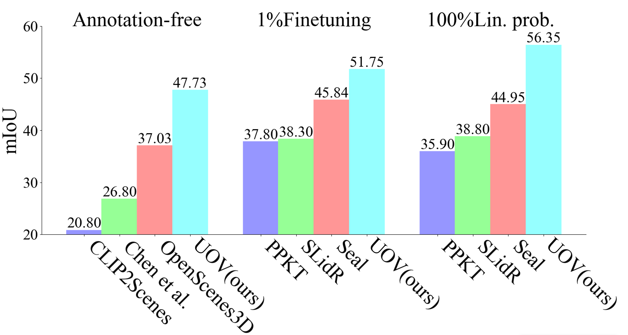
Point cloud data labeling is considered a time-consuming and expensive task in autonomous driving, whereas unsupervised learning can avoid it by learning point cloud representations from unannotated data. In this paper, we propose UOV, a novel 3D Unsupervised framework assisted by 2D Open-Vocabulary segmentation models. It consists of two stages: In the first stage, we innovatively integrate high-quality textual and image features of 2D open-vocabulary models and propose the Tri-Modal contrastive Pre-training (TMP). In the second stage, spatial mapping between point clouds and images is utilized to generate pseudo-labels, enabling cross-modal knowledge distillation. Besides, we introduce the Approximate Flat Interaction (AFI) to address the noise during alignment and label confusion. To validate the superiority of UOV, extensive experiments are conducted on multiple related datasets. We achieved a record-breaking 47.73% mIoU on the annotation-free point cloud segmentation task in nuScenes, surpassing the previous best model by 10.70% mIoU. Meanwhile, the performance of fine-tuning with 1% data on nuScenes and SemanticKITTI reached a remarkable 51.75% mIoU and 48.14% mIoU, outperforming all previous pre-trained models. Our code is available at: https://github.com/sbysbysbys/UOV.
1 Introduction
As neural-network-based 3D scene perception methods, e.g., object detection [1, 2, 3, 4], point cloud segmentation [5, 6, 7], etc., become increasingly complex in their network architectures with a growing number of parameters, methods relying solely on enhancing model structures are reaching a point of saturation. Meanwhile, approaches to enhancing model performance through data-driven methods heavily rely on time-consuming and expensive manual annotations. Due to constraints such as insufficient class annotations, applying traditional point cloud perception methods to large-scale unlabeled data meets significant challenges.
Unsupervised learning is a powerful machine learning paradigm that enables representation learning from data without the need for manually annotated supervision signals. Multi-modal unsupervised algorithms for 3D scene perception tasks integrate the internal structure of point clouds with image or text knowledge to generate objectives. They bypass the costly manual annotations, bridging the gap between traditional 3D perceptual models and unannotated data.
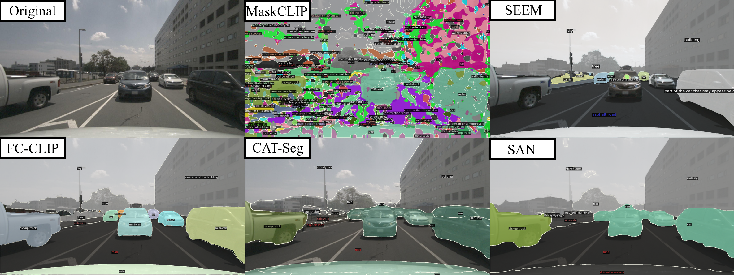
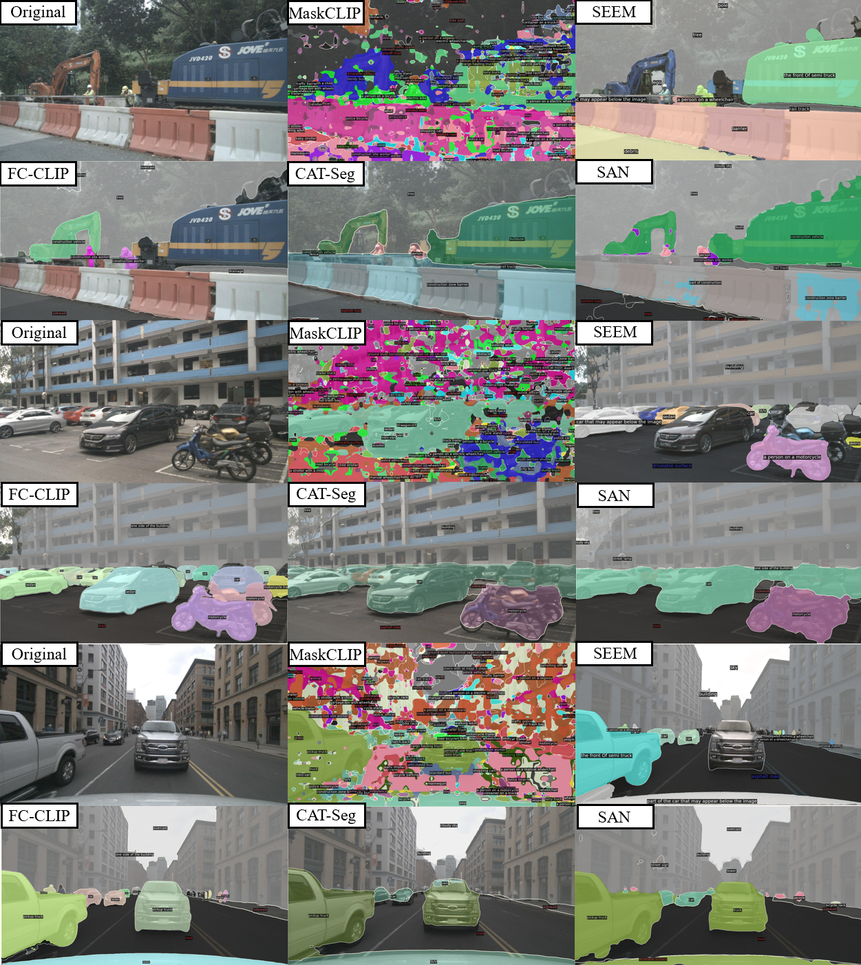
Existing 3D unsupervised methods for annotation-free training [9, 10, 11, 12] aim to transfer knowledge from visual foundation models, e.g., Contrastive Vision-Language Pre-training (CLIP) [13] or Segment Anything (SAM) [14], to point cloud representations. However, 3D unsupervised models based on CLIP [13] suffer from intolerable noise, while SAM [14] fails to correspond texts and images. Therefore, we seek high-quality image segmentation models with textual correspondences to serve as teacher models for 3D unsupervised learning. Recently, CLIP-based 2D open-vocabulary segmentation models [15, 16, 17, 18] have demonstrated excellent performances. They employ contrastive learning to extract textual and image features from a shared embedding space and are capable of segmenting and identifying objects from a set of open classes in various environments. These models provide us with image segmentation and labels corresponding to the segmented regions, as well as easy-to-extract text and image representations. Meanwhile, they significantly outperform other Visual Language Models (VLMs) [13, 19, 20, 21] in open-vocabulary segmentation tasks, as shown in Fig. 3, 6.
In this paper, we propose UOV, a 3D Unsupervised framework by distilling 2D Open-Vocabulary segmentation models. It aims to address the difficulties of point cloud perception using unannotated data through 3D unsupervised learning. Previous work [12, 9] utilizes contrastive learning between point clouds and texts for distilling knowledge, which improves the model’s scene understanding ability but the performance cannot be guaranteed. Hence, one can conclude that using only contrastive learning as the method for annotation-free training is insufficient. Based on this premise, UOV adopts a novel two-stage unsupervised strategy. The first stage uses Tri-Modal contrastive Pre-training (TMP) to warm up the network parameters, where we innovatively incorporate the text modality to enhance the semantic perception of point cloud representations. The training objectives in contrastive loss are all derived from 2D open-vocabulary segmentation models and synchronous generated with segmentations and labels. The second stage is pseudo-label guided annotation-free training, which maps the image segmentation from the 2D open-vocabulary segmentation model to point cloud pseudo-labels, completing the knowledge distillation from 2D to 3D. Meanwhile, it refines semantic comprehension by using a class dictionary, which establishes mappings from open vocabularies to semantic classes. Furthermore, to address the perceptual limitations of images in 3D scenes, such as noise during alignment and label confusion, we introduce Approximate Flat Interaction (AFI), which corrects the error through point cloud spatial interaction over a wide perceptual domain.
In the experiment, We selected four CLIP-based open-vocabulary segmentation models, ie., MaskCLIP [15], FC-CLIP [16], SAN [17], CAT-Seg [18], as teacher models. To validate the performance of our method in unsupervised point cloud segmentation tasks, extensive experiments on multiple autonomous driving datasets were conducted. Firstly, UOV achieved a remarkable improvement of 10.70% mIoU, reaching a Top-1 accuracy of 47.74% mIoU in benchmark testing of annotation-free segmentation performance on nuScenes [8]. Furthermore, to compare the advantages of our approach with previous pre-training methods, we conducted 1% data fine-tuning and 100% data linear-probing experiments on nuScenes, yielding mIoU scores of 51.75% and 56.35%. In comparison to the current best pretraining method, our approach achieved improvements of 5.91% and 11.95% mIoU, respectively. When fine-tuning with 1% data on SemanticKITTI, UOV achieved a 48.14% mIoU, surpassing the previous best method by 1.51% mIoU. UOV demonstrated state-of-the-art performance across various experiments, validating its effectiveness.
Overall, the key contributions of our work are summarized as follows:
1. To the best of our knowledge, our approach not only represents the first attempt to comprehensively utilize state-of-the-art 2D open-vocabulary segmentation models for training 3D unsupervised networks but also the first to synchronously generate knowledge before pre-training and incorporate text featues into pre-training.
2. We propose a two-stage unsupervised framework, UOV, which leverages 2D open-vocabulary segmentation models to assist in unsupervised training without annotation. Additionally, a detachable spatial interaction method, AFI, is introduced to enhance the spatial understanding of the model.
2 Related Work
2.1 CLIP-based 2D Open-Vocabulary Segmentation
2D open-vocabulary segmentation models aim to segment all categories in the real world. Traditional open-vocabulary image segmentation models [22, 23, 24] attempt to learn image embeddings aligned with text embeddings. Inspired by Visual Language Models (VLMs), e.g., CLIP [13] and ALIGN [25], which have demonstrated remarkable performance in 2D tasks, recent studies have attempted to transfer CLIP’s outstanding zero-shot segmentation capability to open-vocabulary tasks [17, 18, 15, 16, 26, 27, 28, 29, 30]. In notable works, LSeg [26] learns pixel-level visual embeddings from CLIP, marking the first exploration of CLIP’s role in language-driven segmentation tasks. More recently, MaskCLIP [15] obtains pixel-level embeddings by modifying the CLIP image encoder. SAN [17] augments CLIP with lightweight side networks to predict mask proposals and categories. CAT-Seg [18] proposes a cost-aggregation-based method to optimize the image-text similarity map. Additionally, FC-CLIP [16] integrates all components into a single-stage framework using a shared frozen convolutional CLIP backbone. These works utilize CLIP as the central component of their network, granting them robust segmentation and recognition capabilities, as well as an image-text-aligned structure. Consequently, they can provide us with high-quality knowledge.
2.2 3D Unsupervised Learning in Large-scale Point Clouds
Unsupervised learning can be utilized for learning point cloud representations. Mainstream 3D unsupervised pre-training methods are mainly reconstruction-based [31, 32, 33, 34], or contrast-based [35, 36, 37, 38, 39, 40, 41]. However, many of these methods are constrained by the quantity of point clouds, limiting their applicability to single-object or indoor scene learning. Prior attempts, such as PointContrast [36], DepthContrast [37], SegContrast [42], and PPKT [38], have built contrastive objectives on large-scale point clouds. Additionally, SLidR [39] adopts a novel approach by leveraging a superpixel-superpoint correspondence for 3D-to-2D spatial alignment, showing promising performance on autonomous driving datasets. Built upon SLidR, SEAL [41] employs VLMs to aid in superpixel generation.
Recently, inspired by the achievements of CLIP [13], numerous works have focused on reproducing the excellent performance demonstrated by CLIP in 3D, not limited to pre-training. In 3D scene understanding, CLIP2Scene [9], similar to OpenScene [12], embeds the knowledge of CLIP feature space into representations of 3D point cloud, enabling annotation-free point cloud segmentation. PLA [43] and RegionPLC [44] accomplish scene understanding through point-language alignment or contrastive learning framework. CLIP2 [10] demonstrates perfect zero-shot instance segmentation performance through language-3D alignment at the semantic level and image-3D alignment at the instance level. Unlike the others, Chen et al. [11] utilizes CLIP to generate pseudo-labels and uses SAM [14] to assist in denoising.
In general, most of these methods rely on either feature alignment or pseudo-labeling. However, using only contrastive learning may incorrectly pull apart positive samples of the same class when employing point-level correspondence methods, e.g., pixel-point, pixel to FPS and -NN. It is also susceptible to differences in data volume for each class and asymmetric point cloud densities. Meanwhile, the use of pseudo-labeling is greatly limited by the accuracy of the teacher’s model. To address these issues, our work employs state-of-the-art 2D open-vocabulary segmentation models as teacher models. We not only distill knowledge onto point cloud using pseudo-labels, but also incorporate multi-modal contrastive learning into our framework.
3 Method
3.1 Extracting Knowledge from CLIP-based 2D Open-Vocabulary Segmentation Models
In perceptual approaches to unknown classes in 2D, unlike zero-shot learning, open-vocabulary learning uses language data as supervision. In terms of network structure, MaskCLIP [15] changes the image encoder of CLIP to propose pixel-level representations instead of image-level. SAN [17] proposes a side adapter network attached to a frozen CLIP encoder; CAT-Seg [18] employs a cost-aggregation-based method to improve CLIP; FC-CLIP [16] adds a decoder, mask generator, in-vocabulary classifier, and out-vocabulary classifier after freezing the CLIP backbone. In most cases, the mask generator operates independently of the class generator. Pixel-level features generated by the modified CLIP-based network are max-pooled for each mask, and the objective loss is computed with the text features.
We can notice that, regardless of whether the CLIP backbone is frozen, whether the CLIP network’s architecture is modified, or whether additional network structures are appended to the side or rear of the CLIP network, the essence of these CLIP-based models lies in aligning image features with text features through contrastive learning.
The aforementioned methods hold a similar view with contrastive learning for point cloud pre-training. The difference is that the latter uses image-point cloud contrastive learning [38, 39] (some of the work uses data augmentation for single-modal contrastive learning). Most of them use SLIC [45], SAM [14], and SEEM [19] to guide mask segmentation and choose ResNet [46] as the image encoder, which means that mask segmentation and mask feature generation are two completely independent modules. This not only increases the training time but also makes noise easily stack up across different models. At the same time, the lack of language guidance during segmentation will lead to a more random mask granularity. Fortunately, 2D open-vocabulary segmentation models perfectly address this issue, as we can not only extract labels and image embeddings from them but also obtain segmentation with appropriate granularity.
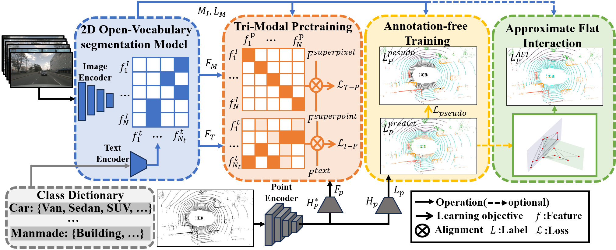
To summarize, we extract four interrelated, synchronously generated knowledge from CLIP-based open-vocabulary segmentation models: 1) images’ segmentations as masks from image set ; 2) corresponding labels for ; 3) image features corresponding to , denoted as ; and 4) text features . Each of the above knowledge will play an important role in Sec. 3.2,3.3,3.4, as shown in Fig. 2.
3.2 Baseline of UOV
Given a point cloud , where represents the 3D coordinates of a point, denotes the point’s features. are the labels of and represents the images captured by a synchronized camera at the same moment. In contrast to supervised methods, our task does not utilize labels during training. We choose to employ a simple way of generating pseudo-labels for point clouds with the assistance of image segmentation: With masks obtained from image set as described in Sec. 3.1, we use the labels corresponding to as the pseudo-label for pixels in every mask . By leveraging known sensor calibration parameters, we establish a mapping to bridge the gap between domains of point clouds and images. Pseudo-labels for point clouds are generated through and mapping . For a 3D backbone with the learnable parameter , we train with pseudo-labels . Given the sparsity of point clouds, it is obvious that is not surjective. It is important to note that is also not injective, as the projection area of LiDAR is not entirely covered by cameras, resulting in obvious pseudo-label-blank areas in point cloud . After knowledge distillation, these untrained regions exhibit label confusion, which will be discussed in Sec. 3.4.
To align open vocabularies with the stuff-classes of autonomous driving datasets, we employ a class dictionary , where represents the number of stuff-classes. Texts belonging to the same class are uniformly mapped to the pseudo-label corresponding to , which implies that points corresponding to and are positive samples for each other.
3.3 Tri-Modal Contrastive Pre-training (TMP)
In CLIP-based 2D open-vocabulary segmentation models, masks and image features mostly share encoders. They are generated synchronously and guided by the same text. On the contrary, to the best of our knowledge, all existing 3D pre-training methods [38, 39, 41] using contrastive learning between image and point cloud generate masks and mask features asynchronously, which causes noise aggregation between different backbones. To break this situation, we introduce Tri-Modal contrastive Pre-training (TMP). TMP innovatively integrates text features into pre-training and removes the 2D backbone through pre-generation of the features, demonstrating excellent performance in both annotation-free training and fine-tuning. The schematic illustration of TMP can refer to Fig. 2.
3.3.1 Superpixel-Superpoint Generation
The usage of superpixels and superpoints for segmentation in SLidR [39] is inspiring, which overturns previous works in 2D-3D contrastive learning methods at the point level. The superpoint-superpixel approach partly alleviates the issue of "self-conflict", which means different point clouds of the same semantics form negative samples in contrastive learning. However, as analyzed in Sec. 3.1, the "self-conflict" problem caused by the mask granularity randomness of VLMs [45, 14] has not been properly addressed. This issue arises due to the lack of textual assistance, e.g., windows and doors of a car should not be treated as negative examples at the granularity of the entire car. On the contrary, 2D open-vocabulary segmentation models [16, 17, 18] perfectly fit the granularity by incorporating textual information defined in class dictionary . Also, as shown in Fig. 3, the accuracy of the superpixels is greatly influenced by the models. Based on these observations, it is reasonable to generate superpixels using CLIP-based 2D open-vocabulary segmentation models.
Given the point cloud and images defined in Sec. 3.2, we have generated masks and use to map the labels of masks to . We regard the set of pixels with corresponding points in the same mask as a superpixel , while the corresponding region of the point cloud as a superpoint , and establish a bijection and ensuring . Assuming the point cloud backbone comes with an output head , we replace with a trainable projection head , projecting the point cloud feature of into a -dimensional space such that , here and refer to mask features and text features provided by the 2D open-vocabulary semantic segmentation models mentioned in Sec. 3.1. Firstly, we apply average pooling and normalization to each group of pixel features guided by superpoints to extract the superpoint embeddings . Then, we normalize as the superpixel embeddings and consider the masks-corresponding text features as . Finally, we employ a tri-modal contrastive loss to align , .
3.3.2 Tri-Modal Contrastive Loss
Superpixel-guided contrastive learning operates at the object level or semantic level, rather than at the pixel or scene level. The contrastive loss between and is formulated as:
| (1) |
where is the feature of superpixel and is the feature of superpoint. denotes the cosine similarity and denotes the temperature coefficient. is the mini-batch size.
Unlike the superpixel-superpoint contrastive loss, the text-superpoint contrastive loss does not exhibit "self-conflict" on classes of a dataset. However, in TMP, to ensure the uniformity of knowledge, we retained the class dictionary as discussed in Sec. 3.2. In UOV-baseline or other downstream tasks, texts of the same class should be considered as positive samples for each other, so treating the point cloud regions corresponding to as negative examples will inadvertently cause "self-conflict". Therefore, for text , we utilize the text feature’s cosine similarity weighted for other texts in the same class as "semi-positive" samples to compute :
| (2) |
| (3) |
where is the text feature corresponding to the mask.
Tri-modal contrastive loss is calculated as:
| (4) |
, are weights for and .
TMP has the following advantages compared to previous pre-training methods: 1) TMP eliminates the need for image encodings during pre-training. It does not require an image backbone, which reduces the training time. 2) Addition of textual modality. Text-superpoint contrastive learning achieves semantic-level alignment, directly endowing the point cloud backbone with semantic features. 3) Synchronous generation of superpixels and . This not only controls segmentation granularity but also prevents the aggregation of noise between different backbones.
3.4 Approximate Flat Interaction
Through Sec. 3.2,3.3, we noticed three technical difficulties for annotation-free semantic segmentation that need to be solved: 1) Unprojected point cloud regions caused by differing or occluded fields of view (FoV) among devices. This directly results in the region of the point cloud outside the image FoV remains untrained for long periods, thus the untrained area suffers from serious label confusion. 2) Label noise. This arises from matching errors between cameras and LiDAR, as well as noise inherent in 2D open-vocabulary segmentation models. 3) Category misperception by single-modal model. Point cloud information struggles to distinguish certain categories across different conditions, whereas information-rich images can address this issue perfectly.
Inspired by Point-NN [47], we propose a non-parametric network for Approximate Flat Interaction (AFI). AFI essentially expects points to interact only among points lying on approximate planes, thereby preserving labels of relatively small objects, e.g., pedestrians, and vehicles, within a broad perceptual domain. The process of AFI is formulated as:
| (5) |
represents the predictions in Sec. 3.2, and indicates the minimum similarity between the directions when their directional features interact. , on the other hand, denotes the point cloud labels predicted by the function . Meanwhile, we can choose to assist optimization through the pseudo-labels generated by 2D open-vocabulary segmentation models. A more detailed description of is stated in Appendix A.
During downsampling, AFI passes the directional features of the sampled center point through layer-wise interactions with neighboring points, and binds the correlation between two points based on 1) whether the two points are relevant in the same direction and 2) the tightness of the relevance between correlated directions. Through four rounds of downsampling, point-to-point interactions construct a network that, apart from points at the junctions, AFI ensures the surfaces formed by points on the same network approximate planes, thus tightly controlling feature interactions among points.
The advantages of AFI are evident. 1) Wide-sensing domain: The perception domain for the point clouds with AFI is wide and possesses strong spatial perception capabilities. 2) Detachability: Not only the entire AFI is detachable, but also the auxiliary module for 2D images within AFI is detachable.The effectiveness of AFI can be referenced in Fig. 5
| Method |
|
|
|
mIoU | ||||||
|---|---|---|---|---|---|---|---|---|---|---|
| CLIP2Scene [9][CVPR’23] | 0% | SPVCNN [48] | 20.80 | |||||||
| Chen et al. [11][NeurIPS’23] | 0% | MinkowskiNet | 26.80 | |||||||
| OpenScene3D [12][CVPR’23] | 0% | MinkowskiNet | 37.03 | |||||||
| UOV(ours)+Mask-clip [15] | 0% | MinkowskiNet | 30.35 | |||||||
| UOV(ours)+FC-CLIP [16] | 0% | MinkowskiNet | 43.28 | |||||||
| UOV(ours)+CAT-Seg [18] | 0% | MinkowskiNet | 42.83 | |||||||
| UOV(ours)+SAN [17] | 0% | MinkowskiNet | 47.73 | |||||||
| OpenScene [12][CVPR’23] | 0% | ✓ | MinkowskiNet | 38.37 | ||||||
| UOV(ours)+FC-CLIP [16] | 0% | ✓ | MinkowskiNet | 43.64 | ||||||
| UOV(ours)+CAT-Seg [18] | 0% | ✓ | MinkowskiNet | 43.64 | ||||||
| UOV(ours)+SAN [17] | 0% | ✓ | MinkowskiNet | 47.89 | ||||||
| - | 100% | MinkowskiNet [7] | 74.66 |
4 Experiments
4.0.1 Datasets
To validate the performance of our model, multiple experiments on two large-scale autonomous driving datasets, nuScenes [8] and SemanticKITTI [49, 50] were conducted, as detailed in Sec. 4.1,4.2. In nuScenes, there are 700 scenes for training, while the validation and test set each consists of 150 scenes, comprising a total of 16 semantic segmentation classes. During pre-training, only the train set was utilized, while we validated using specific scenes separated from the train set. SemanticKITTI has 19 classes, with its 22 sequences partitioned into specific train, validation, and test sets.
4.0.2 Implementation Details
We followed the training paradigm of SLidR [39], employed MinkowskiNet18 [7] as the 3D backbone, and used a linear combination of the cross-entropy and the Lovász loss [51] as training objective in annotation-free and downstream tasks. For 2D open-vocabulary segmentation models, we employed FC-CLIP [16], SAN [17], CAT-Seg [18] for both TMP and annotation-free training, while using MaskCLIP [15] as a control group. The generation of mask features and text features were synchronized with the masks and mask labels. FC-CLIP [16] employed panoptic segmentation, distinguishing different instances on thing-classes. MaskCLIP [15], SAN [17], and CAT-Seg [18] utilized semantic segmentation, not distinguishing instances with the same semantics in both TMP and annotation-free training. Their mask features are selected as the average pool of pixel features in semantically identical regions. In Tri-Modal contrastive Pre-training (TMP) of Sec. 3.3, our network was pre-trained for 40 epochs on 4 V100 GPUs with a batch size of 4, which takes about 80 hours. For annotation-free training in Sec. 3.2 and other downstream tasks, the network was trained for 30 epochs on a single V100 GPU with a batch size of 16, which takes about 18 hours. The temperature coefficient in Eq. 1,2 was set to 0.07, and the optimal results achieved for Eq. 4 when . In Eq. 5 from Sec. 3.4, the minimum similarity between the directions when their directional features interact, was set to 0.995, implying that the maximum angular disparity of two interact point features is about 5.7°. In the network structure of AFI, downsampling was performed four times, with the downsampling rate being for the last three times. Additional details about AFI are provided in Appendix A.
| 3D Initialization | nuScenes | KITTI | |
|---|---|---|---|
| 100%LP | 1%Fine-tuning | 1%Fine-tuning | |
| Random | 8.10 | 30.30 | 39.50 |
| PointConstrast(ECCV’20) [36] | 21.90 | 32.50 | 41.10 |
| DepthConstrast(ICCV’21) [37] | 22.10 | 31.70 | 41.50 |
| PPKT(arXiv’21) [38] | 35.90 | 37.80 | 44.00 |
| SLidR(CVPR’22) [39] | 38.80 | 38.30 | 44.60 |
| ST-SLidR(CVPR’23) [40] | 40.48 | 40.75 | 44.72 |
| Seal(NeurIPS’23) [41] | 44.95 | 45.84 | 46.63 |
| UOV-TMP(ours)+FC-CLIP | 44.24 | 45.73 | 47.02 |
| UOV-TMP(ours)+CAT-Seg | 43.95 | 46.61 | 48.14 |
| UOV-TMP(ours)+SAN | 46.29 | 47.60 | 47.72 |
| UOV(ours)+FC-CLIP | 52.92 | 50.58 | 45.86 |
| UOV(ours)+CAT-Seg | 51.02 | 49.14 | 47.59 |
| UOV(ours)+SAN | 56.35 | 51.75 | 46.60 |
4.1 Comparison Results
4.1.1 Annotation-free Semantic Segmentation
In Tab. 1, we compare UOV with the most closely related works on 3D semantic segmentation using the unannotated data of nuScenes: CLIP2Scene [9] designs a semantic-driven cross-modal contrastive learning framework. Chen et al. [11] utilizes CLIP and SAM for denoising. OpenScene [12] extracts 3D dense features from an open-vocabulary embedding space using multi-view fusion and 3D convolution, we re-implemented its code using MinkowskiNet18. The optimal result of UOV’s single-modal annotation-free segmentation reaches 47.73% mIoU, surpassing the previous best method by 10.70% mIoU, and the gap between the fully supervised same backbone is only -26.93% mIoU. Under image assistance, it achieves 47.89% mIoU.
Compared to the multi-task capability of VLMs, state-of-the-art 2D open-vocabulary segmentation models demonstrate greater capability in specialized domains, as shown in the Fig. 3. Selecting professional teacher models enhances the performance of student models effectively.
4.1.2 Comparisons among 3D Pre-training Methods
We compared the performance of UOV-TMP (only employing TMP) and UOV (employing both steps) against other state-of-the-art methods on multiple downstream tasks in nuScenes and SemanticKITTI, as shown in Tab. 2. All methods utilized MinkowskiNet [7] as the 3D backbone. Most of the compared state-of-the-art methods utilize point cloud-image contrastive learning. SLidR [39] and ST-SLidR [40] employ superpoint-superpixel correspondence granularity, while SEAL [41] employs VLMs to assist in generating superpixels. Our approach achieved optimal results with 1% data fine-tuning on nuScenes and SemanticKITTI, reaching 51.75% mIoU and 48.14% mIoU, respectively, demonstrating a respective improvement of +21.45% mIoU and +8.64% mIoU compared to random initialization. Compared to the previously best results from SEAL, UOV exhibited enhancements of +5.91% mIoU and +1.51% mIoU, respectively. Furthermore, remarkably, the results of the fully supervised linear probing on nuScenes reached 56.35% mIoU, displaying an improvement of +11.40% mIoU compared to SEAL.
4.2 Ablation Study
We conducted a series of ablation experiments on the NuScenes dataset. The ablation targets included different teacher models, TMP, AFI, etc. The results obtained validate the effectiveness of our designs, especially TMP and AFI. Please refer to Appendix B for details of the ablation experiments.
5 Conclusion
We propose UOV, a versatile two-stage unsupervised framework that serves for both 3D pre-training and annotation-free semantic segmentation, achieving state-of-the-art performance across multiple experiments. The key to UOV is to leverage the high-quality knowledge of 2D open-vocabulary segmentation models. Moreover, We propose Tri-Modal contrastive Pre-training (TMP) and Approximate Flat Interaction (AFI) for the first time.
We hope that our work will contribute to more in-depth research on 2D-3D transfer learning. Additionally, to the best of our knowledge, there is currently a lack of work on annotation-free training in other 3D perception tasks such as object detection, trajectory tracking, occupancy grid prediction. We expect the emergence of other annotation-free 3D perception approaches.
References
- [1] Shaoshuai Shi, Xiaogang Wang, and Hongsheng Li. Pointrcnn: 3d object proposal generation and detection from point cloud. In CVPR, 2019.
- [2] Shaoshuai Shi, Chaoxu Guo, Li Jiang, Zhe Wang, Jianping Shi, Xiaogang Wang, and Hongsheng Li. Pv-rcnn: Point-voxel feature set abstraction for 3d object detection. In CVPR, 2020.
- [3] Yin Zhou and Oncel Tuzel. Voxelnet: End-to-end learning for point cloud based 3d object detection. In CVPR, 2018.
- [4] Alex H Lang, Sourabh Vora, Holger Caesar, Lubing Zhou, Jiong Yang, and Oscar Beijbom. Pointpillars: Fast encoders for object detection from point clouds. In CVPR, 2019.
- [5] Charles R Qi, Hao Su, Kaichun Mo, and Leonidas J Guibas. Pointnet: Deep learning on point sets for 3d classification and segmentation. In CVPR, 2017.
- [6] Charles Ruizhongtai Qi, Li Yi, Hao Su, and Leonidas J Guibas. Pointnet++: Deep hierarchical feature learning on point sets in a metric space. In NeurIPS, 2017.
- [7] Christopher Choy, JunYoung Gwak, and Silvio Savarese. 4d spatio-temporal convnets: Minkowski convolutional neural networks. In CVPR, 2019.
- [8] Holger Caesar, Varun Bankiti, Alex H Lang, Sourabh Vora, Venice Erin Liong, Qiang Xu, Anush Krishnan, Yu Pan, Giancarlo Baldan, and Oscar Beijbom. nuscenes: A multimodal dataset for autonomous driving. In CVPR, 2020.
- [9] Runnan Chen, Youquan Liu, Lingdong Kong, Xinge Zhu, Yuexin Ma, Yikang Li, Yuenan Hou, Yu Qiao, and Wenping Wang. Clip2scene: Towards label-efficient 3d scene understanding by clip. In CVPR, 2023.
- [10] Yihan Zeng, Chenhan Jiang, Jiageng Mao, Jianhua Han, Chaoqiang Ye, Qingqiu Huang, Dit-Yan Yeung, Zhen Yang, Xiaodan Liang, and Hang Xu. Clip2: Contrastive language-image-point pretraining from real-world point cloud data. In CVPR, 2023.
- [11] Runnan Chen, Youquan Liu, Lingdong Kong, Nenglun Chen, Xinge Zhu, Yuexin Ma, Tongliang Liu, and Wenping Wang. Towards label-free scene understanding by vision foundation models. arXiv preprint arXiv:2306.03899, 2023.
- [12] Songyou Peng, Kyle Genova, Chiyu Jiang, Andrea Tagliasacchi, Marc Pollefeys, Thomas Funkhouser, et al. Openscene: 3d scene understanding with open vocabularies. In CVPR, 2023.
- [13] Alec Radford, Jong Wook Kim, Chris Hallacy, Aditya Ramesh, Gabriel Goh, Sandhini Agarwal, Girish Sastry, Amanda Askell, Pamela Mishkin, Jack Clark, et al. Learning transferable visual models from natural language supervision. In ICML, 2021.
- [14] Alexander Kirillov, Eric Mintun, Nikhila Ravi, Hanzi Mao, Chloe Rolland, Laura Gustafson, Tete Xiao, Spencer Whitehead, Alexander C Berg, Wan-Yen Lo, et al. Segment anything. 2023.
- [15] Chong Zhou, Chen Change Loy, and Bo Dai. Extract free dense labels from clip. In ECCV, 2022.
- [16] Qihang Yu, Ju He, Xueqing Deng, Xiaohui Shen, and Liang-Chieh Chen. Convolutions die hard: Open-vocabulary segmentation with single frozen convolutional clip. arXiv preprint arXiv:2308.02487, 2023.
- [17] Mengde Xu, Zheng Zhang, Fangyun Wei, Han Hu, and Xiang Bai. Side adapter network for open-vocabulary semantic segmentation. In CVPR, 2023.
- [18] Seokju Cho, Heeseong Shin, Sunghwan Hong, Seungjun An, Seungjun Lee, Anurag Arnab, Paul Hongsuck Seo, and Seungryong Kim. Cat-seg: Cost aggregation for open-vocabulary semantic segmentation. arXiv preprint arXiv:2303.11797, 2023.
- [19] Xueyan Zou, Jianwei Yang, Hao Zhang, Feng Li, Linjie Li, Jianfeng Wang, Lijuan Wang, Jianfeng Gao, and Yong Jae Lee. Segment everything everywhere all at once. In NeurIPS, 2024.
- [20] Xueyan Zou, Zi-Yi Dou, Jianwei Yang, Zhe Gan, Linjie Li, Chunyuan Li, Xiyang Dai, Harkirat Behl, Jianfeng Wang, Lu Yuan, et al. Generalized decoding for pixel, image, and language. In CVPR, 2023.
- [21] Feng Li, Hao Zhang, Peize Sun, Xueyan Zou, Shilong Liu, Jianwei Yang, Chunyuan Li, Lei Zhang, and Jianfeng Gao. Semantic-sam: Segment and recognize anything at any granularity. arXiv preprint arXiv:2307.04767, 2023.
- [22] Hang Zhao, Xavier Puig, Bolei Zhou, Sanja Fidler, and Antonio Torralba. Open vocabulary scene parsing. In ICCV, 2017.
- [23] Yongqin Xian, Subhabrata Choudhury, Yang He, Bernt Schiele, and Zeynep Akata. Semantic projection network for zero-and few-label semantic segmentation. In CVPR, 2019.
- [24] Maxime Bucher, Tuan-Hung Vu, Matthieu Cord, and Patrick Pérez. Zero-shot semantic segmentation. In NeurIPS, 2019.
- [25] Chao Jia, Yinfei Yang, Ye Xia, Yi-Ting Chen, Zarana Parekh, Hieu Pham, Quoc Le, Yun-Hsuan Sung, Zhen Li, and Tom Duerig. Scaling up visual and vision-language representation learning with noisy text supervision. In ICML, 2021.
- [26] Boyi Li, Kilian Q Weinberger, Serge Belongie, Vladlen Koltun, and René Ranftl. Language-driven semantic segmentation, 2022.
- [27] Golnaz Ghiasi, Xiuye Gu, Yin Cui, and Tsung-Yi Lin. Scaling open-vocabulary image segmentation with image-level labels. In ECCV, 2022.
- [28] Jian Ding, Nan Xue, Gui-Song Xia, and Dengxin Dai. Decoupling zero-shot semantic segmentation. In CVPR, 2022.
- [29] Mengde Xu, Zheng Zhang, Fangyun Wei, Yutong Lin, Yue Cao, Han Hu, and Xiang Bai. A simple baseline for open-vocabulary semantic segmentation with pre-trained vision-language model. In ECCV, 2022.
- [30] Feng Liang, Bichen Wu, Xiaoliang Dai, Kunpeng Li, Yinan Zhao, Hang Zhang, Peizhao Zhang, Peter Vajda, and Diana Marculescu. Open-vocabulary semantic segmentation with mask-adapted clip. In CVPR, 2023.
- [31] Alexandre Boulch, Corentin Sautier, Björn Michele, Gilles Puy, and Renaud Marlet. Also: Automotive lidar self-supervision by occupancy estimation. In CVPR, 2023.
- [32] Zhiwei Lin and Yongtao Wang. Bev-mae: Bird’s eye view masked autoencoders for outdoor point cloud pre-training. arXiv preprint arXiv:2212.05758, 2022.
- [33] Georg Hess, Johan Jaxing, Elias Svensson, David Hagerman, Christoffer Petersson, and Lennart Svensson. Masked autoencoder for self-supervised pre-training on lidar point clouds. In WACV, 2023.
- [34] Chen Min, Liang Xiao, Dawei Zhao, Yiming Nie, and Bin Dai. Occupancy-mae: Self-supervised pre-training large-scale lidar point clouds with masked occupancy autoencoders. TIV, 2023.
- [35] Zhenyu Li, Zehui Chen, Ang Li, Liangji Fang, Qinhong Jiang, Xianming Liu, Junjun Jiang, Bolei Zhou, and Hang Zhao. Simipu: Simple 2d image and 3d point cloud unsupervised pre-training for spatial-aware visual representations. In AAAI, 2022.
- [36] Saining Xie, Jiatao Gu, Demi Guo, Charles R Qi, Leonidas Guibas, and Or Litany. Pointcontrast: Unsupervised pre-training for 3d point cloud understanding. In ECCV, 2020.
- [37] Zaiwei Zhang, Rohit Girdhar, Armand Joulin, and Ishan Misra. Self-supervised pretraining of 3d features on any point-cloud. In ICCV, 2021.
- [38] Yueh-Cheng Liu, Yu-Kai Huang, Hung-Yueh Chiang, Hung-Ting Su, Zhe-Yu Liu, Chin-Tang Chen, Ching-Yu Tseng, and Winston H Hsu. Learning from 2d: Contrastive pixel-to-point knowledge transfer for 3d pretraining. arXiv preprint arXiv:2104.04687, 2021.
- [39] Corentin Sautier, Gilles Puy, Spyros Gidaris, Alexandre Boulch, Andrei Bursuc, and Renaud Marlet. Image-to-lidar self-supervised distillation for autonomous driving data. In CVPR, 2022.
- [40] Anas Mahmoud, Jordan SK Hu, Tianshu Kuai, Ali Harakeh, Liam Paull, and Steven L Waslander. Self-supervised image-to-point distillation via semantically tolerant contrastive loss. In CVPR, 2023.
- [41] Youquan Liu, Lingdong Kong, Jun Cen, Runnan Chen, Wenwei Zhang, Liang Pan, Kai Chen, and Ziwei Liu. Segment any point cloud sequences by distilling vision foundation models. arXiv preprint arXiv:2306.09347, 2023.
- [42] Lucas Nunes, Rodrigo Marcuzzi, Xieyuanli Chen, Jens Behley, and Cyrill Stachniss. Segcontrast: 3d point cloud feature representation learning through self-supervised segment discrimination. RAL, 2022.
- [43] Runyu Ding, Jihan Yang, Chuhui Xue, Wenqing Zhang, Song Bai, and Xiaojuan Qi. Pla: Language-driven open-vocabulary 3d scene understanding. In CVPR, 2023.
- [44] Jihan Yang, Runyu Ding, Zhe Wang, and Xiaojuan Qi. Regionplc: Regional point-language contrastive learning for open-world 3d scene understanding. arXiv preprint arXiv:2304.00962, 2023.
- [45] Radhakrishna Achanta, Appu Shaji, Kevin Smith, Aurelien Lucchi, Pascal Fua, and Sabine Süsstrunk. Slic superpixels compared to state-of-the-art superpixel methods. TPAMI, 2012.
- [46] Kaiming He, Xiangyu Zhang, Shaoqing Ren, and Jian Sun. Deep residual learning for image recognition. In CVPR, 2016.
- [47] Renrui Zhang, Liuhui Wang, Yali Wang, Peng Gao, Hongsheng Li, and Jianbo Shi. Parameter is not all you need: Starting from non-parametric networks for 3d point cloud analysis. arXiv preprint arXiv:2303.08134, 2023.
- [48] Haotian Tang, Zhijian Liu, Shengyu Zhao, Yujun Lin, Ji Lin, Hanrui Wang, and Song Han. Searching efficient 3d architectures with sparse point-voxel convolution. In ECCV, 2020.
- [49] Jens Behley, Martin Garbade, Andres Milioto, Jan Quenzel, Sven Behnke, Cyrill Stachniss, and Jurgen Gall. Semantickitti: A dataset for semantic scene understanding of lidar sequences. In ICCV, 2019.
- [50] Andreas Geiger, Philip Lenz, and Raquel Urtasun. Are we ready for autonomous driving? the kitti vision benchmark suite. In CVPR, 2012.
- [51] Maxim Berman, Amal Rannen Triki, and Matthew B. Blaschko. The lovász-softmax loss: A tractable surrogate for the optimization of the intersection-over-union measure in neural networks. In CVPR, 2018.
- [52] Tsung-Yi Lin, Michael Maire, Serge Belongie, James Hays, Pietro Perona, Deva Ramanan, Piotr Dollár, and C Lawrence Zitnick. Microsoft coco: Common objects in context. In ECCV, 2014.
- [53] Xinlei Chen, Haoqi Fan, Ross Girshick, and Kaiming He. Improved baselines with momentum contrastive learning. arXiv preprint arXiv:2003.04297, 2020.
- [54] Kaiming He, Haoqi Fan, Yuxin Wu, Saining Xie, and Ross Girshick. Momentum contrast for unsupervised visual representation learning. In CVPR, 2020.
Appendix A Approximate Flat Interaction (AFI)
Firstly, we remove the predictions in the label-confused area. Then, we utilize pseudo-labels generated in Sec. 3.2 to randomly cover model-predicted labels (note that the coverage step is optional). The probability for random covering point is defined as follows:
| (6) |
Here, variable represents the horizontal distance of point , donates the ratio of the occurrence probabilities of pseudo labels and predicts labels when , and represents the horizontal distance when . We set and in Eq. 6.
Secondly, we need to fill large unannotated regions and eliminate noise introduced by 2D open-vocabulary segmentation models:
For a set of regional point clouds with corresponding features , assuming the center of is , We try to perform directional clustering of relative coordinates for points excluding . Considering the limited temporal effectiveness of conventional clustering methods, a novel way is explored:
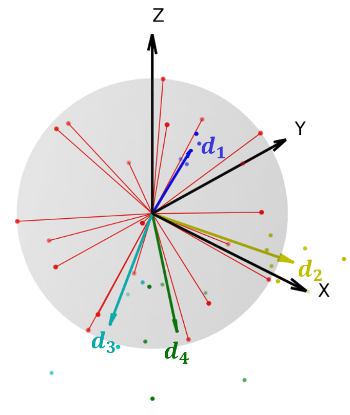
We obtain the spherical Fibonacci lattice of the sphere by the following equation, where for , the normal vector for each point on the grid is denoted as:
| (7) |
where is the golden ratio. Normal vectors is shown in Fig. 4a.
After that, we perform clustering by calculating the cosine similarity between the relative coordinates of to and normal vectors .
| (8) |
After clustering, the mean direction vector , direction feature , and correlation are computed for each normal vector , where :
| (9) |
where denotes the average function, and represents the correlation between each point and the central point . It is worth noting that during the first downsampling, the correlation is the proportion of points belonging to the same direction, ie., . However, in subsequent downsampling steps, the correlation is obtained through the interaction among point cloud and other neighbor point clouds. This implies that we need to transmit the correlations and the mean direction vectors along with the coordinates and features from the previous layer.
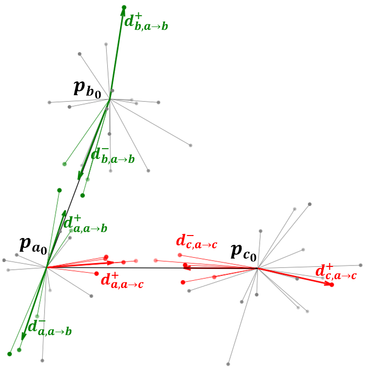
As shown in Fig. 4b, in downsamplings, assuming the mean direction vectors and correlations for two interacting point clouds , are (, ) and (, ), respectively. Assuming the direction from the center of point cloud to the center of point cloud is the positive direction, we calculate the cosine similarity between the vector connecting two central points and the mean direction vectors , :
| (10) |
| (11) |
Afterward we obtain the index sets of approximate-parallel vectors in positive and negative directions:
| (12) |
where represents the minimum arccosine value of two vectors recognized as approximately parallel, which is the same as defined in Eq. 5. represents the distance of , and so forth.
Through the aforementioned sets of approximate-parallel vectors, we can obtain the correlation from point cloud to , which is computed by multiplying two components: the correlation along the approximately parallel direction , and the correlation based on the distance :
| (13) |
| (14) |
| (15) |
During the last three downsamplings, for point cloud , we obtain the correlation of every surrounding point around a central point through Eq. 10,11,12,13,14,15. Among them, and utilized in Eq. 10,11 correspond to the computation results of point and in the previous layer. Afterwards, is converted to a probability distribution using softmax:
| (16) |
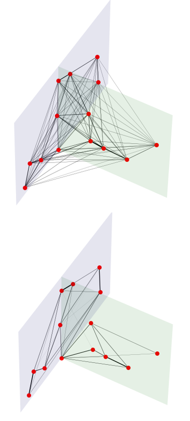
Through Eq. 10,11,12,13,14,15,16, we use the mean direction vectors , correlations and features generated before each downsampling step to assist in generating the new correlation for each point around . Then we use Eq. 9 to obtain from and from . Afterwords acts as weights for the directional features and contributes to the generation of central point features (Eq. 17). Throughout the entire process, we bind the correlation between two points to 1) whether they are relevant in the same direction (corresponding to in Eq. 13), and 2) how close the relevance is between the correlated directions (corresponding to in Eq. 14). Through four rounds of downsampling, point-to-point interactions construct an approximate flat network, thus tightly controlling feature interactions among points (Fig. 4c).
Neural Network Architecture:
Encoder: For point cloud , we use one-hot encoding of the predict labels in Eq. 5 as pseudo-features for point . Within each layer of the encoder, we first employ the farthest point sampling (FPS) followed by -nearest neighbors (-NN) for downsampling. It is necessary to transmit the mean direction vectors and correlations from the previous layer’s output during downsampling. Then, using Eq. 7,8,9,10,11,12,13,14,15,16, we calculate the mean direction vectors , features and correlations for each point . Next, for each central point , we use the following formula to generate the new point feature :
| (17) |
where is the original point feature, and represents original features of points in the neighborhood. The softmax operates on the features.
Decoder: Similar to the operations in the encoder, the upsampling layer of the decoder utilizes the directional correlations generated at each layer of the encoder. After selecting nearest neighbors, the impact of distance on the upsampling weights is discarded:
| (18) |
where represents the original features of points in the neighborhood. denotes the correlation between and neighbor in direction , represents the features of corresponding points in the encoder’s same layer (Eq. 17). The definition of is consistent with Eq. 10,11.
Finally, we obtain the labels at the final layer of the decoder.
Appendix B Ablation Study
|
Baseline | +TMP | +AFI |
|
|
|
||||||||
|---|---|---|---|---|---|---|---|---|---|---|---|---|---|---|
| MaskCLIP(ECCV’22) [15] | 25.49 | - | 30.35 | 27.76 | - | - | ||||||||
| FC-CLIP(NeurIPS’23) [16] | 39.00 | 41.70 | 41.89 | 42.44 | 43.28 | 43.64 | ||||||||
| CAT-Seg(arXiv’23) [18] | 38.45 | 40.92 | 41.79 | 42.50 | 42.83 | 43.64 | ||||||||
| SAN(CVPR’23) [17] | 44.16 | 47.42 | 46.26 | 46.92 | 47.73 | 47.89 |
| 2D Teacher Model | COCO (% mIoU) | Segment task | pseudo-label | pseudo-label | |||
|---|---|---|---|---|---|---|---|
| A-847 | PC-459 | A-150 | PC-59 | coverage rate | Acc | ||
| MaskCLIP(ECCV’22) [15] | 8.2 | 10.0 | 23.7 | 45.9 | Semantic | 55.00 | 50.18 |
| FC-CLIP(NeurIPS’23) [16] | 14.8 | 18.2 | 34.1 | 58.4 | panoptic | 45.95 | 78.96 |
| CAT-Seg(arXiv’23) [18] | 10.8 | 20.4 | 31.5 | 62.0 | Semantic | 55.00 | 77.05 |
| SAN(CVPR’23) [17] | 13.7 | 17.1 | 33.3 | 60.2 | Semantic | 55.00 | 80.38 |
For the ablation study on different setups of UOV (Tab. 3), we utilized MaskCLIP [15] as the control group, and FC-CLIP [16], CAT-Seg [18], and SAN [17] as the experimental groups. Several sets of experiments were conducted while controlling for irrelevant variables. Meanwhile, for a deeper understanding of the impact of certain ablation targets, we conducted separate experiments employing CAT-Seg as the teacher model, as illustrated in the Tab. 5.
Performance Gap in Transferring 2D Open-Vocabulary Segmentation Models to 3D Tasks As shown in Tab. 3, when conducting ablation experiments with different experimental groups, SAN consistently outperforms FC-CLIP and CAT-Seg under any configuration, achieving a 44.16% mIoU in the UOV-baseline, which is 5.16% mIoU and 5.71% mIoU higher than the latter two. We record the accuracy (Acc) of different 2D open-vocabulary segmentation models in generating point cloud pseudo-labels in Tab. 4, while also providing their performance on open-vocabulary segmentation in COCO [52]. We believe that the reasons different teacher models affect student models performance are 1) the ability to comprehend unknown classes, which can affect the accuracy of pseudo-labels, as the number of unknown classes in the class dictionary is far greater than that of known classes; Meanwhile, 2) the degree of alignment between image and text features, with SAN exhibiting the largest disparity, making the fitting of the objective loss Eq. 1,2 more challenging during TMP. It is worth noting that models trained with FC-CLIP and CAT-Seg, even after TMP and AFI, do not outperform the baseline of SAN on annotation-free segmentation. This indicates that A Great Teacher Model is All You Need.
The Role of Class Dictionary The class dictionary serves to bridge the datasets’ stuff-classes with open vocabularies. Directly inputting semantic classes of the dataset as prompts into 2D open-vocabulary segmentation models is inefficient, as open-vocabulary models are better suited to understand prompts with smaller semantic granularity. As observed in Tab. 5, not using a class dictionary resulted in a -22.85% mIoU decrease compared to using one.
| TMP | AFI | annotation-free | 1%fine-tune | ||||||||
|---|---|---|---|---|---|---|---|---|---|---|---|
| ✓ |
|
|
|||||||||
| ✓ | ✓ | 39.62(+1.17) | 43.31(+5.01) | ||||||||
| ✓ | ✓ | ✓ | 40.49(+2.04) | 45.83(+7.53) | |||||||
| ✓ | ✓ | ✓ | 39.84(+1.39) | 43.70(+5.40) | |||||||
| ✓ | ✓ | ✓ | ✓ | 40.92(+2.47) | 46.61(+8.31) | ||||||
| 15.60(-22.85) | - | ||||||||||
| ✓ | ✓ | ✓ | ✓ | 40.92(+2.47) | - | ||||||
| ✓ | ✓ | ✓ | ✓ | ✓ | 42.83(+4.38) | - | |||||
| ✓ | ✓ | ✓ | ✓ | ✓ | ✓ | 43.64(+5.19) | - |
Ablation Targets in TMP In Tab. 5, employing CAT-Seg [18] as the teacher model, we investigate the efficacy of TMP through two ablation experiments: 1) replacing image features with the outputs of self-supervised ResNet50 [46] backbone using MoCov2 [53, 54], and 2) excluding text-point contrastive loss . Results from fine-tuning with 1% data and annotation-free point cloud segmentation experiments demonstrate the superiority of TMP over both 1) and 2). Moreover, we affirm the positive impact of TMP on the task of annotation-free point cloud segmentation. As we can see from Tab. 3, incorporating TMP into baselines of FC-CLIP, CAT-Seg, and SAN improved their respective scores by 2.7% mIoU, 2.47% mIoU, and 3.26% mIoU, compared to pre-training with SLidR [39].
Effect of AFI AFI leverages 3D spatial information to enhance the segmentation of unannotated point clouds. Employing AFI on models of FC-CLIP, CAT-Seg, and SAN reached 41.89%, 41.79%, and 46.26% mIoU, a boost of 2.89%, 3.34%, and 2.1% mIoU over their baseline (Tab. 3). It is noteworthy that the combined usage of TMP and AFI results in a greater improvement compared to using either one alone. However, this improvement is not linearly additive.
The Role of Pseudo-Label Guided Knowledge Distillation in Fine-tuning Tasks It is important to note that if we treat UOV as a pre-training method, it does not utilize the validation set in either stage. The two-stage UOV outperforms the one-stage UOV-TMP for downstream tasks on nuScenes, as shown in Tab. 2. The superiority arises from the second-stage annotation-free training and the downstream tasks employing the same loss function, which is particularly effective during linear probing. However, annotation-free training weakens the model’s generalization ability, resulting in inferior performance when transferred to other datasets, e.g., downstream tasks on SemanticKITTI (pre-trained on nuScenes) compared to using only TMP.
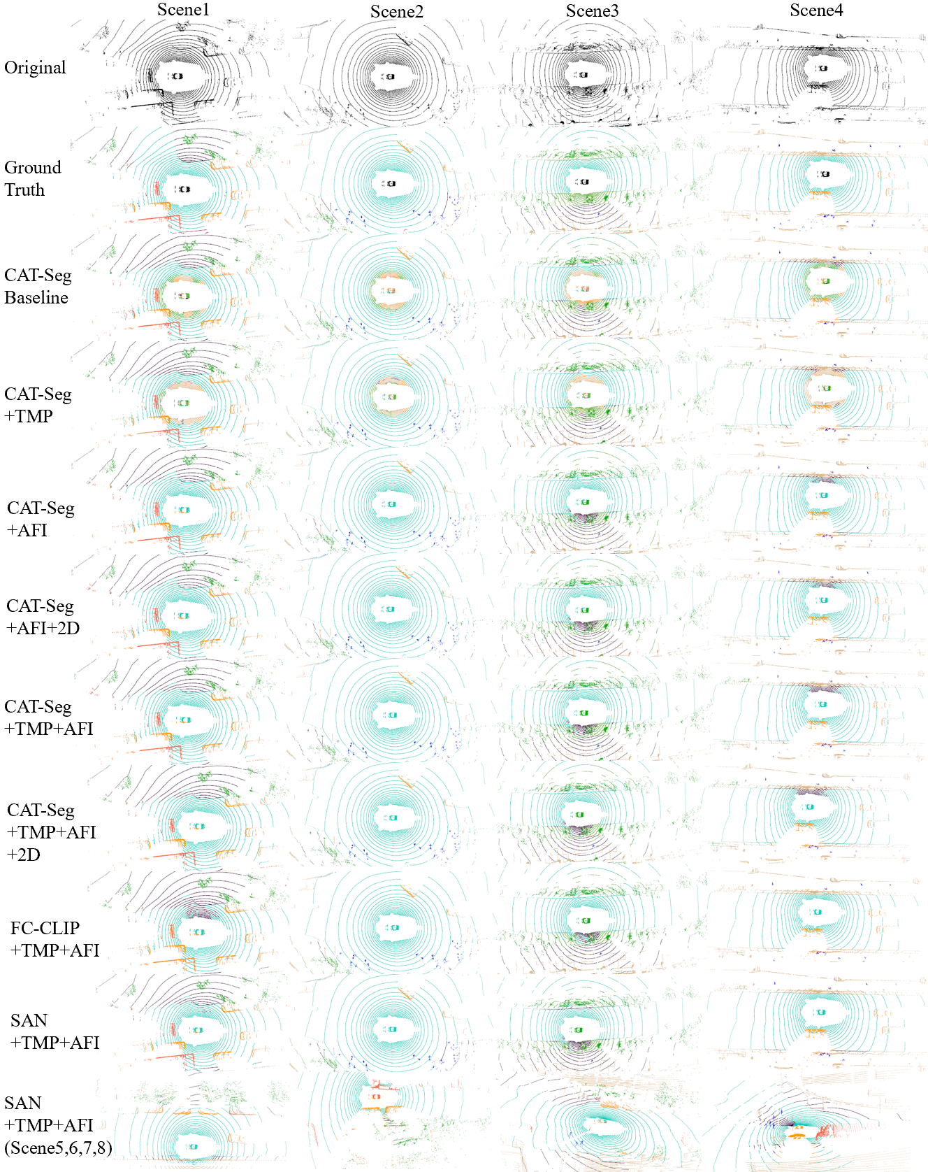
We present additional annotation-free segmentation results in Fig. 5.
Appendix C Liminations
Our framework can utilize image assistance during annotation-free segmentation, which is accomplished through post-processing with pseudo labels generated by 2D open-vocabulary models. However, our image assistance offers limited improvement (an average increase of 0.5% mIoU). Moreover, this work primarily addresses annotation-free learning tasks, wherein pseudo-labels are employed during training, resulting in a relatively weak understanding of point clouds. Besides, due to the specificity of the class dictionary and AFI, it may only be suitable for segmenting outdoor point clouds.
Appendix D Attached Diagrams
NeurIPS Paper Checklist
-
1.
Claims
-
Question: Do the main claims made in the abstract and introduction accurately reflect the paper’s contributions and scope?
-
Answer: [Yes]
-
Justification: We clearly articulated the contributions and innovations of this paper in the abstract and introduction.
-
Guidelines:
-
•
The answer NA means that the abstract and introduction do not include the claims made in the paper.
-
•
The abstract and/or introduction should clearly state the claims made, including the contributions made in the paper and important assumptions and limitations. A No or NA answer to this question will not be perceived well by the reviewers.
-
•
The claims made should match theoretical and experimental results, and reflect how much the results can be expected to generalize to other settings.
-
•
It is fine to include aspirational goals as motivation as long as it is clear that these goals are not attained by the paper.
-
•
-
2.
Limitations
-
Question: Does the paper discuss the limitations of the work performed by the authors?
-
Answer: [Yes]
-
Justification: We discuss the limitations of our work in Appendix C.
-
Guidelines:
-
•
The answer NA means that the paper has no limitation while the answer No means that the paper has limitations, but those are not discussed in the paper.
-
•
The authors are encouraged to create a separate "Limitations" section in their paper.
-
•
The paper should point out any strong assumptions and how robust the results are to violations of these assumptions (e.g., independence assumptions, noiseless settings, model well-specification, asymptotic approximations only holding locally). The authors should reflect on how these assumptions might be violated in practice and what the implications would be.
-
•
The authors should reflect on the scope of the claims made, e.g., if the approach was only tested on a few datasets or with a few runs. In general, empirical results often depend on implicit assumptions, which should be articulated.
-
•
The authors should reflect on the factors that influence the performance of the approach. For example, a facial recognition algorithm may perform poorly when image resolution is low or images are taken in low lighting. Or a speech-to-text system might not be used reliably to provide closed captions for online lectures because it fails to handle technical jargon.
-
•
The authors should discuss the computational efficiency of the proposed algorithms and how they scale with dataset size.
-
•
If applicable, the authors should discuss possible limitations of their approach to address problems of privacy and fairness.
-
•
While the authors might fear that complete honesty about limitations might be used by reviewers as grounds for rejection, a worse outcome might be that reviewers discover limitations that aren’t acknowledged in the paper. The authors should use their best judgment and recognize that individual actions in favor of transparency play an important role in developing norms that preserve the integrity of the community. Reviewers will be specifically instructed to not penalize honesty concerning limitations.
-
•
-
3.
Theory Assumptions and Proofs
-
Question: For each theoretical result, does the paper provide the full set of assumptions and a complete (and correct) proof?
-
Answer: [N/A]
-
Justification: Our paper focus on annotation-free point cloud segmentation and 3D pre-training, it does not include theoretical results.
-
Guidelines:
-
•
The answer NA means that the paper does not include theoretical results.
-
•
All the theorems, formulas, and proofs in the paper should be numbered and cross-referenced.
-
•
All assumptions should be clearly stated or referenced in the statement of any theorems.
-
•
The proofs can either appear in the main paper or the supplemental material, but if they appear in the supplemental material, the authors are encouraged to provide a short proof sketch to provide intuition.
-
•
Inversely, any informal proof provided in the core of the paper should be complemented by formal proofs provided in appendix or supplemental material.
-
•
Theorems and Lemmas that the proof relies upon should be properly referenced.
-
•
-
4.
Experimental Result Reproducibility
-
Question: Does the paper fully disclose all the information needed to reproduce the main experimental results of the paper to the extent that it affects the main claims and/or conclusions of the paper (regardless of whether the code and data are provided or not)?
-
Answer: [Yes]
-
Guidelines:
-
•
The answer NA means that the paper does not include experiments.
-
•
If the paper includes experiments, a No answer to this question will not be perceived well by the reviewers: Making the paper reproducible is important, regardless of whether the code and data are provided or not.
-
•
If the contribution is a dataset and/or model, the authors should describe the steps taken to make their results reproducible or verifiable.
-
•
Depending on the contribution, reproducibility can be accomplished in various ways. For example, if the contribution is a novel architecture, describing the architecture fully might suffice, or if the contribution is a specific model and empirical evaluation, it may be necessary to either make it possible for others to replicate the model with the same dataset, or provide access to the model. In general. releasing code and data is often one good way to accomplish this, but reproducibility can also be provided via detailed instructions for how to replicate the results, access to a hosted model (e.g., in the case of a large language model), releasing of a model checkpoint, or other means that are appropriate to the research performed.
-
•
While NeurIPS does not require releasing code, the conference does require all submissions to provide some reasonable avenue for reproducibility, which may depend on the nature of the contribution. For example
-
(a)
If the contribution is primarily a new algorithm, the paper should make it clear how to reproduce that algorithm.
-
(b)
If the contribution is primarily a new model architecture, the paper should describe the architecture clearly and fully.
-
(c)
If the contribution is a new model (e.g., a large language model), then there should either be a way to access this model for reproducing the results or a way to reproduce the model (e.g., with an open-source dataset or instructions for how to construct the dataset).
-
(d)
We recognize that reproducibility may be tricky in some cases, in which case authors are welcome to describe the particular way they provide for reproducibility. In the case of closed-source models, it may be that access to the model is limited in some way (e.g., to registered users), but it should be possible for other researchers to have some path to reproducing or verifying the results.
-
(a)
-
•
-
5.
Open access to data and code
-
Question: Does the paper provide open access to the data and code, with sufficient instructions to faithfully reproduce the main experimental results, as described in supplemental material?
-
Answer: [Yes]
-
Justification: We offer codes in the supplementary materials, as well as an anonymous repository (https://anonymous.4open.science/r/UOV2024) for easy access.
-
Guidelines:
-
•
The answer NA means that paper does not include experiments requiring code.
-
•
Please see the NeurIPS code and data submission guidelines (https://nips.cc/public/guides/CodeSubmissionPolicy) for more details.
-
•
While we encourage the release of code and data, we understand that this might not be possible, so “No” is an acceptable answer. Papers cannot be rejected simply for not including code, unless this is central to the contribution (e.g., for a new open-source benchmark).
-
•
The instructions should contain the exact command and environment needed to run to reproduce the results. See the NeurIPS code and data submission guidelines (https://nips.cc/public/guides/CodeSubmissionPolicy) for more details.
-
•
The authors should provide instructions on data access and preparation, including how to access the raw data, preprocessed data, intermediate data, and generated data, etc.
-
•
The authors should provide scripts to reproduce all experimental results for the new proposed method and baselines. If only a subset of experiments are reproducible, they should state which ones are omitted from the script and why.
-
•
At submission time, to preserve anonymity, the authors should release anonymized versions (if applicable).
-
•
Providing as much information as possible in supplemental material (appended to the paper) is recommended, but including URLs to data and code is permitted.
-
•
-
6.
Experimental Setting/Details
-
Question: Does the paper specify all the training and test details (e.g., data splits, hyperparameters, how they were chosen, type of optimizer, etc.) necessary to understand the results?
-
Answer: [Yes]
-
Justification: We provide all the training and test details in Sec. 4.0.2, as well as in our code.
-
Guidelines:
-
•
The answer NA means that the paper does not include experiments.
-
•
The experimental setting should be presented in the core of the paper to a level of detail that is necessary to appreciate the results and make sense of them.
-
•
The full details can be provided either with the code, in appendix, or as supplemental material.
-
•
-
7.
Experiment Statistical Significance
-
Question: Does the paper report error bars suitably and correctly defined or other appropriate information about the statistical significance of the experiments?
-
Answer: [No]
-
Justification: Error bars are not reported because it would be too computationally expensive.
-
Guidelines:
-
•
The answer NA means that the paper does not include experiments.
-
•
The authors should answer "Yes" if the results are accompanied by error bars, confidence intervals, or statistical significance tests, at least for the experiments that support the main claims of the paper.
-
•
The factors of variability that the error bars are capturing should be clearly stated (for example, train/test split, initialization, random drawing of some parameter, or overall run with given experimental conditions).
-
•
The method for calculating the error bars should be explained (closed form formula, call to a library function, bootstrap, etc.)
-
•
The assumptions made should be given (e.g., Normally distributed errors).
-
•
It should be clear whether the error bar is the standard deviation or the standard error of the mean.
-
•
It is OK to report 1-sigma error bars, but one should state it. The authors should preferably report a 2-sigma error bar than state that they have a 96% CI, if the hypothesis of Normality of errors is not verified.
-
•
For asymmetric distributions, the authors should be careful not to show in tables or figures symmetric error bars that would yield results that are out of range (e.g. negative error rates).
-
•
If error bars are reported in tables or plots, The authors should explain in the text how they were calculated and reference the corresponding figures or tables in the text.
-
•
-
8.
Experiments Compute Resources
-
Question: For each experiment, does the paper provide sufficient information on the computer resources (type of compute workers, memory, time of execution) needed to reproduce the experiments?
-
Answer: [Yes]
-
Justification: We provide the information about computing resources in Sec. 4.0.2.
-
Guidelines:
-
•
The answer NA means that the paper does not include experiments.
-
•
The paper should indicate the type of compute workers CPU or GPU, internal cluster, or cloud provider, including relevant memory and storage.
-
•
The paper should provide the amount of compute required for each of the individual experimental runs as well as estimate the total compute.
-
•
The paper should disclose whether the full research project required more compute than the experiments reported in the paper (e.g., preliminary or failed experiments that didn’t make it into the paper).
-
•
-
9.
Code Of Ethics
-
Question: Does the research conducted in the paper conform, in every respect, with the NeurIPS Code of Ethics https://neurips.cc/public/EthicsGuidelines?
-
Answer: [Yes]
-
Justification: This research paper complies with the NeurIPS Code of Ethics.
-
Guidelines:
-
•
The answer NA means that the authors have not reviewed the NeurIPS Code of Ethics.
-
•
If the authors answer No, they should explain the special circumstances that require a deviation from the Code of Ethics.
-
•
The authors should make sure to preserve anonymity (e.g., if there is a special consideration due to laws or regulations in their jurisdiction).
-
•
-
10.
Broader Impacts
-
Question: Does the paper discuss both potential positive societal impacts and negative societal impacts of the work performed?
-
Answer: [N/A]
-
Justification: There is no societal impact of the work performed.
-
Guidelines:
-
•
The answer NA means that there is no societal impact of the work performed.
-
•
If the authors answer NA or No, they should explain why their work has no societal impact or why the paper does not address societal impact.
-
•
Examples of negative societal impacts include potential malicious or unintended uses (e.g., disinformation, generating fake profiles, surveillance), fairness considerations (e.g., deployment of technologies that could make decisions that unfairly impact specific groups), privacy considerations, and security considerations.
-
•
The conference expects that many papers will be foundational research and not tied to particular applications, let alone deployments. However, if there is a direct path to any negative applications, the authors should point it out. For example, it is legitimate to point out that an improvement in the quality of generative models could be used to generate deepfakes for disinformation. On the other hand, it is not needed to point out that a generic algorithm for optimizing neural networks could enable people to train models that generate Deepfakes faster.
-
•
The authors should consider possible harms that could arise when the technology is being used as intended and functioning correctly, harms that could arise when the technology is being used as intended but gives incorrect results, and harms following from (intentional or unintentional) misuse of the technology.
-
•
If there are negative societal impacts, the authors could also discuss possible mitigation strategies (e.g., gated release of models, providing defenses in addition to attacks, mechanisms for monitoring misuse, mechanisms to monitor how a system learns from feedback over time, improving the efficiency and accessibility of ML).
-
•
-
11.
Safeguards
-
Question: Does the paper describe safeguards that have been put in place for responsible release of data or models that have a high risk for misuse (e.g., pretrained language models, image generators, or scraped datasets)?
-
Answer: [N/A]
-
Justification: The paper poses no such risks.
-
Guidelines:
-
•
The answer NA means that the paper poses no such risks.
-
•
Released models that have a high risk for misuse or dual-use should be released with necessary safeguards to allow for controlled use of the model, for example by requiring that users adhere to usage guidelines or restrictions to access the model or implementing safety filters.
-
•
Datasets that have been scraped from the Internet could pose safety risks. The authors should describe how they avoided releasing unsafe images.
-
•
We recognize that providing effective safeguards is challenging, and many papers do not require this, but we encourage authors to take this into account and make a best faith effort.
-
•
-
12.
Licenses for existing assets
-
Question: Are the creators or original owners of assets (e.g., code, data, models), used in the paper, properly credited and are the license and terms of use explicitly mentioned and properly respected?
-
Answer: [Yes]
-
Justification: We have secured proper attribution and licensing for all intellectual property used in this paper.
-
Guidelines:
-
•
The answer NA means that the paper does not use existing assets.
-
•
The authors should cite the original paper that produced the code package or dataset.
-
•
The authors should state which version of the asset is used and, if possible, include a URL.
-
•
The name of the license (e.g., CC-BY 4.0) should be included for each asset.
-
•
For scraped data from a particular source (e.g., website), the copyright and terms of service of that source should be provided.
-
•
If assets are released, the license, copyright information, and terms of use in the package should be provided. For popular datasets, paperswithcode.com/datasets has curated licenses for some datasets. Their licensing guide can help determine the license of a dataset.
-
•
For existing datasets that are re-packaged, both the original license and the license of the derived asset (if it has changed) should be provided.
-
•
If this information is not available online, the authors are encouraged to reach out to the asset’s creators.
-
•
-
13.
New Assets
-
Question: Are new assets introduced in the paper well documented and is the documentation provided alongside the assets?
-
Answer: [Yes]
-
Justification: We provide comprehensive documentation and details about the new assets, including our anonymous repository (https://anonymous.4open.science/r/UOV2024).
-
Guidelines:
-
•
The answer NA means that the paper does not release new assets.
-
•
Researchers should communicate the details of the dataset/code/model as part of their submissions via structured templates. This includes details about training, license, limitations, etc.
-
•
The paper should discuss whether and how consent was obtained from people whose asset is used.
-
•
At submission time, remember to anonymize your assets (if applicable). You can either create an anonymized URL or include an anonymized zip file.
-
•
-
14.
Crowdsourcing and Research with Human Subjects
-
Question: For crowdsourcing experiments and research with human subjects, does the paper include the full text of instructions given to participants and screenshots, if applicable, as well as details about compensation (if any)?
-
Answer: [N/A]
-
Justification: This paper does not involve any crowdsourcing or research with human subjects.
-
Guidelines:
-
•
The answer NA means that the paper does not involve crowdsourcing nor research with human subjects.
-
•
Including this information in the supplemental material is fine, but if the main contribution of the paper involves human subjects, then as much detail as possible should be included in the main paper.
-
•
According to the NeurIPS Code of Ethics, workers involved in data collection, curation, or other labor should be paid at least the minimum wage in the country of the data collector.
-
•
-
15.
Institutional Review Board (IRB) Approvals or Equivalent for Research with Human Subjects
-
Question: Does the paper describe potential risks incurred by study participants, whether such risks were disclosed to the subjects, and whether Institutional Review Board (IRB) approvals (or an equivalent approval/review based on the requirements of your country or institution) were obtained?
-
Answer: [N/A]
-
Justification: This paper does not involve any crowdsourcing or research with human subjects.
-
Guidelines:
-
•
The answer NA means that the paper does not involve crowdsourcing nor research with human subjects.
-
•
Depending on the country in which research is conducted, IRB approval (or equivalent) may be required for any human subjects research. If you obtained IRB approval, you should clearly state this in the paper.
-
•
We recognize that the procedures for this may vary significantly between institutions and locations, and we expect authors to adhere to the NeurIPS Code of Ethics and the guidelines for their institution.
-
•
For initial submissions, do not include any information that would break anonymity (if applicable), such as the institution conducting the review.
-
•