Towards a General Time Series Anomaly Detector with Adaptive Bottlenecks and Dual Adversarial Decoders

Abstract

Time series anomaly detection plays a vital role in a wide range of applications. Existing methods require training one specific model for each dataset, which exhibits limited generalization capability across different target datasets, hindering anomaly detection performance in various scenarios with scarce training data. Aiming at this problem, we propose constructing a general time series anomaly detection model, which is pre-trained on extensive multi-domain datasets and can subsequently apply to a multitude of downstream scenarios. The significant divergence of time series data across different domains presents two primary challenges in building such a general model: (1) meeting the diverse requirements of appropriate information bottlenecks tailored to different datasets in one unified model, and (2) enabling distinguishment between multiple normal and abnormal patterns, both are crucial for effective anomaly detection in various target scenarios. To tackle these two challenges, we propose a General time series anomaly Detector with Adaptive Bottlenecks and Dual Adversarial Decoders (DADA), which enables flexible selection of bottlenecks based on different data and explicitly enhances clear differentiation between normal and abnormal series. We conduct extensive experiments on nine target datasets from different domains. After pre-training on multi-domain data, DADA, serving as a zero-shot anomaly detector for these datasets, still achieves competitive or even superior results compared to those models tailored to each specific dataset.

1 Introduction

With the continuous advancement of technology and the widespread application of various sensors, time series data is ubiquitous in many real-world scenarios [1, 2, 3]. Effectively detecting anomalies in time series data helps to identify potential issues in time and takes necessary measures to ensure the normal operation of systems, thereby avoiding possible economic losses and security threats [4]. For example, in the cyber-security field, timely detection of abnormal network traffic can prevent service interruptions [5, 6, 7]; in the healthcare sector, detecting anomalies in user physiological indicators is crucial for preventing diseases [8, 9].

In recent years, anomaly detection methods based on deep learning [10, 11, 12] have achieved significant success due to their powerful representation capabilities for data. However, existing methods for detecting anomalies in time series data typically require constructing and training specific models for different datasets [2, 13, 14, 15]. Although these methods show good performance on each specific dataset, their generalization ability across different target scenarios is limited [16]. In some scenarios, there is not enough data for specific model training, such as those where data collection is impeded by data scarcity, time and labor costs, or user privacy concerns. Therefore, the feasibility of existing methods in practice may be greatly restricted. Aiming at this problem, we propose constructing a general time series anomaly detection (GTSAD) model. As shown

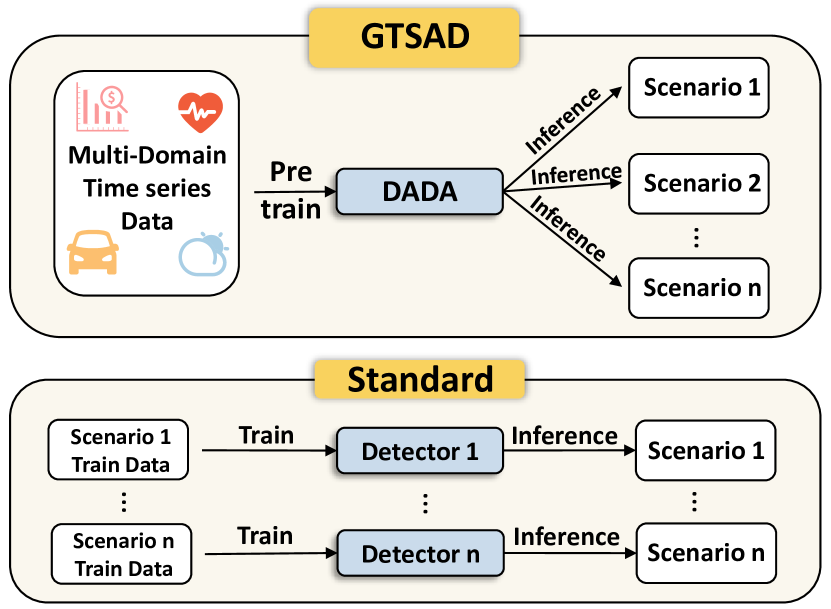
Figure 1: Illustration of general time series anomaly detection (GTSAD) and the standard methods.

in Figure 1, by pre-training the model on large time series data from multiple sources and domains, it is encouraged to learn anomaly detection from richer temporal information with cross-domain generalization capabilities. Then, the model can be efficiently applied to a wide range of downstream scenarios. However, constructing a general anomaly detection model still faces the following two major challenges.

First, the large-scale time series data are from multiple sources and domains with different information densities, which raises the challenge of meeting the diverse requirements of appropriate information bottlenecks tailored to different datasets in one unified model. Existing anomaly detection methods emphasize accurately capturing the characteristics of normal data with autoencoder, due to the inherently scarce nature of anomalies [17]. Information bottleneck is considered as a trade-off between compactly compressing the intrinsic information of the original data and high-fidelity reconstruction [18]. A large bottleneck can reconstruct the original data accurately but may cause the model to fit unnecessary noise unrelated to normal patterns. On the contrary, a small bottleneck can compactly compress the intrinsic information but may result in the loss of diverse normal patterns and poor reconstruction [13]. Existing anomaly detection methods typically tune a fixed internal information bottleneck for each scenario, which is limited in inflexible representation capability and insufficient generalization ability when facing multi-domain time series data with significantly different data distributions, periodicity, and noise levels [19], making it difficult to adapt well to downstream scenarios.

Second, the diverse manifestations of anomalies across multiple domains pose another significant challenge of robust distinguishment between normal patterns and diverse anomaly patterns. A model capable of general anomaly detection not only needs to have a clear understanding of normal patterns in time series data from different domains but also requires a clear delineation of decision boundaries between normal patterns and diverse abnormal patterns. Existing anomaly detection methods are often based on the one-class classification assumption and only learn normal patterns in time series data for each specific domain, lacking explicit differentiation of the anomalies. As a result, they may struggle to distinguish between normal and abnormal patterns for general time series, where multi-domain data exist with diverse anomaly manifestations and the decision boundaries between normal and abnormal patterns are more complex.

In this paper, we propose a novel general time series anomaly Detector with Adaptive bottlenecks and Dual Adversarial decoders (DADA). For the first challenge, we introduce the Adaptive Bottlenecks module to enhance the learning of normal time series patterns from multi-domain data. We employ a bottleneck to compress features into the latent space, the size of which can manifest different information densities for multi-domain data [13]. To meet the requirements of different information bottlenecks for divergent data, we establish a bottleneck pool containing various bottlenecks with different latent space sizes. Then, a data-adaptive mechanism is further proposed to enable the flexible selection of proper internal sizes based on the unique reconstruction requirements of the input data. To address the second challenge, we propose the Dual Adversarial Decoders module, which works with the encoder to enlarge the robust distinguishment between normal and anomaly patterns, where the normal decoder learns normal patterns for accurate reconstruction of normal sequences, and the anomaly decoder learns different anomaly patterns from anomaly time series separately. We design an adversarial training mechanism for the encoder and the anomaly decoder on the reconstruction of abnormal series, which learns explicit decision boundaries between normal and anomalies during the multi-domain training and thereby improves the anomaly detection capability across different scenarios. Our main contributions are summarized as follows:

• We propose DADA, a novel General Time Series Anomaly Detector with Adaptive Bottlenecks and Dual Adversarial Decoders. By pre-training on multi-domain time series data, we have achieved the goal of "one-model-for-many", meaning a single model can perform anomaly detection on various target scenarios, without requiring any fine-tuning on each downstream dataset.

• Technically, the novel Adaptive Bottlenecks addresses the flexible reconstruction requirements of multi-domain time series data and empowers the model’s generalization capability.

• The Dual Adversarial Decoders that explicitly amplify the decision boundaries between normal and anomalies improve the anomaly detection capability across different scenarios.

• Our model acts as a zero-shot time series anomaly detector that achieves competitive or superior performance on various downstream datasets, compared to state-of-the-art models trained for each specific dataset.

2 Related Work

Time series anomaly detection.

With the widespread application of various sensors, time series anomaly detection has gained widespread attention and can be categorized into none-learning, classical learning, and deep learning [20]. Non-learning methods include density-based methods [21, 22, 23, 24] that determine which data points are abnormal by analyzing the density of the distribution of data points in the cluster, and similarity-based methods [25] that series significantly dissimilar from most series are marked as abnormal. Classical learning methods [26] partition the time series into windows and use a training dataset consisting of only normal data to classify whether the test data is similar to the normal data or not [27]. Deep learning methods mainly contain reconstruction-based and prediction-based methods. The reconstruction-based methods compress the raw input data and then attempt to reconstruct this representation, the abnormal data is often difficult to reconstruct correctly [20]. This class of methods uses the difference between the reconstructed result and the original input as a criterion to determine the anomaly. The classic approaches include the use of AEs in  [14, 28], VAEs in  [11, 29, 30] or GANs in  [31, 32, 33], and more recently, the highly successful utilization of transformer architectures in [10, 15, 34]. The prediction-based methods [35] use past observations to predict the current value and use the difference between the predicted result and the real value as an anomaly criterion. Unlike these methods that require building a model for each dataset, our method mainly focuses on constructing a general time series anomaly detection model by pre-training on multi-domain time series data, which can be efficiently applied to various target datasets.

Time series pre-training models.

Time series pre-training models have received extensive attention. Some works have developed general pre-training strategies for time series data. PatchTST [36] and SimMTM [37] employ the BERT-style masked pretraining. InfoTS [38] and TS2Vec [39] utilize contrastive learning between augmented views of time series. Additionally, Some works repurpose large language models to time series tasks [40], such as GPT4TS [41]. Recently, novel time series pre-training models with zero-shot forecasting capabilities have emerged [42, 43, 19, 44, 45, 40], which demonstrate remarkable performance even without training on the target datasets. Nonetheless, there remains a dearth of time series anomaly detection models that support zero-shot. Existing pre-training methods for anomaly detection necessitate training on the target dataset. Different from previous methods, DADA pre-trained on multi-domain datasets is uniquely designed for time series anomaly detection, excelling in zero-shot anomaly detection across various target scenarios, thus filling this gap in the field.

3 Methodology

Given a time series $\mathcal{D}_{\text{test}}=\left(\mathbf{x}_{1},\mathbf{x}_{2},\cdots,\mathbf{x}_{T}\right)\in\mathbb{R}^{d\times T}$ containing $T$ successive observations, where $d$ is the data dimensions. Time series anomaly detection outputs $\mathcal{\hat{Y}}_{\text{text}}=\left(y_{1},y_{2}\cdots,y_{T}\right)$, where $y_{t}\in\{0,1\}$ denoting whether the observation $\mathbf{x}_{t}\in\mathbb{R}^{d}$ at a certain time $t$ is anomalous or not. In this paper, we focus on building a general time series anomaly detection model that is pre-trained on $M$ multi-domain time series datasets $\mathcal{D}=\{\mathcal{D}^{(i)}\}_{i=1}^{M}$, where each dataset $\mathcal{D}^{(i)}=\left(\mathbf{x}^{(i)}_{1},\mathbf{x}^{(i)}_{2},...,\mathbf{x}^{(i)}_{T^{(i)}}\right)\in\mathbb{R}^{d^{(i)}\times T^{(i)}}$ has $d^{(i)}\text{-variates}$ and $T^{(i)}$ time points. Then, the pre-trained model can be applied for anomaly detection on a target downstream dataset $\mathcal{D}_{\text{test}}\notin\mathcal{D}$ without any fine-tuning. Time series from different domains have varying numbers of variates. Thus, we use channel independence to extend our model across different domains [36, 15, 46, 45]. Specifically, a $d$-variate time series is processed into $d$ separate univariate time series.

3.1 Overall architecture

We propose DADA, a novel general time series anomaly Detector with Adaptive bottlenecks and Dual Adversarial decoders. As shown in Figure 2, DADA employs a mask-based reconstruction architecture to model time series. During the pre-training stage, we utilize normal series, where no time points are labeled as anomalies, and abnormal series, which contains labeled abnormal points. Both normal and abnormal time series are concurrently input to DADA. The patch and complementary mask module maps each series to masked patch embeddings, which are fed into the encoder to extract temporal features. DADA employs adaptive bottlenecks for multi-domain time series data by dynamically selecting suitable bottleneck sizes. Finally, the dual adversarial decoders are employed to reconstruct the normal and abnormal series. During the inference stage, the anomaly decoder is removed, and DADA employs multiple complementary masks to produce multiple pairs of masked patch embeddings. The variance of the reconstructed values serves as the anomaly score, where the normal data can be stably reconstructed.

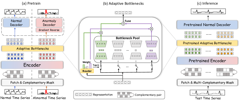
Figure 2: (a) The workflow during the pre-training stage. DADA mainly consists of Patch and Complementary Mask, Encoder, Adaptive Bottlenecks, and Dual Adversarial Decoders. (b) The structure of Adaptive Bottlenecks. (c) The workflow during the inference stage.

3.2 Complementary mask modeling

Time series mask modeling reconstructs masked parts using unmasked parts, to capture normal temporal dependencies from unmasked parts to masked parts. High reconstruction errors indicate anomalies that deviate from normal behavior. In this paper, We employ a complementary mask strategy by generating a pair of masked series with mutually complementary mask positions, which reconstruct each other to further capture comprehensive bi-directional temporal dependencies.

The complementary mask modeling consists of three steps. First, we split a univariate input time series into $P$ patches with patch size $S$, denoted as $\mathbf{X}\in\mathbb{R}^{P\times S}$. The division of time series data with patches has proven to be very helpful for capturing local information within each patch and learning global information among different patches, enabling the capture of complex temporal patterns [36, 15]. Then, we generate a masked series by randomly masking a portion of patches along the temporal dimension, formalized by $\mathbf{X}_{\text{m}}=\mathbf{M}\odot\mathbf{X}$, where $\mathbf{M}\in\{0,1\}^{P\times S}$ is the mask and $\odot$ is the element-wise multiplication. At the same time, we generate another masked time series that complements $\mathbf{X}_{\text{m}}$ according to the mask $\mathbf{M}$, formalized by $\mathbf{\bar{X}}_{\text{m}}=(1-\mathbf{M})\odot\mathbf{X}$. Then, we reconstruct the masked parts, $\mathbf{\bar{X}}_{\text{m}}$, based on $\mathbf{X}_{\text{m}}$, and vice versa. This provides the model fully utilizing all data points to capture comprehensive bi-directional temporal dependencies. Finally, we combine the complementary reconstructed results. Denoting the process of reconstruction as $\mathrm{Recon}(\cdot)$, the final reconstructed results $\mathbf{\hat{X}}$ is calculated by:

$$\mathbf{\hat{X}}=(1-\mathbf{M})\odot\mathrm{Recon}(\mathbf{X}_{\text{m}})+\mathbf{M}\odot\mathrm{Recon}(\mathbf{\bar{X}}_{\text{m}}).$$ (1)

In this paper, we employ this complementary mask reconstruction architecture to reconstruct normal and abnormal series respectively, leveraging the reconstruction outputs for model training and anomaly detection as detailed in Section 3.4.

3.3 Adaptive bottlenecks

As aforementioned, DADA is pre-trained on multi-domain time series datasets and applied to a wide range of downstream scenarios. This requires DADA to have the ability to learn generalizable representations from multi-domain time series datasets that show significant differences in data distribution, noise levels, etc. [43], and exhibit distinct preferences for the bottleneck. The size of the latent space can be considered as the internal information bottleneck of the model [13]. A large bottleneck may cause the model to fit unnecessary noise, while a small bottleneck may result in the loss of diverse normal patterns. The fixed bottleneck approaches used by existing methods [14, 11, 47] are poor in generalization ability and fail to detect anomalies across domains. Thus, we propose an innovative Adaptive Bottlenecks module (AdaBN) integrated with an adaptive router and a bottleneck pool, which dynamically allocates appropriate bottlenecks for multi-domain time series, enhancing the generalization ability of the model and enabling it to directly apply in various target scenarios.

Bottleneck pool.

We compress the features into different latent spaces to achieve different information bottlenecks with different information densities. To accommodate the varying requirements of the multi-domain time series data, we have configured a pool of $B$ different sizes of bottlenecks $\mathrm{BN}_{i}(\cdot),\ i=1,2,...,B$, and each of them can compress the features into a different-sized latent space with dimension $d_{i}$. The masked time series input encoder can generate the corresponding representation $\mathbf{z}\in\mathbb{R}^{d_{\text{r}}}$, where $d_{\text{r}}$ denotes the dimension of representation. The process of each bottleneck can be formalized as:

$$\mathrm{BN}_{i}(\mathbf{z})=\mathrm{UpNet}_{i}\left(\mathrm{DownNet}_{i}\left(\mathbf{z}\right)\right).$$ (2)

$\mathrm{DownNet}_{i}(\cdot)$ represents the network which compresses the representation $\mathbf{z}$ into a latent space, $\mathbb{R}^{d_{\text{r}}}\rightarrow\mathbb{R}^{d_{\text{i}}}$, where $d_{\text{i}}$ is the latent space dimension for the i-th bottleneck $\mathrm{BN}_{i}(\cdot)$ and $d_{\text{i}}<d_{\text{r}}$. $\mathrm{UpNet}_{i}(\cdot)$ restores the representation $\mathbf{z}$ from the latent space, $\mathbb{R}^{d_{\text{i}}}\rightarrow\mathbb{R}^{d_{\text{r}}}$.

Adaptive router.

Employing all bottlenecks within the bottleneck pool indiscriminately will diminish model performance due to the mismatching between the information capacity of the latent space and the information densities of the data. An ideal model would dynamically allocate appropriate bottlenecks based on the intrinsic properties of the time series data. Therefore, we introduce the Adaptive Router, a dynamic allocation strategy that can flexibly select bottleneck size for each time series. As shown in Figure 2(b), the adaptive router employs a routing function to generate the selecting weights of each bottleneck from the bottleneck pool based on the representation. To avoid repeatedly selecting certain bottlenecks, causing the corresponding bottlenecks to be repeatedly updated while neglecting other potentially suitable bottlenecks, we add noise terms to increase randomness. We obtain the overall formula for the routing function $\mathrm{R}(\mathbf{z})$ as:

$$\mathrm{R}(\mathbf{z})=\mathbf{z}\mathbf{W}_{\text{router}}+\epsilon\cdot\mathrm{Softplus}\left(\mathbf{z}\mathbf{W}_{\text{noise}}\right),\epsilon\sim\mathcal{N}\left(0,1\right),$$ (3)

where $\mathbf{W}_{\text{router}}$ and $\mathbf{W}_{\text{noise}}\in\mathbb{R}^{{d_{\text{r}}}\times B}$ are learnable matrices for weights generation, $B$ is the number of bottlenecks and $\mathrm{Softplus}$ is the activation function. $\mathrm{R}(\mathbf{z})$ maps representation $\mathbf{z}$ to selection weights for $B$ bottlenecks. To encourage the model to update key bottlenecks, we select $k$ bottlenecks with the highest weights, denoting the set of their indexes as $\mathcal{K}$. Last, we assign higher attention weights to the output of more important bottlenecks and fuse their final output as:

$$\mathrm{AdaBN}(\mathbf{z})=\sum_{i\in\mathcal{K}}\frac{\exp\left(\mathrm{R}\left(\mathbf{z}\right)_{i}\right)}{\sum_{j\in\mathcal{K}}\exp\left(\mathrm{R}\left(\mathbf{z}\right)_{j}\right)}\mathrm{BN}_{i}\left(\mathbf{z}\right).$$ (4)

3.4 Dual adversarial decoders

Reconstruction of normal time series.

As shown in Eq. (1), each input series $\mathbf{X}$ is reconstructed into result $\mathbf{\hat{X}}$. To achieve the goal of anomaly detection, we learn normal patterns from the reconstruction of normal time series. As shown in Figure 3, we use a feature extractor $G(\cdot;\theta_{g})$, and a normal decoder $D_{\text{n}}(\cdot;\theta_{n})$ with parameter $\theta_{g}$ and $\theta_{n}$ to denote the parts of the model used for reconstructing normal series. The $G$ includes the patch and complementary mask module, the encoder, and the adaptive bottlenecks. The decoder $D_{\text{n}}$ uses the output from the adaptive bottlenecks to reconstruct the series. We learn normal time series patterns by minimizing the reconstruction error of normal series:

$$\mathcal{L}_{\text{n}}(\theta_{g},\theta_{n})=\sum_{i=1}^{N_{\text{n}}}\|\mathbf{X}_{\text{n}}^{(i)}-\mathbf{\hat{X}}_{\text{n}}^{(i)}\|_{2}^{2}=\sum_{i=1}^{N_{\text{n}}}\|\mathbf{X}_{\text{n}}^{(i)}-D_{n}(G(\mathbf{X}_{\text{n}}^{(i)};\theta_{g});\theta_{n})\|_{2}^{2},$$ (5)

where $N_{\text{n}}$ is the number of normal training series. $\mathbf{X}_{\text{n}}^{(i)}$ is the $i\text{-th}$ normal series and $\mathbf{\hat{X}}_{\text{n}}^{(i)}$ is the corresponding reconstruction result.

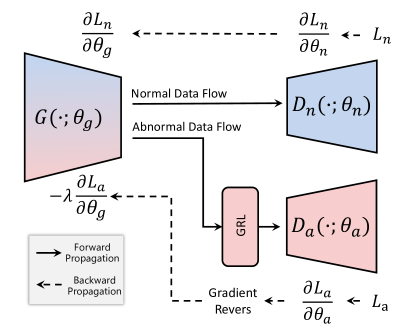
Figure 3: The forward and backward propagation of normal data and abnormal data.

Reconstruction of abnormal time series.

However, merely learning to capture normal patterns is insufficient to detect anomalies in new scenarios. As a general time series anomaly detection model, the model will confront multi-domain data with diverse anomaly manifestations, making the decision boundaries more complex. Thus, we need to explicitly enhance the model’s ability to discriminate between normal patterns and diverse abnormal patterns. We incorporate abnormal series into the pre-training stage and propose an adversarial training stage that minimizes reconstruction errors for normal series while maximizing them for abnormal ones. Simply amplifying the reconstruction error for anomalies can confuse the feature extractor $G$ and fail to learn normal patterns. To address this, we introduce an anomaly decoder $D_{\text{a}}(\cdot;\theta_{a})$ with parameter $\theta_{a}$ for adversarial training to constrain the model and encourage the feature extractor $G(\cdot;\theta_{g})$ to learn normal pattern features. We seek the parameters $\theta_{g}$ of the feature extractor that maximizes the reconstruction loss of the abnormal data to make the representations contain abnormal information as little as possible, while simultaneously seeking the parameters $\theta_{a}$ of the anomaly decoder that minimizes the reconstruction loss of the abnormal data to learn anomaly patterns. The reconstruction loss for abnormal series can be formalized as:

$$\mathcal{L}_{\text{a}}(\theta_{g},\theta_{a})=\sum_{i=1}^{N_{\text{a}}}\|\left(\mathbf{X}_{\text{a}}^{(i)}-\mathbf{\hat{X}}_{\text{a}}^{(i)}\right)\odot\mathbf{Y}_{\text{a}}^{(i)}\|_{2}^{2}=\sum_{i=1}^{N_{\text{a}}}\|\left(\mathbf{X}_{\text{a}}^{(i)}-D_{\text{a}}(G(\mathbf{X}_{\text{a}}^{(i)};\theta_{g});\theta_{a})\right)\odot\mathbf{Y}_{\text{a}}^{(i)}\|_{2}^{2},$$ (6)

where $N_{\text{a}}$ is the number of abnormal training series, $\mathbf{X}_{\text{a}}^{(i)}$ and $\mathbf{Y}_{\text{a}}^{(i)}$ denote the $i\text{-th}$ abnormal series and its anomaly label. Our method does not strictly require labeled data. In the absence of labeled abnormal series in the pre-training dataset, we can generate labeled abnormal series through the method of anomaly injection. More details about anomaly injection are shown in Appendix A.3.

Model training.

As aforementioned, the overall optimization goal is to seek the parameters $\theta_{g}$ of feature extractor that maximize Eq. (6), while simultaneously seeking the parameters $\theta_{a}$ of anomaly decoder that minimize Eq. (6). In addition, we seek to minimize Eq. (5). As shown in Figure 3, we employ a Gradient Reversal Layer (GRL) [48] between $G$ and ${D}_{\text{a}}$. GRL alters the gradient from $D_{\text{a}}$, multiplies it by $-\lambda$, and passes it to $G$, guiding parameters of different optimization objectives toward the desired direction for gradient descent, thereby avoiding the need for two separate optimizations. Finally, our objective can be formalized by:

$$(\theta_{g}^{*},\theta_{n}^{*}) =\arg\min_{\theta_{g},\theta_{n}}\mathcal{L}_{\text{n}}(\theta_{g},\theta_{n})-\mathcal{L}_{\text{a}}(\theta_{g},\theta_{a}),$$ (7)

$$\theta_{a}^{*} =\arg\min_{\theta_{a}}\mathcal{L}_{\text{a}}(\theta_{g},\theta_{a}).$$

Anomaly criterion.

During the inference stage, the model generates multiple pairs of complementary masked series for a single series and outputs multiple reconstructed series. Normal data points can be stably reconstructed, with the higher proximity of the reconstruction values. Conversely, reconstructions of abnormal data points are difficult and tend to be more unstable. Therefore, we utilize the variance of reconstructed values at the same time point as the anomaly score. Following existing works [13, 11], we run the SPOT [49] to get the threshold $\delta$, and a time point is marked as an anomaly if its anomaly score is larger than $\delta$.

4 Experiments

4.1 Experimental settings

Datasets.

We employ a subset of the Monash [50] data hub and 12 datasets [51, 52, 53, 54, 55, 56, 57, 58, 59] from anomaly detection task for pre-training. The pre-training datasets consist of approximately 400 million time points and intricately represent a wide range of domains. To demonstrate the effectiveness of our method, we evaluate five widely used benchmark datasets: SMD [60], MSL [61], SMAP [61], SWaT [62], PSM [63]. We also evaluate CICIDS, Creditcard, GECCO, SWAN, four datasets from the NeurIPS-TS competition [64]. None of the downstream datasets for evaluation are included in the pre-training datasets. More details about the pre-training and evaluation datasets are shown in Appendix A.

Baselines.

We compare our model with 17 baselines for comprehensive evaluations, including the linear transformation-based models: OCSVM [27], PCA [65]; the density estimation-based methods: HBOS [66], LOF [21]; the outlier-based methods: IForest [26], LODA [67]; the neural network-based models: AutoEncoder (AE) [47], DAGMM [68], LSTM [61], CAE-Ensemble [14], BeatGAN [31], OmniAnomaly (Omni) [11], Anomaly Transformer (A.T.) [10], DCdetector [15], D3R [13], GPT4TS [41], ModernTCN [12].

Metrics.

Many existing methods use point adjustments (PA) to adjust the detection result. However, recent works have demonstrated that PA can lead to faulty performance evaluations [69]. Even if only one point in an anomaly segment is correctly detected, PA will assume that the model has detected the entire segment correctly, which is unreasonable [13]. To overcome this problem, we use the affiliation-based F1-score (F1) [69], which has been widely used recently [13, 15]. This score takes into account the average directed distance between predicted anomalies and ground truth anomaly events to calculate affiliated precision (P) and recall (R). We also employed the AUC_ROC (AUC) metric [13, 14]. We adopt official implementations and follow the configuration guidelines suggested by the respective papers. More details are shown in the Appendix B. All results are in %. The best ones are in bold and the second ones are underlined.

Table 1: Results for five real-world datasets.

Dataset	SMD			MSL			SMAP			SWaT			PSM
Metric	P	R	F1	P	R	F1	P	R	F1	P	R	F1	P	R	F1
OCSVM	66.98	82.03	73.75	50.26	99.86	66.87	41.05	69.37	51.58	56.80	98.72	72.11	57.51	58.11	57.81
PCA	64.92	86.06	74.01	52.69	98.33	68.61	50.62	98.48	66.87	62.32	82.96	71.18	77.44	63.68	69.89
HBOS	60.34	64.11	62.17	59.25	83.32	69.25	41.54	66.17	51.04	54.49	91.35	68.26	78.45	29.82	43.21
LOF	57.69	99.10	72.92	49.89	72.18	59.00	47.92	82.86	60.72	53.20	96.73	68.65	53.90	99.91	70.02
IForest	71.94	94.27	81.61	53.87	94.58	68.65	41.12	68.91	51.51	53.03	99.95	69.30	69.66	88.79	78.07
LODA	66.09	84.37	74.12	57.79	95.65	72.05	51.51	100.00	68.00	56.30	70.34	62.54	62.22	87.38	72.69
AE	69.22	98.48	81.30	55.75	96.66	70.72	39.42	70.31	50.52	54.92	98.20	70.45	60.67	98.24	75.01
DAGMM	63.57	70.83	67.00	54.07	92.11	68.14	50.75	96.38	66.49	59.42	92.36	72.32	68.22	70.50	69.34
LSTM	60.12	84.77	70.35	58.82	14.68	23.49	55.25	27.70	36.90	49.99	82.11	62.15	57.06	95.92	71.55
BeatGAN	74.11	81.64	77.69	55.74	98.94	71.30	54.04	98.30	69.74	61.89	83.46	71.08	58.81	99.08	73.81
Omni	79.09	75.77	77.40	51.23	99.40	67.61	52.74	98.51	68.70	62.76	82.82	71.41	69.20	80.79	74.55
CAE-Ensemble	73.05	83.61	77.97	54.99	93.93	69.37	62.32	64.72	63.50	62.10	82.90	71.01	73.17	73.66	73.42
A.T.	54.08	97.07	66.42	51.04	95.36	66.49	56.91	96.69	71.65	53.63	98.27	69.39	54.26	82.18	65.37
DCdetector	50.93	95.57	66.45	55.94	95.53	70.56	53.12	98.37	68.99	53.25	98.12	69.03	54.72	86.36	66.99
D3R	64.87	97.93	78.02	66.85	90.83	77.02	61.76	92.55	74.09	60.14	97.57	74.39	73.32	88.71	80.29
ModernTCN	74.07	94.79	83.16	65.94	93.00	77.17	69.50	65.45	67.41	59.14	89.22	71.13	73.47	86.83	79.59
GPT4TS	73.33	95.97	83.13	64.86	95.43	77.23	63.52	90.56	74.67	56.84	91.46	70.11	73.61	91.13	81.44
DADA (zero shot)	76.50	94.54	84.57	68.70	91.51	78.48	65.85	88.25	75.42	61.59	94.59	74.60	74.31	92.11	82.26

4.2 Main results

We first evaluate our DADA on five real-world datasets. As shown in Table 1, compared to the baselines directly trained with full data in each specific dataset, DADA, as a zero-shot detector, achieves state-of-the-art results in all five datasets, which demonstrates that DADA learned a general detection ability from a wide range of pre-training data, with clear distinguishment between multiple normal and anomalous patterns. We also evaluate our DADA on the NeurIPS-TS benchmark in Table 2, compared with the five recent methods that perform well as shown in Table 1. We can observe that these baselines fail to achieve consistent good results across different datasets. However, benefiting from pre-training on large-scale data, DADA achieves the best or most competitive results on all datasets, including the NeurIPS-TS datasets which are rich in anomaly types [10, 15]. It demonstrates the superior adaptability of DADA for different anomaly detection scenarios. More evaluation details with AUC_ROC can be found in Appendix C.

Table 2: Overall results for the NeurIPS-TS datasets.

Dataset	CICIDS		Creditcard		GECCO		SWAN
Metric	F1	AUC	F1	AUC	F1	AUC	F1	AUC
A.T.	34.71	49.00	65.14	52.55	64.27	51.60	33.67	44.74
DCdetector	40.02	53.95	58.28	42.36	66.18	45.38	14.42	43.48
D3R	67.79	41.99	72.03	93.59	91.83	80.72	43.19	37.31
ModernTCN	51.74	65.33	73.80	95.55	90.18	95.95	46.45	52.63
GPT4TS	54.00	67.91	72.88	95.58	88.11	90.21	47.27	51.93
DADA (zero shot)	73.49	69.33	75.12	95.73	90.20	93.44	71.93	53.29

Ablation study.

We further delved into the impact of individual components on the performance of DADA, as shown in Table 3. Firstly, we explore the impact of the AdaBN module. The first line results use a single fixed bottleneck for multi-domain datasets, eliminating the adaptive selection for various bottlenecks. When we removed the AdaBN module, the outcomes exhibited a decline of 5.04%. This emphasizes the criticality of selecting bottlenecks for different domains. Then, We also examine the influence of the dual adversarial decoders and its adversarial mechanism. The second line results directly maximize the reconstruction error of abnormal data, removing the adversarial mechanism. The third line results use a single decoder to reconstruct normal time series and abnormal time series, and the fourth line results simultaneously remove the adversarial mechanism and use a single decoder. We observe degradation in performance of w/o Adversarial by 16.26% (79.49%$\to$63.23%) compared with DADA, and 7.89% (71.17%$\to$63.23%) compared with the fifth line results suggesting that directly maximizing abnormal time series increases confusion and the need for confrontation with the feature extractor. Additionally, employing a single decoder to handle both normal and abnormal time series causes zero-shot performance to degrade, instructing the necessity of dual decoders.

Table 3: Ablation studies. We study the influence of adaptive bottlenecks, adversarial training, and dual decoders. All results are in %, and the best ones are in bold.

Dataset			SMD			MSL			SMAP			Avg
AdaBN	Adversarial	Dual Decoders	P	R	F1	P	R	F1	P	R	F1	F1
✗	✓	✓	71.13	93.61	80.84	62.79	91.74	74.55	58.91	84.10	69.29	74.45
✓	✗	✓	69.46	55.32	61.59	49.89	88.57	63.83	52.62	82.59	64.28	63.23
✓	✓	✗	75.77	87.82	81.35	64.82	84.32	73.29	61.50	80.27	69.64	74.76
✓	✗	✗	77.82	89.95	83.44	67.54	88.56	76.63	65.65	83.09	73.34	77.81
✗	✗	✗	78.60	74.96	76.74	65.20	72.69	68.74	55.22	88.57	68.03	71.17
✓	✓	✓	76.50	94.54	84.57	68.7	91.51	78.48	65.85	88.25	75.42	79.49

4.3 Model analysis

We analyze the effectiveness of adaptive bottlenecks and multi-domain pre-training and visualize the anomaly scores. We conducted additional analytical experiments, and the results are presented in Appendix D and Appendix E.

Analysis on adaptive bottlenecks.

To validate the effectiveness of AdaBN, we remove the AdaBN module and instead employ a fixed bottleneck size. As shown in Figure 4(left), we observe that different bottleneck sizes exhibit different preferences for various downstream scenarios, while also introducing notable drawbacks in certain scenarios, e.g. the model with a bottleneck size of 32 achieves 74.81% on Creditcard, whereas only 67.56% on MSL. However, DADA, with adaptive bottlenecks dynamically allocating appropriate bottlenecks, consistently outperforms models utilizing a single bottleneck, which further substantiates the efficacy of our method. We also visualize the proportion of different adaptive bottleneck sizes that each dataset selects in Appendix E.2

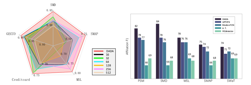
Figure 4: Model Analysis. (left) Comparison between DADA using AdaBN and using a single bottleneck. (right) Pre-training baseline model on multi-domain datasets and then evaluate them as a zero-shot detector on the target dataset.

Analysis on multi-domain pre-training.

We further evaluate the baseline’s zero-shot performance after multi-domain pre-training. Adopting the same setting as DADA, these models are first pre-trained extensively on multi-domain datasets, followed by zero-shot evaluation on the target datasets. From the presented Figure 4(right), we can observe that these baselines are incapable of effectively extracting generalization capability and robust distinguishment between normal patterns and diverse anomaly patterns from multi-domain datasets, thus failing to deliver satisfactory results on the target dataset. In contrast, DADA, equipped with its unique adaptive bottlenecks and dual adversarial decoders module tailored for the task of general anomaly detection, demonstrates great multi-domain pre-training and general detection ability.

Visual analysis.

To further explain the efficacy of each module within DADA, we randomly sample time segments of length 100 data points from all datasets for visualization. Figure 5 illustrates the anomaly scores at every timestamp within a given period and ground truth labels. After DADA removed the AdaBN module (W/O AdaBN), the model could not adapt well to the normal pattern of multi-domain data and got a higher false positive. After removing the dual decoders (W/O Dual Decoders), the model’s decision boundary between normal and abnormal data becomes blurred and the false negative becomes higher. DADA (ours) shows that DADA not only achieves superior detection accuracy but also maintains a lower false alarm rate, a testament to its refined performance in time series anomaly detection.

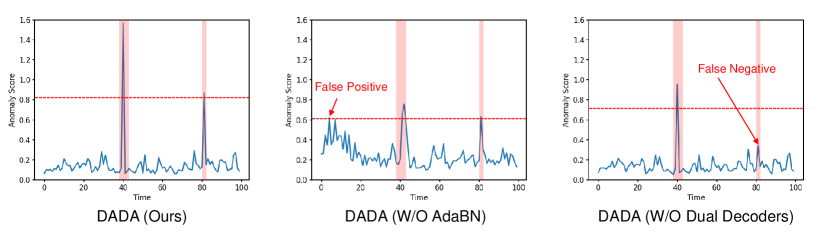
Figure 5: Visualization of the anomaly scores. The pink intervals denote the ground truth anomalies, while the blue lines represent the anomaly scores produced by corresponding models. A red horizontal dashed line signifies the threshold. Any timestamp with an anomaly score exceeding this threshold is identified as an anomaly.

5 Conclusion

This paper proposes a novel general time series anomaly detection model DADA. By pre-training on extensive multi-domain datasets, DADA can subsequently apply to a multitude of downstream scenarios without fine-tuning. We propose adaptive bottlenecks to meet the diverse requirements of information bottlenecks tailored to different datasets in one unified model. We also propose dual adversarial decoders to explicitly enhance clear differentiation between normal and abnormal patterns. Extensive experiments prove that as a zero-shot detector, DADA still achieves competitive or even superior results compared to those models tailored to each specific dataset.

Appendix A Datasets

A.1 Datasets for evaluation

We evaluate DADA and baselines on various datasets come from different domains, which can be broadly divided into spacecraft, servers, water treatment, finance, networking, and space weather:(1) SMD (Server Machine Dataset) collects resource utilization of computer clusters from an Internet company [60]. (2) MSL (Mars Science Laboratory dataset), collected by NASA, encompasses telemetry data reflecting the operational status of both sensors and actuators aboard the Martian rover [61]. (3) SMAP (Soil Moisture Active Passive dataset) is also collected by NASA and reflects soil moisture data from spacecraft monitoring systems [61]. (4) SWaT (Secure Water Treatment) collects sensor data from a continuously operating infrastructure [62]. (5) PSM (Pooled Server Metrics dataset) is collected from eBay Server Machines [63]. (6) NeurIPS-TS (NeurIPS 2021 Time Series Benchmark) is a dataset proposed by  [64] and we use four sub-datasets: CICIDS, Creditcard, GECCO, SWAN with a variety of anomaly scenarios. For MSL and SMAP datasets, we only retain the first continuous dimension [13]. We summarize the datasets in Table 4.

Table 4: Details of benchmark datasets for evaluation. AR (anomaly ratio) represents the abnormal proportion of the whole dataset.

Dataset	Domain	Dimension	Training	Validation	Test(labeled)	AR(%)
MSL	Spacecraft	55	46,653	11,664	73,729	10.5
PSM	Server Machine	25	105,984	26,497	87,841	27.8
SMAP	Spacecraft	25	108,146	27,037	427,617	12.8
SMD	Server Machine	38	566,724	141,681	708,420	4.2
SWAT	Water treatment	51	396,000	99,000	449,919	12.1
Creditcard	Finance	29	113,922	28,481	142,404	0.17
GECCO	Water treatment	9	55,408	13,852	69,261	1.25
CICIDS	Web	72	68,092	17,023	85,116	1.28
SWAN	Space Weather	38	48,000	12,000	60,000	23.8

A.2 Datasets for pre-training

We collect two datasets for pre-training, namely Anomaly Detection Data and $\text{Monash}^{+}$, each of them contains normal time series and abnormal time series. None of the downstream datasets for evaluation are included in the pre-training datasets. Firstly, we collect the Anomaly Detection Data from time series anomaly detection task. Table 5 lists subsets in Anomaly Detection Data, including ASD [51], Exathlon [52], ECG [57], MITDB [57], OPP [54], SVDB [58], GAIA, IOPS [53], MGAB [56], NYC [55], SKAB, YAHOO [59]. In the field of time series anomaly detection, datasets usually contain default normal training data and labeled test data with anomalies. We take the training data of this part as normal data, and the data with anomaly labels in test data as abnormal data.

Table 5: Anomaly Detection Data selected from multi-domain time series anomaly detection task. AR (anomaly ratio) represents the abnormal proportion of the whole dataset.

Dataset	Domain	Dimension	Length	AR(%)
ASD	Application Server	19	384,493	1.55
Exathlon	Application Server	multi	131,610	8.71
ECG	Health	1	9,681,300	4.7
MITDB	Health	1	13,650,000	3.44
OPP	Health	1	14,567,752	4.11
SVDB	Health	1	17,049,600	4.68
GAIA	AIOps	1	1,868,506	1.21
IOPS	Web	1	5,840,488	2.15
MGAB	Mackey-Glass	1	1,000,000	0.2
NYC	Transport	3	17,520	0.57
SKAB	Machinery	8	46,707	3.65
YAHOO	Multiple	1	565,827	0.62

To further enlarge our pre-training data, we build the $\text{Monash}^{+}$ dataset. The normal time series in $\text{Monash}^{+}$ comes from the Monash Prediction Library [50] as shown in Table 6, and the abnormal time series in $\text{Monash}^{+}$ are generated from Monash by anomaly injection. The anomaly injection is shown in Figure 6. These time series with different variate numbers and series lengths from multi-domains reflect the diverse application of the real world and the overall pre-training datasets are summarized in Table 7.

Table 6: Multi-domain time series datasets from the Monash Prediction Library.

Dataset	Domain	frequency	Length
Aus. Electricity Demand	Energy	Half Hourly	1,155,264
Wind	Energy	4 Seconds	7,397,147
Wind Farms	Energy	Minutely	172,178,060
Solar Power	Energy	4Seconds	7,397,223
Solar	Energy	10 Minutes	7,200,857
London Smart Meters	Energy	Half Hourly	166,527,216
Saugeen River Flow	Nature	Daily	23,741
Sunspot	Nature	Daily	73,924
Weather	Nature	Daily	43,032,000
KDD Cup 2018	Nature	Daily	2,942,364
US Births	Nature	Daily	7,305
FRED_MD	Economic	Monthly	77,896
Bitcoin	Economic	Daily	75,364
NN5	Economic	Daily	87,801

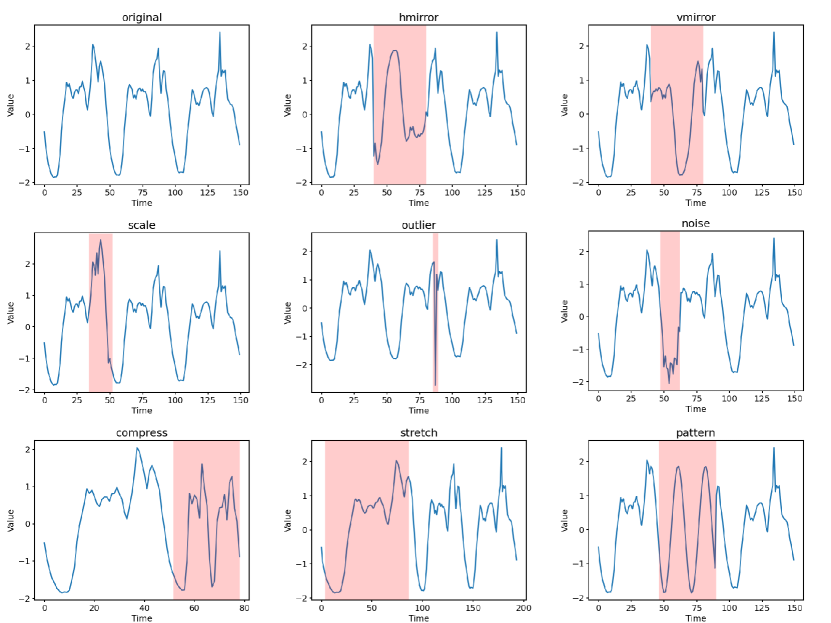
Figure 6: Anomaly injection. The blue lines represent the time series, while the pink areas intervals the anomalies we generated. We visualize the original time series and eight types of anomaly, including hmirror, vmirror, scale, outlier, noise, compress, stretch, and pattern.

A.3 Abnormal injection

We use abnormal time series in the pre-training to explicitly enable robust distinguishment between normal and abnormal patterns with our dual adversarial decoders. Due to the scarcity of labeled data in the field of time series anomaly detection, we enrich abnormal samples by abnormal injection on Monash. Utilizing methods such as vmirror, hmirror, compression, stretching, scaling, and others, as shown in Figure 6, we generate an expanded collection of novel time series exhibiting diverse anomaly types and patterns, thereby enhancing our model’s ability to distinguish between normal and abnormal time series.

Table 7: Description of pre-training datasets with normal data and abnormal data.

Dataset	Normal Time Series	Abnormal Time Series
Anomaly Detection Data	Training set	Test set
$\text{Monash}^{+}$	All of Moansh data	Generated from Monash by anomaly injection

Appendix B Implementation details

We summarize all the default hyper-parameters as follows. We use a dilated CNN as an encoder with ten layers [39]. In the implementation phase, we run a sliding window with a window size of 100 and conduct anomaly detection using non-overlapping windows the same as existing works [10, 11]. Our patch size is 5. The bottleneck pool contains the sizes [16, 32, 64, 128, 192, 256] and the adaptive router selects $k=3$ bottlenecks with the highest weights. The AdamW optimizer with an initial learning rate of $10^{-4}$ is used in pre-training. We set the batch size to 2048 with 5 epochs in pre-training, while each epoch costs approximately 1.5 hours. In the inference stage, we use 5 pairs of complementary masked series. After obtaining the anomaly score, we adopt commonly used SPOT [49] following existing works [13, 11] to get the threshold $\delta$ to determine whether each point is an outlier [13]. We conduct all experiments using Pytorch with NVIDIA Tesla-A800-80GB GPU.

Appendix C Additional detection result

We present supplementary results for the Area under the Receiver Operating Characteristic curve (AUC_ROC). AUC_ROC serves as a robust evaluation tool, allowing for an assessment of model performance across different thresholds. As shown in Table 8, we compare with the five recent methods that performed well in Table 1. As a zero-shot detector, DADA, consistently demonstrates comparable or superior performance to the state-of-the-art model, with an average improvement of 3.03%.

Table 8: AUC_ROC score results in the five real-world datasets. A higher AUC_ROC represents better performance. The best ones are in bold.

Dataset	SMD	MSL	SMAP	SWaT	PSM	Avg
Metric	AUC_ROC	AUC_ROC	AUC_ROC	AUC_ROC	AUC_ROC	AUC_ROC
A.T.	50.02	34.05	50.24	56.3	50.11	48.14
DC	49.82	36.61	43.68	51.80	50.20	46.42
D3R	53.34	45.77	44.90	81.59	50.22	55.16
ModernTCN	70.21	74.96	51.45	70.11	58.46	65.04
GPT4TS	71.15	72.63	52.06	22.92	58.94	55.54
DADA (zero shot)	71.98	75.15	51.23	80.90	61.08	68.07

Appendix D Parameter sensitivity

We study the parameter sensitivity of the DADA. Figure 7 shows the model performance under different window sizes, $k$ bottlenecks with the highest weights that the adaptive router can select, and different patch sizes. Window size is a very important parameter for time series analysis. In a time series, a single point does not contain any information, so the window size determines the length of the sample context. Our experiments show that DADA is insensitive to window size and performs well across different window sizes. We then explore the influence of parameter $k$ in the adaptive bottlenecks. From the performance point of view, our model shows a relatively stable effect under different $k$, where we can achieve good performance even when selecting 1 bottleneck for each sample. Finally, we study the performance under different patch sizes. Patch splitting has proven to be very helpful for capturing local information within each patch and learning global information among different patches. The results in Figure 7 show that DADA is robust under different patch sizes.

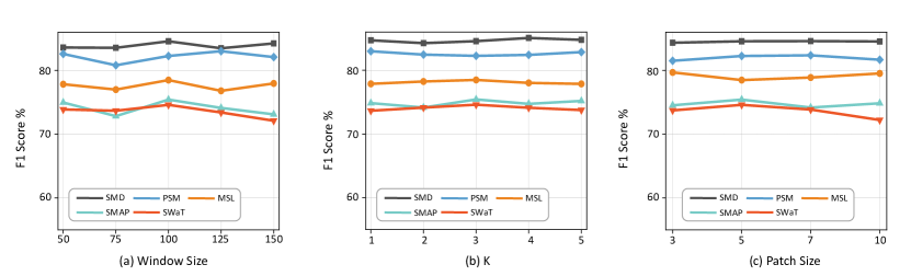
Figure 7: (a) Parameter sensitivity for sliding window size, (b) $k$ bottlenecks with the highest weights that the adaptive router can select, and (c) patch sizes (c).

Appendix E Additional model analysis

E.1 Comparison with MoE

Mixture-of-Experts (MoE) [70] includes the gating network and multiple experts, each with the same structure. The gating network assigns different experts according to the characteristics of the data. In our AdaBN, each bottleneck in the bottleneck pool has a different hidden dimension. Each bottleneck compresses time series representation to a different hidden space to accommodate the varying requirements of the multi-domain time series data. As shown in table 9, to compare DADA with MoE, we replace all bottlenecks in the bottleneck pool with a consistent size of 256, which performs better compared to other hidden dimensions as shown in Figure 4. The results indicate that the improvement in our model’s performance is not just due to a larger number of parameters and more experts, but more crucially, to the special design of the bottleneck, adapted to the unique demands of general anomaly detection modeling.

Table 9: Comparison of DADA and MoE. Single 256 replaces the AdaBN with a single bottleneck with size 256. The MoE 256 changes all bottlenecks in the bottleneck pool to the same size 256. The result is reported with Affiliated F1, and the best ones are in bold.

Dataset	SMD	SMAP	MSL	SWaT	PSM
Metric	F1	F1	F1	F1	F1
single 256	81.69	74.37	77.01	69.93	80.15
MoE 256	84.25	74.87	78.41	71.68	81.69
DADA	84.57	75.42	78.48	74.60	82.26

E.2 Visualization of adaptive bottlenecks

As shown in Figure 8, our visualization illustrates the proportion of different adaptive bottleneck sizes that each dataset selects and prefers. The figure highlights distinct preferences among datasets, indicating variability in their selection criteria. Notably, the SMAP and MSL datasets, sourced from NASA spacecraft monitoring systems, display a similarity in their data characteristics. This observation is further supported by our experimental results in Figure 8, showcasing consistent preferences for bottleneck sizes within these datasets.

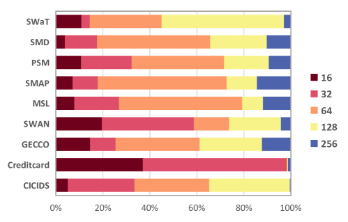
Figure 8: Visualization of the proportion of different bottleneck sizes that each dataset prefers.

E.3 Pre-training with multi-domain datasets

We investigated the impact of the pre-training datasets on our model’s performance. As depicted in Figure 9, we employ the $\text{Monash}^{+}$ in Table 6 and Anomaly Detection Data in Table 5 individually for pre-training, followed by zero-shot evaluation on the SMD, MSL, SMAP, SWaT, and PSM datasets. Our model consistently exhibits great performance with different pre-training datasets.

Furthermore, using both datasets together to expand the domain scope of pre-training datasets enhances the breadth of information assimilated by our adaptive bottlenecks and dual adversarial decoders. Consequently, this enrichment contributes to further improvements in model performance.

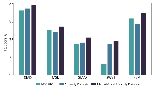
Figure 9: Pre-training with multi-domain datasets.

Appendix F Limitations and broader impacts

Time series anomaly detection is important in many application scenarios. Effectively detecting anomalies in time series data helps to identify potential issues in time and takes necessary measures to ensure the normal operation of systems, thereby avoiding possible economic losses and security threats. This is very beneficial to the development of social economy and urban security. Additionally, our model is a general time series anomaly detector with well zero-shot capability, which solves the problem of lack of training data of target scenario due to user privacy, time, labor costs and so on.

One limitation of our model is that we use channel independence for multivariate time series and do not design other special mechanisms for the modeling of the correlation between different time series variables, which may help better anomaly detection in some cases. We would like to leave this as a future work to explore how to capture such correlations under multi-domain pre-training situations. Besides, we mainly use CNNs as the backbone of our model, and we are also willing to explore our model with more other backbones such as RNNs and Transformers.

References

- Anandakrishnan et al. [2017] Archana Anandakrishnan, Senthil Kumar, Alexander R. Statnikov, Tanveer A. Faruquie, and Di Xu. Anomaly detection in finance: Editors’ introduction. In ADF@KDD, 2017.
- Cook et al. [2020] Andrew A. Cook, Goksel Misirli, and Zhong Fan. Anomaly detection for iot time-series data: A survey. IEEE Internet Things J., 2020.
- Kieu et al. [2022] Tung Kieu, Bin Yang, Chenjuan Guo, Razvan-Gabriel Cirstea, Yan Zhao, Yale Song, and Christian S. Jensen. Anomaly detection in time series with robust variational quasi-recurrent autoencoders. In ICDE, 2022.
- Yang et al. [2021] Yiyuan Yang, Haifeng Zhang, and Yi Li. Pipeline safety early warning by multifeature-fusion CNN and lightgbm analysis of signals from distributed optical fiber sensors. IEEE Trans. Instrum. Meas., 2021.
- Dong et al. [2023a] Feng Dong, Liu Wang, Xu Nie, Fei Shao, Haoyu Wang, Ding Li, Xiapu Luo, and Xusheng Xiao. DISTDET: A cost-effective distributed cyber threat detection system. In USENIX Security Symposium, 2023a.
- Wang and Zhu [2022] Cheng Wang and Hangyu Zhu. Wrongdoing monitor: A graph-based behavioral anomaly detection in cyber security. IEEE Trans. Inf. Forensics Secur., 2022.
- Li et al. [2022] Zhuozhao Li, Tanmoy Sen, Haiying Shen, and Mooi Choo Chuah. A study on the impact of memory dos attacks on cloud applications and exploring real-time detection schemes. IEEE/ACM Trans. Netw., 2022.
- Wang et al. [2023a] Huazhang Wang, Zhaojing Luo, James Wei Luen Yip, Chuyang Ye, and Meihui Zhang. ECGGAN: A framework for effective and interpretable electrocardiogram anomaly detection. In KDD, 2023a.
- Salem et al. [2021] Osman Salem, Khalid Alsubhi, Ahmed Mehaoua, and Raouf Boutaba. Markov models for anomaly detection in wireless body area networks for secure health monitoring. IEEE J. Sel. Areas Commun., 2021.
- Xu et al. [2022] Jiehui Xu, Haixu Wu, Jianmin Wang, and Mingsheng Long. Anomaly transformer: Time series anomaly detection with association discrepancy. In ICLR, 2022.
- Su et al. [2019a] Ya Su, Youjian Zhao, Chenhao Niu, Rong Liu, Wei Sun, and Dan Pei. Robust anomaly detection for multivariate time series through stochastic recurrent neural network. In KDD, 2019a.
- donghao and wang xue [2024] Luo donghao and wang xue. ModernTCN: A modern pure convolution structure for general time series analysis. In ICLR, 2024.
- Wang et al. [2023b] Chengsen Wang, Zirui Zhuang, Qi Qi, Jingyu Wang, Xingyu Wang, Haifeng Sun, and Jianxin Liao. Drift doesn’t matter: Dynamic decomposition with diffusion reconstruction for unstable multivariate time series anomaly detection. In NeurIPS, 2023b.
- Campos et al. [2021] David Campos, Tung Kieu, Chenjuan Guo, Feiteng Huang, Kai Zheng, Bin Yang, and Christian S. Jensen. Unsupervised time series outlier detection with diversity-driven convolutional ensembles - extended version. CoRR, 2021.
- Yang et al. [2023] Yiyuan Yang, Chaoli Zhang, Tian Zhou, Qingsong Wen, and Liang Sun. Dcdetector: Dual attention contrastive representation learning for time series anomaly detection. In KDD, 2023.
- Zhang et al. [2023] Kexin Zhang, Qingsong Wen, Chaoli Zhang, Rongyao Cai, Ming Jin, Yong Liu, James Zhang, Yuxuan Liang, Guansong Pang, Dongjin Song, and Shirui Pan. Self-supervised learning for time series analysis: Taxonomy, progress, and prospects. CoRR, 2023.
- Chalapathy and Chawla [2019] Raghavendra Chalapathy and Sanjay Chawla. Deep learning for anomaly detection: A survey. CoRR, 2019.
- Kawaguchi et al. [2023] Kenji Kawaguchi, Zhun Deng, Xu Ji, and Jiaoyang Huang. How does information bottleneck help deep learning? In ICML, 2023.
- Liu et al. [2024a] Xu Liu, Junfeng Hu, Yuan Li, Shizhe Diao, Yuxuan Liang, Bryan Hooi, and Roger Zimmermann. Unitime: A language-empowered unified model for cross-domain time series forecasting. In WWW, 2024a.
- Zhao et al. [2022] Yan Zhao, Liwei Deng, Xuanhao Chen, Chenjuan Guo, Bin Yang, Tung Kieu, Feiteng Huang, Torben Bach Pedersen, Kai Zheng, and Christian S. Jensen. A comparative study on unsupervised anomaly detection for time series: Experiments and analysis. CoRR, 2022.
- Breunig et al. [2000] Markus M. Breunig, Hans-Peter Kriegel, Raymond T. Ng, and Jörg Sander. LOF: identifying density-based local outliers. In SIGMOD Conference, 2000.
- Kriegel et al. [2009] Hans-Peter Kriegel, Peer Kröger, Erich Schubert, and Arthur Zimek. Loop: local outlier probabilities. In CIKM, 2009.
- Tang et al. [2002a] Jian Tang, Zhixiang Chen, Ada Fu, and David Cheung. A robust outlier detection scheme for large data sets. Proc. Pacific-Asia Conf. Knowledge Discovery and Data Mining, 01 2002a.
- Tang et al. [2002b] Jian Tang, Zhixiang Chen, Ada Wai-Chee Fu, and David Wai-Lok Cheung. Enhancing effectiveness of outlier detections for low density patterns. In PAKDD, 2002b.
- Yeh et al. [2016] Chin-Chia Michael Yeh, Yan Zhu, Liudmila Ulanova, Nurjahan Begum, Yifei Ding, Hoang Anh Dau, Diego Furtado Silva, Abdullah Mueen, and Eamonn J. Keogh. Matrix profile I: all pairs similarity joins for time series: A unifying view that includes motifs, discords and shapelets. In ICDM, 2016.
- Liu et al. [2008] Fei Tony Liu, Kai Ming Ting, and Zhi-Hua Zhou. Isolation forest. In ICDM, 2008.
- Schölkopf et al. [1999] Bernhard Schölkopf, Robert C. Williamson, Alexander J. Smola, John Shawe-Taylor, and John C. Platt. Support vector method for novelty detection. In NIPS, 1999.
- Krizhevsky et al. [2012] Alex Krizhevsky, Ilya Sutskever, and Geoffrey E. Hinton. Imagenet classification with deep convolutional neural networks. In NIPS, 2012.
- Park et al. [2018] Daehyung Park, Yuuna Hoshi, and Charles C. Kemp. A multimodal anomaly detector for robot-assisted feeding using an lstm-based variational autoencoder. IEEE Robotics Autom. Lett., 2018.
- Li et al. [2021a] Zhihan Li, Youjian Zhao, Jiaqi Han, Ya Su, Rui Jiao, Xidao Wen, and Dan Pei. Multivariate time series anomaly detection and interpretation using hierarchical inter-metric and temporal embedding. In KDD, 2021a.
- Zhou et al. [2019] Bin Zhou, Shenghua Liu, Bryan Hooi, Xueqi Cheng, and Jing Ye. Beatgan: Anomalous rhythm detection using adversarially generated time series. In IJCAI, 2019.
- Li et al. [2019] Dan Li, Dacheng Chen, Baihong Jin, Lei Shi, Jonathan Goh, and See-Kiong Ng. MAD-GAN: multivariate anomaly detection for time series data with generative adversarial networks. In ICANN (4), 2019.
- Schlegl et al. [2019] Thomas Schlegl, Philipp Seeböck, Sebastian M. Waldstein, Georg Langs, and Ursula Schmidt-Erfurth. f-anogan: Fast unsupervised anomaly detection with generative adversarial networks. Medical Image Anal., 2019.
- Chen et al. [2022] Zekai Chen, Dingshuo Chen, Xiao Zhang, Zixuan Yuan, and Xiuzhen Cheng. Learning graph structures with transformer for multivariate time-series anomaly detection in iot. IEEE Internet Things J., 2022.
- Pang et al. [2022] Guansong Pang, Chunhua Shen, Longbing Cao, and Anton van den Hengel. Deep learning for anomaly detection: A review. ACM Comput. Surv., 2022.
- Nie et al. [2023] Yuqi Nie, Nam H. Nguyen, Phanwadee Sinthong, and Jayant Kalagnanam. A time series is worth 64 words: Long-term forecasting with transformers. In ICLR, 2023.
- Dong et al. [2023b] Jiaxiang Dong, Haixu Wu, Haoran Zhang, Li Zhang, Jianmin Wang, and Mingsheng Long. Simmtm: A simple pre-training framework for masked time-series modeling. In NeurIPS, 2023b.
- Luo et al. [2023] Dongsheng Luo, Wei Cheng, Yingheng Wang, Dongkuan Xu, Jingchao Ni, Wenchao Yu, Xuchao Zhang, Yanchi Liu, Yuncong Chen, Haifeng Chen, and Xiang Zhang. Time series contrastive learning with information-aware augmentations. In AAAI, 2023.
- Yue et al. [2022] Zhihan Yue, Yujing Wang, Juanyong Duan, Tianmeng Yang, Congrui Huang, Yunhai Tong, and Bixiong Xu. Ts2vec: Towards universal representation of time series. In AAAI, 2022.
- Gruver et al. [2023] Nate Gruver, Marc Finzi, Shikai Qiu, and Andrew Gordon Wilson. Large language models are zero-shot time series forecasters. In NeurIPS, 2023.
- Zhou et al. [2023] Tian Zhou, Peisong Niu, Xue Wang, Liang Sun, and Rong Jin. One fits all: Power general time series analysis by pretrained LM. In NeurIPS, 2023.
- Garza and Canseco [2023] Azul Garza and Max Mergenthaler Canseco. Timegpt-1. CoRR, 2023.
- Woo et al. [2024] Gerald Woo, Chenghao Liu, Akshat Kumar, Caiming Xiong, Silvio Savarese, and Doyen Sahoo. Unified training of universal time series forecasting transformers. CoRR, 2024.
- Dooley et al. [2023] Samuel Dooley, Gurnoor Singh Khurana, Chirag Mohapatra, Siddartha V. Naidu, and Colin White. Forecastpfn: Synthetically-trained zero-shot forecasting. In NeurIPS, 2023.
- Liu et al. [2024b] Yong Liu, Haoran Zhang, Chenyu Li, Xiangdong Huang, Jianmin Wang, and Mingsheng Long. Timer: Transformers for time series analysis at scale. CoRR, 2024b.
- Goswami et al. [2024] Mononito Goswami, Konrad Szafer, Arjun Choudhry, Yifu Cai, Shuo Li, and Artur Dubrawski. MOMENT: A family of open time-series foundation models. In ICML, 2024.
- Sakurada and Yairi [2014] Mayu Sakurada and Takehisa Yairi. Anomaly detection using autoencoders with nonlinear dimensionality reduction. In MLSDA@PRICAI, 2014.
- Ganin and Lempitsky [2015] Yaroslav Ganin and Victor S. Lempitsky. Unsupervised domain adaptation by backpropagation. In ICML, 2015.
- Siffer et al. [2017] Alban Siffer, Pierre-Alain Fouque, Alexandre Termier, and Christine Largouët. Anomaly detection in streams with extreme value theory. In KDD, 2017.
- Godahewa et al. [2021] Rakshitha Godahewa, Christoph Bergmeir, Geoffrey I. Webb, Rob J. Hyndman, and Pablo Montero-Manso. Monash time series forecasting archive. In NeurIPS Datasets and Benchmarks, 2021.
- Li et al. [2021b] Zhihan Li, Youjian Zhao, Jiaqi Han, Ya Su, Rui Jiao, Xidao Wen, and Dan Pei. Multivariate time series anomaly detection and interpretation using hierarchical inter-metric and temporal embedding. In KDD, 2021b.
- Jacob et al. [2021] Vincent Jacob, Fei Song, Arnaud Stiegler, Bijan Rad, Yanlei Diao, and Nesime Tatbul. Exathlon: A benchmark for explainable anomaly detection over time series. Proc. VLDB Endow., 2021.
- Ren et al. [2019] Hansheng Ren, Bixiong Xu, Yujing Wang, Chao Yi, Congrui Huang, Xiaoyu Kou, Tony Xing, Mao Yang, Jie Tong, and Qi Zhang. Time-series anomaly detection service at microsoft. In KDD, 2019.
- Roggen et al. [2010] Daniel Roggen, Alberto Calatroni, Mirco Rossi, Thomas Holleczek, Kilian Förster, Gerhard Tröster, Paul Lukowicz, David Bannach, Gerald Pirkl, Alois Ferscha, Jakob Doppler, Clemens Holzmann, Marc Kurz, Gerald Holl, Ricardo Chavarriaga, Hesam Sagha, Hamidreza Bayati, Marco Creatura, and José del R. Millán. Collecting complex activity datasets in highly rich networked sensor environments. In INSS, 2010.
- Cui et al. [2016] Yuwei Cui, Chetan Surpur, Subutai Ahmad, and Jeff Hawkins. A comparative study of HTM and other neural network models for online sequence learning with streaming data. In IJCNN, 2016.
- Thill et al. [2020] Markus Thill, Wolfgang Konen, and Thomas Bäck. Markusthill/mgab: The mackey-glass anomaly benchmark (version v1.0.1). https://doi.org/10.5281/zenodo.3762385, April 2020.
- Moody and Mark [2001] George B. Moody and Roger G. Mark. The impact of the mit-bih arrhythmia database. IEEE Engineering in Medicine and Biology Magazine, 2001.
- Greenwald et al. [1990] S. D. Greenwald, Ramesh S. Patil, and Roger G. Mark. Improved detection and classification of arrhythmias in noise-corrupted electrocardiograms using contextual information. [1990] Proceedings Computers in Cardiology, 1990.
- Laptev et al. [2015] N Laptev, S Amizadeh, and Y Billawala. S5-a labeled anomaly detection dataset, version 1.0 (16m), 2015.
- Su et al. [2019b] Ya Su, Youjian Zhao, Chenhao Niu, Rong Liu, Wei Sun, and Dan Pei. Robust anomaly detection for multivariate time series through stochastic recurrent neural network. In KDD, 2019b.
- Hundman et al. [2018] Kyle Hundman, Valentino Constantinou, Christopher Laporte, Ian Colwell, and Tom Söderström. Detecting spacecraft anomalies using lstms and nonparametric dynamic thresholding. In KDD, 2018.
- Mathur and Tippenhauer [2016] Aditya P. Mathur and Nils Ole Tippenhauer. Swat: a water treatment testbed for research and training on ICS security. In CySWATER@CPSWeek, 2016.
- Abdulaal et al. [2021] Ahmed Abdulaal, Zhuanghua Liu, and Tomer Lancewicki. Practical approach to asynchronous multivariate time series anomaly detection and localization. In KDD, 2021.
- Lai et al. [2021] Kwei-Herng Lai, Daochen Zha, Junjie Xu, Yue Zhao, Guanchu Wang, and Xia Ben Hu. Revisiting time series outlier detection: Definitions and benchmarks. In NeurIPS Datasets and Benchmarks, 2021.
- Shyu et al. [2003] Mei-Ling Shyu, Shu-Ching Chen, Kanoksri Sarinnapakorn, and Liwu Chang. A novel anomaly detection scheme based on principal component classifier. In Proceedings of International Conference on Data Mining, 2003.
- Goldstein and Dengel [2012] Markus Goldstein and Andreas Dengel. Histogram-based outlier score (hbos): A fast unsupervised anomaly detection algorithm. KI-2012: poster and demo track, 2012.
- Pevný [2016] Tomás Pevný. Loda: Lightweight on-line detector of anomalies. Mach. Learn., 2016.
- Zong et al. [2018] Bo Zong, Qi Song, Martin Renqiang Min, Wei Cheng, Cristian Lumezanu, Dae-ki Cho, and Haifeng Chen. Deep autoencoding gaussian mixture model for unsupervised anomaly detection. In ICLR, 2018.
- Huet et al. [2022] Alexis Huet, José Manuel Navarro, and Dario Rossi. Local evaluation of time series anomaly detection algorithms. In KDD, 2022.
- Jacobs et al. [1991] Robert A. Jacobs, Michael I. Jordan, Steven J. Nowlan, and Geoffrey E. Hinton. Adaptive mixtures of local experts. Neural Comput., 1991.