PS-CAD: Local Geometry Guidance via Prompting and Selection for CAD Reconstruction
Abstract.
Reverse engineering CAD models from raw geometry is a classic but challenging research problem. In particular, reconstructing the CAD modeling sequence from point clouds provides great interpretability and convenience for editing. Analyzing previous work, we observed that a CAD modeling sequence represented by tokens and processed by a generative model, does not have an immediate geometric interpretation. To improve upon this problem, we introduce geometric guidance into the reconstruction network. Our proposed model, PS-CAD, reconstructs the CAD modeling sequence one step at a time as illustrated in Fig. 1. At each step, we provide two forms of geometric guidance. First, we provide the geometry of surfaces where the current reconstruction differs from the complete model as a point cloud. This helps the framework to focus on regions that still need work. Second, we use geometric analysis to extract a set of planar prompts, that correspond to candidate surfaces where a CAD extrusion step could be started. Our framework has three major components. Geometric guidance computation extracts the two types of geometric guidance. Single-step reconstruction computes a single candidate CAD modeling step for each provided prompt. Single-step selection selects among the candidate CAD modeling steps. The process continues until the reconstruction is completed. Our quantitative results show a significant improvement across all metrics. For example, on the dataset DeepCAD, PS-CAD improves upon the best published SOTA method by reducing the geometry errors (CD and HD) by , and the structural error (ECD metric) by about .
1. Introduction
Reconstructing Computer-Aided Design (CAD) models from scans is one of the long-sought goals in geometric modeling and plays a critical role in reverse engineering. In addition to 3D surface details, CAD models also capture the structure of the 3D models which facilitates 3D editing.
Many endeavors have been devoted to this problem. Some approximate an object with a set of parametric primitives with a focus on shape abstraction (Tulsiani et al., 2017; Li et al., 2019; Yan et al., 2021; Paschalidou et al., 2019) or detail preservation (Wang et al., 2020; Guo et al., 2022b; Li et al., 2023b; Zhu et al., 2023). However, simply assembling parametric primitives provides only the surface and boundary information of the shape. These approaches do not capture the structure of the CAD model encoded by modeling operations. To this end, Constructive Solid Geometry (CSG)-based representations (Sharma et al., 2018, 2022; Ellis et al., 2019; Jones et al., 2022; Kania et al., 2020; Ren et al., 2021, 2022; Yu et al., 2022, 2023) are explored for their explicit modeling steps.
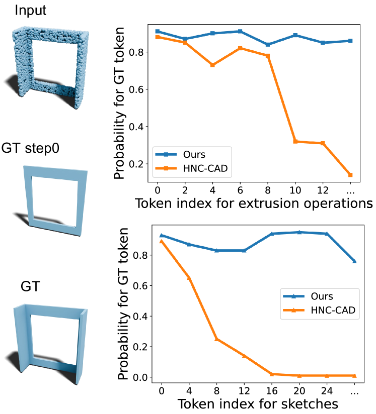
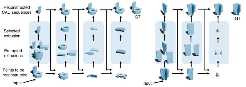
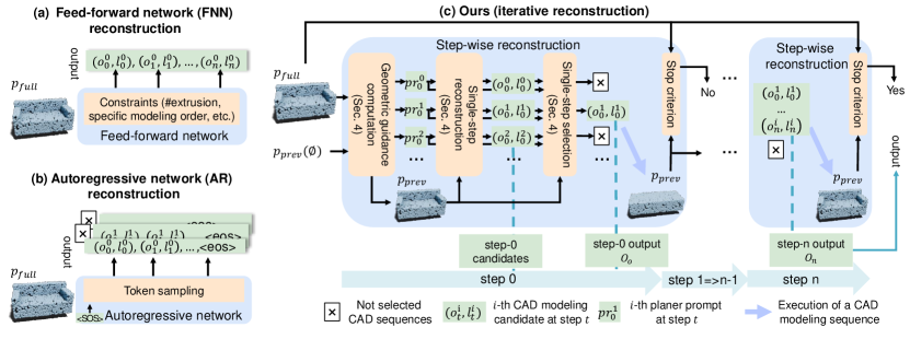
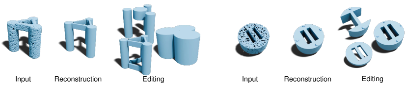
Another line of works (Wu et al., 2021; Uy et al., 2022; Ma et al., 2023; Li et al., 2023a; Lambourne et al., 2022; Khan et al., 2024) take a step further and directly learn to estimate a CAD modeling sequences from an input CAD model. These works decompose a CAD model into a list of CAD modeling steps. In our work, we adopt a domain-specific language (DSL) for CAD (Xu et al., 2022), where a CAD modeling step consists of a sketch (a 2D curve), an extrusion, and a Boolean operation (union or subtraction). The 3D shape defined by a 2D sketch and extrusion is called an extrusion cylinder. Even though previous work may have some slight deviations from this model, we use it as a common framework to structure the discussion of existing literature. There are two types of architectures used in previous work to tackle this problem. The first architecture is to generate CAD models using a feed-forward network (See Fig. 3-a, e.g. (Wu et al., 2021; Uy et al., 2022; Ma et al., 2023; Li et al., 2023a; Lambourne et al., 2022)). The feed-forward network predicts a fixed number of extrusion cylinders and Boolean operations jointly all at once, thus lacking the flexibility to adapt to input geometry with a varying number of CAD modeling steps and to sample different CAD modeling designs. The second architecture is to sequentially generate a CAD sequence using an auto-regressive deep learning model. (See Fig. 3-b, e.g. (Xu et al., 2022, 2023; Khan et al., 2024)). This model generates a CAD model one token at a time. A sequence of tokens (about 20 - 80) yields a single CAD modeling step. As each token does not have a special geometric meaning, this scheme does not consider local geometric contexts and results in a rapid descent in the softmax probability of the sampled tokens, indicating inaccurate token sampling during CAD reconstruction (See Fig. 2). We further evolve this approach to yield a third type of architecture, generating a sequence one CAD modeling step at one time (See Fig. 3-c). We call this a prompt-and-select architecture. Each iteration of our framework outputs a single CAD modeling step and consists of three components: a) geometric guidance computation, b) single-step reconstruction, and c) single-step selection. We visualize the two previous network architectures and our proposed framework in Fig. 3. Step-wise CAD reconstruction is shown in Fig. 1.
This enables us to improve upon existing auto-regressive models by providing local geometric guidance. An auto-regressive model obtains the current state as a sequence of already-generated tokens. This sequence of tokens has no immediate geometric interpretation and this requires a lot of processing to obtain a geometric interpretation before the model can reason about which token to output next. We propose to provide three types of local geometric guidance for the auto-regressive model to improve its functionality. First, we provide the difference between the current reconstruction and the input model as point cloud. This let’s the model know which parts it should focus on. Second, we geometrically analyze the model to find candidate planes from which a new CAD modeling step can be started. We then provide these candidate planes as input in the form of prompts, analog to segmentation prompts popular in recent work (Kirillov et al., 2023). This provides the context for generating the next candidate CAD modeling step and the generated sketches (curves) are encouraged to lie on the prompt planes. Third, we implement a geometric form of lookahead sampling. Instead of simply sampling one token at a time based on the computed probability, we generate multiple complete candidate CAD modeling steps (each encoded as a sequence of tokens) and then evaluate the candidates to choose the most suitable one. The network trained for this component is supervised with geometric criteria. Fig. 1 shows how the proposed modeling pipeline builds a CAD model step by step. Fig. 3-c shows the proposed network architecture.
Our main contributions are:
-
•
We propose an iterative prompt-and-select architecture to progressively reconstruct the CAD modeling sequence of a target shape.
-
•
We propose the concept of local geometric guidance for auto-regressive models and propose three ways to integrate this guidance into the auto-regressive framework.
-
•
Quantitative experiments demonstrate a significant improvement over the current state of the art. For example, on the dataset DeepCAD, our framework PS-CAD improves upon the best published SOTA method by reducing the geometry errors (CD and HD) by , and the structural error (ECD) by about .
2. Related Work
In this section, we review related works on 3D CAD reconstruction with different output formats, ranging from parametric primitives, and CSG trees, to the CAD modeling sequence.
CAD Primitive Reconstruction. Most approaches in the scheme represent an input 3D shape as a set of parametric primitives to be assembled, where the parametric primitives can be edges, surface patches, 3D solids, etc. Traditional approaches first segment and fit an input shape with basic parametric primitives (e.g. planes, spheres, and cylinders) (Schnabel et al., 2007; Kim et al., 2013; Fish et al., 2014). Recent advances in learning-based methods have improved the robustness of primitive fitting approaches (Tulsiani et al., 2017; Li et al., 2019; Yan et al., 2021) by being tolerable to outliers, meanwhile allowing for a wider variety of primitives for enhanced shape representation and better performance, including e.g. super quadratics (Paschalidou et al., 2019), convexes (Deng et al., 2020), learnable Bézier (Fu et al., 2023) and B-spline patches (Sharma et al., 2020), implicit fields (Park et al., 2019), etc. Another category of approaches (Wang et al., 2020; Guo et al., 2022b; Li et al., 2023b; Zhu et al., 2023) emphasize the preservation of sharp geometric features and learn to fit edges, corners that have a parity relation with surface patches from the input. Though these works can produce high-quality geometry, their results are mainly primitives missing the high-level CAD modeling operations, and therefore not easy to apply further editing.
CSG-tree based CAD Reconstruction. Pioneering works (Shapiro and Vossler, 1991, 1993; Buchele and Crawford, 2004; Hamza and Saitou, 2004; Fayolle and Pasko, 2016) investigate to express input 3D shape as Constructive Solid Geometry (CSG) (Laidlaw et al., 1986) with Boolean operations, well maintaining the shape construction information without loss of expressiveness. Typically, search-based algorithms and pruning strategies are applied to build CSG trees (Du et al., 2018; Wu et al., 2018). For learning-based CSG reconstruction, the key challenge is to combine the indifferentiable CSG tree construction with differentiable primitive fitting. Previous works address this problem by using reinforcement learning (Sharma et al., 2018, 2022; Ellis et al., 2019; Jones et al., 2022), recursive constructions based on hand-crafted geometric rules (Guo et al., 2022a), and novel learnable Boolean layers (Kania et al., 2020). Successive approaches specify the CSG trees with fixed order and depth (Ren et al., 2021, 2022), together with dedicated differentiable objectives and networks (Yu et al., 2022, 2023). However, to replicate the overall structure and retain fine geometric details with a fixed set of primitives, the structures of composed intermediate parts are seldom considered and therefore less interpretable and editable.
CAD Modeling sequence Reconstruction. To accommodate the modern CAD design pipeline, several approaches predict a CAD modeling sequence from a 3D CAD model. DeepCAD (Wu et al., 2021) encodes CAD modeling sequences as CAD domain-specific language (DSL) sequences and trains a transformer model conditioned on input to generate or reconstruct CAD DSL sequences directly. ZoneGraph (Xu et al., 2021) employs a zone graph to represent the CAD model given as B-rep. A zone corresponds to a 3D entity derived from the B-rep faces. In this way, predicting the CAD modeling sequence turns into a combinatorial problem in the discrete space permitted by the zone graph. Leveraging well-annotated datasets (Willis et al., 2021; Wu et al., 2021), Point2Cyl (Uy et al., 2022) derives a set of parametric extrusion cylinders with a specified set size, based on segmentation of input shape. Lambourne et al. (2022) train a network to predict sketches and extruded values with a predefined CAD modeling sequence template. SECAD-Net (Li et al., 2023a) reconstructs parametric extrusions and combines them as the input CAD model using Union operation. The closest work to ours is the concurrent CAD-SIGNet (Khan et al., 2024). It reconstructs the CAD modeling sequence using an autoregressive network. As the core design, it uses predicted extrusion operation to assist in predicting the sketch. Our approach has the following differences from CAD-SIGNet: (1) We iteratively reconstruct the CAD modeling steps that splice to the complete CAD modeling sequence, rather than output the complete CAD modeling sequence (see Fig. 3 (b) and (c) for comparison); (2) In each step we reconstruct multiple candidate CAD modeling steps based on prompts rather than token sampling (3) We devise a single-step selection module to select the best-fitted candidate, rather than rely on geometric criteria for CAD modeling sequence selection.
3. Overview
In this section, we first introduce the domain-specific language (DSL) used for encoding CAD modeling sequences in this paper. Then we give an overview of our approach. Our approach takes a 3D CAD model given as point cloud as input and outputs a DSL sequence.
3.1. Preliminaries on the CAD DSL
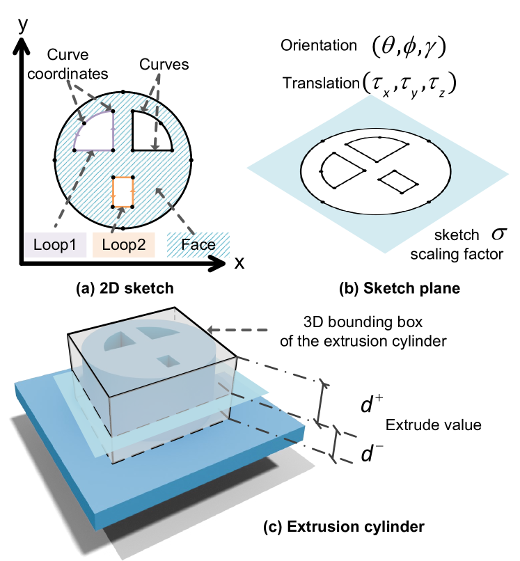
We use the CAD DSL from SkexGen (Xu et al., 2022). It decomposes a 3D CAD model into a sequence of CAD modeling steps , where is an extrusion cylinder and is a Boolean operation (union or subtraction). An extrusion cylinder consists of a 2D sketch and an extrusion operation . The CAD modeling sequence is a sequence of CAD modeling steps:
| (1) |
where is the number of CAD modeling steps. We use to define the construction of the CAD model up until step , i.e., the current state achieved by executing all with . Next, we explain how is described by a 2D sketch and extrusion . The sketch is organized as a ”sketch-face-loop-curve” hierarchy. A sketch can contain one or more faces, where a face is a 2D region bounded by one or multiple loops. A loop is a closed 2D path consisting of one or more curves. A curve is either a line segment, an arc, or a circle. See Fig. 4 for an example. A sketch is represented as a nested sequence:
| (2) |
where , , , denote the tokens to mark the end of a curve, loop, face, and sketch, respectively. is a list of four 2D coordinates to represent the outer circle in Fig. 4. To distinguish between the three types of curves, a line segment is described by 2 points, an arc by 3, and a circle by 4. The extrusion operation transforms the sketch into an extrusion cylinder :
| (3) |
Specifically, the 2D sketch is scaled with a factor of and then transformed to the sketch plane with orientation and translation . represents the extruded distances along (or opposite) the sketch plane normal. An illustration is shown in Fig. 4. Each extrusion cylinder is combined with the previous state using Boolean operation , where is for the Union or for Subtraction. In our implementation, we adopt the discrete tokenization in SkexGen (Xu et al., 2022) as the CAD DSLs to facilitate further autoregressive model learning. Additional details on the DSL tokenization and CAD modeling sequences can be found in Supp. A.
3.2. Pipeline Overview
Given an input 3D CAD model as point cloud consisting of points, we learn to reconstruct an output CAD modeling sequence encoded by the CAD DSL. To tackle the problem, we present an iterative prompt-and-select pipeline as illustrated in Fig. 3. For each iteration , the method executes the following algorithmic steps.
Geometric Guidance Computation: We can analyze the previous state defined by CAD modeling sequence and point cloud to compute two forms of geometric guidance. First, we make use of the fact that extrusion cylinders have a planar bottom and top surface. We detect a set of candidate planes that are possible starting points for the next CAD modeling step . These planes are encoded as planar prompts . Further, we compute a point cloud that encodes the difference between and the previous state as additional geometric guidance. We encode by sampling it as point cloud .
Single-Step Reconstruction: The single-step reconstruction module at step takes as inputs the planar prompts , the target point cloud and the point cloud describing the previous state . We compute a possible CAD modeling step for each sampled prompt (see the illustration in Fig. 5).
Single-Step Selection: The single-step selection module at step takes all candidate CAD modeling steps as input. We evaluate the fitness of each CAD modeling step and select the one with the highest fitness. For example, the CAD modeling step is chosen in the step-0 of Fig. 3(c). Then, we concatenate the chosen CAD modeling step to the previous state and continue with the next iteration.
The method iteratively executes the above three modules until a stop criterion is achieved, e.g., the reconstruction error is small enough. The final output is denoted as .
3.3. Common Modules
Point cloud encoder. We require a building block that can take an arbitrary point cloud and convert it into a set of tokens (features). We use the popular framework Point-MAE (Pang et al., 2022) to obtain point cloud features. We pre-train Point-MAE based on a point cloud reconstruction task following the official repo111https://github.com/Pang-Yatian/Point-MAE with input point cloud on the training dataset. Note that this pre-training is independent of the DSL sequence reconstruction. Once Point-MAE is trained, we only keep the Point-MAE encoder for point cloud features extraction. During training, we froze the first three layers and finetuned the last three layers so that the network could be adapted for our specific tasks. The point cloud encoder can encode an input point cloud to a set of tokens (features) . For example, in later sections, we use , and to denote the features computed for , and , respectively.
4. Geometric Guidance Computation
The geometric guidance computation module at iteration (time step) takes the point cloud of the complete input CAD model as input. As additional input, we execute the token sequence describing the previous state and sample the resulting CAD model with point cloud . As output we compute a set of candidate prompts .
Point Cloud Segmentation First, we would like to identify the distinct regions between and . The distinct region of compared to represents the geometry not yet covered by , while the distinct region of compared to contains auxiliary points in the construction that will no longer be present in the final model. For example, given an observation in Fig. 6(b), represents a sofa model, and represents its base. The distinct region of corresponds to the armrest of the sofa. However, point clouds for the bottom face of the armrest are absent in since it is sampled from the surface of the sofa, and the missing point cloud is complemented by the distinct region of . We train a segmentation network to predict binary masks on and , labeling points with if they belong to a distinct region. The segmentation mask is then applied to and to get distinct point cloud regions . We use the notation and to denote an operation that returns the points with label from the point cloud and , respectively. The point cloud is simply the concatenation of and .
Plane Detection We detect a set of candidate planes with an off-the-shelf RANSAC method and encode them as planar prompt . A planar prompt is encoded by randomly sampling 64 inlier points from a plane detected by RANSAC.
5. Single-step Reconstruction
This section presents a module that takes the point cloud and a single prompt as input and outputs a candidate CAD modeling step as depicted in Fig. 6(a). This module is executed for each prompt separately, but the point cloud is shared between all separate executions of the module.
We first discuss the network architecture. We use three decoders (Fig. 6) to predict three components of a CAD modeling step: sketch decoder (-dec) for , extrude decoder (-dec) for , and Boolean operation decoder (-dec) for . In addition, we use a simple module for prompt embedding. See Fig. 6 for an illustration of the architecture. We describe the individual components next.
Prompt embedding. Prompt embedding is computed by embedding the prompt point cloud using the point embedding part of the point cloud encoder. This embedding creates one token (feature vector) per point. We denote the output of this embedding as .
Sketch decoder and extrude decoder. Both sketch decoder -dec and extrude decoder -dec adopt the same transformer architecture for autoregressive sequence prediction, implemented as stacked transformer decoder blocks shown in Fig. 6(c). Therefore, we describe them together. The input at each iteration of -dec and -dec are point cloud , prompt , and the current sequence of tokens ( or ). Since both modules work in an auto-regressive manner, the modules themselves operate iteratively building the output sequences ( or ) one step at a time. We use to denote the iteration. We use as shorthand to denote the sequence . In the first iteration, or are initialized with the start token . First, all inputs are encoded: is encoded with the point cloud encoder to yield , is encoded to yield and () is encoded to yield the sequence embedding of the sketch(extrude).
The Queries of the self-attention and cross-attention layers in -dec (-dec) ) are the concatenation of and the sequence embedding of (). The same tokens also serve as keys and values for the self-attention layers. For the multi-head cross-attention layers, point cloud features , serve as Keys and Values.
To output the next token, each token is assigned a softmax probability. An operator is followed to get the token value as follows:
| (4) |
is the component index of the output probability, with a range of in and in . Q is the number of different discrete tokens for a sketch or an extrusion operation as defined in SkexGen. We then execute the predicted for a shape, from which we extract point clouds and compute features .
Boolean operation decoder. We implement -dec as a transformer following a ”Max-pooling + Linear + Sigmoid” layer, as depicted in Fig. 6(d). The -dec takes and as input, predicting a scalar in the range of to represent .
Training objective. We train -dec and -dec using teacher forcing (Kolen and Kremer, 2001) and cross-entropy loss , and train -dec with binary cross-entropy loss . However, such an objective does not lead to a good performance. Experiments show the derived shape of the output sequence largely differs from the supervision-executed shape in geometric structure and appearance. We believe this is caused by the huge domain gap between sequential and geometric representation (Ma et al., 2023), and we propose a geometric objective term to map the sequential output to the geometric representation space. Following Eq. 5, we construct a 3D bounding box of the executed shape of , and calculate its intersection-over-union (IoU) with the bounding box of the supervision-executed shape,
| (5) |
where is the supervision of , indicating the ground-truth extrusion cylinder for the step . The bbox() is a differentiable operator to construct a 3D bounding box from or . The bounding box of an executed shape of a sketch-extrude sequence is illustrated in Fig. 4(c). The overall objective function is Eq. 6, where is only enforced after training epochs.
| (6) |
6. Single-step Selection
The single-step reconstruction module generates multiple candidate CAD modeling steps . Here, we propose an architecture component that assigns probabilities to the different candidates. Though each choice consists of a sequence of tokens with corresponding probabilities (cf. Eq. 4), the probabilities are conditioned on a specific prompt. Therefore, we cannot directly compute the overall probability of each candidate CAD modeling step.
To rate different CAD modeling steps, we present a single-step selection module for addressing this task. The module is trained to measure the geometric fitness of candidate CAD modeling steps. which therefore avoids the confusion due to pertaining to the GT step, while being more efficient than brute-force enumeration that executes all candidate commands and compares them in retrospect. We use the same mathematical notations as Sec. 5 for convenience and readability.
Network architecture. A visualization of the network architecture is shown in Fig. 7. The single-step selection module (denoted as -dec) takes the point cloud , a single prompt , and a candidate CAD modeling step as input and outputs a value representing the fitness of . The -dec is implemented in the same architecture as the sketch/extrude decoder in Fig. 6(c), except the output layer is modified from the ”Linear + softmax + arg max” to the ”Linear + sigmoid”. For the input, the point cloud , the prompt , and are encoded to yield , and the sequence embedding. The Query of -dec () is the concatenation of and the sequence embedding of . serves as Key and Value. The output is as follows:
| (7) |
Training objective. The single-step selection module essentially performs a regression task and we choose the commonly used L1 loss as the objective function for step , . denotes the supervision of the fitness score for as defined in Eq. 8. Since cannot be directly obtained from the existing dataset (Wu et al., 2021), we calculate by comparing the geometric similarity between the executed shapes of and ground-truth . The intuition is that cannot be concluded as unsuitable even if it is dissimilar to . Instead, it is more reliable to compare the similarity between their unique executions. We formulate as the bounding box intersection-over-union (IoU) between the executed shape of and , multiplied by the binary value of the and consistency, where the is the same as that in Eq. 5.
| (8) |
We use the bounding box IoU to approximate the geometric similarity for two reasons. First, calculating the bounding box IoU is more straightforward compared to calculating the fine-grained IoU between shapes. Second, the bounding box can accurately reflect the principal parameters of the sketch-extrude sequence constructing the shape (cf. Extrude value, Sketch plane orientation, etc. in Fig. 4).
7. Experiments and Analysis
In this section, we provide a quantitative and qualitative evaluation, an ablation study, and a robustness test of our method.
7.1. Experimental Setup
Datasets. We use the DeepCAD (Wu et al., 2021) dataset for training. Following the dataset split of DeepCAD, we train the networks on the DeepCAD train set and report results on the DeepCAD test set. We also report the cross-dataset generalization based on the Fusion360 (Willis et al., 2021) dataset. For all input CAD models, we randomly sample 8192 points on the surface as input point clouds.
Evaluation metrics. We evaluate the geometric quality following (Guo et al., 2022a) and sequence fidelity using NLL used to evaluate similar auto-regressive generative models. Geometric metrics are calculated between the input CAD models and the execution of predicted CAD modeling sequence with the following terms:
-
•
Chamfer distance (CD) and Hausdorff distance (HD) of 16382 randomly sampled points on the geometry surface of two shapes for geometry distance.
-
•
Edge chamfer distance (ECD) to compute the distance between edge points of two CAD models to reflect the structure similarity.
-
•
Normal consistency (NC) to measure the cosine similarity between corresponding normals as the smoothness of predicted shapes.
-
•
Invalidity Ratio (IR) to measure the ratio of CAD modeling sequences that cannot be executed.
We use the point cloud of the ground-truth CAD model and the point cloud of output CAD modeling sequence execution to compute geometric metrics. For a scale-invariance comparison, we normalize the ground-truth CAD model and reconstruction into a unit bounding box keeping the aspect ratio. To determine whether a reconstruction is invalid, we retain the output of each step (). If none of them leads to a successful execution, we consider it to be invalid. We use the Negative log-likelihood (NLL) of the auto-regressive model to evaluate the sequence fidelity produced by the single-step reconstruction module. Specifically, given the point cloud of the input CAD model and that of the ground-truth previous state, we predict the logits of the next CAD modeling step and calculate the NLL. We evaluate the quality of sketch and extruding, separately with ske_NLL and ext_NLL.
Baselines. We compare with four SoTA methods (Wu et al., 2021; Xu et al., 2023; Uy et al., 2022; Li et al., 2023a; Xu et al., 2021) focusing on the reverse engineering of CAD modeling sequences. We compare with these methods by running the available codes and pre-trained weights with the same test splits for a fair comparison. Point2Cyl (Uy et al., 2022) applies instance segmentation on point cloud of the input CAD model. Each instance is treated as a potential extrusion cylinder and another segmentation is applied to locate the cross-section (base) and side surface (barrel). Afterward, Point2Cyl fit for an extrusion operation and a sketch utilizing base and barrel. SECAD-Net (Li et al., 2023a) requires both voxel and point cloud as inputs, We apply mesh-voxelization (Stutz and Geiger, 2018; Stutz, 2017) to convert the mesh of a CAD model into a voxel. It outputs a fixed number of CAD modeling steps and we follow its official implementation to output 4 CAD modeling steps. Since SECAD-Net employs unsupervised learning, it can overfit to each test data to get the best reconstruction result. HNC-CAD is initially designed for CAD modeling sequence generation. We train HNC-CAD by feeding it with the point cloud features of the input CAD model, without changing any output to adapt it to perform CAD modeling sequence reconstruction. We do not compare with (Lambourne et al., 2022) and the concurrent work (Khan et al., 2024), because they do not release the source code.
Implementation details. For geometric guidance computation (Sec. 4), we train the point cloud segmentation network for 80 epochs with a batch size of 256. An AdamW optimizer with an initial learning rate of 1e-3 is employed for optimization and the learning rate is scheduled by a cosine annealing scheduler until the minimal learning rate of 1e-6. We train the single-step reconstruction (Sec. 5) based on the objective function of Eq. 6. The network is trained for 200 epochs with a batch size of 224 on 1 A100-80G GPU, using the AdamW optimizer with a learning rate of 1e-3. The learning rate drops to 9e-5 after the initial 90 epochs and gradually decreases to the minimal learning rate of 5e-6 based on the cosine annealing scheduler. We empirically set the in Eq. 6 as 30. The single-step selection (sec. 6) is trained for 100 epochs with a batch size of 224 on 1 A100-80G GPU, using the same optimizer and learning rate scheduler as the single-step reconstruction.
7.2. Comparison with the State of the Art
| Dataset | Method | CD | HD | ECD | NC | IR () |
| DeepCAD | 4.25 | 39.25 | 19.33 | 0.49 | 7.14 | |
| HNC-CAD | 1.09 | 20.23 | 5.94 | 0.75 | 0.32 | |
| DeepCAD | Point2cyl | 1.00 | 20.93 | 20.45 | 0.73 | 0.0 |
| SECAD-Net | 0.42 | 9.96 | 5.54 | 0.73 | 0.38 | |
| Ours (PS-CAD) | 0.21 | 8.66 | 4.65 | 0.89 | 0.43 | |
| HNC-CAD | 1.38 | 20.61 | 9.24 | 0.52 | 0.33 | |
| Fusion360 | SECAD-Net | 0.69 | 12.76 | 5.15 | 0.64 | 3.82 |
| Ours (PS-CAD) | 0.57 | 12.0 | 5.02 | 0.67 | 1.51 |
| Method | ext_NLL | ske_NLL |
| HNC-CAD | 38.66 | 103.33 |
| Ours (PS-CAD) | 1.61 | 25.51 |
| Single-step reconstruction | Single-step selection | Metrics | ||||||||||
| geo | heur | rand | ours | CD | ext_NLL | ske_NLL | IR () | |||||
| 1.21 | 5.77 | 132.85 | 7.53 | |||||||||
| 0.67 | 2.24 | 91.03 | 6.85 | |||||||||
| 0.37 | 1.68 | 33.45 | 6.99 | |||||||||
| 0.61 | 1.98 | 47.84 | 1.37 | |||||||||
| 0.28 | 1.59 | 30.10 | 0.69 | |||||||||
| 0.95 | 2.49 | 100.08 | 1.37 | |||||||||
| 1.48 | 7.95 | 213.27 | 1.51 | |||||||||
| 0.19 | 1.49 | 19.63 | 0.41 | |||||||||
Main comparison. In Tab. 1, we quantitatively show the performance of all the competing methods. Directly predicting a CAD modeling sequence as the CAD DSL sequence, e.g., DeepCAD (Wu et al., 2021) and HNC-CAD (Xu et al., 2023) for this task results in poor performance because aligning point clouds with a CAD DSL is difficult. Our proposed method PS-CAD significantly improves upon all SOTA methods on all geometric metrics on DeepCAD. We can reduce the geometry errors (CD and HD) by at least , and the structural error (ECD metric) by about . Moreover, the proposed method can attain the best normal quality. The generalization comparison on Fusion360 yields better results than HNC-CAD and SECAD-Net. We reduce the geometry errors by at least and the structural error by about .
We show a comparison of the NLL in Tab. 2. We can only compare to the similar auto-regressive model HNC-CAD and we note a huge improvement in the metrics. This suggests that geometric guidance can greatly improve the accuracy of predicting CAD DSL sequences.
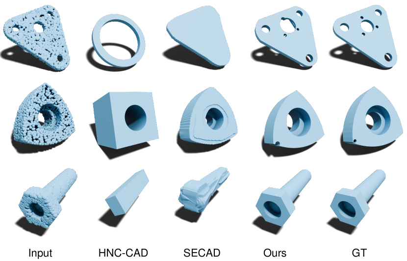
Qualitative comparison. In Fig. 8 and Fig 9, we qualitatively show the performance on DeepCAD and Fusion360 of the competing methods. Note that our point cloud visualization shows the overall structure well, but seeing some of the detailed structures in the input point cloud would require inspecting the point cloud in an interactive editor from multiple views (See Appendix Fig. 17). DeepCAD and HNC-CAD output a CAD DSL sequence. They can correctly reconstruct the coarse appearance of the input CAD models, but the structure as well as the details are often wrong. (see column DeepCAD, HNC-CAD in Fig. 8, column HNC-CAD in Fig. 9).
Point2Cyl and SECAD-Net reconstruct sketches with implicit representations and generally perform better than DeepCAD and HNC-CAD. Still, Point2Cyl and SECAD-Net also have problems with the details as well as the structure. Point2Cyl often predicts the main shape correctly, but it adds incorrect and overly complicated details (all rows in Fig. 8). SECAD-Net sometimes does not preserve the basic structures, e.g. crevices in the input (see row 2,3,6 in Fig. 8 and rows in Fig. 9) or invents erroneous details, e.g., a square extrusion cylinder in row 1 in Fig. 8. By contrast, our method reproduces the structure and the details of the input better. Our method is also capable of reconstructing detailed geometry of inputs from a cross-domain dataset Fusion360, e.g., different kinds of holes in Fig. 9.
7.3. Ablation Studies

In Tab. 3, we first show a set of ablations on the designs of the single-step reconstruction. We randomly select 730 input models for the ablation studies, which accounts for approximately 10% of the total test dataset. Note that we evaluate the designs of the single-step reconstruction with the selection strategy ”geo”. This is because the single-step selection is based on the output of the single-step reconstruction. When the output quality varies due to the ablation setting, the rating result of the single-step selection introduces extraneous factors that affect the ablation.
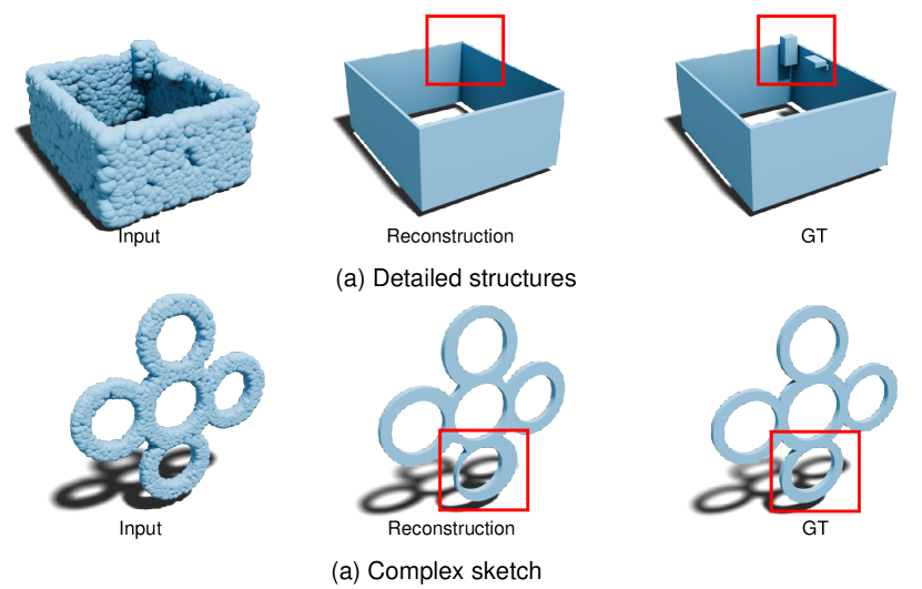
The effect of . The first three rows of Tab. 3 ablate the input fed to single-step reconstruction. Only given leads to poor performance in geometric quality and sequence fidelity. It can only reconstruct the main structure and loses many details. Sometimes an invalid reconstruction is produced (see Fig. 10 ). With the help of , there is a noticeable reduction in the extrude NLL (ext_NLL). By explicitly identifying the distinct regions of and with a binary mask , the network can distinguish which part has already been completed for reconstruction, and which part still needs further work. Using the mask gives a cleaner geometric context and improves the sequence fidelity, reflected in further reductions in sketch NLL and extrude NLL.
The effect of . By providing a prompt to the single-step reconstruction, albeit with a decrease in geometric reconstruction quality, it improves the reconstruction invalid rate. This suggests that the prompt improves the tolerance to input CAD models with different shapes. We believe the source of this ability is that the prompt can provide guidance for local geometric context encoding. This local geometric context, compared with , can support the reconstruction of one valid CAD modeling step with better efficiency.
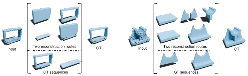
Single-step selection. Afterward, we fix the setting of single-step reconstruction and validate the single-step selection by comparing it with different selection strategies. Among the other selection strategies, ”geo” is based on the geometric quality of the candidate CAD modeling step. Take the step- for example, we make temporary step- by combining the candidate CAD modeling step with the state- output . The execution of as point cloud is compared with point cloud of the input CAD model to calculate the chamfer distance. ”geo” selects the with the lowest chamfer distance as the step- output. ”heur” is to select the extrusion cylinder with the largest volume. It follows a design convention that a CAD model is usually created by first constructing the main structure and then designing the details. ”rand” is to randomly select a candidate CAD modeling step. The results show that the heuristic and geometric-based selection do not work as well for all inputs because they do not consider the structure of the input CAD model. For example in Fig. 11 row 3, the input is a combination of two extrusion cylinders. However, the side surface is sampled as a prompt and leads to a candidate CAD modeling step with a ”T” shaped extrusion cylinder. This ”T-shape” extrusion cylinder has the lowest chamfer distance with the input and has the largest volume among all the candidates. In Fig. 11 row 1, the heuristic-based selection works well, but the geometric-based selection performs badly and creates two boxes using the green prompt. The reason is that the chamfer distance of the CAD modeling step stemming from the green prompt is slightly better. The geometric-based selection then chooses the wrong candidate. By contrast, the single-step selection performs well in both cases, while it may select a different candidate from the ground-truth, the selected candidate can still correctly reflect the input structure.
7.4. Robustness test
In this section, we test the robustness of the single-step reconstruction module with respect to the prompt. We specifically test the effect of prompt sampling under different conditions, including the number of points of a sampled prompt, the source (sampled from either or ), and the quality of the prompt-sampling plane. Finally, we visualize some reconstruction results when our method is fed with noisy point clouds of the input CAD model.
Prompt. In Tab. 4-Sampling location, we detect planes from point clouds of different sources ( or ) and sample prompts from these planes. Results show that if the planes are sampled from the point cloud of the input CAD model in step-wise reconstruction, the performance decreases in all metrics. The extrude and sketch NLL deteriorate more than (0.190.48) and (1.493.18). If a prompt is always from , it lacks the ability to adapt to the dynamically changing geometric context in the iterative reconstruction.
In Tab. 4-Sampling number, we verify the effect of the number of points within a prompt. Given planes detected from the point cloud , the prompts with fewer points lead to a higher reconstruction invalid ratio (prompt points 6416, IR 0.410.83).
Since the prompt relies on RANSAC-detected planes, they do not always match the surface of extrusion cylinders to a high degree. In Tab. 5-Perturbations on planes, we sample prompts from planes with different corruptions, including plane deficiency or (and) Gaussian noise. Results show that our method is robust to the Gaussian noise added on prompts. When a prompt is sampled from a plane with deficiency, it cannot capture the sketch information and produces weaker reconstructions (ske_NLL from 19.51 to 33.99). This also leads to a higher invalid reconstruction ratio (IR) and chamfer distance (CD).
It is also critical to validate the effect of the RANSAC hyperparameters on prompt sampling. We test two of the hyperparameters in Tab. 5-Hyperparameters of RANSAC, namely t and d. t is the threshold value to determine when a point is detected to fit a plane. If t increases, the detected plane deviates from the real sketch plane and produces worse sketches (ske_NLL from 19.51 to 81.64, when t from 1e-3 to 1e-2). Due to the association of extrusion and the sketch plane, the extrude quality also decreases (ext_NLL 1.49 1.95). These factors result in higher IR and CD. d is the number of inlier points required to assert that a plane is fitted. If d is provided with a larger number (64 128 256), some sketches located on a tinner plane would be omitted and this results in a higher IR (0.27 0.41 2.30).
| Sampling location | Sampling number | Metrics | ||||||
| 16 | 32 | 64 | CD | ext_NLL | ske_NLL | IR | ||
| 0.48 | 3.18 | 107.04 | 1.78 | |||||
| 0.19 | 1.49 | 19.63 | 0.41 | |||||
| 0.19 | 1.53 | 20.46 | 0.83 | |||||
| 0.20 | 1.51 | 20.53 | 0.54 | |||||
| Perturbations on planes | Hyperparameters of RANSAC | Metrics | |||||
| Gaussian | deficiency 50% | t | d | CD | ext_NLL | ske_NLL | IR |
| 1e-3 | 128 | 0.19 | 1.49 | 19.51 | 0.41 | ||
| 1e-3 | 128 | 0.19 | 1.53 | 20.33 | 0.54 | ||
| 1e-3 | 128 | 0.34 | 1.69 | 33.99 | 1.65 | ||
| 1e-3 | 128 | 0.35 | 1.70 | 34.10 | 1.78 | ||
| 1e-3 | 64 | 0.23 | 1.62 | 18.65 | 0.27 | ||
| 1e-3 | 256 | 0.23 | 1.65 | 21.14 | 2.30 | ||
| 3e-3 | 128 | 0.25 | 1.60 | 20.62 | 0.27 | ||
| 5e-3 | 128 | 0.37 | 1.83 | 46.70 | 2.33 | ||
| 1e-2 | 128 | 0.39 | 1.95 | 81.63 | 1.92 | ||
| Point cloud config | layer | CD | ECD | IR |
| 6 | 0.17 | 3.80 | 0.97 | |
| 6 | 0.19 | 3.87 | 0.41 | |
| 6 | 0.17 | 3.89 | 0.28 | |
| 12 | 0.16 | 3.53 | 0.28 |
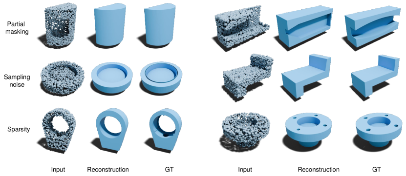
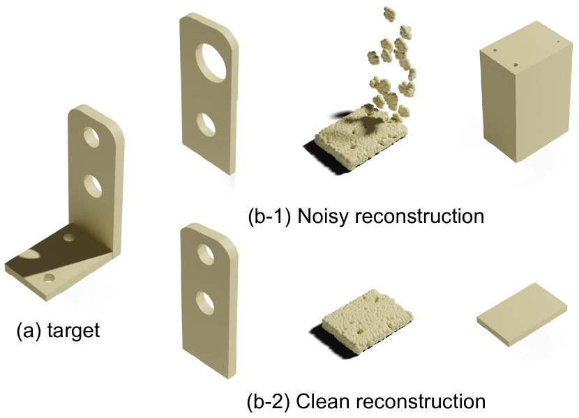
Point cloud corruptions and point cloud encoder. We validate the robustness of the method to different point cloud corruptions, like noises, sparsity, and partial point masking, in Fig. 12. We observe that the basic structure of a shape can be reconstructed, however, the local details are not consistent with the input CAD model due to noise or incomplete point clouds. We test the robustness of the method to different numbers of points in the input point clouds in Tab. 6. Results indicate sparse point clouds lead to worse results on geometric metrics. This is because point clouds with fewer points are not able to represent small-scale geometry making the CAD reconstruction with fine-level details difficult.
We also show the impact of different numbers of Transformer layers in the point cloud encoder. More Transformer layers can increase the representation capacity of the network, thus improving the metrics.
7.5. Discussions
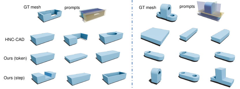
Prompt sampling vs. Token sampling. In Fig. 13, we show the capability of prompt sampling over the token sampling of the autoregressive model. In HNC-CAD, the sampling results lead to diverse CAD modeling steps, but few of them convey the structure of the input model. In Ours (token), we turn to use token sampling to produce candidate CAD modeling steps and the results are almost the same. With the help or prompt shown in different colors, Ours (step) can produce multiple reasonable candidates.
Relationship with cross-section-based methods. In geometric guidance computation, we sample planar prompts on RANSAC-detected planes. These planes are potential cross-sections which an extrusion cylinder can start from. As shown in Fig. 13, by utilizing prompts, our approach can reconstruct the extrusion cylinder highly correlated with the cross-section. From this perspective, our approach is similar to the cross-section-based method Point2Cyl. Different from Point2Cyl which uses a closed-form formulation to calculate extrusion parameters, we use the network to predict the extrusion operation. The network is more robust to the input and produces powerful geometric descriptors for reconstruction.
Failure cases. In Fig. 16, we demonstrate two typical failure cases. In the first case, the input shape contains an extrusion with a larger size and two small blocks. The method fails to recover the two small blocks as they contain very few points. In the second case, the input shape is extruded from a complex sketch and the method predicts an invalid sketch that is too different from the input.
7.6. Applications
Interactive reconstruction. Our method can produce different reconstruction sequences for the same input. This advantage can be attributed to the promptable reconstruction, which facilitates multiple legitimate candidate reconstructions in each stage. In addition to always selecting the best candidate in the single-step selection, it is also possible to sample according to probabilities. Illustrations are shown in Fig. 14. This sampling can still lead to correct reconstructions.
Moreover, we can explore potential variations of a reconstructed CAD shape by editing parameters within the reconstructed CAD modeling sequence (e.g., see Figure. 15).
8. Conclusion and Future Work
We present a prompt-and-select framework for sequential CAD modeling from point clouds. The method leverages local geometric information to guide the CAD reconstruction process of an autoregressive model. We provide plane-based prompts for better candidate sketch-extrusion sequence prediction. Extensive experiments validate the method is effective and can outperform SoTA methods in geometry accuracy (CD, HD, and ECD metrics), valid ratios, and geometry regularity (NC). We also showcase that the method can be applied to reverse engineering and further geometry editing.
There are some limitations to our work. First, we did not consider the regularity constraints between different sketch-extrusions, e.g., co-axes, alignment, and orthogonal relations between different surfaces. Second, the method mainly focuses on the CAD modeling of sketch-extrusion-based shapes and does not deal with operations like sweeping and revolving surfaces. However, it should be possible to extend it to different kinds of CAD commands when corresponding datasets are available for training. Third, fine-grained geometry details usually pose challenges to both our method and previous work. These details are usually under-represented in input point clouds and optimization losses compared to larger geometry primitives.
References
- (1)
- Buchele and Crawford (2004) Suzanne F. Buchele and Richard H. Crawford. 2004. Three-dimensional halfspace constructive solid geometry tree construction from implicit boundary representations. Comput. Aided Des. 36, 11 (2004), 1063–1073. https://doi.org/10.1016/J.CAD.2004.01.006
- Deng et al. (2020) Boyang Deng, Kyle Genova, Soroosh Yazdani, Sofien Bouaziz, Geoffrey E. Hinton, and Andrea Tagliasacchi. 2020. CvxNet: Learnable Convex Decomposition. In 2020 IEEE/CVF Conference on Computer Vision and Pattern Recognition, CVPR 2020, Seattle, WA, USA, June 13-19, 2020. Computer Vision Foundation / IEEE, 31–41. https://doi.org/10.1109/CVPR42600.2020.00011
- Du et al. (2018) Tao Du, Jeevana Priya Inala, Yewen Pu, Andrew Spielberg, Adriana Schulz, Daniela Rus, Armando Solar-Lezama, and Wojciech Matusik. 2018. InverseCSG: automatic conversion of 3D models to CSG trees. ACM Trans. Graph. 37, 6 (2018), 213. https://doi.org/10.1145/3272127.3275006
- Ellis et al. (2019) Kevin Ellis, Maxwell I. Nye, Yewen Pu, Felix Sosa, Josh Tenenbaum, and Armando Solar-Lezama. 2019. Write, Execute, Assess: Program Synthesis with a REPL. In Advances in Neural Information Processing Systems 32: Annual Conference on Neural Information Processing Systems 2019, NeurIPS 2019, December 8-14, 2019, Vancouver, BC, Canada, Hanna M. Wallach, Hugo Larochelle, Alina Beygelzimer, Florence d’Alché-Buc, Emily B. Fox, and Roman Garnett (Eds.). 9165–9174. https://proceedings.neurips.cc/paper/2019/hash/50d2d2262762648589b1943078712aa6-Abstract.html
- Fayolle and Pasko (2016) Pierre-Alain Fayolle and Alexander A. Pasko. 2016. An evolutionary approach to the extraction of object construction trees from 3D point clouds. Comput. Aided Des. 74 (2016), 1–17. https://doi.org/10.1016/J.CAD.2016.01.001
- Fish et al. (2014) Noa Fish, Melinos Averkiou, Oliver van Kaick, Olga Sorkine-Hornung, Daniel Cohen-Or, and Niloy J. Mitra. 2014. Meta-representation of shape families. ACM Trans. Graph. 33, 4 (2014), 34:1–34:11. https://doi.org/10.1145/2601097.2601185
- Fu et al. (2023) Rao Fu, Cheng Wen, Qian Li, Xiao Xiao, and Pierre Alliez. 2023. BPNet: Bézier Primitive Segmentation on 3D Point Clouds. In Proceedings of the Thirty-Second International Joint Conference on Artificial Intelligence, IJCAI 2023, 19th-25th August 2023, Macao, SAR, China. ijcai.org, 754–762. https://doi.org/10.24963/IJCAI.2023/84
- Guo et al. (2022b) Haoxiang Guo, Shilin Liu, Hao Pan, Yang Liu, Xin Tong, and Baining Guo. 2022b. ComplexGen: CAD reconstruction by B-rep chain complex generation. ACM Trans. Graph. 41, 4 (2022), 129:1–129:18. https://doi.org/10.1145/3528223.3530078
- Guo et al. (2022a) Hao-Xiang Guo, Yang Liu, Hao Pan, and Baining Guo. 2022a. Implicit Conversion of Manifold B-Rep Solids by Neural Halfspace Representation. ACM Trans. Graph. 41, 6 (2022), 276:1–276:15. https://doi.org/10.1145/3550454.3555502
- Hamza and Saitou (2004) Karim Hamza and Kazuhiro Saitou. 2004. Optimization of Constructive Solid Geometry Via a Tree-Based Multi-objective Genetic Algorithm. In Genetic and Evolutionary Computation - GECCO 2004, Genetic and Evolutionary Computation Conference, Seattle, WA, USA, June 26-30, 2004, Proceedings, Part II (Lecture Notes in Computer Science, Vol. 3103), Kalyanmoy Deb, Riccardo Poli, Wolfgang Banzhaf, Hans-Georg Beyer, Edmund K. Burke, Paul J. Darwen, Dipankar Dasgupta, Dario Floreano, James A. Foster, Mark Harman, Owen Holland, Pier Luca Lanzi, Lee Spector, Andrea Tettamanzi, Dirk Thierens, and Andrew M. Tyrrell (Eds.). Springer, 981–992. https://doi.org/10.1007/978-3-540-24855-2_110
- He et al. (2022) Kaiming He, Xinlei Chen, Saining Xie, Yanghao Li, Piotr Dollár, and Ross B. Girshick. 2022. Masked Autoencoders Are Scalable Vision Learners. In IEEE/CVF Conference on Computer Vision and Pattern Recognition, CVPR 2022, New Orleans, LA, USA, June 18-24, 2022. IEEE, 15979–15988. https://doi.org/10.1109/CVPR52688.2022.01553
- Jones et al. (2022) R. Kenny Jones, Homer Walke, and Daniel Ritchie. 2022. PLAD: Learning to Infer Shape Programs with Pseudo-Labels and Approximate Distributions. In IEEE/CVF Conference on Computer Vision and Pattern Recognition, CVPR 2022, New Orleans, LA, USA, June 18-24, 2022. IEEE, 9861–9870. https://doi.org/10.1109/CVPR52688.2022.00964
- Kania et al. (2020) Kacper Kania, Maciej Zieba, and Tomasz Kajdanowicz. 2020. UCSG-NET- Unsupervised Discovering of Constructive Solid Geometry Tree. In Advances in Neural Information Processing Systems 33: Annual Conference on Neural Information Processing Systems 2020, NeurIPS 2020, December 6-12, 2020, virtual, Hugo Larochelle, Marc’Aurelio Ranzato, Raia Hadsell, Maria-Florina Balcan, and Hsuan-Tien Lin (Eds.). https://proceedings.neurips.cc/paper/2020/hash/63d5fb54a858dd033fe90e6e4a74b0f0-Abstract.html
- Khan et al. (2024) Mohammad Sadil Khan, Elona Dupont, Sk Aziz Ali, Kseniya Cherenkova, Anis Kacem, and Djamila Aouada. 2024. CAD-SIGNet: CAD Language Inference from Point Clouds using Layer-wise Sketch Instance Guided Attention. arXiv:2402.17678 [cs.CV]
- Kim et al. (2013) Vladimir G. Kim, Wilmot Li, Niloy J. Mitra, Siddhartha Chaudhuri, Stephen DiVerdi, and Thomas A. Funkhouser. 2013. Learning part-based templates from large collections of 3D shapes. ACM Trans. Graph. 32, 4 (2013), 70:1–70:12. https://doi.org/10.1145/2461912.2461933
- Kirillov et al. (2023) Alexander Kirillov, Eric Mintun, Nikhila Ravi, Hanzi Mao, Chloé Rolland, Laura Gustafson, Tete Xiao, Spencer Whitehead, Alexander C. Berg, Wan-Yen Lo, Piotr Dollár, and Ross B. Girshick. 2023. Segment Anything. In IEEE/CVF International Conference on Computer Vision, ICCV 2023, Paris, France, October 1-6, 2023. IEEE, 3992–4003. https://doi.org/10.1109/ICCV51070.2023.00371
- Kolen and Kremer (2001) John F Kolen and Stefan C Kremer. 2001. A field guide to dynamical recurrent networks. John Wiley & Sons.
- Laidlaw et al. (1986) David H. Laidlaw, W. Benjamin Trumbore, and John F. Hughes. 1986. Constructive solid geometry for polyhedral objects. In Proceedings of the 13th Annual Conference on Computer Graphics and Interactive Techniques, SIGGRAPH 1986, Dallas, Texas, USA, August 18-22, 1986, David C. Evans and Russell J. Athay (Eds.). ACM, 161–170. https://doi.org/10.1145/15922.15904
- Lambourne et al. (2022) Joseph George Lambourne, Karl D. D. Willis, Pradeep Kumar Jayaraman, Longfei Zhang, Aditya Sanghi, and Kamal Rahimi Malekshan. 2022. Reconstructing editable prismatic CAD from rounded voxel models. In SIGGRAPH Asia 2022 Conference Papers, SA 2022, Daegu, Republic of Korea, December 6-9, 2022, Soon Ki Jung, Jehee Lee, and Adam W. Bargteil (Eds.). ACM, 53:1–53:9. https://doi.org/10.1145/3550469.3555424
- Li et al. (2019) Lingxiao Li, Minhyuk Sung, Anastasia Dubrovina, Li Yi, and Leonidas J. Guibas. 2019. Supervised Fitting of Geometric Primitives to 3D Point Clouds. In IEEE Conference on Computer Vision and Pattern Recognition, CVPR 2019, Long Beach, CA, USA, June 16-20, 2019. Computer Vision Foundation / IEEE, 2652–2660. https://doi.org/10.1109/CVPR.2019.00276
- Li et al. (2023a) Pu Li, Jianwei Guo, Xiaopeng Zhang, and Dong-Ming Yan. 2023a. SECAD-Net: Self-Supervised CAD Reconstruction by Learning Sketch-Extrude Operations. In IEEE/CVF Conference on Computer Vision and Pattern Recognition, CVPR 2023, Vancouver, BC, Canada, June 17-24, 2023. IEEE, 16816–16826. https://doi.org/10.1109/CVPR52729.2023.01613
- Li et al. (2023b) Yuanqi Li, Shun Liu, Xinran Yang, Jianwei Guo, Jie Guo, and Yanwen Guo. 2023b. Surface and Edge Detection for Primitive Fitting of Point Clouds. In ACM SIGGRAPH 2023 Conference Proceedings, SIGGRAPH 2023, Los Angeles, CA, USA, August 6-10, 2023, Erik Brunvand, Alla Sheffer, and Michael Wimmer (Eds.). ACM, 44:1–44:10. https://doi.org/10.1145/3588432.3591522
- Ma et al. (2023) Weijian Ma, Minyang Xu, Xueyang Li, and Xiangdong Zhou. 2023. MultiCAD: Contrastive Representation Learning for Multi-modal 3D Computer-Aided Design Models. In Proceedings of the 32nd ACM International Conference on Information and Knowledge Management. 1766–1776.
- Pang et al. (2022) Yatian Pang, Wenxiao Wang, Francis E. H. Tay, Wei Liu, Yonghong Tian, and Li Yuan. 2022. Masked Autoencoders for Point Cloud Self-supervised Learning. In Computer Vision - ECCV 2022 - 17th European Conference, Tel Aviv, Israel, October 23-27, 2022, Proceedings, Part II (Lecture Notes in Computer Science, Vol. 13662), Shai Avidan, Gabriel J. Brostow, Moustapha Cissé, Giovanni Maria Farinella, and Tal Hassner (Eds.). Springer, 604–621. https://doi.org/10.1007/978-3-031-20086-1_35
- Park et al. (2019) Jeong Joon Park, Peter R. Florence, Julian Straub, Richard A. Newcombe, and Steven Lovegrove. 2019. DeepSDF: Learning Continuous Signed Distance Functions for Shape Representation. In IEEE Conference on Computer Vision and Pattern Recognition, CVPR 2019, Long Beach, CA, USA, June 16-20, 2019. Computer Vision Foundation / IEEE, 165–174. https://doi.org/10.1109/CVPR.2019.00025
- Paschalidou et al. (2019) Despoina Paschalidou, Ali Osman Ulusoy, and Andreas Geiger. 2019. Superquadrics Revisited: Learning 3D Shape Parsing Beyond Cuboids. In IEEE Conference on Computer Vision and Pattern Recognition, CVPR 2019, Long Beach, CA, USA, June 16-20, 2019. Computer Vision Foundation / IEEE, 10344–10353. https://doi.org/10.1109/CVPR.2019.01059
- Ren et al. (2021) Daxuan Ren, Jianmin Zheng, Jianfei Cai, Jiatong Li, Haiyong Jiang, Zhongang Cai, Junzhe Zhang, Liang Pan, Mingyuan Zhang, Haiyu Zhao, and Shuai Yi. 2021. CSG-Stump: A Learning Friendly CSG-Like Representation for Interpretable Shape Parsing. In 2021 IEEE/CVF International Conference on Computer Vision, ICCV 2021, Montreal, QC, Canada, October 10-17, 2021. IEEE, 12458–12467. https://doi.org/10.1109/ICCV48922.2021.01225
- Ren et al. (2022) Daxuan Ren, Jianmin Zheng, Jianfei Cai, Jiatong Li, and Junzhe Zhang. 2022. ExtrudeNet: Unsupervised Inverse Sketch-and-Extrude for Shape Parsing. In Computer Vision - ECCV 2022 - 17th European Conference, Tel Aviv, Israel, October 23-27, 2022, Proceedings, Part II (Lecture Notes in Computer Science, Vol. 13662), Shai Avidan, Gabriel J. Brostow, Moustapha Cissé, Giovanni Maria Farinella, and Tal Hassner (Eds.). Springer, 482–498. https://doi.org/10.1007/978-3-031-20086-1_28
- Schnabel et al. (2007) Ruwen Schnabel, Roland Wahl, and Reinhard Klein. 2007. Efficient RANSAC for Point-Cloud Shape Detection. Comput. Graph. Forum 26, 2 (2007), 214–226. https://doi.org/10.1111/J.1467-8659.2007.01016.X
- Shapiro and Vossler (1991) Vadim Shapiro and Donald L. Vossler. 1991. Construction and optimization of CSG representations. Comput. Aided Des. 23, 1 (1991), 4–20. https://doi.org/10.1016/0010-4485(91)90077-A
- Shapiro and Vossler (1993) Vadim Shapiro and Donald L. Vossler. 1993. Separation for Boundary to CSG Conversion. ACM Trans. Graph. 12, 1 (1993), 35–55. https://doi.org/10.1145/169728.169723
- Sharma et al. (2018) Gopal Sharma, Rishabh Goyal, Difan Liu, Evangelos Kalogerakis, and Subhransu Maji. 2018. CSGNet: Neural Shape Parser for Constructive Solid Geometry. In 2018 IEEE Conference on Computer Vision and Pattern Recognition, CVPR 2018, Salt Lake City, UT, USA, June 18-22, 2018. Computer Vision Foundation / IEEE Computer Society, 5515–5523. https://doi.org/10.1109/CVPR.2018.00578
- Sharma et al. (2022) Gopal Sharma, Rishabh Goyal, Difan Liu, Evangelos Kalogerakis, and Subhransu Maji. 2022. Neural Shape Parsers for Constructive Solid Geometry. IEEE Trans. Pattern Anal. Mach. Intell. 44, 5 (2022), 2628–2640. https://doi.org/10.1109/TPAMI.2020.3044749
- Sharma et al. (2020) Gopal Sharma, Difan Liu, Subhransu Maji, Evangelos Kalogerakis, Siddhartha Chaudhuri, and Radomír Mech. 2020. ParSeNet: A Parametric Surface Fitting Network for 3D Point Clouds. In Computer Vision - ECCV 2020 - 16th European Conference, Glasgow, UK, August 23-28, 2020, Proceedings, Part VII (Lecture Notes in Computer Science, Vol. 12352), Andrea Vedaldi, Horst Bischof, Thomas Brox, and Jan-Michael Frahm (Eds.). Springer, 261–276. https://doi.org/10.1007/978-3-030-58571-6_16
- Stutz (2017) David Stutz. 2017. Learning Shape Completion from Bounding Boxes with CAD Shape Priors. http://davidstutz.de/.
- Stutz and Geiger (2018) David Stutz and Andreas Geiger. 2018. Learning 3D Shape Completion from Laser Scan Data with Weak Supervision. In IEEE Conference on Computer Vision and Pattern Recognition (CVPR). IEEE Computer Society.
- Tulsiani et al. (2017) Shubham Tulsiani, Hao Su, Leonidas J Guibas, Alexei A Efros, and Jitendra Malik. 2017. Learning shape abstractions by assembling volumetric primitives. In Proceedings of the IEEE Conference on Computer Vision and Pattern Recognition. 2635–2643.
- Uy et al. (2022) Mikaela Angelina Uy, Yen-Yu Chang, Minhyuk Sung, Purvi Goel, Joseph Lambourne, Tolga Birdal, and Leonidas J. Guibas. 2022. Point2Cyl: Reverse Engineering 3D Objects from Point Clouds to Extrusion Cylinders. In IEEE/CVF Conference on Computer Vision and Pattern Recognition, CVPR 2022, New Orleans, LA, USA, June 18-24, 2022. IEEE, 11840–11850. https://doi.org/10.1109/CVPR52688.2022.01155
- Wang et al. (2023) Haiping Wang, Yuan Liu, Qingyong Hu, Bing Wang, Jianguo Chen, Zhen Dong, Yulan Guo, Wenping Wang, and Bisheng Yang. 2023. Roreg: Pairwise point cloud registration with oriented descriptors and local rotations. IEEE Transactions on Pattern Analysis and Machine Intelligence (2023).
- Wang et al. (2020) Xiaogang Wang, Yuelang Xu, Kai Xu, Andrea Tagliasacchi, Bin Zhou, Ali Mahdavi-Amiri, and Hao Zhang. 2020. PIE-NET: Parametric Inference of Point Cloud Edges. In Advances in Neural Information Processing Systems 33: Annual Conference on Neural Information Processing Systems 2020, NeurIPS 2020, December 6-12, 2020, virtual, Hugo Larochelle, Marc’Aurelio Ranzato, Raia Hadsell, Maria-Florina Balcan, and Hsuan-Tien Lin (Eds.). https://proceedings.neurips.cc/paper/2020/hash/e94550c93cd70fe748e6982b3439ad3b-Abstract.html
- Willis et al. (2021) Karl D. D. Willis, Yewen Pu, Jieliang Luo, Hang Chu, Tao Du, Joseph G. Lambourne, Armando Solar-Lezama, and Wojciech Matusik. 2021. Fusion 360 gallery: a dataset and environment for programmatic CAD construction from human design sequences. ACM Trans. Graph. 40, 4 (2021), 54:1–54:24. https://doi.org/10.1145/3450626.3459818
- Wu et al. (2018) Q. Wu, K. Xu, and Jun Wang. 2018. Constructing 3D CSG Models from 3D Raw Point Clouds. Comput. Graph. Forum 37, 5 (2018), 221–232. https://doi.org/10.1111/CGF.13504
- Wu et al. (2021) Rundi Wu, Chang Xiao, and Changxi Zheng. 2021. DeepCAD: A Deep Generative Network for Computer-Aided Design Models. In 2021 IEEE/CVF International Conference on Computer Vision, ICCV 2021, Montreal, QC, Canada, October 10-17, 2021. IEEE, 6752–6762. https://doi.org/10.1109/ICCV48922.2021.00670
- Xu et al. (2023) Xiang Xu, Pradeep Kumar Jayaraman, Joseph George Lambourne, Karl D. D. Willis, and Yasutaka Furukawa. 2023. Hierarchical Neural Coding for Controllable CAD Model Generation. In International Conference on Machine Learning, ICML 2023, 23-29 July 2023, Honolulu, Hawaii, USA (Proceedings of Machine Learning Research, Vol. 202), Andreas Krause, Emma Brunskill, Kyunghyun Cho, Barbara Engelhardt, Sivan Sabato, and Jonathan Scarlett (Eds.). PMLR, 38443–38461. https://proceedings.mlr.press/v202/xu23f.html
- Xu et al. (2021) Xianghao Xu, Wenzhe Peng, Chin-Yi Cheng, Karl D. D. Willis, and Daniel Ritchie. 2021. Inferring CAD Modeling Sequences Using Zone Graphs. In IEEE Conference on Computer Vision and Pattern Recognition, CVPR 2021, virtual, June 19-25, 2021. Computer Vision Foundation / IEEE, 6062–6070. https://doi.org/10.1109/CVPR46437.2021.00600
- Xu et al. (2022) Xiang Xu, Karl DD Willis, Joseph G Lambourne, Chin-Yi Cheng, Pradeep Kumar Jayaraman, and Yasutaka Furukawa. 2022. SkexGen: Autoregressive Generation of CAD Construction Sequences with Disentangled Codebooks. In International Conference on Machine Learning. PMLR, 24698–24724.
- Yan et al. (2021) Siming Yan, Zhenpei Yang, Chongyang Ma, Haibin Huang, Etienne Vouga, and Qixing Huang. 2021. HPNet: Deep Primitive Segmentation Using Hybrid Representations. In 2021 IEEE/CVF International Conference on Computer Vision, ICCV 2021, Montreal, QC, Canada, October 10-17, 2021. IEEE, 2733–2742. https://doi.org/10.1109/ICCV48922.2021.00275
- Yu et al. (2023) Fenggen Yu, Qimin Chen, Maham Tanveer, Ali Mahdavi-Amiri, and Hao Zhang. 2023. DCSG: Unsupervised Learning of Compact CSG Trees with Dual Complements and Dropouts. In Advances in Neural Information Processing Systems 36: Annual Conference on Neural Information Processing Systems 2023, NeurIPS 2023, New Orleans, LA, USA, December 10 - 16, 2023, Alice Oh, Tristan Naumann, Amir Globerson, Kate Saenko, Moritz Hardt, and Sergey Levine (Eds.). http://papers.nips.cc/paper_files/paper/2023/hash/4732d425125832887f6c5a9675d49ead-Abstract-Conference.html
- Yu et al. (2022) Fenggen Yu, Zhiqin Chen, Manyi Li, Aditya Sanghi, Hooman Shayani, Ali Mahdavi-Amiri, and Hao Zhang. 2022. CAPRI-Net: Learning Compact CAD Shapes with Adaptive Primitive Assembly. In IEEE/CVF Conference on Computer Vision and Pattern Recognition, CVPR 2022, New Orleans, LA, USA, June 18-24, 2022. IEEE, 11758–11768. https://doi.org/10.1109/CVPR52688.2022.01147
- Zhu et al. (2023) Xiangyu Zhu, Dong Du, Weikai Chen, Zhiyou Zhao, Yinyu Nie, and Xiaoguang Han. 2023. NerVE: Neural Volumetric Edges for Parametric Curve Extraction from Point Cloud. In IEEE/CVF Conference on Computer Vision and Pattern Recognition, CVPR 2023, Vancouver, BC, Canada, June 17-24, 2023. IEEE, 13601–13610. https://doi.org/10.1109/CVPR52729.2023.01307
Appendix A CAD Domain-specific language Sequence
The domain-specific language (DSL) defined by SkexGen (Xu et al., 2022) contains the most frequently used CAD modeling operations, including curves {line, arc, circle}, feature operation {extrude}, and Boolean operation {union, subtraction}. Tab. 7 provides the overview of the tokens and parameters of the DSL in SkexGen (Xu et al., 2022). SkexGen introduces a set of special tokens to denote different types of CAD modeling operations, where marks the end of ”[operation type]”, e.g. for the end of a curve and the end of extrusion. The parameters are supposed to be continuous and we follow previous works (Wu et al., 2021; Xu et al., 2022, 2023) to quantize them into discrete values to simplify the auto-regressive learning of the CAD DSL sequence. We have Eq. 9 for the quantization,
| (9) |
where is the continuous value of a parameter, is its quantization counterpart. and are the range of , is Floor operation, is the number of quantization bins of the , i.e. to determine the number of divisions from to .
As a counterpart, we formulate the value dequantization as Eq. 10 to convert back to a continuous value,
| (10) |
where the is the dequantized approximation of . The difference between and is less than .
| Operation | Token Type | Token Value Range | Description |
| 1 | End of a Sketch | ||
| 2 | End of a Face | ||
| Sketch | 3 | End of a Loop | |
| 4 | End of a Curve | ||
| Curve | |||
| Coordinates | |||
| Extruded Distance Towards Sketch Plane Normal | |||
| Extruded Distance Opposite Sketch Plane Normal | |||
| Extrude | Sketch Plane Origin | ||
| Sketch Plane Orientation | |||
| Sketch Scaling Factor | |||
| 1 | End of an Extruding Parameters | ||
| Boolean Operations | {Union, Subtraction} |
|---|
The sketch part is organized as a hierarchy of multiple curves that make up the normalized sketch. Specifically, represents a ”sketch-face-loop” hierarchy, in which a sketch can contain one or more faces, with a face being a 2D region bounded by loops. The loop is a closed path consisting of one or more curves. We use to represent the separation of hierarchical elements in . Different types of curves are uniformly noted as , identified by different numbers of curve parameters:
-
•
Line–2 operation parameters, Start and End point.
-
•
Arc–3 operation parameters, Start, Mid, and End point.
-
•
Circle–4 operation parameters, 4 points that connect into mutual orthogonal diameters.
The curve parameters are 2D coordinates on the XY-axis and will be projected onto the sketch plane through the linear transformation derived from the extrude operation. In particular, given an arbitrary point on a curve , the Euler angle , the translation vector , and the scaling factor , the projected point is given by Eq. 11,
| (11) |
where combines the Euler angles in a rotation matrix in the orthogonal group .
Appendix B Point Cloud Encoder
We implement the Point-MAE (He et al., 2022) encoder to extract point cloud features. Specifically, the input point cloud is first divided into irregular point patches via Farthest Point Sampling (FPS) and K-Nearest Neighborhood (KNN) retrieval. Formally, we have:
| (12) |
where is the input point cloud, FPS samples points as centers of point patches, and KNN selects nearest points from for each point patch. The embedding of the point patch is calculated as:
| (13) |
where PointNet is a lightweight MLP+max-pooling layer, and PE is a learnable positional embedding also implemented as an MLP layer. is the number of feature channels. is then fed into a standard transformer. Each transformer block is implemented as a multi-head self-attention (SA) + MLP layer. The positional embedding is added to each block to provide point position information. The output of the transformer is the features of point cloud , denoted as . To balance cost and performance, we set in KNN, . The number of transformer blocks is set as 6.
Appendix C Point Cloud Segmentation Network
We train a segmentation network to compare the differing regions between and . The point cloud segmentation network consists of the Point-MAE encoder, a decoder, and a mask prediction head. The Decoder adopts three Transformer blocks and takes the concatenation of point cloud features as input and outputs the features which is fed to the mask prediction head. The mask prediction head is implemented as a fully connected layer to project to a point cloud mask . Then followed by a reshape and sigmoid, the segmentation mask is obtained as follows:
| (14) |
The first masks in are for the differing regions of w.r.t. while the next masks are for the differing region of w.r.t. . We employ the binary cross-entropy loss to optimize the point cloud segmentation network.
Discussion. There are various applicable techniques to obtain the differing regions between and . For example, a potential approach is first to perform point cloud registration on and to align two point clouds. Followed by calculating the minimum Euclidean distance of each point in one point cloud to the other, we retain those points with distances exceeding a certain threshold. We believe that employing an advanced point cloud registration framework (e.g. (Wang et al., 2023)) allows us to obtain more precise inputs for our sequence reconstruction network, which we leave for future work.
Appendix D Single-step Reconstruction and Selection
D.1. Differentiable 3D Bounding Box Contruction
In this section, we first introduce how to construct a 3D bounding box using parameters in a single-step sketch-extrude sequence . Then we introduce how to construct the 3D bounding box in a differentiable way using the output of the sketch decoder (-dec) and extrude decoder (-dec).
Executing a single-step sketch-extrude sequence constructs an extrusion cylinder by extruding a sketch on the sketch plane. By replacing the sketch with its bounding box, the execution can construct the 3D bounding box of the extrusion cylinder while ensuring a differentiable process w.r.t. extruding parameters and sketch parameters. We first calculate the 2D bounding box of a sketch by calculating the maximal and minimal values along the x/y axis. Given a point representing one corner of the sketch bounding box and the extruded distance , we apply Eq. 11 with a slight modification to project to two corresponding corners of the 3D bounding box as follows:
| (15) |
Referring to Eq. 4, the output of -dec and -dec is the softmax token probability, requiring a non-differentiable operator to convert them into token values. We instead calculate a differential sketch/extrude parameter by accumulating the token probability along all possible token values with their dot products. The calculation for the parameter at index of the -dec output is formatted as follows:
| (16) |
where is the value range of token , and is the component index of the output probability , within a range of . Once all tokens of are calculated, the coordinates of sketch parameters can be obtained through dequantization Eq. 10. We select the minimum and maximum coordinates to form the corner of the sketch bounding box. Without loss of generality, extruding parameters of an output of the -dec can be obtained in the same way.
Finally, by combining the above designs in Eq. 16, 10, 15, we can construct the 3D bounding box of the executed shape of a single-step sketch-extrude sequence in a differentiable way, leading to the operator in Eq. 5.
D.2. Training implementation
Training sample. Our raw training data comes from DeepCAD (Wu et al., 2021), where each data item contains a CAD model and one corresponding CAD modeling sequence. The CAD model is obtained by progressively executing the CAD modeling sequence just like Fig. 1. We sample from the CAD model and can be sampled from the intermediate executions. Supposing that a CAD modeling sequence has CAD modeling steps, for the first step is an empty point cloud and is identical to at the final step.
Data augmentation. We also notice there are inevitable noises gradually accumulated during the iterative reconstruction, mainly introduced by imperfect point cloud segmentation mask and and imprecise sequence reconstruction . Imperfect and leads to outliers or detail losses of a point cloud, while imprecise sequence parameters, e.g., Sketch Plane Origin in Extruding operations, will induce uncertainty for the executed shape of successive steps. They can deteriorate the performance by interfering with the quality of and prompt sampling. Even worse, noise accumulation may lead to reconstruction failure, as depicted in Fig. 18.
To mitigate the adverse effects of noises, we employ data augmentation to inject noises into training samples, making the network training more robust. Specifically, the noise of training samples is induced in the and and training prompts. Noises introduced into can be controlled by , and we randomly invert or with a probability of . Second, training prompts sampled from sketch planes are scaled with a factor ranging from . In this way, prompts can adapt to noisy inputs not perfectly aligned with the ground-truth sketch plane.