Formatting Instructions For NeurIPS 2024

ULTRA-MC: A Unified Approach to Learning Mixtures of Markov Chains via Hitting Times

Abstract

This study introduces a novel approach for learning mixtures of Markov chains, a critical process applicable to various fields, including healthcare and the analysis of web users. Existing research has identified a clear divide in methodologies for learning mixtures of discrete Gupta et al. [2016], Spaeh and Tsourakakis [2023] and continuous-time Markov chains Spaeh and Tsourakakis [2024], while the latter presents additional complexities for recovery accuracy and efficiency.

We introduce a unifying strategy for learning mixtures of discrete and continuous-time Markov chains, focusing on hitting times, which are well defined for both types. Specifically, we design a reconstruction algorithm that outputs a mixture which accurately reflects the estimated hitting times and demonstrates resilience to noise. We introduce an efficient gradient-descent approach, specifically tailored to manage the computational complexity and non-symmetric characteristics inherent in the calculation of hitting time derivatives. Our approach is also of significant interest when applied to a single Markov chain, thus extending the methodologies previously established by Hoskins et al. [2018] and Wittmann et al. [2009]. We complement our theoretical work with experiments conducted on synthetic and real-world datasets, providing a comprehensive evaluation of our methodology.

1 Introduction

Markov chains Levin et al. [2017] serve as a fundamental and remarkably versatile tool in modeling, underpinning a wide array of applications from Pagerank in Web search Page et al. [1999] to language modeling Lafferty and Zhai [2001], Mumford and Desolneux [2010]. A Markov chain is a statistical model that describes a sequence of possible events in which the probability of new events depend only on the presence, but not the past. Formally, this characteristic is called the Markov property and says that future states of the process depends only on the current state, not on the sequence of states that preceded it. Markov chains are classified into Discrete-Time Markov Chains (DTMCs) and Continuous-Time Markov Chains (CTMCs). The former involve a system making transitions between states at discrete time steps, with the probability of moving to the next state dependent on the current state. For the latter transitions occur continuously over time, and the system has a certain rate of transitioning from one state to another.

Markov chains are used in various fields such as economics, game theory, genetics, and finance to model random systems that evolve over time depending only on their current state. While the assumption of Markovian dynamics simplifies many real-world situations Chierichetti et al. [2012], they are a well-established tool that offers a robust mathematical foundation with strong practical results.

Figure 1: Three offensive strategies of the Denver Nuggets during the 2022 season, learned from a mixture of $C=6$ continuous-time Markov chains. We provide the remaining strategies in Figure 5 and a detailed explanation in Section 5.

To extend the applicability of Markov chains beyond situations that are approximately Markovian, researchers and practitioners employ mixtures of Markov chains. Figure 1 shows an example, where we model multiple strategies of a basketball team, assuming that each individual strategy plays out as approximately Markovian. Another application lies in discrete choice where we study user preferences for choosing between multiple items, for instance in online shops. Single Markov chains can be used to learn a restricted model of discrete choice Blanchet et al. [2016] while mixtures are known to enhance their modeling power Chierichetti et al. [2018]. There are many more applications, some in ecology or cancer research Patterson et al. [2009], Fearon and Vogelstein [1990].

Despite the extensive research on unmixing various distributions Dasgupta [1999], Gordon et al. [2021], the specific challenge of deciphering mixtures of Markov chains has not been as extensively explored. Gupta et al. [2016] introduce a seminal reconstruction algorithm that is provably efficient and based on the Singular Value Decomposition (SVD). Spaeh and Tsourakakis Spaeh and Tsourakakis [2023] extend this work by relaxing some of the necessary conditions of their work. Until recently Spaeh and Tsourakakis [2024], the task of learning mixtures of continuous time Markov chains (CTMCs) had not garnered significant attention. Although recent advancements have offered practical tools for learning different mixtures of CTMCs, complete with theoretical assurances and polynomial-time algorithms, these methods significantly differ from one another. In our study, we present a methodology that is independent of whether the data originates from a discrete or a continuous time Markov chain. Instead, it is based on hitting times, a statistic that is common to both settings. This allows us to make the following contributions:

1. We show how to learn a single Markov chain using (a noisy subset of) hitting times via projected gradient descent. The main contribution lies in formulating an efficient expression for the computation of gradients. Unlike effective resistances Hoskins et al. [2018], Wittmann et al. [2009], hitting times are asymmetric (meaning the hitting time from node $u$ to node $v$ can significantly vary from that from $v$ to $u$) introducing complications in deriving efficient gradient formulations. Indeed, we show that our approach significantly surpasses naive evaluation and numerical estimation and improves performance by several orders of magnitude.

2. We integrate our algorithm for learning a single chain within an expectation maximization (EM) approach to learn a mixture of Markov chains. This method is applicable for both discrete and continuous time Markov chains. Due to the efficiency of our approach, this allows us to scale to over 1000 nodes, while previous approaches were limited to $\approx 100$ nodes Spaeh and Tsourakakis [2023], Gupta et al. [2016] in reasonable time.

3. Our research includes a wide range of experiments designed to empirically address key questions. These include assessing our ability to deduce hitting times from trails, the effectiveness of our method to learn a single Markov chain, and the proficiency in learning a mixture.

We further apply our algorithm to Markovletics Spaeh and Tsourakakis [2024] where we learn multiple offensive strategies from the passing game of NBA teams. Figure 1 shows a preview of our results. Specifically, it illustrates three strategies learned using our algorithm $\mathsf{ULTRA\!-\!MC}$ for the Denver Nuggets during the 2022 season. The role of the Center player (C), a position held by NBA MVP for the 2020–21 and 2021–22 seasons Nikola Jokic, is evidently crucial as a passer and a successful scorer.

2 Preliminaries

Discrete and Continuous-Time Markov Chains

A discrete-time Markov chain (DTMC) is defined by a stochastic matrix $M\in\mathbb{R}^{n\times n}$ of transition probabilities over the state space $[n]=\{1,\dots,n\}$. A random walk from state $u\in[n]$ unfolds as follows: We randomly transition to the next state $v$ with probability $M_{uv}$, then repeat this from state $v$. Observing the random walk yields a discrete-time trail $\mathbf{x}$, where $\mathbf{x}_{t}\in[n]$ is the state at step $t\in\mathbb{N}_{0}$. An undirected graph $G$ with vertices $[n]$ corresponds to a Markov chain with $M_{uv}=\frac{1}{\mathrm{deg_{G}(u)}}$ if $u$ and $v$ are neighbors and $M_{uv}=0$, otherwise.

In a continuous-time Markov chain (CTMC), transitions can happen at any time and the rate of transition is given by a rate matrix $K\in\mathbb{R}^{n\times n}$. In a random walk from $U$, we now sample exponential-time random variables $E_{v}\sim\mathrm{Exp}(K_{uv})$ for all states $v\not=u$. The next state is $v^{*}=\arg\min_{v}E_{v}$ and the transition occurs after a time of $E_{v^{*}}$. We repeat this process from $v^{*}$. Observing the random walk yields a continuous-time trail $\mathbf{x}$ where $\mathbf{x}_{t}\in[n]$ denotes the state at time $t\in\mathbb{R}_{\geq 0}$.

The hitting time for a given Markov chain is defined for each pair of nodes $u,v\in[n]$. It is the expected time to reach $v$ from $u$ in a random walk, defined as $h(u,v)=\mathbb{E}_{\mathbf{x}}[\min\{t\geq 0:\mathbf{x}_{t}=v\}\mid\mathbf{x}_{0}=u]$. We define the hitting time matrix $H\in\mathbb{R}^{n\times n}_{\geq 0}$ through $H_{uv}=h(u,v)$. The commute time $c(u,v)$ extends this notion and is defined as the expected time to go from $u$ to $v$ and back to $u$. It is thus $c(u,v)=h(u,v)+h(v,u)$. For random walks on symmetric Markov chains, the effective resistance $r(u,v)$ between nodes $u$ and $v$ scales the commute time such that $r(u,v)\propto c(u,v)$. The effective resistance itself can be directly calculated through the Moore-Penrose pseudoinverse of the combinatorial Laplacian Spielman [2012]. Due to this connection, commute times are much better understood.

Mixtures of Markov Chains

A mixture of $C$ discrete-time Markov chains is defined as a tuple of stochastic matrices $\mathcal{M}=(M^{1},M^{2},\dots,M^{C})$. A mixture of $C$ continuous-time Markov chains is defined as a tuple of rate matrices $\mathcal{M}=(K^{1},K^{2},\dots,K^{C})$. In both cases, each chain is associated with a vector of starting probabilities $\alpha^{i}$ for each chain $i\in[C]$ such that $\sum_{i=1}^{C}\sum_{u=1}^{n}\alpha^{i}_{u}=1$. We generate trails as follows: We sample a chain $i\in[C]$ and state $u\in[n]$ with probability $\alpha^{i}_{u}$. We then generate a trail starting from $u$ according to the $i$-th Markov chain.

Table 1: Frequently used notation.

Symbol	Definition
$[n]$	state space $[n]=\{1,\dots,n\}$
$C\in\mathbb{N}$	number of chains
$M\in[0,1]^{n\times n}$	discrete-time (DT) transition matrix
$K\in\mathbb{R}^{n\times n}$	continuous-time (CT) rate matrix
$L=I-M$	Laplacian of transition matrix $M$
$H\in\mathbb{R}^{n\times n}$	hitting time matrix: $H_{uv}=h_{G}(u,v)$
$\hat{H}\in\mathbb{R}^{n\times n}$	estimated hitting times (i.e., approximation of $H$ from the trails)
$\tilde{H}\in\mathbb{R}^{n\times n}$	hitting times of learned mixture
$\tau>0$	discretization rate for CTMCs

Notation

Let $e_{u}$ denote the $u$-th standard basis vector and $\chi_{uv}=e_{u}-e_{v}$. The Hadamard product for matrices $X\in\mathbb{R}^{n\times n}$ and $Y\in\mathbb{R}^{n\times n}$, is defined as $(X\circ Y)_{uv}=X_{uv}\cdot Y_{uv}$. We denote the Moore-Penrose pseudoinverse of $X$ as $X^{+}$. We further use the tensor product $\frac{\partial X}{\partial Z}=\frac{\partial X}{\partial Y}\otimes\frac{\partial Y}{\partial Z}$ for the chain rule in multiple dimensions Deisenroth et al. [2020]. Other notation along with additional details is summarized in Table 1.

3 Related work

Learning a Single Markov Chain

Wittmann et al. Wittmann et al. [2009] reconstruct a discrete-time Markov chain from the complete hitting time matrix by solving a linear system. Their work does not consider reconstruction under a subset of noisy hitting times and has no counterpart for continuous time. Nonetheless, we use their work to obtain an initial estimate for our gradient descent scheme. Cohen et al. [2016] derive an expression for the hitting times for a discrete-time Markov chain (cf. Equation (1)). We adopt the same assumption as Cohen et al. [2016] on the existence of the stationary distribution. A related problem is the reconstruction from all pairwise commute times. The access to hitting times allows for the easy computation of the commute times, thereby simplifying the problem. Hoskins et al. [2018] reconstruct a Markov chain from an incomplete set of pairwise commute times, which may also include noise. They optimize the convex relaxation of a least squares formulation. Zhu et al. propose a low-rank optimization to learns a Markov chain from a single trajectory of states Zhu et al. [2022].

The problem of reconstructing a Markov chain using only a partial set of noisy hitting times has not yet been studied in the existing literature. As we will explore, the task of reconstructing a Markov chain from hitting times presents significant challenges, primarily due to their asymmetric nature.

Learning Mixtures of Discrete-Time Markov Chains (DTMCs)

Despite the extensive research on unmixing distributions Sübakan [2013], Lindsay [1995], Sanjeev and Kannan [2001], Dasgupta [1999], Gordon et al. [2021] and the clarity of the problem in recovering a discrete MC mixture, the latter has received less attention. The prevalent method for unmixing in this scenario is the expectation maximization (EM) algorithm Dempster et al. [1977], which alternates between clustering the trails to chains and learning the parameters of each chain. EM may be slow and does not offer recovery guarantees, but proves useful when applied in the right context Spaeh and Tsourakakis [2023], Gupta et al. [2016]. Learning a mixture of Dirichlet distributions Neal [2000] suffers from similar drawbacks Sübakan [2013]. Techniques based on moments, utilizing tensor and matrix decompositions, have been demonstrated to effectively learn, under certain conditions, a mixture of hidden Markov models Anandkumar et al. [2012, 2014], Subakan et al. [2014], Sübakan [2013] or Markov chains Sübakan [2013].

Gupta et al. [2016] introduce a singular value decomposition (SVD) based algorithm which achieves exact recovery under specific conditions without noise. Spaeh and Tsourakakis Spaeh and Tsourakakis [2023] extend their method to addresses some of the limitations, such as the connectivity of the chains in the mixture. Kausik et al. [2023] demonstrate a method for learning a mixture when the trails have minimum length $O(t_{\mathrm{mix}})$, where $t_{\mathrm{mix}}$ is the longest mixing time of any Markov chain in the mixture. Spaeh and Tsourakakis [2024] study the impact of trail lengths on learning mixtures.

Learning Mixtures of Continuous-Time Markov Chains (CTMCs)

Tataru and Hobolth [2011] evaluate various methods, revealing that these approaches primarily calculate different weighted linear combinations of the expected values of sufficient statistics. McGibbon and Pande [2015] develop an efficient maximum likelihood estimation (MLE) approach for reconstructing a single CTMC from sampled data, which works on discretized continuous-time trails. The challenge of learning a mixture of CTMCs has only recently been addressed by Spaeh and Tsourakakis [2024]. They propose several discretization-based approaches within a comprehensive framework characterizing different problem regimes based on the length of the trails.

Choosing the Number of Chains $C$

The task of determining the optimal number of latent factors in dimensionality reduction has been extensively studied, leading to various proposed methods Donoho and Gavish [2013], Zhu and Ghodsi [2006], Jolliffe and Cadima [2016], Efron and Tibshirani [1991], Kodinariya et al. [2013], Suhr [2005]. In the context of learning mixtures DTMCs, Spaeh and Tsourakakis [2023] propose a criterion based on the singular values of certain matrices originally introduced by Gupta et al. Gupta et al. [2016] to determine $C$. In this paper, we will assume $C$ is part of the input for the theory.

4 Proposed method

We now describe our approach to inferring Markov chains from the hitting times $H\in\mathbb{R}^{n\times n}$. Beyond the intellectual fascination of deriving even a single Markov chain, as explored in prior studies on commute times Hoskins et al. [2018], Wittmann et al. [2009], it is evident that hitting times offer a robust analytical tool for applications where there is a significant asymmetry from one state to another. Such applications naturally arise in epidemiology or ecology where animal movement from habitat to habitat Patterson et al. [2009], but also in cancer research where driver mutations are likely to precede other mutations Fearon and Vogelstein [1990].

In Section 4.1, we introduce a projected gradient descent approach that iteratively improves the pseudoinverse of the Laplacian to match the given hitting times $H$. To this end, we derive an efficient analytical expression of the gradients which vastly outperforms a naive implementation through automatic differentiation (Autodiff) via the chain rule. In Section 4.2, we describe how our approach can be applied to learn mixtures of Markov chains from trails by estimating the hitting times and applying an EM-style algorithm. This is the first algorithm to learn mixtures of discrete-time and continuous-time in a unified way. We are furthermore able to compete or outperform state of the art algorithms in both settings, which we empirically demonstrate in Section 5.

Throughout this paper, we assume that chains are both irreducible (i.e. strongly connected) and aperiodic. This ensures that the stationary distribution is well defined. Nevertheless, in Section 5, we explore how to transcend this assumption in practical settings and learn directed acyclic graphs.

4.1 Learning a Single Markov Chain from Hitting Times

We start with the following problem: how do we recover a single Markov chain with transition matrix $M\in\mathbb{R}^{n\times n}$ from a matrix of known or estimated hitting times $H$? In our approach, we use projected gradient descent where we iteratively improve our estimate of $M$. For convenience and computational efficiency, we choose to optimize over the pseudoinverse of the Laplacian $L^{+}$. Our approach executes alternating gradient descent steps and projections. In particular, we project onto the set of Laplacian pseudoinverses that correspond to discrete or continuous-time Markov chains.

We us to use the following expression given in Cohen et al. [2016] for the hitting times from $u$ to $v$:

$$H_{uv}=H_{uv}(L^{+})=\bigg{(}\mathbf{1}-\frac{1}{s_{v}}\mathbf{e}_{v}\bigg{)}^{\top}L^{+}\chi_{vu}$$ (1)

Here, $s\in\mathbb{R}^{n}$ represents the stationary distribution of the Markov chain, which we compute using Lemma 4.3 below. We show how to derive an analogous statement for a CTMC with rate matrix $K$ in Lemma A.2 in Appendix A. Here, the negative rate matrix $-K$ takes the place of the Laplacian in Equation 1. This is fundamental to our unifying approach. The following statements thus hold true simultaneously for CTMCs where, in an abuse of notation, we use $L=-K$.

The concrete goal of our gradient descent approach is to improve an estimate of the Laplacian pseudoinverse $L^{+}$ such that $H\approx H(L^{+})$ where we compute the hitting times according to Equation (1). We do this by minimizing the $\ell_{2}$-loss over the learned hitting times $\tilde{H}=H(L^{+})$ given as

$$\ell_{2}(L^{+})=\frac{1}{2}\sum_{u,v}(\tilde{H}_{uv}-H_{uv})^{2}=\frac{1}{2}\|\tilde{H}-H\|_{F}^{2}.$$

The main difficulty is to compute the gradients $\nabla\ell_{2}(L^{+})$ efficiently. By the chain rule,

$$\nabla\ell_{2}(L^{+})=\bigg{(}\frac{\partial\tilde{H}}{\partial L^{+}}\bigg{)}^{\top}\otimes(\tilde{H}-H).$$

Note that $\frac{\partial\tilde{H}}{\partial L^{+}}\in\mathbb{R}^{n\times n\times n\times n}$ which suggests that computing the derivative naively has complexity $\Omega(n^{4})$. However, we are able to derive an efficient expression of the gradients which shows that it is possible to reduce this complexity to $O(n^{\omega})$ where $\omega\approx 2.37$ is the matrix multiplication constant. We now outline our approach to determine $\nabla\ell_{2}(L^{+})$ efficiently, but defer all proofs to Appendix A. We begin by splitting the computation of $\nabla\ell_{2}(L^{+})$ into two components which we evaluate separately.

Lemma 4.1.

We have $H=A-B$ for $a=\mathbf{1}^{\top}L^{+}\in\mathbb{R}^{1\times n}$ and

$$A =a^{\top}\mathbf{1}^{\top}-\mathbf{1}a$$

$$B =\left(L^{+}-\mathrm{diag}\left(L^{+}\right)\mathbf{1}^{\top}\right)^{\top}\mathrm{diag}\left(s\right)^{-1}.$$

We can now write

$$\left(\frac{\partial H}{\partial L^{+}}\right)^{\top}\otimes\Delta=\left(\frac{\partial A}{\partial L^{+}}\right)^{\top}\otimes\Delta-\left(\frac{\partial B}{\partial L^{+}}\right)^{\top}\otimes\Delta$$ (2)

where $\Delta=\tilde{H}-H$. We evaluate both tensor products separately. The first term follows by a relatively straightforward calculation:

Lemma 4.2.

The term $\left(\frac{\partial A}{\partial L^{+}}\right)^{\top}\otimes\Delta$ equals

$$\mathbf{1}\left(\mathbf{1}^{\top}\Delta\right)-\left(\mathbf{1}^{\top}\Delta\right)^{\top}\mathbf{1}^{\top}-\mathbf{1}\left(\Delta\mathbf{1}\right)^{\top}+\left(\Delta\mathbf{1}\right)\mathbf{1}^{\top}.$$

Furthermore, $\left(\frac{\partial A}{\partial L^{+}}\right)^{\top}\otimes\Delta$ can be computed in time $O(n^{2})$.

The computation of $\tilde{H}$ and the second tensor product involves the (inverse of) the stationary distribution $s$, for which we derive the following expression.

Lemma 4.3.

The stationary distribution for a Markov chain with Laplacian $L$ is $s=\frac{d}{\|d\|_{1}}$ where $d=\mathbf{1}-LL^{+}\mathbf{1}$.

Recall that we assume throughout the paper that the Markov chains we consider are aperiodic and irreducible, so the stationary distribution is unique and well defined. To evaluate the derivative of the stationary distribution $s$, we need the derivative of the Laplacian $L$ in terms of its pseudoinverse $L^{+}$. We derive an expression for this in Appendix A and use this for the following lemma, which describes an efficient expression for the second tensor product in Equation (2).

Lemma 4.4.

Let $D\in\mathbb{R}^{n\times n}$ be a diagonal matrix with $D_{ww}=\frac{1}{d_{w}}\left(\frac{1}{s_{w}}e_{w}^{\top}-\mathbf{1}^{\top}\right)$. Define the vectors $g_{uv}=e_{u}\chi_{vu}^{\top}(LL^{+}+I)\mathbf{1}\in\mathbb{R}^{n}$ for all $u,v\in[n]$ and the matrix $G\in\mathbb{R}^{n\times n}$ with

$$G_{uv}=\mathbf{1}^{\top}\left(\left(\left(L^{+}-\mathrm{diag}\left(L^{+}\right)\mathbf{1}^{\top}\right)^{\top}D\right)\circ\Delta\right)g_{uv}.$$

We have

$$\left(\frac{\partial B}{\partial L^{+}}\right)^{\top}\otimes\Delta=\mathrm{diag}(s)^{-1}\mathbf{1}\mathbf{1}^{\top}(\Delta^{\top}-\Delta)+\Delta\mathrm{diag}(s)^{-1}\mathbf{1}\mathbf{1}^{\top}+G.$$

Furthermore, $\left(\frac{\partial B}{\partial L^{+}}\right)^{\top}\otimes\Delta$ can be computed in time $O(n^{\omega})$.

These gradient computations trivially extend to a weighted loss $\ell_{2}(L^{+};W)=\frac{1}{2}\|W\circ(\tilde{H}-H)\|_{F}^{2}$ where $W\in\mathbb{R}^{n\times n}_{\geq 0}$. We do not explore a weighted loss further, but this may be useful as we can set $W_{uv}=1$ only if we observed a trail between $u$ and $v$ and $W_{uv}=0$, otherwise. Another choice is to set $W_{uv}$ inverse proportional to the sample variance, similar to generalized least squares.

Even though our loss is non-convex, we are able to minimize $\ell_{2}(L^{+})$ reliably, which we show empirically in Section 5. In the following, we show how to incorporate our gradient descent approach into an algorithm for learning mixtures of Markov chains. Here, the efficiency of our gradient calculations are key to obtaining a new algorithm that scales well in the number of nodes $n$, which was challenging for previous works Gupta et al. [2016], Spaeh and Tsourakakis [2024].

4.2 $\mathsf{ULTRA\!-\!MC}$: Learning a Mixture of Markov Chains from Trails

To learn mixtures, we follow an expectation-maximization (EM) style approach. Here, we critically use that our algorithm for learning Markov chains from hitting times is robust against noise. Noise naturally arises during expectation-maximization from inaccurate soft clusterings. For instance, the initial soft clustering is completely random. We detail our method in Algorithm 1 for the discrete-time setting, but this trivially extends to continuous-time case.

Algorithm 1 $\mathsf{ULTRA\!-\!MC}$ for learning mixtures of Markov chains

1:  Input: Set of trails $\mathbf{X}$, number of chains $C$

2:  Output: Mixture $\mathcal{M}=(M^{1},\dots,M^{C})$

3:  Initialize $\mathcal{M}=(M^{1},\dots,M^{C})$ randomly

4:  while $\mathcal{M}$ has not converged do

5:     for $i=1,\dots,C$ do

6:        Let $p_{i,\mathbf{x}}\leftarrow\frac{\Pr[x\mid M^{i}]}{\sum_{j}\Pr[x\mid M^{j}]}$ for each $\mathbf{x}\in\mathbf{X}$

7:        Estimate $\hat{H}^{i}$ from $\mathbf{X}$ using weights $p_{i,\mathbf{x}}$

8:        Learn $M^{i}$ from $\hat{H}^{i}$ through projected gradient descent

9:     end for

10:  end while

In our approach $\mathsf{ULTRA\!-\!MC}$, we iteratively refine a guess to the true mixture $\mathcal{M}=(M^{1},\dots,M^{C})$. In each iteration, we estimate the likelihood of each trail $\mathbf{x}\in\mathbf{X}$ to belong to a chain $M^{i}$ for $i\in[C]$. Specific to our approach is that we use these likelihoods as weights to estimate the hitting time matrix $\hat{H}^{i}$ for each chain $i\in[C]$. Finally, we use these hitting times to recompute all Markov chains $M^{i}$ using the gradient descent approach of Section 4.1. Our exact approach to estimate hitting times is detailed in Algorithm 2 in Appendix A, along a discussion on bias and variance of the estimation.

5 Experimental results

In this section, we conduct an empirical assessment of the algorithms introduced in this study. We demonstrate improved accuracy of our method for learning a single Markov chain (Section 4.1) compared to the prior work. We also illustrate that $\mathsf{ULTRA\!-\!MC}$ (Section 4.2) is able to meet or surpass the performance of existing algorithms for learning mixtures of Markov chains both in terms of efficiency and accuracy. It is worth mentioning that developing more efficient methods is an open research direction; our current approach is practical for constant values of C and up to 1000 states, with a runtime of a few hours.

5.1 Experimental setup

Synthetic datasets

We use four graph types: the complete graph $K_{n}$, the star graph $S_{n}$, the lollipop graph (LOL_n), and the square grid graph $G_{\sqrt{n},\sqrt{n}}$. In the lollipop graph, there is a complete graph $K_{n/2}$ connected to a path $P_{n/2}$. We choose $n=16$ which is sufficient to demonstrate challenges in our settings. The four graphs exhibit different hitting time distributions and the largest hitting time between any pair of nodes (known as the cover time) also varies significantly Sericola and Castella [2023], Rao [2013]; notably, the lollipop graph is known to have the maximum cover time among all unweighted, undirected graphs Brightwell and Winkler [1990], Feige [1995]. We obtain a Markov chain from these graphs by choosing the next state uniformly among the neighborhood of the current state. We also generate uniform random Markov chains. In the discrete-time setting, every possible transition is allowed and its weight is chosen uniformly at random from $[0,1]$. These uniform weights are then normalized to form a valid stochastic transition matrix $M$. In the continuous setting, we generate random rate matrices. Here, we choose the rate $K_{uv}$ uniformly and independently at random from the interval $[0,1]$ for each pair of states $u\not=v$. To obtain mixtures, we combine multiple such random Markov chains as done in the prior work Gupta et al. [2016], Spaeh and Tsourakakis [2024]

NBA dataset

We use a dataset from Second Spectrum sec [2024] on the passing game in the NBA from which we generate continuous-time passing sequences for each team. In these sequences, every player is represented as a state, with state transitions occurring whenever the ball is passed between players. These sequences effectively capture offensive plays, concluding when the ball is taken over by the opposing team or a shot attempt is made. To denote the outcome of each offensive play, we use two additional states, $\mathsf{score}$ and $\mathsf{miss}$ depending on whether the team scored or not. This dataset encompasses the 2022 and 2023 NBA seasons and includes a total of 1 433 788 passes. These passes are part of 535 351 offensive opportunities from 2460 games. We only consider trails with a duration between 10 and 20 seconds. We generate an average of 3850 sequences per team.

Methods

To estimate a single Markov chain from either true or estimated hitting times, we use the efficient gradient descent approach of Section 4.1, which we also refer to as $\mathsf{ULTRA\!-\!MC}$. In our implementation, we use the ADAM optimizer Kingma and Ba [2015] with parameters $\beta_{1}=0.99$ and $\beta_{2}=0.999$ and a learning rate of $\eta=10^{-4}$. We start either with a random Markov chain, or we use the output of Wittmann et al. [2009] projected onto the feasible set. We denote the latter as WSBT. We estimate hitting times via Algorithm 2 in Appendix B. To learn a mixture of Markov chains, we use $\mathsf{ULTRA\!-\!MC}$ as introduced in Section 4.2 limited to 100 iterations. Our algorithms work for discrete and continuous-time Markov chains. We consider baselines from prior works: For discrete-time Markov chains, we use a basic expectation maximization EM (discrete) and the SVD-based approach SVD (discrete) Gupta et al. [2016]. SVD (discrete) works on trails of length three, which we can obtain from our instances by subdividing each trail. For continuous-time Markov chains, we use methods detailed in Spaeh and Tsourakakis [2024]. These are the discretization-based methods SVD (discretized), EM (discretized), KTT (discretized) Kausik et al. [2023], where we use $\tau=0.1$ for the discretization rate, and continuous-time expectation maximization EM (continuous). We stop all EM-based methods after 100 iterations or convergence.

Metrics

To compare a learned mixture to the ground truth, we use the recovery error Gupta et al. [2016] which is defined via the total variation (TV) distance. For discrete-time, we can compute the TV distance through $\mathrm{TV}(M_{u},M^{\prime}_{u})=\frac{1}{2}\sum_{v=1}^{n}|M_{uv}-M^{\prime}_{uv}|$ and we use a similar formulation for continuous-time Spaeh and Tsourakakis [2024]. We also use this expression when the output is not a stochastic matrix, which may be the case in the method of Wittmann et al. [2009] under noise. For two discrete or continuous-time Markov chains $M$ and $M^{\prime}$, the recovery error is the average TV-distance

$$\textrm{recovery-error}(M,M^{\prime})=\frac{1}{n}\sum_{u=1}^{n}\mathrm{TV}(M_{u},M^{\prime}_{u}).$$

Finally, for a mixture of $C$ Markov chains, the recovery error is defined as the average recovery error of the best assignment, i.e.

$$\textrm{recovery-error}(\mathcal{M},\mathcal{M}^{\prime})\\ =\frac{1}{C}\min_{\sigma\in S_{C}}\sum_{i=1}^{C}\textrm{recovery-error}(M^{i},(M^{\prime})^{\sigma(i)})$$

where $S_{C}$ is the group of all permutations on $[C]$. We compare true and estimated hitting times with the Frobenius norm $\|\hat{H}-H\|_{F}$ defined as $\|\hat{H}-H\|_{F}^{2}=\sum_{u,v}(\hat{H}_{uv}-H_{uv})^{2}$.

Code

Our Python and Julia code is available online. We executed our code on a 2.9 GHz Intel Xeon Gold 6226R processor using 384GB RAM.

5.2 Experimental Findings

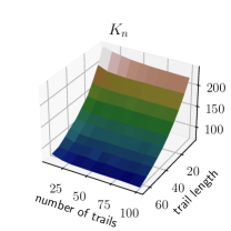
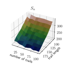
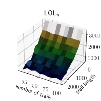
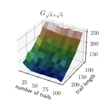
Figure 2: We measure the error $\|H-\hat{H}\|_{F}$ in the estimation of hitting times from trails for $n=16$ nodes on the complete graph ($K_{n}$), star graph ($S_{n}$), lollipop graph (LOL), and grid graph (GRID). We show the mean over $5$ runs. The cover time for the graphs are $16$, $46$, $612$, and $\approx 59.4$ respectively and we vary the trail length to a multiple of the cover time for each graph.

Table 2: Running times of different gradient implementations, over 1000 gradient descent iterations.

$n$	$5$	$10$	$50$	$1000$	$2000$
Analytical	$0.03\mathrm{s}\,\pm 0.01$	$\phantom{10}0.28\mathrm{s}\,\pm 0.01$	$1.41\mathrm{s}\,\pm 0.06$	$10.07\mathrm{m}\,\pm 0.19$	$76.33\mathrm{m}\,\pm 0.18$
Autodiff	$0.40\mathrm{s}\,\pm 0.02$	$100.40\mathrm{s}\,\pm 1.78$	$>2\mathrm{h}$	$>2\mathrm{h}$	$>2\mathrm{h}$
Numerical	$2.64\mathrm{s}\,\pm 0.10$	$164.67\mathrm{s}\,\pm 1.80$	$>2\mathrm{h}$	$>2\mathrm{h}$	$>2\mathrm{h}$

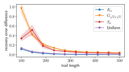
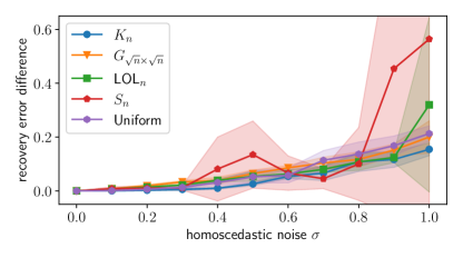
Figure 3: Learning Markov chains from noisy hitting times, for different graph types and noise levels. We plot the difference between the recovery error achieved by Wittmann et al. [2009] and our method. The difference is consistently positive, indicating an improvement for ULTRA-MC. On the left, the improvement for the lollipop graph LOL_n exceeds $50$, so we omit it from the plot.

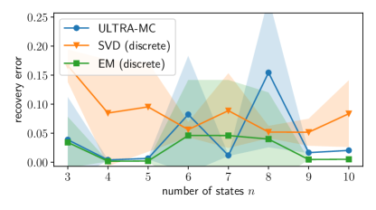
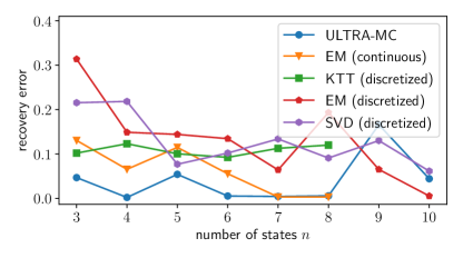
Figure 4: Learning a discrete-time (left) and continuous time (right) random mixture of $C=2$ chains from trails. We report average and standard deviation. Missing points indicate a timeout at 2 hours. For readability, we report the standard deviation separately in Table 3 of Appendix B

Figure 5: Three out of $C=6$ strategies of the Denver Nuggets. The remaining ones are in Figure 1. We mark the six positions in a basketball game: Point Guard (PG), Shooting Guard (SG), Power Forward (PF), Center (C), and Small Forward (SF). Each position is annoted with the average ball holding time. Arrow thickness and opacity reflect the probability of a pass, and we omit passes that occur with probability less than 0.2 for clarity. The player most likely to start a passing game is highlighted in blue. Attempted shots are indicated in red (miss) and green (score).

Estimating Hitting Times

To establish a baseline for our method, we need to understand how accurately we can deduce hitting times from a specific number of trails of certain length. We use the four graph types $K_{n}$, $S_{n}$, LOL_n, and $G_{\sqrt{n}\times\sqrt{n}}$ to assess the basic estimation of hitting times (cf. Algorithm 2). In Figure 2, we vary the number of trails and their lengths and quantify the error between the true hitting times matrix $H$ and estimations $\hat{H}$ via the Frobenius norm. We find that $K_{n}$ is easiest in terms of sampling, as all hitting times are identical and linear in $n$. In contrast, the star graph $S_{n}$ demands longer trails to achieve comparable accuracy, owing to the asymmetry in its hitting times. A grid displays similar behavior. Conversely, for the lollipop graph, much longer trails are necessary to observe an acceptable estimation error. Overall, we observe that the estimation accuracy depends on the underlying Markov chain and the magnitude and skew of the hitting times. The number of sampled trails and their length needs to be chosen accordingly.

Learning a Single Markov Chain

To understand how robust our learning algorithm is under noise, especially compared to the method of Wittmann et al. [2009], we apply both methods to noisy hitting times. We either estimating the hitting times from trails or add homoscedastic Gaussian noise. Specifically, we set $\hat{H}_{uv}=H_{uv}+N(0,\sigma^{2})$ for each $u\not=v$ independently. In Figure 3, we report the improvement in recovery error over the method of Wittmann et al. [2009], as a function of the length of the sampled trails and the standard deviation $\sigma$. We consistently improve, particularly when the noise stems from estimating hitting times from trails. Figures 8 and 9 in Appendix B show the recovery error for both approaches, and also with heteroscedastic noise.

We also study the scalability of our method. Table 2 shows execution times for various gradient implementations, applied to a single random discrete-time Markov chain. We compare analytical gradients utilizing the formulae detailed in Section 4, and the methods of automatic differentiation (Autodiff) and numerical analysis (forward difference method). We see that our exact analytical derivatives are crucial for scalability as the other two methods are not even scalable to $\approx 50$ nodes. Furthermore, Figure 7 of Appendix B shows the convergence behavior. On the left, we display recovery error and loss for a fixed number of $10\,000$ gradient descent iterations using the true hitting times $H$. We see that $10\,000$ iterations suffice for a relatively large number of states $n$, but more iterations are necessary when $n>500$. On the right, we show the convergence of our method from a random initialization. We see that within only a few thousand iterations, we reach and then improve the recovery error obtained by Wittmann et al. [2009].

Learning Mixtures

In Figure 4, we conduct experiments using $C=2$ chains for the discrete and continuous-time settings. In discrete-time, we learn with 1000 trails and for the more challenging continuous-time setting, we increase this to 5000 trails. Trails are of length 1000 in both scenarios. Notably, in the continuous-time setting, EM (continuous) and KTT (discretized) exceeded a duration of 2 hours, leading to a timeout. Our findings indicate that $\mathsf{ULTRA\!-\!MC}$ is able to match the performance in discrete-time and surpasses the performance in continuous-time of other competing approaches, demonstrating improved effectiveness and scalability. We evaluate our method on Markovletics Spaeh and Tsourakakis [2024] which unmixes offensive strategies from the passing game in the NBA. We showcase six strategies of the Denver Nuggets in Figures 1 and 5. We also include a mixture of offensive strategies of the Boston Celtics in Appendix B. Although the assumption that the passing game follows a stochastic Markov process is simplistic, it still gives us direct insights about the passing game.

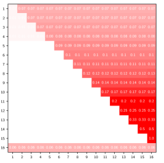
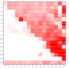
Figure 6: Learning a Markov chain on a complete DAG on $n=16$ nodes. The tables represent the transition matrices learned from the true hitting times (left) and noisy hitting times with $\sigma=0.3$ (right). Note that the true Markov chain has non-zero transition probabilities only for all $1\leq u<v\leq n$ where $M_{uv}=\frac{1}{n-u}$ and $M_{16,16}=1$.

Figure 10 shows the $C=6$ learned offensive strategies from Boston Celtics’ passing game during the 2022 season. The format of the plots shows the same format explain in Section 5.

Violating Irreducibility

In theory, our method requires aperiodic and irreducible chains in order to obtain Equation 1. Yet, Markov chains observed in practice may violate these conditions, such as cancer progression networks Beerenwinkel et al. [2005], Tsourakakis [2013], Desper et al. [1999]. To confirm that our approach is still practically applicable to such instances, we create trails from a directed acyclic graph (DAG) by adding every edge $(u,v)$ for $1\leq u<v\leq n$. For all pairs $u,v$, we calculate the estimated hitting times and assign a high value to the hitting time $H(u,v)$ whenever $u>v$. By setting the infinite hitting times to a value substantially greater than any observed hitting times, we effectively render the chain irreducible. This approach allows us to confirm that our algorithm can accurately learn the DAG structure by merely filtering out transitions with low probabilities.

We learn a Markov chain by replacing infinite hitting times with the value $100$, which is sufficiently large. As this introduces new, previously impossible transitions into the chain, we only retain transitions with sufficiently large mass. Specifically, if the transition probability from state $u$ to $v$ has probability $M_{uv}\leq 0.1\cdot\max_{w}M_{uw}$, we remove it from the chain. The results in Figure 6 indicate that in practical scenarios, we can circumvent the limitations of using our tools on irreducible chains by treating them as if they were irreducible, through assigning high values to the absent hitting times. A thorough investigation of this strategy merits its own dedicated study, which we aim to pursue as part of future research into understanding cancer progression through the use of mixed Markov chains Desper et al. [1999], Beerenwinkel et al. [2005].

6 Conclusion

In this work, we introduce $\mathsf{ULTRA\!-\!MC}$, a pioneering algorithm designed to efficiently learn either a single Markov chain or a mixture of Markov chains from a subset of potentially noisy hitting times. This is the first algorithm of its kind. Compelling questions to explore involve the development of more efficient and precise algorithms for learning mixtures. the design of improved estimators for deducing hitting times from trails, and better selection of the number of chains $C$.

Appendix A Omitted Algorithms and Proofs

A.1 Estimating Hitting Times

In Algorithm 2, we describe the estimation of hitting times from a set of trails $\mathbf{X}$. We state the algorithm in the discrete-time setting, but it naturally extends to the continuous-time setting as well. The algorithm is an efficient implementation of the following idea: For each trail $\mathbf{x}\in\mathbf{X}$, each index $t\in\mathbb{N}$ with state $\mathbf{x}_{t}=u$, and each other state $v\not=u$, we record the time $\min\{t^{\prime}\geq t:\mathbf{x}_{t^{\prime}}=v\}$ as a sample for the hitting time from $u$ to $v$. We then output the average over all these samples.

It is important to acknowledge that the method for estimating hitting times as outlined in Algorithm 2 carries a bias. This can be illustrated with a simple Markov chain example, containing two nodes, $u$ and $v$, where $v$ can be reached from $u$ through either a short or a long path. In scenarios where only the shorter path’s trajectories are observed due to the limited length of trails, and none from the longer path, the estimation might skew towards the shorter paths. In the case of a singular chain, this issue is manageable by linking paths together to simulate the longer journey, thus allowing for an unbiased estimation of hitting times. However, this strategy falls short in scenarios involving multiple chains because it relies on potentially inaccurate clustering, preventing seamless path concatenation without introducing further errors, as the original chain from which a trail is derived remains unknown. Consequently, in the context of estimating hitting times using Algorithm 2—especially when trails do not adequately cover long paths—the estimates are accepted to be biased. This method, however, avoids the pitfalls of adding errors through trail concatenation and still provides a reliable estimate of hitting times under these constraints.

In real-world scenarios, it might not always be possible to observe a transition from state $u$ to $v$. How we choose to handle the corresponding estimate $\hat{H}(u,v)$ can vary depending on the situation. In many of our experiments, we treat it as missing data, opting not to include it in our fitting process. In cases where we determine that a transition between these states is impossible, we assign it a significantly high value (e.g., Q6 in Section 5). For different applications, especially those where the observation period is short relative to the time needed for a transition, the development of right-censoring methods is advisable. Interestingly, the challenge of deriving hitting times from trails has yet to be thoroughly explored. The techniques described in Cherapanamjeri and Bartlett [2019], Daskalakis et al. [2018] may be beneficial in achieving this objective. It should be highlighted that the complexity of the issue decreases substantially when the trails are sufficiently lengthy, specifically of the order $\Omega(n^{3})$. This simplification can be demonstrated by employing concentration methods akin to those found in the works of Benjamini et al. [2006], Spaeh and Tsourakakis [2024]. It should be noted that although this issue is a classic one, the problem of deducing hitting times from trails of a specific length remains under-explored.

Algorithm 2 Estimating Hitting Times in discrete-time

  Input: Set of trails $\mathbf{X}$

  Output: Hitting times $\hat{H}$

  $T_{uv}\leftarrow 0$

  $C_{uv}\leftarrow 0$

  for each trail $\mathbf{x}\in\mathbf{X}$ do

     Initialize empty sequence $\texttt{P}_{u}$ for each $u\in V$

     for $t=1$ to $\mathrm{length}(\mathbf{x})$ do

        $u\leftarrow x_{t}$

        Append $t$ to $\texttt{P}_{u}$

     end for

     Let $i_{u}\leftarrow 1$ for each $u\in V$

     for $t=1$ to $\text{length}(\mathbf{x})$ do

        $u\leftarrow x_{t}$

        for $v\in V$ do

           if $i_{v}\leq\mathrm{length}(\texttt{P}_{v})$ then

              $T_{uv}\leftarrow T_{uv}+\texttt{P}_{v}(i_{v})-t$

              $C_{uv}\leftarrow C_{uv}+1$

           end if

        end for

     end for

  end for

  $\hat{H}_{uv}\leftarrow T_{uv}/C_{uv}$

A.2 Omitted Proofs

In this section, we give proofs and lemmas that we omitted in the main body. We start by showing the expression for the hitting times for discrete-time and continuous-time Markov chains in Section A.2.1. Next, we show how to obtain Lemmas 4.2 and 4.4 in Section A.2.2. The following Sections A.2.3 and A.2.4 contains Lemmas detailing the Jacobian of the stationary distribution and the Laplacian, respectively.

A.2.1 Hitting Times

Lemma A.1.

The hitting time from state $u$ to state $v$ for a discrete-time Markov chain with Laplacian $L$ is given by

$$H_{uv}=\left(\mathbf{1}-\frac{1}{s_{v}}\mathbf{1}_{v}\right)^{\top}L^{+}\left(\mathbf{1}_{u}-\mathbf{1}_{v}\right).$$

For completeness, we repeat the proof due to Cohen et al. [2016].

Proof.

For two states $u,v\in[n]$ we either have $H_{uv}=0$ if $u=v$ or, by the law of total expectation,

$$H_{uv}=\sum_{w}(1+H_{wv})M_{uw}=1+(MH)_{uv}.$$ (3)

We now fix $v$ and let $I=V\setminus\{v\}$. Then, (3) over all states $u$ is equivalent to

$$\begin{pmatrix}L_{I,I}&L_{I,v}\\ 0&1\end{pmatrix}\cdot\begin{pmatrix}H_{I,v}\\ H_{v,v}\end{pmatrix}=\begin{pmatrix}1\\ 0\end{pmatrix}.$$

We can construct a solution to this system: Let $d=\mathbf{1}-\frac{1}{s_{v}}\mathbf{1}_{v}$ such that $d^{\top}s=0$ Let $x$ be any solution to $Lx=d$ and note that $x$ is unique up to adding multiples of $\mathbf{1}$. Therefore, $y=x-x_{v}\mathbf{1}$ is a solution with $Ly=d$ and $y_{v}=\mathbf{0}$ and $y$ therefore satisfies the above linear system. Due to uniqueness, $H_{u,v}=y_{u}$ and

$$H_{uv}=y_{u}=\mathbf{1}_{u}^{\top}\underbrace{L^{+}d}_{=x}-\underbrace{\mathbf{1}_{v}^{\top}L^{+}d}_{=x_{v}}=\left(\mathbf{1}_{u}-\mathbf{1}_{v}\right)^{\top}L^{+}\underbrace{\left(\mathbf{1}-\frac{1}{s_{v}}\mathbf{1}\right)}_{=d}.$$

∎

There is no analog expression for CTMCs. We state such an extension as the following lemma.

Lemma A.2.

The hitting time from state $u$ to state $v$ for a continuous-time Markov chain with rate matrix $K$ is given by

$$H_{uv}=\left(\mathbf{1}-\frac{1}{s_{v}}\mathbf{1}_{v}\right)^{\top}(-K)^{+}\left(\mathbf{1}_{u}-\mathbf{1}_{v}\right).$$

Proof.

We derive the result analogously to Lemma A.1. Recall that in a continuous-time Markov chain the transition probabilities are given as the matrix exponential $M(\tau)=e^{\tau K}$. Let now $H(\tau)$ be the hitting times in $M(\tau)$ and note that $H=\lim_{\tau\to 0}H(\tau)$. In the chain $M(\tau)$, we again obtain through the law of total expectation that

$$H(\tau)_{uv}=\tau+\sum_{w}H(\tau)_{w,v}M(\tau)$$

for states $u\not=v$. Note that this is just a scaled version of (3) in the proof of Lemma A.1, The solution to this system is therefore a scaled version of the solution to (3), i.e.

$$H(\tau)_{uv}=\tau\left(\mathbf{1}-\frac{1}{s_{v}}\mathbf{1}_{v}\right)^{\top}L(\tau)^{+}\left(\mathbf{1}_{u}-\mathbf{1}_{v}\right)$$

where $L(\tau)=I-M(\tau)$. Finally,

$$H_{uv} =\lim_{\tau\to 0}H(\tau)_{uv}$$

$$=\lim_{\tau\to 0}\tau\left(\mathbf{1}-\frac{1}{s_{v}}\mathbf{1}_{v}\right)^{\top}L(\tau)^{+}\left(\mathbf{1}_{u}-\mathbf{1}_{v}\right)$$

$$=\left(\mathbf{1}-\frac{1}{s_{v}}\mathbf{1}_{v}\right)^{\top}\left(\lim_{\tau\to 0}\frac{1}{\tau}L(\tau)\right)^{+}\left(\mathbf{1}_{u}-\mathbf{1}_{v}\right)$$

$$=\left(\mathbf{1}-\frac{1}{s_{v}}\mathbf{1}_{v}\right)^{\top}(-K)^{+}\left(\mathbf{1}_{u}-\mathbf{1}_{v}\right)$$

as $\frac{1}{\tau}L(\tau)=\frac{1}{\tau}(I-e^{\tau K})\to-K$ for $\tau\to 0$. ∎

A.2.2 Computing the Gradient of the Loss

We now complete the derivation of the efficient gradient expression from Section 4.1. We begin by proving Lemma 4.3 which we need to compute the stationary distribution and its derivative.

Lemma 4.1. Let $a=\mathbf{1}^{\top}L^{+}\in\mathbb{R}^{1\times n}$ and set

$$A =a^{\top}\mathbf{1}^{\top}-\mathbf{1}a$$

$$B =\left(L^{+}-\mathrm{diag}\left(L^{+}\right)\mathbf{1}^{\top}\right)^{\top}\mathrm{diag}\left(s\right)^{-1}.$$

Then, $H=A-B$.

Proof.

Pick a pair of states $u,v\in[n]$. We can re-write Equation (1) as

$$H_{uv}=\mathbf{1}^{\top}L^{+}\chi_{vu}-\frac{1}{s_{v}}e_{v}^{\top}L^{+}\chi_{vu}.$$ (4)

The first term evaluates to $\mathbf{1}^{\top}L^{+}\chi_{vu}=a_{u}-a_{v}=A_{uv}.$ The second term is

$$\frac{1}{s_{v}}e_{v}^{\top}L^{+}\chi_{vu} =\frac{1}{s_{v}}\left(L_{vu}^{+}-L_{vv}^{+}\right)$$

$$=\frac{1}{s_{v}}\left(L^{+}-\mathrm{diag}\left(L^{+}\right)\mathbf{1}^{\top}\right)_{vu}$$

$$=\left(\left(L^{+}-\mathrm{diag}\left(L^{+}\right)\mathbf{1}^{\top}\right)^{\top}\mathrm{diag}\left(s\right)^{-1}\right)_{uv}=B_{uv}$$

∎

Lemma 4.3. The stationary distribution for a Markov chain with Laplacian $L$ is $s=\frac{d}{\|d\|_{1}}$ where $d=\mathbf{1}-LL^{+}\mathbf{1}$.

Proof.

The stationary distribution is the probability vector $s\in\Delta_{n}$ such that $s_{u}=\sum_{v}M_{vu}s_{v}$ for all $u\in[n]$. The latter is equivalent to $s^{\top}=s^{\top}M$ or $s^{\top}L=\mathbf{0}$. Note that $LL^{+}$ is symmetric, and therefore

$$d^{\top}L=\mathbf{1}^{\top}L-\mathbf{1}^{\top}(LL^{+})^{\top}L=\mathbf{1}^{\top}L-\mathbf{1}^{\top}LL^{+}L.$$

By properties of the pseudoinverse, $LL^{+}L=L$ and thus $d^{\top}L=\mathbf{0}$ which implies $s^{\top}L=\frac{1}{\|d\|_{1}}d^{\top}L=\mathbf{0}$. It remains to show that $s\in\Delta_{n}$, for which we need that $d\geq\mathbf{0}$ (coordinate-wise). By definition of $d$, the latter is equivalent to $\mathbf{1}\geq LL^{+}\mathbf{1}$. It is well known that $LL^{+}$ is an orthogonal projection and thus has eigenvalues either $0$ or $1$ and therefore, all entries of $LL^{+}\mathbf{1}$ have value at most $1$. ∎

Recall that we split the computation of the gradient into two terms

$$\nabla\ell_{2}(L^{+})=\left(\frac{\partial A}{\partial L^{+}}\right)^{\top}\otimes\Delta+\left(\frac{\partial B}{\partial L^{+}}\right)^{\top}\otimes\Delta$$

We now prove Lemmas 4.2 and 4.4 which give expressions for both terms.

Lemma 4.2. We have

$$\left(\frac{\partial A}{\partial L^{+}}\right)^{\top}\otimes\Delta=\mathbf{1}\left(\mathbf{1}^{\top}\Delta\right)-\left(\mathbf{1}^{\top}\Delta\right)^{\top}\mathbf{1}^{\top}-\mathbf{1}\left(\Delta\mathbf{1}\right)^{\top}+\left(\Delta\mathbf{1}\right)\mathbf{1}^{\top}.$$

Furthermore, $\left(\frac{\partial A}{\partial L^{+}}\right)^{\top}\otimes\Delta$ can be computed in time $O(n^{2})$.

Proof.

Note that

$$\frac{\partial A}{\partial L_{uv}^{+}}=\frac{\partial}{\partial L_{uv}^{+}}\left(a^{\top}\mathbf{1}^{\top}-\mathbf{1}a\right)=\frac{\partial}{\partial L_{uv}^{+}}\left(L^{\top+}\mathbf{1}\mathbf{1}^{\top}-\mathbf{1}\mathbf{1}^{\top}L^{+}\right)=\frac{\partial}{\partial L_{uv}^{+}}\left(\left(\mathbf{1}\mathbf{1}^{\top}L^{+}\right)^{\top}-\mathbf{1}\mathbf{1}^{\top}L^{+}\right).$$

Recall that $\frac{\partial L^{+}}{\partial L^{+}_{uv}}=\mathbf{1}\chi_{vu}^{\top}$ which implies

$$\frac{\partial}{\partial L_{uv}^{+}}\mathbf{1}\mathbf{1}^{\top}L^{+}=\mathbf{1}\chi_{vu}^{\top}$$

and thus

$$\frac{\partial A}{\partial L_{uv}^{+}}=\chi_{vu}\mathbf{1}^{\top}-\mathbf{1}\chi_{vu}^{\top}.$$

Finally,

$$\mathbf{1}^{\top}\left(\left(\frac{\partial A}{\partial L_{uv}^{+}}\right)\circ\Delta\right)\mathbf{1}=\mathbf{1}^{\top}\left(\mathbf{1}\left(e_{v}^{\top}-e_{u}^{\top}\right)\circ\Delta-\chi_{vu}\mathbf{1}^{\top}\circ\Delta\right)\mathbf{1}\\ =\mathbf{1}^{\top}\left(\mathbf{1}\left(e_{v}^{\top}-e_{u}^{\top}\right)\circ\Delta\right)\mathbf{1}-\mathbf{1}^{\top}\left(\chi_{vu}\mathbf{1}^{\top}\circ\Delta\right)\mathbf{1}=\left(\mathbf{1}^{\top}\Delta\right)_{v}-\left(\mathbf{1}^{\top}\Delta\right)_{u}-\left(\Delta\mathbf{1}\right)_{v}+\left(\Delta\mathbf{1}\right)_{u}$$

and thus

$$\left(\frac{\partial A}{\partial L^{+}}\right)^{\top}\otimes\Delta=\left(\left(\mathbf{1}^{\top}\Delta\right)_{v}-\left(\mathbf{1}^{\top}\Delta\right)_{u}-\left(\Delta\mathbf{1}\right)_{v}+\left(\Delta\mathbf{1}\right)_{u}\right)_{uv}\\ =\mathbf{1}\left(\mathbf{1}^{\top}\Delta\right)-\left(\mathbf{1}^{\top}\Delta\right)^{\top}\mathbf{1}^{\top}-\mathbf{1}\left(\Delta\mathbf{1}\right)^{\top}+\left(\Delta\mathbf{1}\right)\mathbf{1}^{\top}.$$

Note that this term only involves summing over rows and columns, which can be done in $O(n^{2})$. ∎

Lemma 4.4. We have

$$\left(\frac{\partial B}{\partial L^{+}}\right)^{\top}\otimes\Delta=\mathrm{diag}(s)^{-1}\mathbf{1}\mathbf{1}^{\top}(\Delta^{\top}-\Delta)+\Delta\mathrm{diag}(s)^{-1}\mathbf{1}\mathbf{1}^{\top}+G$$

for

$$G=\left(\mathbf{1}^{\top}\left(\left(L^{+}-\mathrm{diag}\left(L^{+}\right)\mathbf{1}^{\top}\right)^{\top}D\circ\Delta\right)g_{uv}\right)_{uv}.$$

Furthermore, $\left(\frac{\partial B}{\partial L^{+}}\right)^{\top}\otimes\Delta$ can be computed in time $O(n^{3})$.

Proof.

We pick a pair of states $u\not=v$. By definition of $B$ and the product rule,

$$\frac{\partial B}{\partial L_{uv}^{+}} =\frac{\partial}{\partial L_{uv}^{+}}\left(L^{+}-\mathrm{diag}\left(L^{+}\right)\mathbf{1}^{\top}\right)^{\top}\mathrm{diag}\left(s\right)^{-1}$$

$$=\left(\frac{\partial}{\partial L_{uv}^{+}}\left(L^{+}-\mathrm{diag}\left(L^{+}\right)\mathbf{1}^{\top}\right)^{\top}\right)\mathrm{diag}\left(s\right)^{-1}$$ (5)

$$\quad+\left(L^{+}-\mathrm{diag}\left(L^{+}\right)\mathbf{1}^{\top}\right)^{\top}\left(\frac{\partial}{\partial L_{uv}^{+}}\mathrm{diag}\left(s\right)^{-1}\right).$$ (6)

We consider the two terms (5) and (6) separately. To obtain (5), we calculate

$$\frac{\partial}{\partial L_{uv}^{+}}\left(L^{+}-\mathrm{diag}\left(L^{+}\right)\mathbf{1}^{\top}\right)=\mathbf{1}\chi_{vu}^{\top}+e_{u}\mathbf{1}^{\top}$$

and thus have that

$$\eqref{eq:fst}=\left(\mathbf{1}\chi_{vu}^{\top}+e_{u}\mathbf{1}^{\top}\right)\mathrm{diag}(s)^{-1}.$$

For (6), we use Lemma A.3 and obtain

$$\frac{\partial}{\partial L_{uv}^{+}}\mathrm{diag}\left(s\right)^{-1} =\mathrm{diag}\left(\left(\frac{1}{d_{w}}\left(\frac{\|d\|_{1}}{d_{w}}e_{w}^{\top}-\mathbf{1}^{\top}\right)g_{uv}\right)_{w}\right)$$

$$=\mathrm{diag}\left(g_{uv}\right)D.$$

for $D=\mathrm{diag}\left(\left(\frac{1}{d_{w}}\left(\frac{1}{s_{w}}e_{w}^{\top}-\mathbf{1}^{\top}\right)\right)_{w}\right)$. Thus,

$$\eqref{eq:snd}=\left(L^{+}-\mathrm{diag}\left(L^{+}\right)\mathbf{1}^{\top}\right)^{\top}\mathrm{diag}(g_{uv})D.$$

and overall, for $s^{-1}=(s^{-1}_{w})_{w}$,

$$\mathbf{1}^{\top}\left(\frac{\partial B}{\partial L^{+}_{uv}}\circ\Delta\right)\mathbf{1} =\mathbf{1}^{\top}\left(\left(\mathbf{1}\chi_{vu}^{\top}+e_{u}\mathbf{1}^{\top}\right)\mathrm{diag}\left(s\right)^{-1}\circ\Delta\right)\mathbf{1}$$

$$\quad+\mathbf{1}^{\top}\left(\left(L^{+}-\mathrm{diag}\left(L^{+}\right)\mathbf{1}^{\top}\right)^{\top}\mathrm{diag}(g_{uv})D\circ\Delta\right)\mathbf{1}$$

$$=\mathbf{1}^{\top}\left(\mathbf{1}\chi_{vu}^{\top}\circ\Delta+e_{u}\mathbf{1}^{\top}\circ\Delta\right)s^{-1}$$

$$\quad+\mathbf{1}^{\top}\left(\left(L^{+}-\mathrm{diag}\left(L^{+}\right)\mathbf{1}^{\top}\right)^{\top}D\circ\Delta\right)g_{uv}$$

$$=\frac{1}{s_{v}}\left(\mathbf{1}^{\top}\Delta\right)_{v}-\frac{1}{s_{u}}\left(\mathbf{1}^{\top}\Delta\right)_{u}+e_{u}^{\top}\Delta s^{-1}$$

$$\quad+\mathbf{1}^{\top}\left(\left(L^{+}-\mathrm{diag}\left(L^{+}\right)\mathbf{1}^{\top}\right)^{\top}D\circ\Delta\right)g_{uv}$$

where the second equality holds because $\mathrm{diag}(g_{uv})$ and $\mathrm{diag}(s)$ are diagonal. Therefore,

$$\left(\frac{\partial B}{\partial L^{+}_{uv}}\right)^{\top}\otimes\Delta =\left(\mathrm{diag}(s)^{-1}\mathbf{1}\mathbf{1}^{\top}\Delta\right)^{\top}-\mathrm{diag}(s)^{-1}\mathbf{1}\mathbf{1}^{\top}\Delta+\Delta\mathrm{diag}(s)^{-1}\mathbf{1}\mathbf{1}^{\top}+G$$

$$=\mathrm{diag}(s)^{-1}\mathbf{1}\mathbf{1}^{\top}(\Delta^{\top}-\Delta)+\Delta\mathrm{diag}(s)^{-1}\mathbf{1}\mathbf{1}^{\top}+G.$$

Note that we can clearly compute $\mathrm{diag}(s)^{-1}\mathbf{1}\mathbf{1}^{\top}(\Delta^{\top}-\Delta)$ and $\Delta\mathrm{diag}(s)^{-1}\mathbf{1}^{\top}\mathbf{1}$ in time $O(n^{3})$. It remains to show that $G$ can be computed in time $O(n^{3})$: Note that we can pre-compute the vector

$$\mathbf{1}^{\top}\left(\left(L^{+}-\mathrm{diag}\left(L^{+}\right)\mathbf{1}^{\top}\right)^{\top}D\circ\Delta\right)$$

in time $O(n^{3})$. Furthermore, since

$$g_{uv}=e_{u}\chi_{vu}^{\top}(LL^{+}+I)\mathbf{1},$$

we can also pre-compute the vector $(LL^{+}+I)\mathbf{1}$ and then determine $g_{uv}$ in time $O(n)$ for each $u,v\in[n]$. Finally, we can compute each inner product to obtain the entry $G_{uv}$ in time $O(n)$, so overall we need $O(n^{3})$ to compute $G$. ∎

A.2.3 Jacobian of the Stationary Distribution

Lemma A.3.

For any pair $u\not=v$ and state $w$,

$$\frac{\partial s_{w}^{-1}}{\partial L_{uv}^{+}}=\frac{1}{d_{w}}\left(\frac{1}{s_{w}}e_{w}^{\top}-\mathbf{1}^{\top}\right)Lg_{uv}$$

where $g_{uv}=e_{u}\chi_{vu}^{\top}(LL^{+}+I)\mathbf{1}$.

Proof.

Recall that $s=\frac{d}{\|d\|_{1}}$ for $d=\mathbf{1}-LL^{+}\mathbf{1}$. Let us thus first calculate $\frac{\partial d}{\partial L^{+}_{uv}}$. We have

$$\frac{\partial d}{\partial L_{uv}^{+}}=\frac{\partial}{\partial L_{uv}^{+}}\left(\mathbf{1}-LL^{+}\mathbf{1}\right)=-\frac{\partial}{\partial L_{uv}^{+}}LL^{+}\mathbf{1}\\ =-\left(\frac{\partial L}{\partial L_{uv}^{+}}\right)L^{+}\mathbf{1}-L\left(\frac{\partial L^{+}}{\partial L_{uv}^{+}}\right)\mathbf{1}=-Le_{u}\chi_{vu}^{\top}LL^{+}\mathbf{1}-Le_{u}\chi_{vu}^{\top}\mathbf{1}=-L\underbrace{e_{u}\chi_{vu}^{\top}(LL^{+}+I)\mathbf{1}}_{=g_{uv}}$$

where we use Corollary A.5 to evaluate $\left(\frac{\partial L}{\partial L^{+}_{uv}}\right)L^{+}\mathbf{1}$. Since $d\geq\mathbf{0}$, we furthermore obtain for the length that

$$\frac{\partial}{\partial L_{uv}^{+}}\|d\|_{1}=\frac{\partial}{\partial L_{uv}^{+}}\mathbf{1}^{\top}d=\mathbf{1}^{\top}\frac{\partial d}{\partial L_{uv}^{+}}=-\mathbf{1}^{\top}Lg_{uv}.$$

Given this, we can now proceed to calculate the Jacobian of the stationary distribution. We use the product rule to decompose

$$\frac{\partial s_{w}^{-1}}{\partial L_{uv}^{+}}=\frac{\partial}{\partial L_{uv}^{+}}\frac{\|d\|_{1}}{d_{w}}=\frac{1}{d_{w}}\left(\frac{\partial}{\partial L_{uv}^{+}}\|d\|_{1}\right)-\frac{\|d\|_{1}}{d_{w}^{2}}\left(\frac{\partial d_{w}}{\partial L_{uv}^{+}}\right).$$

We plug in our previous calculations for $d$ and obtain

$$\frac{\partial s_{w}^{-1}}{\partial L_{uv}^{+}}=\left(-\frac{1}{d_{w}}\mathbf{1}^{\top}+\frac{\|d\|_{1}}{d_{w}^{2}}e_{w}^{\top}\right)Lg_{uv}=\frac{1}{d_{w}}\left(\frac{1}{s_{w}}e_{w}^{\top}-\mathbf{1}^{\top}\right)Lg_{uv}.$$

∎

A.2.4 Jacobian of the Laplacian

Lemma A.4.

The Laplacian has the following Jacobian with respect to $L^{+}_{uv}$, for any $u\not=v$:

$$\frac{\partial L}{\partial L^{+}_{uv}}=LL^{\top}\chi_{vu}e_{u}^{\top}\left(I-L^{+}L\right)-Le_{u}\chi_{vu}^{\top}L.$$

Proof.

We want to evaluate the matrix $\frac{\partial L}{\partial L^{+}_{uv}}$ in closed form. Let $X=L^{+}$ and note that $L=X^{+}$. By the definition of the gradient,

$$\frac{\partial X^{+}}{\partial X_{uv}}=\lim_{\epsilon\to 0}\frac{1}{\epsilon}((X+\epsilon e_{u}\chi_{vu}^{\top})^{+}-X^{+}).$$ (7)

We can use a result from Meyer [1973] to evaluate the rank-one update $X+\epsilon e_{u}\chi_{vu}^{\top}$ to the pseudoinverse. Note that we meet the preconditions of Theorem 5 from Meyer [1973]: First, $\chi_{vu}$ is in the row space of $X=L^{+}$. This is true since $L^{+}$ has rank $n-1$, the kernel of the row space of $L^{+}$ is spanned by $\mathbf{1}^{\top}$ since $\mathbf{1}^{\top}L^{+}=\mathbf{0}$, and $\chi_{vu}$ is orthogonal to $\mathbf{1}$. Second, we require that $\beta=1+\epsilon\chi_{vu}X^{+}e_{u}\not=0$. Clearly, $\beta>0$ for sufficiently small $\epsilon$. We can thus apply Theorem 5 from Meyer [1973] and get

$$(X+\epsilon e_{u}\chi_{vu}^{\top})^{+}=X^{+}+\epsilon\frac{1}{\beta}X^{+}h^{\top}u^{\top}-\epsilon\frac{\beta}{\sigma}pq^{\top}$$

where

$$\beta =1+\epsilon\chi_{vu}^{\top}X^{+}e_{u}\in\mathbb{R}$$

$$h =\chi_{vu}^{\top}X^{+}\in\mathbb{R}^{1\times n}$$

$$u =\left(I-XX^{+}\right)e_{u}\in\mathbb{R}^{n}$$

$$k =X^{+}e_{u}\in\mathbb{R}^{n}$$

$$p =-\epsilon\frac{\|u\|^{2}}{\beta}X^{+}h^{\top}-k\in\mathbb{R}^{n}$$

$$q^{\top} =-\epsilon\frac{\|h\|^{2}}{\beta}u^{\top}-h\in\mathbb{R}^{1\times n}$$

$$\sigma =\epsilon^{2}\|h\|^{2}\cdot\|u\|^{2}+\left|\beta\right|^{2}\in\mathbb{R}$$

We plug this back into (7) and obtain

$$\frac{\partial X^{+}}{\partial X_{uv}}=\lim_{\epsilon\to 0}\frac{1}{\beta}X^{+}h^{\top}u^{\top}-\lim_{\epsilon\to 0}\frac{\beta}{\sigma}pq^{\top}$$ (8)

We treat both limits separately. For the first limit, we have

$$\lim_{\epsilon\to 0}\frac{1}{\beta}X^{+}h^{\top}u^{\top}=\left(\lim_{\epsilon\to 0}\frac{1}{1+\epsilon\chi_{vu}^{\top}X^{+}e_{u}}\right)X^{+}h^{\top}u^{\top}=X^{+}h^{\top}u^{\top}=X^{+}X^{\top+}\chi_{vu}e_{u}^{\top}(I-XX^{+})^{\top}.$$

as only $\beta$ depends on $\epsilon$. For the second term in (8), we compute

$$\lim_{\epsilon\to 0}\frac{\beta}{\sigma}pq^{\top}=kh=X^{+}e_{u}\chi_{vu}^{\top}X^{+}$$

since $\frac{\beta}{\sigma}\to 1$, $p\to-k$ and $q^{\top}\to-h$ for $\epsilon\to 0$. We plug this back into (8) to obtain that overall,

$$\frac{\partial X^{+}}{\partial X_{uv}}=X^{+}X^{\top+}\chi_{vu}e_{u}^{\top}(I-XX^{+})^{\top}-X^{+}e_{u}\chi_{vu}^{\top}X^{+}.$$

The final statement follows as $XX^{+}$ is symmetric. ∎

Corollary A.5.

For any $u\not=v$,

$$\left(\frac{\partial L}{\partial L_{uv}^{+}}\right)L^{+}\mathbf{1}=LL^{\top}\chi_{uv}e_{u}^{\top}\mathbf{1}.$$

Proof.

By properties of the pseudoinverse, $(I-L^{+}L)L^{+}\mathbf{1}=L^{+}\mathbf{1}-L^{+}LL^{+}\mathbf{1}=L^{+}\mathbf{1}-L^{+}\mathbf{1}=\mathbf{0}$. We use this to simplify the Jacobian obtained in Lemma A.4:

$$\left(\frac{\partial L}{\partial L_{uv}^{+}}\right)L^{+}\mathbf{1}=LL^{\top}\chi_{vu}e_{u}^{\top}\left(I-L^{+}L\right)L^{+}\mathbf{1}-Le_{u}\chi_{vu}^{\top}LL^{+}\mathbf{1}=Le_{u}\chi_{uv}^{\top}LL^{+}\mathbf{1}.$$

∎

Appendix B Additional Experimental Results

We present the experimental results that we omitted from the main body due to space constraints.

Figure 7 shows the convergence behavior of our gradient descent approach for learning a single Markov chain. We show the recovery error for a fixed number of iterations and the recovery error per iteration, compared to the recovery error achieved by Wittmann et al. [2009]. As we observe in Figure 7 (left), the number of iterations should depend on the number of states. We observe a sudden transition in the loss function that translates to a sudden transition to the recovery error as well from 450 to 500 states. For $n=25$ states, we observe in Figure 7 (right) that a few thousand iterations suffice to obtain a good solution. After 1000 iterations our obtained solution always improves the solution found by Wittman et al. Wittmann et al. [2009] and occassionally even 500 iterations suffice.

Figures 8 and 9 show the recovery error of our approach and the approach of Wittmann et al. [2009], for which we reported the difference in Figure 3. We also show results with heteroscedastic noise in Figure 9. In this scenario, the noise level $\sigma_{uv}$ is proportional to $\sigma(H(u,v))$, with $\sigma_{uv}=2\cdot H(u,v)/t_{\text{cover}}$, where $t_{\text{cover}}$ is the cover time of the underlying Markov chain. The observed trend continues to be approximately linear, mirroring the pattern observed with homoscedastic noise.

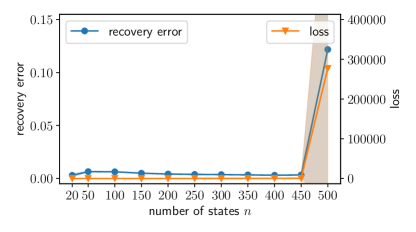
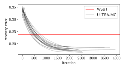
Figure 7: (Left) Learning a single transition matrix $M$ from hitting times using $10\,000$ gradient descent iterations. (Right) Convergence of $\mathsf{ULTRA\!-\!MC}$ from a random initialization compared with the method of Wittmann et al. [2009] (WSBT), for a uniform random Markov chain on $n=25$ states and homoscedastic noise with $\sigma=0.5$.

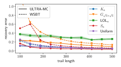
Figure 8: Learning Markov chains via hitting times estimated from trails.

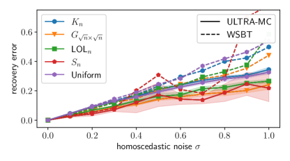
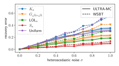
Figure 9: Learning Markov chains under homoscedastic and heteroscedastic noise.

Figure 10: Offensive strategies of the Boston Celtics during the 2022 season, learned from a mixture of $C=6$ continuous-time Markov chains.

Table 3: Empirical standard deviation of the results in Figure 4

$n$	3	4	5	6	7	8	9	10
ULTRA-MC	0.04	0.0	0.11	0.0	0.0	0.0	0.15	0.08
EM (continuous)	0.08	0.06	0.15	0.08	0.0	0.0
KTT (discretized)	0.03	0.04	0.03	0.03	0.02	0.01
EM (discretized)	0.18	0.2	0.19	0.18	0.13	0.17	0.14	0.0
SVD (discretized)	0.16	0.15	0.13	0.13	0.16	0.08	0.13	0.07

References

- sec [2024] Second spectrum. https://www.secondspectrum.com, 2024. [Online; accessed 16-May-2024].
- Anandkumar et al. [2012] Animashree Anandkumar, Daniel Hsu, and Sham M Kakade. A method of moments for mixture models and hidden markov models. In Conference on Learning Theory, pages 33–1. JMLR Workshop and Conference Proceedings, 2012.
- Anandkumar et al. [2014] Animashree Anandkumar, Rong Ge, Daniel Hsu, Sham M Kakade, and Matus Telgarsky. Tensor decompositions for learning latent variable models. Journal of machine learning research, 15:2773–2832, 2014.
- Beerenwinkel et al. [2005] Niko Beerenwinkel, Jörg Rahnenführer, Rolf Kaiser, Daniel Hoffmann, Joachim Selbig, and Thomas Lengauer. Mtreemix: a software package for learning and using mixture models of mutagenetic trees. Bioinformatics, 21(9):2106–2107, 2005.
- Benjamini et al. [2006] Itai Benjamini, Gady Kozma, László Lovász, Dan Romik, and Gabor Tardos. Waiting for a bat to fly by (in polynomial time). Combinatorics, Probability and Computing, 15(5):673–683, 2006.
- Blanchet et al. [2016] Jose Blanchet, Guillermo Gallego, and Vineet Goyal. A markov chain approximation to choice modeling. Operations Research, 64(4):886–905, 2016.
- Brightwell and Winkler [1990] Graham Brightwell and Peter Winkler. Maximum hitting time for random walks on graphs. Random Structures & Algorithms, 1(3):263–276, 1990.
- Cherapanamjeri and Bartlett [2019] Yeshwanth Cherapanamjeri and Peter L Bartlett. Testing symmetric markov chains without hitting. In Conference on Learning Theory, pages 758–785. PMLR, 2019.
- Chierichetti et al. [2012] Flavio Chierichetti, Ravi Kumar, Prabhakar Raghavan, and Tamas Sarlos. Are web users really markovian? In Proceedings of the 21st international conference on World Wide Web, pages 609–618, 2012.
- Chierichetti et al. [2018] Flavio Chierichetti, Ravi Kumar, and Andrew Tomkins. Learning a mixture of two multinomial logits. In International Conference on Machine Learning, pages 961–969. PMLR, 2018.
- Cohen et al. [2016] Michael B. Cohen, Jonathan A. Kelner, John Peebles, Richard Peng, Aaron Sidford, and Adrian Vladu. Faster algorithms for computing the stationary distribution, simulating random walks, and more. In FOCS, pages 583–592. IEEE Computer Society, 2016.
- Dasgupta [1999] Sanjoy Dasgupta. Learning mixtures of gaussians. In 40th Annual Symposium on Foundations of Computer Science (Cat. No. 99CB37039), pages 634–644. IEEE, 1999.
- Daskalakis et al. [2018] Constantinos Daskalakis, Nishanth Dikkala, and Nick Gravin. Testing symmetric markov chains from a single trajectory. In Conference On Learning Theory, pages 385–409. PMLR, 2018.
- Deisenroth et al. [2020] Marc Peter Deisenroth, A Aldo Faisal, and Cheng Soon Ong. Mathematics for machine learning. Cambridge University Press, 2020.
- Dempster et al. [1977] Arthur P Dempster, Nan M Laird, and Donald B Rubin. Maximum likelihood from incomplete data via the em algorithm. Journal of the Royal Statistical Society: Series B (Methodological), 39(1):1–22, 1977.
- Desper et al. [1999] Richard Desper, Feng Jiang, Olli-P Kallioniemi, Holger Moch, Christos H Papadimitriou, and Alejandro A Schäffer. Inferring tree models for oncogenesis from comparative genome hybridization data. Journal of computational biology, 6(1):37–51, 1999.
- Donoho and Gavish [2013] David L Donoho and Matan Gavish. The optimal hard threshold for singular values is 4/sqrt (3). arXiv preprint arXiv:1305.5870, 2013.
- Efron and Tibshirani [1991] Bradley Efron and Robert Tibshirani. Statistical data analysis in the computer age. Science, 253(5018):390–395, 1991.
- Fearon and Vogelstein [1990] Eric R Fearon and Bert Vogelstein. A genetic model for colorectal tumorigenesis. cell, 61(5):759–767, 1990.
- Feige [1995] Uriel Feige. A tight upper bound on the cover time for random walks on graphs. Random structures and algorithms, 6(1):51–54, 1995.
- Gordon et al. [2021] Spencer L Gordon, Bijan Mazaheri, Yuval Rabani, and Leonard J Schulman. Identifying mixtures of bayesian network distributions. arXiv preprint arXiv:2112.11602, 2021.
- Gupta et al. [2016] Rishi Gupta, Ravi Kumar, and Sergei Vassilvitskii. On mixtures of markov chains. Advances in neural information processing systems, 29, 2016.
- Hoskins et al. [2018] Jeremy G Hoskins, Cameron Musco, Christopher Musco, and Charalampos E Tsourakakis. Learning networks from random walk-based node similarities. arXiv preprint arXiv:1801.07386, 2018.
- Jolliffe and Cadima [2016] Ian T Jolliffe and Jorge Cadima. Principal component analysis: a review and recent developments. Philosophical transactions of the royal society A: Mathematical, Physical and Engineering Sciences, 374(2065):20150202, 2016.
- Kausik et al. [2023] Chinmaya Kausik, Kevin Tan, and Ambuj Tewari. Learning mixtures of Markov chains and MDPs. In Andreas Krause, Emma Brunskill, Kyunghyun Cho, Barbara Engelhardt, Sivan Sabato, and Jonathan Scarlett, editors, Proceedings of the 40th International Conference on Machine Learning, volume 202 of Proceedings of Machine Learning Research, pages 15970–16017. PMLR, 23–29 Jul 2023. URL https://proceedings.mlr.press/v202/kausik23a.html.
- Kingma and Ba [2015] Diederik P. Kingma and Jimmy Ba. Adam: A method for stochastic optimization. In ICLR (Poster), 2015.
- Kodinariya et al. [2013] Trupti M Kodinariya, Prashant R Makwana, et al. Review on determining number of cluster in k-means clustering. International Journal, 1(6):90–95, 2013.
- Lafferty and Zhai [2001] John Lafferty and Chengxiang Zhai. Document language models, query models, and risk minimization for information retrieval. In Proceedings of the 24th annual international ACM SIGIR conference on Research and development in information retrieval, pages 111–119, 2001.
- Levin et al. [2017] David A Levin, Elizabeth Wilmer, and Yuval Peres. Markov chains and mixing times, volume 107. American Mathematical Soc., 2017.
- Lindsay [1995] Bruce G Lindsay. Mixture models: theory, geometry, and applications. Ims, 1995.
- McGibbon and Pande [2015] Robert T. McGibbon and Vijay S. Pande. Efficient maximum likelihood parameterization of continuous-time markov processes, 2015.
- Meyer [1973] Carl D. Meyer. Generalized inversion of modified matrices. SIAM Journal on Applied Mathematics, 24(3):315–323, 1973. ISSN 00361399. URL http://www.jstor.org/stable/2099767.
- Mumford and Desolneux [2010] David Mumford and Agnès Desolneux. Pattern theory: the stochastic analysis of real-world signals. CRC Press, 2010.
- Neal [2000] Radford M Neal. Markov chain sampling methods for dirichlet process mixture models. Journal of computational and graphical statistics, 9(2):249–265, 2000.
- Page et al. [1999] Lawrence Page, Sergey Brin, Rajeev Motwani, and Terry Winograd. The pagerank citation ranking: Bringing order to the web. Technical report, Stanford InfoLab, 1999.
- Patterson et al. [2009] Toby A Patterson, Marinelle Basson, Mark V Bravington, and John S Gunn. Classifying movement behaviour in relation to environmental conditions using hidden markov models. Journal of Animal Ecology, 78(6):1113–1123, 2009.
- Rao [2013] Shravas K Rao. Finding hitting times in various graphs. Statistics & Probability Letters, 83(9):2067–2072, 2013.
- Sanjeev and Kannan [2001] Arora Sanjeev and Ravi Kannan. Learning mixtures of arbitrary gaussians. In Proceedings of the thirty-third annual ACM symposium on Theory of computing, pages 247–257, 2001.
- Sericola and Castella [2023] Bruno Sericola and François Castella. Hitting times on the lollipop graph. PhD thesis, Centre Inria de l’université de Rennes, 2023.
- Spaeh and Tsourakakis [2023] Fabian Spaeh and Charalampos E. Tsourakakis. Learning mixtures of markov chains with quality guarantees. In WWW, pages 662–672. ACM, 2023.
- Spaeh and Tsourakakis [2024] Fabian Spaeh and Charalampos E. Tsourakakis. Learning mixtures of continuous-time markov chains. In WWW. ACM, 2024.
- Spielman [2012] Daniel Spielman. Spectral graph theory. Combinatorial scientific computing, 18:18, 2012.
- Subakan et al. [2014] Cem Subakan, Johannes Traa, and Paris Smaragdis. Spectral learning of mixture of hidden markov models. Advances in Neural Information Processing Systems, 27, 2014.
- Sübakan [2013] Yusuf Cem Sübakan. Probabilistic time series classification. PhD thesis, Master’s thesis, Bogaziçi University, 2011. 72, 2013.
- Suhr [2005] Diana D Suhr. Principal component analysis vs. exploratory factor analysis. SUGI 30 proceedings, 203(230):1–11, 2005.