spanish 10pt *[subfigure] font=footnotesize, labelfont=color=black, , labelformat=parens, labelsep=space, lofdepth=1, textfont=color=black, singlelinecheck=on *[subtable] font=footnotesize, labelfont=color=black, , labelformat=parens, labelsep=space, lofdepth=1, textfont=color=black, singlelinecheck=on [figure] captionskip=9.35pt [table] captionskip=7pt [table]position=top listingslolListings lstlistinglol0 myindexequationsequÍndice de Ecuaciones templateIndexEquations [figure]footnoterule=none[table]footnoterule=none #1#1,T1, plain

Temporal Stamp Classifier:Classifying Short Sequences of Astronomical Alerts

In this work, we propose a deep learning-based classification model of astronomical objects using alerts reported by the Zwicky Transient Facility (ZTF) survey. The model takes as inputs sequences of stamp images and metadata contained in each alert, as well as features from the AllWISE catalog. The proposed model, called temporal stamp classifier, is able to discriminate between three classes of astronomical objects: Active Galactic Nuclei (AGN), SuperNovae (SNe) and Variable Stars (VS), with an accuracy of approximately $98\%$ in the test set, when using 2 to 5 detections. The results show that the model performance improves with the addition of more detections. Simple recurrence models obtain competitive results with those of more complex models such as LSTM. We also propose changes to the original stamp classifier model, which only uses the first detection. The performance of the latter model improves with changes in the architecture and the addition of random rotations, achieving a $1.46\%$ increase in test accuracy. Keywords: Image processing, Recurrent Neural Networks, Convolutional Neural Networks, Astronomical Alerts.

1 Introduction

Astronomy is facing the challenge of increasingly large streams of data produced by large survey telescopes. The collection of this high volume of data is managed by astronomical surveys such as the Zwicky Transient Facility Survey (ZTF) [1] and, in the near future, by the Legacy Survey of Space and Time (LSST) [2]. The latter will generate over 30TB of data per night with information on astronomical objects that change in time and/or position, e.g., supernovae (SNe). This increase in data production has opened the way for a lot of efforts to obtain fast and accurate methods capable of managing large amounts of data in real-time. This task is being managed by intermediary agents called astronomical alert brokers, who have to receive alert data streams, process them, and then classify and report astronomical objects to facilitate their follow-up and study by the astronomical community. The Automatic Learning for the Rapid Classification of Events (ALeRCE) broker [3] is currently processing ZTF data in preparation for the LSST era. ZTF alerts come in a triad of images: the most recent observation of the object (science), an averaging of multiple images of the region at the beginning of the survey (template), and the difference between the two previous images showing the change in flux of the event (difference). These images are cropped around an object of interest and are called stamps, e.g., in ZTF, the stamps have $63\times 63$ pixels. Alerts also contain additional information, called metadata, such as position in the sky, magnitude of the flux, time of observation, observation error, information from other catalogs, etc. ALeRCE has developed a pipeline with two models to classify astronomical events: The real-time stamp classifier [1] and the light curve classifier [2]. The former focuses on discriminating 5 classes of events using the first detection only. In what follows, we use alerts and detections as synonyms. The light-curve classifier processes time series having 6 or more samples. This means that there is a gap between the first detection and six or more detections. In this work we develop a new deep learning-based model to fill this gap by processing sequences from two to five alerts. Notice that we are dealing with irregularly sampled time-series, which are a standard practice in astronomy.We propose a model based on a convolutional neural network (CNN) followed by a recurrent neural network (RNN). This model uses all the information available from the first detection up to 2,3,4 and 5 alerts of an astronomical object, which includes the stamp images of the objects plus metadata. The stamp images used for the model are the science and template images (we do not use the difference images, which are more useful when there is a single detection, especially to detect bogus events). The proposed model focuses on the classification of three classes of astronomical objects: active galactic nuclei (AGN), supernovae (SNe) and variable stars (VS).An additional contribution of this work is the improvement of the performance of the original Stamp Classifier model. In this work we introduce random rotations around fixed angles, in order to exploit the rotational invariance of astronomical images. This modified stamp classifier is used as a basis for developing the temporal stamp classifier. The main contributions of this work are the following:

• Propose a deep learning-based model for processing sequences of 2 to 5 alerts, using image stamps and metadata to classify 3 classes of astronomical objects: AGN, SNe, VS.

• Compare simple recurrent models with complex ones such as GRU and LSTM, in the context of short sequences of astronomical alerts.

• Improve the performance of the original Stamp Classifier model for classifying the first alert of astronomical events, by using random rotations.

2 Related work

2.1 Zwicky Transient Facility Survey

The Zwicky Transient Facility (ZTF) is a time-domain survey currently in operation, that aims at extending our knowledge of temporal and dynamic sky. The real-time pipeline of ZTF generates a stream of image stamps of $63\times 63$ pixels centered around the detected event. Figure 1 shows examples of science, template, and difference images for five classes of astronomical objects.The image on the left is the science image and corresponds to the most recent measurement of the source. The image at the center is the reference image, which is fixed for a given region and bandpass. It is usually based on images taken at the beginning of the survey and it is built by averaging multiple images to improve its signal-to-noise ratio. The image at the right is the difference image, which shows the change in flux between the reference and science images, removing other sources with constant brightness [3].

2.2 Stamp Classifier

The original Stamp Classifier [1] is a real-time classifier based on a convolutional neural network. It was trained using the first alert of astronomical events reported by the ZTF survey. The science, template, and difference images are used as inputs, along with metadata of the alert, including features and crossmatches with other catalogs like PanSTARRS1, DAOPhot, and PSF-catalog. Each image from the ZTF survey is normalized between 0 and 1, followed by a replacement of NaN values with 0. Then all images are cropped at the center, obtaining images of $21\times 21$ pixels. These images are rotated in angles of $0°$, $90°$, $180°$, and $270°$ and are injected separately to the convolutional layers, followed by a cyclic pooling process that takes average at the output to exploit the rotational invariance of astronomical images. This model classifies the alerts into five classes: active galactic nuclei (AGN), supernovae (SNe), variable stars (VS), asteroids, and bogus.

2.3 Light Curve Classifier

The light curve classifier [2] is a two-level scheme classifier based on a Balanced Random Forest algorithm. It uses astronomical alerts generated by the ZTF survey to extract features computed directly from the alerts, colors obtained from the AllWISE catalog, and ZTF photometry. The top-level classifies each example into one of three classes: periodic, stochastic, or transient. The bottom level further resolves the three hierarchical classes into 15 subclasses. To compute features from the alerts, it is necessary to have at least 6 detections of an event in the g-band or in the r-band.

3 Enhancing the Original Stamp Classifier

In this work, we introduce improvements to the original Stamp Classifier model [1] by including random rotations and a different image size. This modification led us to an improvement in the performance of the model for every class.Our aim is to improve the first detection model by modifying the way it process the images and, in consequence, obtain the best configuration to process astronomical images that is going to be used in the classification of sequence of detections.

3.1 Data

The data used in this section was reported by the ZTF survey and curated by the ALeRCE broker and correspond to the same dataset used in [1]. It contains samples from objects detected at least one time. The data considers 5 classes of objects AGN, SN, VS, asteroids and bogus with a number of examples of $14966$ ($29\%$), $1620$ ($3\%$), $14996$ ($29\%$), $9899$ ($19\%$) and $10763$ ($20\%$), respectively, with a total of $52,244$ samples.Each sample contains the first alert of an astronomical object. It is composed of three images called stamps and metadata related to the source, the observation conditions of the exposure, and other useful information. The stamps are cropped at 63 pixels on a side from the original image and centered at the position of the object. Figure 1 shows an example of the three images contained in an alert. The metadata used in this section is the same as in [1].The dataset described aboved was pre-processed as follows. First, alerts with an image with a shape different from $63\times 63$ were discarded, because it is considered an error in capture. Images were cropped at 45 pixels per side centered at the point-wise objects of interest, and normalized between 0 and 1. For metadata used as features, we limit their values as shown in Table 3, using the training set, and then we normalize each feature by subtracting its mean value in the training set and dividing the

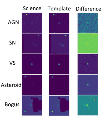
Figure 1: Examples of ZTF alerts of five classes of astronomical objects: AGN, SN, VS, Asteroid and Bogus.

result by its standard deviation. We split our data into train, validation and test sets, taking randomly 100 samples per class for the validation set and 100 samples per class for the test set.

3.2 Enhanced stamp classifier model

The random rotations procedure is described in what follows. The algorithm has three parameters. The first parameter is the number of rotations $k$, which are equally spaced, following the function $r=[360/k]°$ which rotates the images by $r$ degrees. The second parameter is the rotation range $\theta$, which defines how much an image can rotate around a fixed point. For instance, if $k=5$ and $\theta=10°$, then the first rotation will take any value in $72°\pm 10°$, as shown in Figure 3. This operation is carried out at each iteration of the model. Using this notation, the original stamp classifier is described by $k=4$ and $\theta=0°$.The convolutional neural network model receives a triad of images of $45\times 45$, which includes k-rotated versions of each alert image, resulting in an augmented batch $B(x)=[x,rx,...,r^{k-1}x,r^{k}x]$; and then, each rotated image is cropped at the center in $a\times a$, where $a$ is a search parameter. All the convolutional layers, except for the first and the last one, use zero padding in order to keep the same dimension at the output of each layer, and are followed by ReLU activation functions. The output of the last Max Pooling layer is flattened to form the vectors that enter the Fully Connected layer, as shown at the middle of Figure 3. This is the last layer that works independently with the different rotations. At the output of this Max Pooling layer, the vectors of each rotation are stacked, obtaining a $k\times 64$ tensor, and the values in the stacked dimension are averaged, finally obtaining a 64-dimensional vector, this process is called Cyclic Pooling. The metadata is concatenated at the output of the cyclic pooling, obtaining a vector of 87 dimensions, which is inputted to the Fully Connected layers, to obtain the estimated probabilities for the 5 classes. The enhanced stamp classifier is shown in Figure 3.

3.3 Experiments

We tested all the hyperparameter combinations shown in Table 1 with 5 initializations for every combination including a total rotation range $\theta=360°$. The latter means random rotations between $0°$ and $360°$, i.e., total random rotations without restrictions. We obtained the average accuracy in the validation set, and selected the top 5 results shown in Table 2. At the bottom of this table, we present the results of the baseline model $M_{b}$ and the model with fully random rotations $M_{r}$ for comparison purposes. Next, using the best hyperparameters, each model was trained 20 times to get a more robust result. Figure 2 shows the confusion matrix obtained with the original Stamp Classifier, and Figure 4 shows the confusion matrix obtained with the enhanced Stamp Classifier, which includes random rotations and a different image cropping.Table 2 shows that the best image sizes are between 27 and 39 pixels per side, achieving the best results with an image of $33\times 33$. Likewise, the best number of rotations and rotation range, are 4 or more rotations and a rotation range close to $0.1$ [rad]. This is corroborated by the p-value obtained comparing the proposed models with the baseline model, obtaining values smaller than $0.05$ for the top 5 models in the table. These p-values were obtained with 5 repetitions of the same experiments and using the permutation test [4]. In the case of fully random rotations ($\theta=360°$), i.e., the model $M_{r}$, the results were inconsistent between different tests. The results could go from a low accuracy ($91.3\%$) to a high accuracy ($93\%$) depending on the iteration that was made. For instance, the best model with $360°$ of rotation range (using 5 rotations and a image size of $33\times 33$) give us a good result the first time that we tested it, but when the process was repeated, the results varied. When the rotation range is $360°$, we obtain a totally different variation every time that the model is called, one call could give rotations equispaced and in another one rotations closer to each other.Figures 2 and 4 show robust statistical results when using 20 repetitions for each experiment. The difference between both experiments is statistically significant with a p-value of $0.01$. This led us to conclude that the inclusion of random rotations with a larger image crop size is a relevant improvement to the Stamp Classifier.

Hyperparameter	Search values
k rotations	4; 5; 6; 7; 8
Rotation range $\theta$	$0^{o}$; $7^{o}$; $14^{o}$, $22^{o}$; $29^{o}$; $36^{o}$; $360°$
$a$	21, 27, 33, 39

Table 1: Hyperparameter search for enhancing the original Stamp Classifier through random rotations.

Model	Hyperparameter	Test accuracy	p-value
$M_{1}$	$a:33$ ; $k:6$ ; $\theta:$ $0.08$	$93.36\pm 0.4$	$0.007$
$M_{2}$	$a:27$ ; $k:6$ ; $\theta:$ $0.1$	$92.96\pm 0.5$	$0.008$
$M_{3}$	$a:27$ ; $k:5$ ; $\theta:$ $0.1$	$92.84\pm 0.4$	$0.008$
$M_{4}$	$a:39$ ; $k:8$ ; $\theta:$ $0.08$	$92.84\pm 0.3$	$0.007$
$M_{5}$	$a:27$ ; $k:7$ ; $\theta:$ $0.08$	$92.72\pm 0.3$	$0.007$
$M_{r}$	$a:33$ ; $k:5$ ; $\theta:$ $1$	$92.22\pm 0.8$	$0.3$
$M_{b}$	$a:21$ ; $k:4$ ; $\theta:$ 0	$91.44\pm 0.4$	Reference

Table 2: Top-5 models with the highest validation accuracies obtained from the hyperparameter search, ranked from $M_{1}$ to $M_{5}$. $M_{r}$ stands for the best model for a fully random rotation. $M_{b}$ stands for the baseline Stamp Classifier.

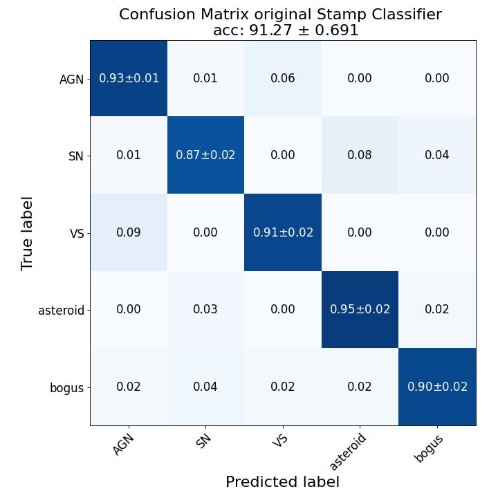
Figure 2: Confusion matrix of the original Stamp Classifier [1] using our own implementation.

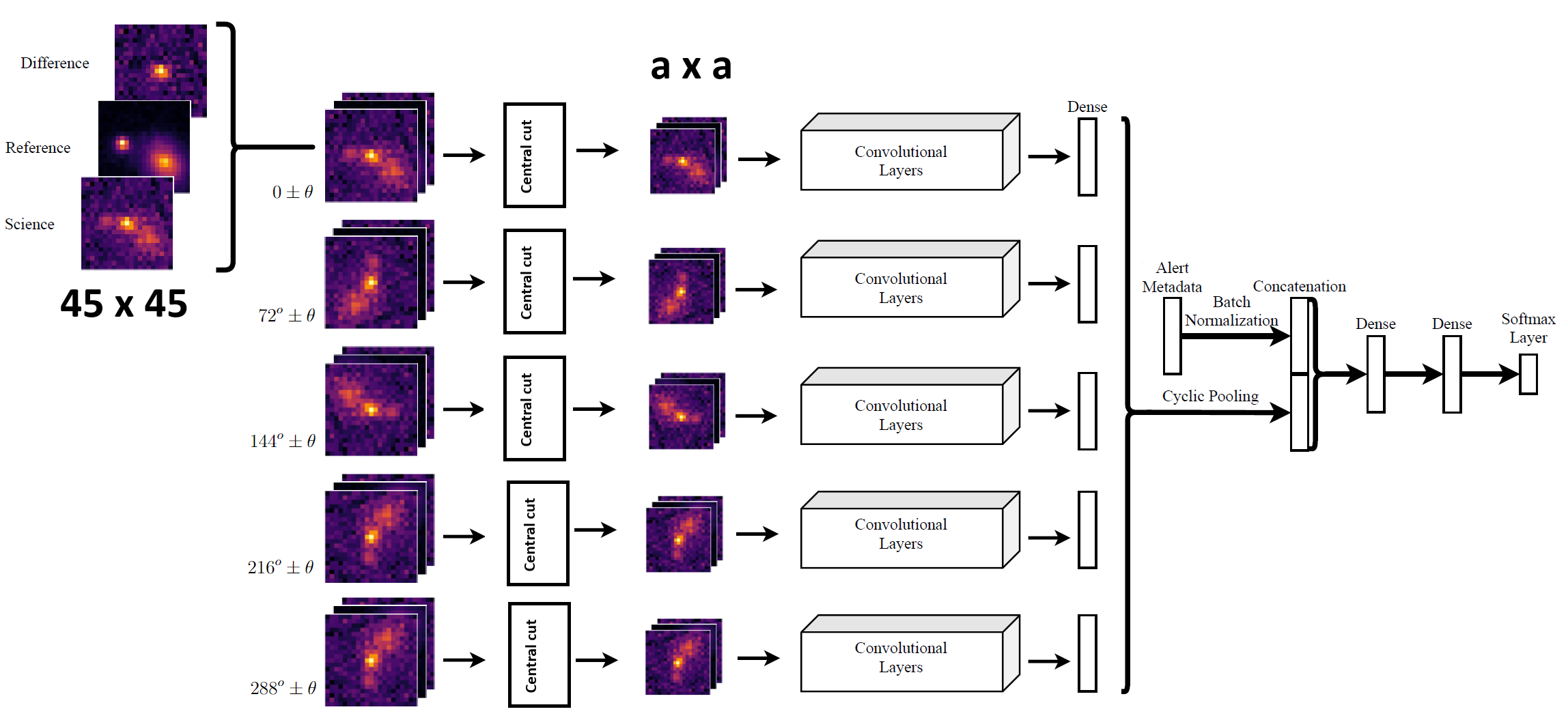
Figure 3: Enhanced Stamp Classifier model with $k=5$ rotations and a rotation range $\theta$.

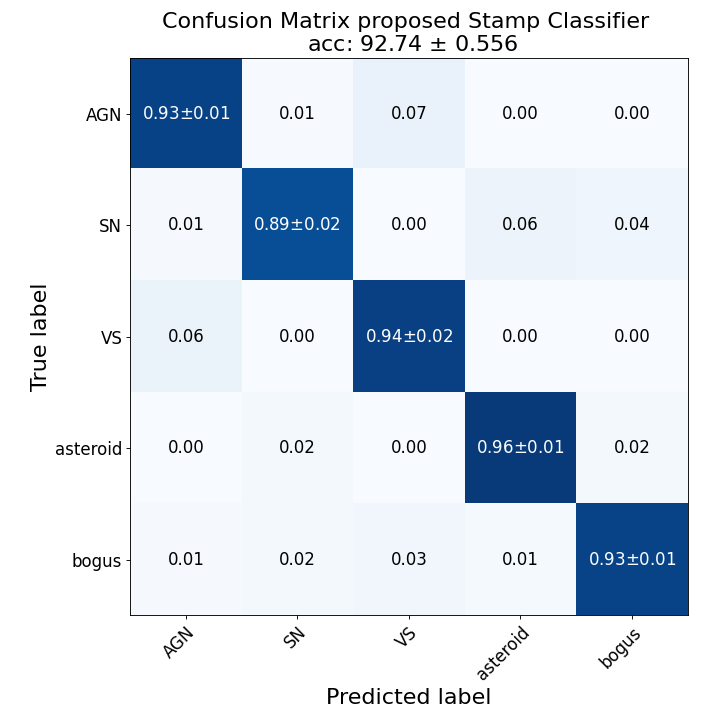
Figure 4: Confusion matrix of the enhanced Stamp Classifier that includes an image size of $33\times 33$ and 6 rotations with $0.08[rad]$ of rotation range.

4 Temporal Stamp Classifier: Extending the original model.

In this work, we use sequence of alerts reported by ZTF and classify them into three categories: AGN, SN and VS classes. We assume that alerts with more than one detection correspond only to real objects, so the bogus class can be discarded. In section B we discuss about how to detect bogus with more than one detection. In addition, as we are looking repeatedly at specific locations in the sky, asteroids can also be discarded because they are moving objects.Our aim is to use sequences of 2 to 5 alerts and improve the results obtained when using just the first detection and approach the results of the light curve classifier [2], which uses 6 or more detections. We use the information given by the images and the features, with the inclusion of crossmatch with the AllWISE catalog[5], as inputs to a neural network model that includes convolutional neural networks and recurrent neural networks. We compare the results obtained with different recurrent neural networks from the vanilla model to LSTM.

4.1 Data

The data used in this section was reported by the ZTF survey. It contains samples from objects detected once or more times. The data considers 4 classes of objects AGN, SN, VS, and bogus with a number of examples of $48262$ ($28.7\%$), $2524$ ($1.5\%$), $101038$ ($60.1\%$), and $16332$ ($9.7\%$), respectively, with a total of $168,156$ examples.Each sample contains 1 to 10 alerts of the objects. Each alert is composed of three images called stamps and metadata related to the source, the observation conditions of the exposure, and other useful information. The stamps are cropped at 63 pixels on a side from the original image and centered at the position of the object. The metadata used in this work is the same as in [1], except for the inclusion of AllWISE colors [5] information through crossmatch by positions in the sky.The dataset described above was pre-processed. First, all bogus examples were discarded. Alerts with images with a shape different from $63\times 63$ were discarded, because it is considered an error in capture. Then all consecutive alerts with less than 6 hours of difference between each other were discarded. In addition, all difference images were discarded, and the remaining images were cropped at $33$ pixels centered at the point of interest, and normalized between 0 and 1. For metadata used as features, we limit their values as shown in Table 3, using the training set, and then we normalize each feature by subtracting its mean value in the training set and dividing the result by its standard deviation. Each number of detections has its own limit value for each metadata. Additionally, we separated metadata according to its time variability into static metadata and dynamic metadata. For instance, the PSF-Magnitude is dynamic because it’s related with the magnitude of the flux measured in the given detection, while the Star Galaxy Score (sgscore) stands for star near the source that depends on the position of the object and this value shouldn’t change with the detections. The static/dynamic category of every metadata is shown in Table 3.

Metadata	[min value, max value]	Category
sgscore 1	[-1, max]	Static
distpsnr1	[-1, max]	Static
sgscore2	[-1, max]	Static
distpsnr2	[-1, max]	Static
sgscore3	[-1, max]	Static
distpsnr3	[-1, max]	Static
ifwhm	[min, 10]	Dynamic
ndethist	[min, 20]	Dynamic
ncovhist	[min, 3000]	Dynamic
chinr	[-1, 15]	Static
sharpnr	[-1, 1.5]	Static
no-detections	[min, 2000]	Dynamic
isdiffpos	[min, max]	Dynamic
magpsf	[min, max]	Dynamic
sigmapsf	[min, max]	Dynamic
RA, DEC	[min, max]	Static
diffmaglim	[min, max]	Dynamic
classtar	[min, max]	Dynamic
Galactic Coordinates	[min, max]	Static
Ecliptic Coordinates	[min, max]	Static

Table 3: Range of values for each metadata. Max and min stand for the maximum and minimum values obtained in the training set. The definition of the metadata can be found in [1].

4.2 Bogus with more than one detection

The dataset described above has $16,332$ bogus samples, and only $253$ of these samples has more than one detection. This is because most bogus, e.g. cosmic rays, don’t appear in the same position twice. In order to detect bogus with more than one detection, we propose to use the Enhanced Stamp Classifier model with the first and the second detection and, if the model predicts a sample as bogus in the first and second detection, it can be considered as bogus and discarded. We tested $253$ bogus with the enhanced stamp classifier model, obtaining an accuracy of $86\%$ for bogus samples in the first detection and $84\%$ in the second detection. This result indicates that a total of $32$ out of $16,332$ bogus samples could go undetected. Representing less than $0.2\%$ of bogus. This small number of cases does not allow to build a Deep Learning based classifier. This problem should be addressed directly using other approaches.

4.3 Temporal Stamp Classifier model

As mentioned above, the goal is to develop a deep learning-based model that processes a short sequence of alerts, i.e., where the number of detections is $n\in\{2,3,4,5\}$. The enhanced stamp classifier uses convolutional neural networks (CNNs) to process a triad of images and their rotations. In the proposed model, CNNs are the first step, as shown in Figure 5.The random rotations procedure is the same as the enhanced stamp classifier, with the addition of a third parameter that consists of the number of detections $n$.The convolutional neural network model receives a set of images for each detection, which includes k-rotated versions of each alert image, resulting in an augmented batch $B(x)=[x,rx,...,r^{k-1}x,r^{k}x]$; and generates an output for each detection. All the convolutional layers, except for the first and the last one, use zero padding in order to keep the same dimension at the output of each layer, and are followed by ReLU activation functions. The output of the last Max Pooling layer is flattened to form the vectors that enter the Fully Connected layers, as shown at the middle of figure 5. This is the last layer that works independently with the different rotations. At the output of this Max Pooling layer, the vectors of each rotation are stacked, obtaining a $k\times 64$ tensor, and the values in the stacked dimension are averaged, finally obtaining a 64-dimensional vector for each detection, this process is called Cyclic Pooling. The output of the n detections, a vector of size $n\times 64$, is concatenated with a vector of time differences among detections, plus the metadata, resulting in a vector of size $n\times 72$. This concatenated vector is the input of a recurrent neural network (RNN), obtaining a final output vector of 72 dimensions. After completing this recurrent processing, the static metadata is concatenated, obtaining a vector of 87 dimensions, which is inputted to the Fully Connected layers, to obtain the estimated probabilities for the 3 classes.As shown in Figure 5 and Table 4, the recurrent layer is not defined beforehand, allowing us to test several different recurrent models from vanilla RNN to LSTM.

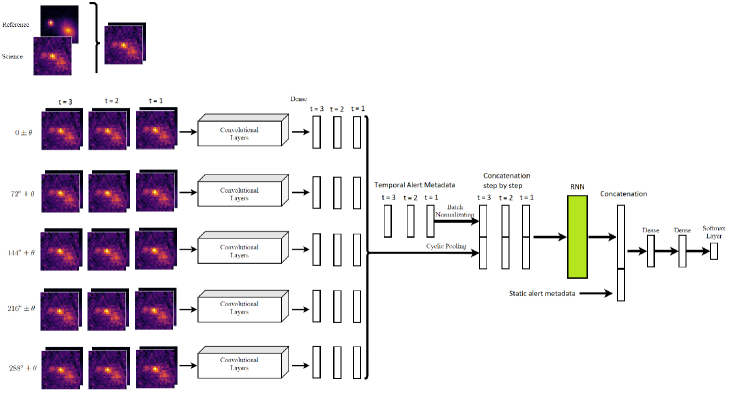
Figure 5: Temporal Stamp Classifier model with $k=5$ and a range of rotation $\theta$. Convolutional layers refers to the convolutional filters of table 4 from the first Convolution to Flatten layers. For each sample, we use science and template images as inputs and metadata that are separated into dynamic and static features.

4.4 Experiments

In this section, we first describe the experiments to select the best hyperparameters of our proposed model. Every experiment run was trained up to $30,000$ iterations, the loss was evaluated in the validation set every 10 iterations, and the best model so far was saved.

Layer	Parameters	Output size
Input	-	$t\times 33\times 33\times 3$
Rotation augmentation	-	$t\times 33\times 33\times 3$
Convolution	$4\times 4$, 32	$t\times 24\times 24\times 32$
Convolution	$5\times 5$, 32	$t\times 24\times 24\times 32$
Max pooling	$2\times 2$, stride 2	$t\times 12\times 12\times 32$
Convolution	$5\times 5$, 64	$t\times 12\times 12\times 64$
Convolution	$5\times 5$, 64	$t\times 12\times 12\times 64$
Convolution	$5\times 5$, 64	$t\times 12\times 12\times 64$
Max pooling	$2\times 2$, stride 2	$t\times 6\times 6\times 64$
Flatten	-	$t\times 2304$
Fully connected	$2304\times 64$	$t\times 64$
Rotation concatenation	-	$t\times 6\times 64$
Cyclic pooling	-	$t\times 64$
Concat with dynamic metadata after BN	-	$t\times 64+8$
RNN	Variable	$72$
Concat with static metadata after BN	-	$87$
Fully Connected with dropout	$90\times 64$	$64$
Fully connected	$64\times 64$	$64$
Fully Connected with softmax	$64\times 3$	$3$ (n° classes)

Table 4: Temporal Stamp Classifier architecture.

After the first $20000$ iterations, if a lower loss is obtained on the validation set, another $10000$ iterations are performed. The validation and testing sets are randomly sampled just once before starting any experiment, and these sets are kept the same for all experiments. $200$ samples per class are taken from the whole dataset, totaling $600$ samples for each of the two subsets validation, and testing; the rest of the samples were used for training. Every experiment was trained 10 times, and the average and standard deviation are reported. The Adam optimizer was used, with its default hyperparameters, a learning rate of 1e-4 and batch size of $128$. The training was performed in a $GTX1080Ti$ GPU.

4.4.1 Recurrent model

In order to determine the best temporal model for each number of alerts, we searched the hyperparameter values shown in table 5 for six models: LSTM [6], GRU [7], SimpleRNN, Gamma Memory [8], Convolution in one dimension (Conv1D) [9] and TDNN [10].To process the images, we used the configuration of the enhanced stamp classifier in Section III that consists of $k=6$ rotations with a range of rotation of $\theta=0.08[rad]$ and an image size $a=33$. The output of the convolutional layers was stacked with the time differences between alerts, forming the input to the recurrent layers. No metadata was used in this experiment. Next, the output of the recurrent layer was injected into an MLP with softmax activation to determine the class of each sample.Table 6 shows the best configuration obtained for each model for each number of alerts. We present the accuracy achieved in the test set and the p-value obtained between the proposed model and the LSTM model for each number of alerts, as well as the inference time (IT) for the model. LSTM was chosen as the baseline model for comparison purposes because it is the most complex model used in our experiments. In table 6, $A$ stands for the number of alerts, $L$ the number of layers, $U$ the number of units, $k$ the number of Leaky Filters, $V$ stands for time windows, and $Ke$ is the kernel size for the 1D convolution.The results show that there are no significant differences among the tested recurrent models in terms of accuracy, resulting in similar values for every number of alerts used in this work. This is ratified by the p-values of the permutation hypothesis test [4] obtained between the different models and LSTM. The p-values are bigger than 0.05 for every pairwise of models.On the other hand, the best configuration for most recurrent model tends to be the simplest one. A single layer in the case of layer-dependent models (LSTM, GRU and SimpleRNN), and a small kernel size for Conv1D. In contrast, Gamma Memory requires a substantial number of Leaky Filters. In terms of inference time (IT), the Gamma Memory and Conv1D tend to be 4 times faster in processing a sample for 2, 3 and 4 alerts, while the rest of the models have similar computational times for every configuration used. Figure 6 shows that the difference between inference times of these models is important, having Gamma Memory and Conv1D separated by a considerable distance from the others models, which are grouped together. This result is similar for all number of alerts as shown in Table 6. This difference in time inference is relevant for the use of the model in a production environment.As the number of alerts increased, the accuracy obtained by the models increased too, but not substantially. This may be due to the fact that the information given by stamp images is not enough to solve the problem and additional metadata is needed. These results confirm that simple recurrent models and even Conv1D are competitive with complex models such as LSTM and GRU for short sequences of data and are more effective since their inference time is shorter. In order to choose the best model, as the results are similar and has no statistically significant difference, we choose the model with the lower inference time, in order to use it later in a production environment.

Model	Cells	Layers
LSTM	32, 64, 128	1, 2, 3
GRU	32, 64, 128	1, 2, 3
SimpleRNN	32, 64, 128	1, 2, 3
Model	Filters k
Gamma Memory	1, 2, 3, 4, 5, 6, 7, 8
Model	Filter size
TDNN	2
Conv1D	2,…,A

Table 5: Hyperparameter search to determine the best model for processing short sequence of alerts. A represent the number of alerts and $k$ stands for the number of Leaky Filters for the Gamma Memory model.

	Model	GRU	LSTM	G. M.	TDNN	RNN	Conv1D
2 A	Acc.	$91.3\pm 0.4$	$91.7\pm 0.3$	$91.3\pm 0.2$	$91\pm 0.1$	$91.2\pm 0.7$	$91.3\pm 0.6$
	p-v.	$0.35$	Ref.	$0.1$	$0.1$	$0.68$	$0.3$
	Arc.	1L 256U	1L 256U	$k=7$	$V=2$	1L 128U	$Ke=2$
	IT	21.04	20.57	5.47	22.68	24.63	5.75
3 A	Acc.	$91.8\pm 0.4$	$92\pm 0.3$	$91.4\pm 0.5$	$91.6\pm 0.1$	$91.8\pm 0.4$	$91.6\pm 0.6$
	p-v.	$0.28$	Ref.	$0.06$	$0.07$	$0.08$	$0.1$
	Arc.	1L 256U	1L 64U	$K=7$	$V=2$	1L 128U	$Ke=3$
	IT	30.42	29.63	7.84	32.88	30.42	8.33
4 A	Acc.	$92.5\pm 0.4$	$92.2\pm 0.6$	$92.2\pm 0.5$	$92.4\pm 0.5$	$92.4\pm 0.4$	$92.5\pm 0.6$
	p-v.	$0.31$	Ref.	$0.81$	$0.68$	$0.69$	$0.48$
	Arc.	1L 256U	3L 256U	$K=6$	$V=2$	1L 64U	$Ke=2$
	IT	39.31	46.06	10.86	40.8	49.02	11.13
5 A	Acc.	$93.2\pm 0.5$	$92.9\pm 0.3$	$92.6\pm 0.4$	$92.9\pm 0.3$	$92.6\pm 0.6$	$93.2\pm 0.6$
	p-v.	$0.23$	Ref.	$0.24$	$0.98$	$0.2$	$0.29$
	Arc.	1L 64U	1L 128U	$k=8$	$V=2$	1L 64U	$Ke=4$
	IT	55	50.54	55.06	57.16	57.44	71.48

Table 6: Best results for each of the five recurrent models, plus Conv1D, tested per number of alerts ($\#A$). Here only images were used. For each model, we show the best configuration of hyperparameters (Arc), the average test accuracy and standard deviation of 10 iterations (Acc), the inference time (IT), and the p-value of each model against the LSTM model corresponding to the number of alerts.

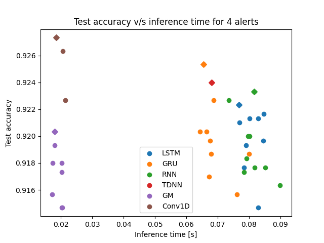
Figure 6: Test accuracy v/s inference time for 4 alerts. Diamonds represent the best configuration for a given model in terms of test accuracy.

4.4.2 Cross-matching detections with AllWISE catalog

In [2], it was shown that the information from the AllWISE catalog improves the classification of stochastic objects, being the most valuable information according to random forest importance values.In order to improve the discrimination between AGN and VS, we included information on the match radius of 2 arcseconds, obtaining W1, W2, W3, and W4 photometry, and calculating the difference between these magnitudes W1-W2, W2-W3, and W3-W4, which are used as new metadata. We trained a model using only metadata as input, where the features are separated into static and dynamic metadata, according to its temporal behavior. Dynamic metadata are injected in an LSTM layer, that processes the recurrent dependences present on the metadata. The output of the LSTM layer is concatenated with static metadata and then injected into MLP layers to obtain the final classification score.We trained models with AllWISE information and without it. The model use the static and dynamic metadata, and we consider AllWISE as a static metadata due to it’s dependence with the position of the object. Table 7 shows the average accuracy and standard deviation of 5 random initializations, obtained for each number of alerts with and without AllWISE information. In addition, the p-value between both models is given.The results of table 7 show that the crossmatch between the original dataset and the AllWISE catalog improves the performance of the proposed model for every number of alerts, achieving a $3\%$ increase in accuracy for the case of 2 alerts and $1.3\%$ for 5 alerts. This result is corroborated by the p-values obtained for 2, 3, and 4 alerts, being all smaller than $0.05$, meaning that the distributions of both models are different and have statistical significance. For 5 alerts, the p-value is 0.08, meaning that the improvement by the AllWISE catalog is not statistically significant in this case. This improvement in the accuracy of the model comes mostly from a better discrimination between AGN and VS. In [2], it is stated that AllWISE colors are essential to discriminate among AGN subclasses and to identify these kinds of objects from others. In the case of this work, the AllWISE information can be used with 2 or more alerts for real objects with a fixed position in the sky.

4.4.3 Complete model

The complete temporal stamp classifier model for the classification of sequences of astronomical alerts is a concatenation of the best models found in the previous experiments. Each number of detections has it’s own model trained separately. The complete model uses the best parameters found for the convolutional filters, followed by concatenation of the dynamic metadata, thus being processed by the best model for every number of detection found in Table 6 in terms of inference time and summarized in Table 8. The output of the recurrent layer is then concatenated with the static metadata including AllWISE catalog information obtained through crossmatch, then inputted to MLP layers with ReLU as their function activation except for the last layer, which have a softmax activation. The architecture of the proposed temporal stamp classifier is shown in Figure 5.

Model / Alerts	2 alerts	3 alerts	4 alerts	5 alerts
Without AllWISE	$95.07\pm 0.57$	$96.1\pm 0.32$	$96.9\pm 0.25$	$97.37\pm 0.55$
With AllWISE	$98\pm 0.56$	$98.27\pm 0.27$	$98.37\pm 0.29$	$98.07\pm 0.29$
p-value	$0.01$	$0.01$	$0.008$	$0.08$

Table 7: Results of recurrent models that use only metadata as input with and without AllWISE information for every number of alerts. The average accuracy and standard deviation of 5 iterations for each model, as well as the p-value between the model with and without AllWISE information, are shown.

Table 8 shows the test accuracy obtained with the best model for each number of alerts when using recurrent models or Conv1D in terms of inference time. We also present the confusion matrices for each number of alerts in Figure 7.The models shown in table 8 corresponds to the best configuration obtained in the previous experiments, and it’s dominated by Conv1D model for the case of 2, 3 and 4 detections, and by LSTM in 5 detections. The configuration for every model tends to be the simplest one and the accuracy obtained in test partition tends to be similar between the number of alerts except for 4 alerts. These results can be interpreted as the model reaching a limit in terms of its performance in the task at hand, which has as a consequence that there is no improvement in accuracy as we add more alerts to the model. An interesting option is to increase the number of classes, expanding in a controlled way some of the classes (SN for example) into their subclassifications like the light curve classifier. The decrease in accuracy for the 4 alerts model could be just a statistical coincidence because the model with less and more detections have better performances and the decrease it is just of $0.5\%$. These results are competitive with the ones obtained in [2], reaching a comparable value of accuracy with a different test set. The proposed temporal stamp classifier achieves more successful prediction than the original stamp classifier for the first detection for the classification of the three classes considered, filling the gap between the light curve model and the first detection model. See Figure 8.

4.4.4 Comparison with baseline models

In order to corroborate the effectiveness of the proposed model, we compare its performance with those of the ALeRCE models [1] and [2]. We took all the test samples and made calls to the ALeRCE API [11], obtaining the classification made by the stamp classifier and the light curve classifier, and comparing the results with the true class. In this way, we obtained the confusion matrices shown in Figures 8 and 9.The results of the original Stamp Classifier [1] show that it can predict relatively well the SN and AGN classes, but the class VS is confused with AGN in $12\%$ of the cases. This difficulty is mainly solved in our model by including the crossmatch with the AllWISE catalog. Notice that the original stamp classifier deals with 5 classes instead of 3, because it includes asteroids and bogus that maybe present in a single detection. In the case of the Light Curve Classifier [2], Figure 9 shows that the predictions with our test samples are pretty similar to our own results, shown in Figure 7 for different numbers of alerts. These results show that the proposed temporal stamp classifier is able to fill the gap between the two ALeRCE models currently in production. This allows improving the confidence in the classification when the object is detected more than one time, and merge the information given by the images with the metadata.

	Model	Architecture	Test accuracy
2 alerts	Conv1D	$Ke=2$	$98.47\pm 0.1$
3 alerts	Conv1D	$Ke=3$	$98.33\pm 0.7$
4 alerts	Conv1D	$Ke=2$	$97.87\pm 0.2$
5 alerts	LSTM	1L 128U	$98.43\pm 0.3$

Table 8: Best model configuration by inference time obtained by number of alerts, according to Table 6. Test accuracy stands for the accuracy of the complete model that uses images and metadata. Ke stands for Kernel size, L the number of layers and U stands for Units.

a 2 alerts

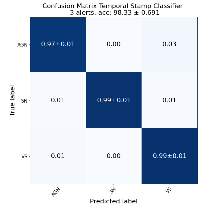
b 3 alerts

c 4 alerts

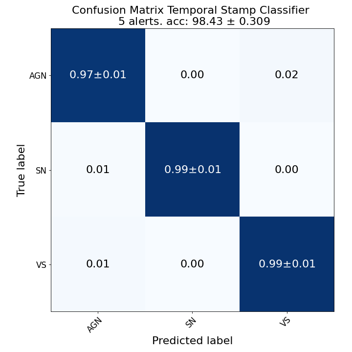
d 5 alerts

Figure 7: Average confusion matrix for the test set using 5 different realizations of the temporal stamp classifier for each number of alerts using the model configurations of Table 6.

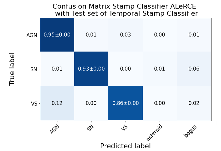
Figure 8: Confusion matrix of original Stamp Classifier [1] in the test set.

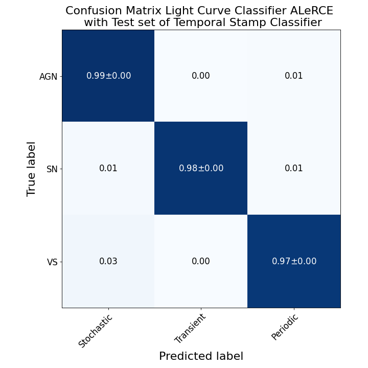
Figure 9: Confusion matrix of Light Curve Classifier [2] in the test set.

5 Conclusions

The proposed temporal stamp classifier is a significant improvement for the early classification of astronomical events, allowing us to go beyond the prediction of the first alert of an astronomical event using sequences of images from the alerts, the time information, metadata, and crossmatch with the AllWISE catalog. In addition, we proposed an enhanced stamp classifier for a single detection, by adding random rotations and changing the size of the stamps (cropped images). This led to a statistically significant increase in the performance of the stamp classifier.As future work, we propose to split the current three classes into known subgroups in order to take advantage of the extra information given by a larger number of alerts. For instance, we can split the SN class into SN type Ia and all other types of SN. Another idea comes from [12], where the time is modulated by a function, which allows improving the results in the classification of SNe, in contrast with using the time difference between detections. The proposed temporal stamp classifier might be used to find outliers like [13, 14], e.g., using the model uncertainty operator proposed in [15] to find examples that are in the tail of the distributions. Finally, deep attention models (transformers) could be used instead of recurrent models or to process images directly [16, 17].

References

- [1] R. Carrasco-Davis et al., “Alert classification for the alerce broker system: The real-time stamp classifier,” The Astronomical Journal, vol. 162, p. 231, nov 2021.
- [2] P. Sánchez-Sáez et al., “Alert Classification for the ALeRCE Broker System: The Light Curve Classifier,” The Astronomical Journal, vol. 161, p. 141, Mar. 2021.
- [3] F. J. Masci et al., “The zwicky transient facility: Data processing, products, and archive,” Publications of the Astronomical Society of the Pacific, vol. 131, p. 018003, dec 2018.
- [4] E. J. G. Pitman, “Significance tests which may be applied to samples from any populations,” Supplement to the Journal of the Royal Statistical Society, vol. 4, no. 1, pp. 119–130, 1937.
- [5] E. L. Wright et al., “The Wide-field Infrared Survey Explorer (WISE): Mission Description and Initial On-orbit Performance,” The Astronomical Journal, vol. 140, pp. 1868–1881, Dec. 2010.
- [6] S. Hochreiter et al., “Long short-term memory,” Neural computation, vol. 9, pp. 1735–80, dec 1997.
- [7] K. Cho et al., “Learning phrase representations using RNN encoder–decoder for statistical machine translation,” in Proceedings of the 2014 Conference on Empirical Methods in Natural Language Processing (EMNLP) (A. Moschitti, B. Pang, and W. Daelemans, eds.), (Doha, Qatar), pp. 1724–1734, Association for Computational Linguistics, Oct. 2014.
- [8] B. de Vries et al., “The gamma model—a new neural model for temporal processing,” Neural Networks, vol. 5, no. 4, pp. 565–576, 1992.
- [9] K. Fukushima, “Neocognitron: A self-organizing neural network model for a mechanism of pattern recognition unaffected by shift in position,” Biological Cybernetics, vol. 36, pp. 193–202, 1980.
- [10] A. Waibel et al., “Phoneme recognition using time-delay neural networks,” IEEE Transactions on Acoustics, Speech, and Signal Processing, vol. 37, no. 3, pp. 328–339, 1989.
- [11] ALeRCE, “Alerce client,” 2020. API ALeRCE documentation, https://alerce.readthedocs.io/en/latest/.
- [12] O. Pimentel et al., “Deep attention-based supernovae classification of multiband light curves,” The Astronomical Journal, vol. 165, p. 18, jan 2023.
- [13] M. Perez-Carrasco et al., “Alert classification for the alerce broker system: The anomaly detector,” The Astronomical Journal, vol. 166, p. 151, sep 2023.
- [14] P. Sánchez-Sáez et al., “Searching for changing-state agns in massive data sets. i. applying deep learning and anomaly-detection techniques to find agns with anomalous variability behaviors,” The Astronomical Journal, vol. 162, p. 206, oct 2021.
- [15] R. Singh et al., “A Physics inspired Functional Operator for Model Uncertainty Quantification in the RKHS,” arXiv e-prints, p. arXiv:2109.10888, Sept. 2021.
- [16] A. Dosovitskiy et al., “An image is worth 16x16 words: Transformers for image recognition at scale,” in 9th International Conference on Learning Representations, ICLR, OpenReview.net, 2021.
- [17] A. Vaswani et al., “Attention is all you need,” in Advances in Neural Information Processing Systems (I. Guyon, U. V. Luxburg, S. Bengio, H. Wallach, R. Fergus, S. Vishwanathan, and R. Garnett, eds.), vol. 30, Curran Associates, Inc., 2017.