Preferential Latent Space Models for Networks with Textual Edges

Abstract

Many real-world networks contain rich textual information in the edges, such as email networks where an edge between two nodes is an email exchange. Other examples include co-author networks and social media networks. The useful textual information carried in the edges is often discarded in most network analyses, resulting in an incomplete view of the relationships between nodes. In this work, we propose to represent the text document between each pair of nodes as a vector counting the appearances of keywords extracted from the corpus, and introduce a new and flexible preferential latent space network model that can offer direct insights on how contents of the textual exchanges modulate the relationships between nodes. We establish identifiability conditions for the proposed model and tackle model estimation with a computationally efficient projected gradient descent algorithm. We further derive the non-asymptotic error bound of the estimator from each step of the algorithm. The efficacy of our proposed method is demonstrated through simulations and an analysis of the Enron email network.

Keywords: latent space model; non-convex optimization; sparsity; text analysis; visualization.

1 Introduction

Over the past decades, the study of networks has attracted enormous attention, as they provide a natural characterization of complex systems emerging from a wide range of research communities, such as social sciences (Borgatti et al., 2009), business (Elliott et al., 2014) and biomedical research (Bota et al., 2003). In response to the rising needs in analyzing network data, many statistical network models have been developed, including the exponential random graph model (Frank and Strauss, 1986; Zhang and Chen, 2015), the stochastic block model (Wang and Wong, 1987; Nowicki and Snijders, 2001; Zhang et al., 2020a), the random dot product model (Athreya et al., 2018), the latent space model (Hoff et al., 2002; Ma et al., 2020; MacDonald et al., 2022), among others.

The majority of statistical research to date has focused on networks with binary (or weighted) edges that characterize the presence (or strength) of connections between nodes. Meanwhile, networks with textual edges, where an edge between two nodes is a text document, are fast emerging. Examples include email networks, where an edge between two nodes (i.e., email accounts) is an email, Twitter networks, where an edge between two nodes (i.e., Twitter accounts) is a comment or retweet, and coauthor networks, where an edge between two nodes (i.e., authors) is a paper. A common approach to analyze such networks is to discard the textual data and use binary or non-negative integer edges to encode the presence or frequency of exchanges. However, this simplified treatment may lose important information encoded in the text data and offer only an incomplete view of the interactions between nodes in the network. For instance, in email networks, discarding the text data carried in edges can overlook important context information in the email exchanges, and is unable to provide insights on the topics communicated in the emails or the sender/receiver preferences of these topics. To gain a more accurate and comprehensive understanding of the relationships between nodes, a more favorable approach is to incorporate the textual information when modeling the formation of network edges.

To extract textual information, useful representation tools from the natural language processing literature can be used. In particular, these tools aim to convert text documents to numerical vectors, which can then be used in text analysis. Some examples include Bag-of-Words that represents tokenized documents as sparse vectors of word counts (Joachims, 1998), embedding methods such as Word2Vec (Mikolov et al., 2013) and BERT (Devlin et al., 2018), that represent words as dense vectors. These word embedding vectors can capture, for example, semantic similarities and are pre-trained on very large text corpora using neural network models. The appropriate choice of representation tools often depends on the goal of analysis. For example, Word2Vec is useful for learning relationships between words and BERT is useful for translation and next-word prediction (Ke et al., 2023). It is worth noting that embedding methods like Word2Vec or BERT may lack interpretability, as it is unclear what each dimension in the embedding space represents, making the vector representations difficult to interpret.

In this paper, our goal is to model the relationships between nodes and understand how these relationships are modulated by the contents of textual exchanges. To effectively summarize contents, we represent each text document between a pair of nodes (i.e., textual edge) as a $K$-variate vector that counts the appearances of $K$ keywords in this document. The $K$ keywords are extracted from all text documents using techniques such as textRank (Mihalcea and Tarau, 2004) or topic modeling (Ke et al., 2023). This representation approach facilitates model interpretability and it converts a text document between nodes $i,j$ to a multivariate edge of dimension $K$, denoted as ${\bm{y}}_{ijl}=(y_{ijl}^{(1)},\ldots,y_{ijl}^{(K)})$, where $y_{ijl}^{(k)}$ counts the appearance of keyword $k$ in document $l$ between nodes $i,j$. In this paper, we refer to each edge dimension as a layer, although the network we analyze differs from a typical multi-layer network. In particular, one unique aspect of our data is that the number of nonzero multivariate edges between nodes may vary. For example, nodes $i,j$ may have 2 emails between them while nodes $i^{\prime},j^{\prime}$ have 20. As such, if each email is treated as a separate observation of edges between nodes, our data cannot be conveniently formulated into a multi-layer network as the number of nonzero edges observed between nodes can vary.

To model this network with multivariate edges, we propose a new preferential latent space framework that models edge probabilities as a function of latent node positions and node-layer preferences represented via parameter ${\bm{W}}\in\mathbb{R}^{n\times K}$, where $n$ is the number of nodes in the network and $W_{ik}$ characterizes the interest level of node $i$ on layer $k$. This flexible model gives direct insights on how contents of the textual exchanges modulate the relationships between nodes. As the number of keywords $K$ can be large, we further impose a sparsity assumption on ${\bm{W}}$ to improve model estimability and interpretability. We tackle model estimation with a computationally efficient projected gradient descent algorithm and theoretically derive the error bound of the estimator from each step of the algorithm.

Some recent works have considered modeling networks with edges that contain textual information. For example, Zhou et al. (2006); Sachan et al. (2012); Bouveyron et al. (2018); Corneli et al. (2019); Boutin et al. (2023) considered Bayesian community-topic models that extended the Latent Dirichlet Allocation (LDA) model to incorporate network communities. These works assume nodes in the network form several communities and the focus is to identify the community label of each node. Model estimation in these works is often carried out via Gibbs sampling or variational EM, which may be prohibitive when applied to large networks. In comparison, our goal is to understand the relationships between nodes and we do not impose assumptions on the community structure amongst nodes. There is another closely related line of research on modeling multi-layer networks. Multi-layer networks are special cases of the networks with multivariate edges we study, by allowing only one nonzero multivariate edge between two nodes. From our data, standard multi-layer networks can be constructed by merging the text documents between a pair of nodes into one. In this case, the edge between nodes $i,j$ on layer $k$ counts the appearance of keyword $k$ in all of the text documents between nodes $i,j$. For multi-layer networks, Paul and Chen (2020); Lei et al. (2020); Jing et al. (2021); Lei and Lin (2023); Lyu et al. (2023) and others considered community detection, and Gollini and Murphy (2016); Salter-Townshend and McCormick (2017); D’Angelo et al. (2019) studied Bayesian latent space models. Recently, Athreya et al. (2018); Zhang et al. (2020b) considered random dot product and latent space models for multi-layer networks that assume common latent node positions and layer-specific scaling matrices. However, the layer-specific scaling matrix scales all latent node positions equally and is unable to capture the varying level of interests from nodes on a specific layer. MacDonald et al. (2022) proposed a novel latent space model where the latent node positions are concatenations of common position coordinates and layer-specific position coordinates. This model may not work well when there is a large number of sparse layers as it is challenging to estimate the layer-specific positions in this case. We compare with both Zhang et al. (2020b) and MacDonald et al. (2022) in simulations and real data analysis. In particular, we find that our proposed method enjoys better prediction accuracy in the analysis of a real email network.

In summary, our work contributes to both methodology and theory. As to methodology, we propose a flexible preferential latent space model for networks with multivariate edges. The proposed model is able to effectively borrow information across a large number of sparse layers when estimating the latent node positions and also provide direct insights into the preferences of nodes on different layers. With respect to theory, we establish an explicit error bound for the projected gradient descent iterations that shows an interesting interplay between computational and statistical errors. Specifically, it demonstrates that as the number of iterations increases, the computational error of the estimates converges geometrically to a neighborhood that is within statistical precision of the unknown true parameter. The theoretical analysis is nontrivial, as it involves a new and tight concentration result that can handle varying numbers of edges between nodes, alternating gradient descent, orthogonal transformation, identifiability constraints, sparsity, and the non-quadratic form of the loss function.

The rest of our paper is organized as follows. Section 2 introduces the preferential latent space model for networks with multivariate edges and Section 3 discusses model estimation. Section 4 investigates theoretical properties of the estimator from our proposed algorithm. Section 5 reports the simulation results, and Section 6 conducts an analysis of the Enron email corpus data. The paper is concluded with a short discussion section.

2 Model

2.1 Notation

We start with some notation. Let $[k]=\{1,2\dots,k\}$. Given a vector ${\bm{x}}=(x_{1},\ldots,x_{d})^{\top}\in\mathbb{R}^{d}$, we use $\|{\bm{x}}\|_{0}$, $\|{\bm{x}}\|_{2}$ and $\|{\bm{x}}\|_{\infty}$ to denote the vector $\ell_{0}$, $\ell_{2}$ and $\ell_{\infty}$ norms, respectively. Write $\langle\bm{a},\bm{b}\rangle=\sum_{i}a_{i}b_{i}$ for $\bm{a},\bm{b}\in\mathbb{R}^{n}$. For a matrix ${\bm{X}}\in\mathbb{R}^{d_{1}\times d_{2}}$, we use ${\bm{X}}_{i.}$ and ${\bm{X}}_{.j}$ to denote the $i$-th row and $j$-th column of ${\bm{X}}$, respectively, and $X_{ij}$ to denote the $(i,j)$-th entry of ${\bm{X}}$. Moreover, let $\|{\bm{X}}\|_{F}$ and $\|{\bm{X}}\|_{op}$ denote the Frobenius norm and operator norm of ${\bm{X}}$, respectively, and $\|{\bm{X}}\|_{0}=\sum_{ij}1(X_{ij}\neq 0)$ denote the number of nonzero entries in ${\bm{X}}$. We use $\text{Diag}(x_{1},\ldots,x_{d})$ to denote a $d\times d$ diagonal matrix with diagonal elements $x_{1},\ldots,x_{d}$, and use $\circ$ to denote the Hadamard product. For two positive sequences $a_{n}$ and $b_{n}$, write $a_{n}\precsim b_{n}$ or $a_{n}=\mathcal{O}(b_{n})$ if there exist $c>0$ and $N>0$ such that $a_{n}<cb_{n}$ for all $n>N$, and $a_{n}=o(b_{n})$ if $a_{n}/b_{n}\rightarrow 0$ as $n\rightarrow\infty$; write $a_{n}\asymp b_{n}$ if $a_{n}\precsim b_{n}$ and $b_{n}\precsim a_{n}$.

2.2 Preferential latent space model

Suppose there are $n$ nodes in the network, and between nodes $i,j$, there are $m_{ij}$ document exchanges denoted as $\{{\bm{z}}_{ijl}\}_{l\in[m_{ij}]}$. Each ${\bm{z}}_{ijl}$ is a tokenized document consisting of a list of words. From the corpus $\{{\bm{z}}_{ijl}\}_{i,j\in[n],\,l\in[m_{ij}]}$, we extract a set of $K$ keywords. These keywords can be defined in several ways: as words with high co-occurrence frequencies with other words in the corpus, using the textRank algorithm (Mihalcea and Tarau, 2004); as words that represent latent topics within the corpus, using topic modeling techniques (Ke et al., 2023); or as pre-defined terms based on the specific goals of the analysis. Correspondingly, each document ${\bm{z}}_{ijl}$ can be represented as a $K$-dimensional vector ${\bm{y}}_{ijl}=(y_{ijl}^{(1)},\ldots,y_{ijl}^{(K)})$, where $y_{ijl}^{(k)}$ characterizes the appearance of keyword $k$ in document ${\bm{z}}_{ijl}$. In this work, we refer to $y_{ijl}^{(k)}$ as an edge when there is no ambiguity and ${\bm{y}}_{ijl}$ as a multivariate edge. To ease exposition, we focus on undirected binary-valued edges, that is, $y_{ijl}^{(k)}=y_{jil}^{(k)}\in[0,1]$, although our methods and results generalize directly to directed edges and other types of edge values (e.g., continuous, non-negative integers) using tools in generalized linear models. In summary, the network data we model can be denoted as $\mathcal{Y}=\{{\bm{Y}}_{ij}\}_{i,j\in[n]}$, where ${\bm{Y}}_{ij}\in[0,1]^{m_{ij}\times K}$ collects the $m_{ij}$ multivariate edges between nodes $(i,j)$, and the $l$th row of ${\bm{Y}}_{ij}$ is a length-$K$ vector ${\bm{y}}_{ijl}$. If there is no exchange between nodes $i$ and $j$, we define ${\bm{Y}}_{ij}=(0,\ldots,0)\in[0,1]^{K}$. In real applications, the number of layers $K$ can be large and edges in each layer, i.e., $\{y^{(k)}_{ijl}\}_{i,j\in[n],l\in[m_{ij}]}$, are often highly sparse.

We adopt a conditional independence approach (Hoff et al., 2002) which assumes each node $i$ has a unique latent position ${\bm{u}}_{i}\in\mathbb{R}^{d}$ and the model admits

$$\mathbb{P}(\mathcal{Y}\mid{\bm{U}},{\bm{\theta}})=\prod_{i\neq j,l,k}\mathbb{P}(y^{(k)}_{ijl}\mid{\bm{u}}_{i},{\bm{u}}_{j},{\bm{\theta}}),$$

where ${\bm{U}}=[\bm{u}_{1},\ldots,\bm{u}_{n}]^{\top}$ and ${\bm{\theta}}$ are the latent positions and other model parameters to be estimated. Given ${\bm{U}}$ and ${\bm{\theta}}$, we assume that $y^{(k)}_{ijl}$ follows a Bernoulli distribution, with $\Theta^{(k)}_{ij}=\text{log odds}(y^{(k)}_{ijl}=1\mid{\bm{U}},{\bm{\theta}})$ and

$$\Theta^{(k)}_{ij}=a_{i}+a_{j}+(W_{ik}\bm{u}_{i}^{\top})(W_{jk}\bm{u}_{j}),$$ (1)

where $a_{i}\in\mathbb{R}$ represents the node-specific baseline effect and $W_{ik}\geq 0$ is a weight parameter that quantifies the interest level of node $i$ in layer $k$. In particular, a larger $W_{ik}$ indicates a greater interest of node $i$ in layer $k$. If either node $i$ or $j$ is uninterested in layer $k$, meaning $W_{ik}=0$ or $W_{jk}=0$, then the log odds of $y^{(k)}_{ijl}=1$ reduces to the baseline level $a_{i}+a_{j}$. The parameters ${\bm{u}}_{i}$ and ${\bm{u}}_{j}$ are latent node positions, and the angle between them determines the likelihood of edges between nodes $i$ and $j$. When ${\bm{u}}_{i}$ and ${\bm{u}}_{j}$ point in the same direction, i.e., ${\bm{u}}_{i}^{\top}{\bm{u}}_{j}>0$, the two nodes are more likely to have an edge in any layer $k$. Additionally, if both nodes $i$ and $j$ have strong interests in layer $k$, meaning large $W_{ik}$ and $W_{jk}$, the likelihood of an edge between nodes $i$ and $j$ in layer $k$ is further increased.

We refer to model (1) as the preferential latent space model (PLSM) and discuss model identifiability conditions in Section 2.3. In this model, the probability of an edge between nodes $i,j$ in layer $k$ is determined by $W_{ik}W_{jk}{\bm{u}}_{i}^{\top}{\bm{u}}_{j}$. The multiplied weight $W_{ik}W_{jk}$ varies across node pairs and layers, allowing the model to flexibly account for varying interest levels from nodes on layers. The node-specific effect ${\bm{a}}=\left(a_{1},\ldots,a_{n}\right)^{\top}$ and latent positions in ${\bm{U}}$ are shared across the $K$ layers, enabling model (1) to effectively borrow information across a large number of sparse layers when estimating these parameters.

When $K$ is large, we impose element-wise sparsity on ${\bm{W}}$ to ensure its estimability. This stipulates that each node prefers only a subset of the $K$ layers, or equivalently, each layer is only preferred by only a subset of the nodes. This plausible assumption effectively reduces the number of parameters in the weight matrix ${\bm{W}}$ and enhances model interpretability.

2.3 Identifiability

Recall that ${\bm{a}}=\left(a_{1},\ldots,a_{n}\right)^{\top}\in\mathbb{R}^{n}$, $\bm{W}=\left(W_{ik}\right)_{i\in[n],k\in[K]}\in\mathbb{R}^{n\times K}$, ${\bm{U}}=[\bm{u}_{1},\ldots,\bm{u}_{n}]^{\top}\in\mathbb{R}^{n\times d}$. The following proposition states a sufficient condition for the identifiability of model (1), and its proof is collected in the supplement.

Proposition 1 (Identifiability)

Suppose two sets of parameters $\left({\bm{a}},{\bm{W}},{\bm{U}}\right)$ and $\left({\bm{a}}^{\dagger},{{\bm{W}}}^{\dagger},{\bm{U}}^{\dagger}\right)$ satisfy the following conditions:
(1) $\|\bm{u}_{i}\|_{2}=1$, $\|{\bm{u}_{i}^{\dagger}}\|_{2}=1$ for $i\in[n]$.
(2) ${\bm{W}}_{i^{\prime}k^{\prime}}=0$, ${{\bm{W}}_{i^{\prime}k^{\prime}}^{\dagger}}=0$ for some $i^{\prime}\in[n]$, $k^{\prime}\in[K]$.
Then, if the following holds for $i,j\in[n],k\in[K]$,

$$a_{i}+a_{j}+(W_{ik}\bm{u}_{i}^{\top})(W_{jk}\bm{u}_{j})=a_{i}^{\dagger}+a_{j}^{\dagger}+(W_{ik}^{\dagger}\bm{u}_{i}^{\dagger}{}^{\top})(W_{jk}^{\dagger}\bm{u}_{j}^{\dagger}),$$

there exists an orthonormal matrix ${\bm{R}}\in\mathbb{R}^{d\times d}$ satisfying ${\bm{R}}^{\top}{\bm{R}}={\bm{R}}{\bm{R}}^{\top}={\bm{I}}_{d}$, such that

$$\bm{a}^{\dagger}=\bm{a},\,\,{\bm{W}}^{\dagger}=\bm{W},\,\,{\bm{U}}^{\dagger}={\bm{U}}{\bm{R}}.$$

Condition (1) in the above proposition is a norm constraint, imposed to ensure ${\bm{W}}$ and ${\bm{U}}$ are identifiable. This condition confines all latent node positions to the unit sphere. Condition (2) assumes at least one entry in ${\bm{W}}$ is zero and this is imposed to ensure ${\bm{W}}$ and ${\bm{a}}$ are identifiable.

3 Estimation

Given network data $\mathcal{Y}=\{{\bm{Y}}_{ij}\}_{i,j\in[n]}$, where ${\bm{Y}}_{ij}\in[0,1]^{m_{ij}\times K}$, we aim to estimate ${\bm{a}}$, ${\bm{W}}$, ${\bm{U}}$. Under model (1), the negative log-likelihood function, up to a constant, can be written as

$$\ell\left(\bm{a},\bm{W},{\bm{U}}\right)=-\sum_{k=1}^{K}\sum_{i<j}^{n}\sum_{l=1}^{m_{ij}}\frac{1}{m_{ij}}\left\{y^{(k)}_{ijl}\Theta^{(k)}_{ij}+\log\left(1-\psi\left(\Theta^{(k)}_{ij}\right)\right)\right\},$$ (2)

where $\psi(x)=1/(1+\exp(-x))$. We consider the following optimization problem,

$$\min_{{\bm{a}}\in\mathbb{R}^{n},\bm{W}\in\mathbb{R}^{n\times K}_{+},{\bm{U}}\in\mathbb{R}^{n\times d}}\ell(\bm{a},\bm{W},{\bm{U}})\text{, \quad subject to }\|{\bm{W}}\|_{0}\leq s,$$ (3)

where $s$ is a tuning parameter that controls the sparsity of ${\bm{W}}$. To enforce sparsity and the positivity constraint on ${\bm{W}}$ along the solution path, we employ a truncation operator Truncate(${\bm{W}},s$) defined as,

$$[\operatorname{Truncate}({\bm{W}},s)]_{ik}=\begin{cases}W_{ik},&\text{ if }(i,k)\in\text{Supp}^{+}({\bm{W}},s),\\ 0,&\text{ otherwise, }\end{cases}$$

for ${\bm{W}}\in\mathbb{R}^{n\times K}$ and $s\leq nK$. The set $\text{Supp}^{+}({\bm{W}},s)$ denotes the $s$ entries in ${\bm{W}}$ with the largest values. To solve (3), we develop a projected gradient descent algorithm that is easy to implement and computationally efficient. Our estimation procedure is summarized in Algorithm 1.

Algorithm 1 Projected Gradient Descent Algorithm

  Input: network data $\mathcal{Y}$, initial values ${\bm{a}}^{(0)},\bm{W}^{(0)},{\bm{U}}^{(0)}$, step sizes $\eta_{{\bm{a}}},\eta_{{\bm{W}}},\eta_{{\bm{U}}}$.

  repeat for $t=0,1,\ldots,$     ${\bm{a}}^{(t+1)}={\bm{a}}^{(t)}-\eta_{{\bm{a}}}\nabla_{{\bm{a}}}\ell({\bm{a}},{{\bm{W}}}^{(t)},{\bm{U}}^{(t)})|_{{\bm{a}}={\bm{a}}^{(t)}}$;     ${{\bm{W}}}^{(t+1)}={\rm Truncate}\left[{\bm{W}}^{(t)}-\eta_{{\bm{W}}}\nabla_{{\bm{W}}}\ell({\bm{a}}^{(t)},{\bm{W}},{\bm{U}}^{(t)})|_{{\bm{W}}={\bm{W}}^{(t)}},s\right]$;     ${{\bm{U}}}^{(t+1)}={\bm{U}}^{(t)}-\eta_{{\bm{U}}}\nabla_{{\bm{U}}}\ell({\bm{a}}^{(t)},{{\bm{W}}}^{(t)},{\bm{U}})|_{{\bm{U}}={\bm{U}}^{(t)}}$; normalize rows of ${{\bm{U}}}^{(t+1)}$;

  until the objective function converges.

The parameters $\eta_{{\bm{a}}},\eta_{{\bm{W}}},\eta_{{\bm{U}}}$ control the step sizes in the gradient descent algorithm. Theorem 1 provides theoretical conditions on $\eta_{{\bm{a}}},\eta_{{\bm{W}}},\eta_{{\bm{U}}}$ to ensure the algorithm achieves a linear convergence rate. Based on these conditions, we discuss practical choices for these parameters. In practice, backtracking line search can be implemented for $\eta_{{\bm{a}}},\eta_{{\bm{W}}},\eta_{{\bm{U}}}$ at each step of the iteration to achieve fast convergence.

For the initialization of Algorithm 1, we consider a singular value thresholding based approach (Ma et al., 2020), which has demonstrated good empirical performance. See Section S1 in the supplement for details. The latent dimension $d$ and the sparsity $s$ are two tuning parameters in the proposed model. We select these two parameters using edge cross-validation (Li et al., 2020). Specifically, we divide all indices $\{i,j,l,k\}$’s into $L$ folds and use each fold as a validation set while training the model on the remaining $L-1$ folds. To calculate the cross-validation error on the validation set, we calculate the binomial deviance, and the $d$ and $s$ combination with the smallest cross-validation error is selected.

4 Theoretical Results

We define the parameter space as

$$\mathcal{F}_{n,d,k}(M_{1})=\bigg{\{}({\bm{a}},{\bm{W}},{\bm{U}})\bigg{|} \,\,\|{\bm{a}}\|_{\infty}\leq\frac{M_{1}}{4},\,\,\max_{i}\sum_{k}(W_{ik})^{2}\leq\frac{M_{1}}{2},\,\,\|{\bm{W}}\|_{0}<nk,$$ (4)

$$\|\bm{u}_{i}\|_{2}=1,\,\,\max_{i\neq j,k}\Theta_{ij}^{(k)}\leq-(1-C)M_{1}\bigg{\}},$$

where $M_{1}\geq 0$ is a scalar that may depend on $n$ and $0<C<1$ is a constant. By the definition of $\Theta_{ij}^{(k)}$ in (1) and combining $\|{\bm{a}}\|_{\infty}\leq{M_{1}}/{4}$, $\max_{i}\sum_{k}(W_{ik})^{2}\leq{M_{1}}/{2}$ and $\|\bm{u}_{i}\|_{2}=1$ in (4), it is straightforward to show that $\max_{i,j,k}|\Theta_{ij}^{(k)}|\leq M_{1}$. Hence, for any $({\bm{a}},{\bm{W}},{\bm{U}})\in\mathcal{F}_{n,d,k}(M_{1})$, $\Theta_{ij}^{(k)}$’s are uniformly bounded in $[-M_{1},-(1-C)M_{1}]$ for any $k$ and $i\neq j$. That is, edge probabilities $\psi({\Theta_{ij}^{(k)}})$’s are bounded between $\frac{1}{1+e^{M_{1}}}$ and $\frac{1}{1+e^{(1-C)M_{1}}}$. It is seen that $M_{1}$ controls the overall sparsity of the network. If, for example, $M_{1}$ is in the order of $\log(n)-\log\log(n)$, then the average edge probability is in the order of $\log n/n$.

Let $({\bm{a}}^{\ast},{\bm{W}}^{\ast},{\bm{U}}^{\ast})$ be the true parameter, and write the nonzero singular values of ${\bm{U}}^{\ast}$ as $\sigma_{1}^{\ast}\geq\cdots\geq\sigma_{d}^{\ast}>0$ and $s^{\ast}=\|{\bm{W}}^{\ast}\|_{0}$. Write $w_{\max}=\max_{k}{{w^{(k)}_{\max}}}$, where ${{w^{(k)}_{\max}}}=\max_{i}W_{ik}^{\ast}$ is the maximum entry in column ${\bm{W}}^{\ast}_{.k}$, and $w_{\min}=\min_{k}{w^{(k)}_{\min}}$, where ${w^{(k)}_{\min}}=\min_{i:W_{ik}^{\ast}\neq 0}W_{ik}^{\ast}$ is the minimum nonzero entry in column ${\bm{W}}^{\ast}_{.k}$. We assume $w_{\max}\asymp{{w^{(k)}_{\max}}}$ and $w_{\min}\asymp{w^{(k)}_{\min}}$ for any $k$. This assumption is made to simplify notations in our analysis, and our results hold under more general conditions on $W_{ik}^{\ast}$’s but with more involved notations. We denote $\bar{m}=\left(\max_{i}\frac{1}{n}\sum_{j}\frac{1}{m_{ij}}\right)^{-1}$, where $\bar{m}$ characterizes the average number of edges. To simplify notation, we assume $\min_{ij}m_{ij}=O(1)$, that is, the minimum number of edges between two nodes is a constant.

To investigate the computational and statistical properties of iterates from Algorithm 1, we first introduce an error metric. As ${\bm{U}}$ is identifiable up to an orthogonal transformation, for any ${\bm{U}}_{1},{\bm{U}}_{2}\in\mathbb{R}^{n\times d}$, we define a distance measure

$$\text{dist}({\bm{U}}_{1},{\bm{U}}_{2})=\min_{{\bm{R}}:{\bm{R}}{\bm{R}}^{\top}={\bm{I}}}\|{\bm{U}}_{1}-{\bm{U}}_{2}{\bm{R}}\|_{F}.$$

Next, we define the error from step $t$ in Algorithm 1 as

$$e_{t}=2Kn\|{\bm{a}}^{(t)}-{\bm{a}}^{\ast}\|_{2}^{2}+{\sigma_{1}^{\ast}}^{2}w_{\max}^{2}\|{\bm{W}}^{(t)}-{\bm{W}}^{\ast}\|_{F}^{2}+K{\sigma_{1}^{\ast}}^{2}w_{\max}^{4}\text{dist}^{2}({\bm{U}}^{(t)},{\bm{U}}^{\ast}).$$ (5)

We first derive an error bound for $e_{t}$ in Theorem 1, and then derive error bounds for ${\bm{a}}^{(t)}$, ${\bm{W}}^{(t)}$ and ${\bm{U}}^{(t)}$, respectively, in Corollary 1. We assume the following regularity conditions.

Assumption 1

Let $\kappa_{0}=\frac{{\sigma_{1}^{\ast}}w_{\max}^{2}}{{\sigma_{d}^{\ast}}w_{\min}^{2}}$. Assume initial values ${\bm{a}}^{(0)}$, ${\bm{W}}^{(0)}$ and ${\bm{U}}^{(0)}$ satisfy

$$e_{0}\leq C_{1}K{\sigma_{1}^{\ast}}^{4}w_{\max}^{4}\kappa_{0}^{-4}e^{-2M_{1}},$$

for a sufficiently small constant $C_{1}>0$.

This assumption requires the initial values to be reasonably close to the true parameters. Such assumptions are commonly employed in nonconvex optimizations (Lyu et al., 2023; Zhang et al., 2023). In particular, if $\kappa_{0}=O(1)$ and $d=O(1)$, then Assumption 1 can be simplified to $\|{\bm{a}}^{(0)}-{\bm{a}}^{\ast}\|_{2}^{2}=O(nw_{\max}^{4}e^{-2M_{1}})$, $\|{\bm{W}}^{(0)}-{\bm{W}}^{\ast}\|_{F}^{2}=O(Knw_{\max}^{2}e^{-2M_{1}})$ and $\text{dist}^{2}({\bm{U}}^{(0)},{\bm{U}}^{\ast})=O(ne^{-2M_{1}})$. These assumptions on ${\bm{a}}^{(0)}$, ${\bm{W}}^{(0)}$ and ${\bm{U}}^{(0)}$ are relatively mild.

Assumption 2

Assume the following holds for a sufficiently large constant $C_{2}>0$,

$$K{\sigma_{d}^{\ast}}^{2}\geq C_{2}\frac{w_{\max}^{2}}{w_{\min}^{4}}\max\left\{\frac{n}{\bar{m}},\log(n)\right\}e^{CM_{1}}.$$

This is an assumption on the minimal signal strength $\sigma_{d}^{\ast}$, which is the minimum nonzero singular value of ${\bm{U}}^{\ast}$. It is seen that the signal strength condition weakens as the number of layers $K$ or average number of edges $\bar{m}$ increases. Also, the signal strength condition becomes stronger as $M_{1}$ increases, corresponding to sparser networks.

Next, we are ready to state our main theorem.

Theorem 1

Suppose $({\bm{a}}^{(0)},{\bm{W}}^{(0)},{\bm{U}}^{(0)})$ satisfies Assumption 1 and $({\bm{a}}^{\ast},{\bm{W}}^{\ast},{\bm{U}}^{\ast})$ is in (4) and satisfies Assumption 2. Letting $\eta_{\bm{a}}=\frac{\eta}{4Kn}$, $\eta_{{\bm{W}}}=\frac{\eta}{4{\sigma_{1}^{\ast}}^{2}w_{\max}^{2}}$, $\eta_{{\bm{U}}}=\frac{\eta}{2K{\sigma_{1}^{\ast}}^{2}w_{\max}^{4}}$ and $s=\gamma s^{\ast}$ for $\gamma>1$, the $t$-th step iteration of Algorithm 1 satisfies, with probability as least $1-Kn^{-1}$,

$$e_{t}\precsim\rho^{t}e_{0}+\kappa_{0}^{4}e^{(1+C)M_{1}}\left\{d\times\max\left\{\frac{n}{\bar{m}},\log(n)\right\}+\frac{s^{\ast}\log(n)}{\bar{m}}\right\},$$

where $0<\rho<\frac{1}{2}$ and $\eta=\frac{1}{4}\kappa_{0}^{2}(16-\rho)e^{M_{1}}$.

This theorem describes the estimation error at each iteration and provides theoretical guidance on the step sizes $\eta_{{\bm{a}}}$, $\eta_{{\bm{W}}}$ and $\eta_{\bm{U}}$ used in Algorithm 1. The error bound in Theorem 1 consists of two terms. The first term, $\rho^{t}e_{0}$, is the computational error, which decays geometrically with the iteration number $t$ since the contraction parameter $\rho$ satisfies $0<\rho<\frac{1}{2}$. The second term, $\kappa_{0}^{4}e^{(1+C)M_{1}}\left\{d\times\max\left\{\frac{n}{\bar{m}},\log(n)\right\}+\frac{s^{\ast}\log(n)}{\bar{m}}\right\}$, represents the statistical error, which is related to the stochasticity in the data and does not vary with the iteration number $t$. The error bound in Theorem 1 reveals an interesting interplay between the computational efficiency and statistical rate of convergence. Specifically, when the number of iterations is sufficiently large, the computational error is to be dominated by the statistical error and the resulting estimator falls within the statistical precision of the true parameters. In the statistical error, the term $\frac{s^{\ast}\log(n)}{\bar{m}}$ is related to estimating the sparse matrix ${\bm{W}}^{\ast}$ and the term $d\times\max\left\{\frac{n}{\bar{m}},\log(n)\right\}$ is related to estimating the low-rank matrix ${\bm{U}}^{\ast}$. The statistical error decreases with the average number of edges $\bar{m}$ and increases with the sparsity parameter $M_{1}$. We note that, by the definition in (5), the error metric $e_{t}$ increases with $n$ and $K$. The estimation errors of ${\bm{a}}^{\ast}$, ${\bm{W}}^{\ast}$ and ${\bm{U}}^{\ast}$ are provided in Corollary 1.

Our theoretical analysis is nontrivial. One key component of our analysis is a tight concentration bound on the spectrum of a random matrix, where the $(i,j)$th entry is an average of $m_{ij}$ binary random variables. This bound, detailed in Lemma S5 in the supplement, is sharper than the matrix Bernstein inequality (Tropp, 2012) and can accommodate varying $m_{ij}$ across $i,j\in[n]$. The proof of this concentration result involves intricate technical details, and it uses large deviation estimates and geometric functional analysis techniques. It extends the result in Lei and Rinaldo (2015), which was derived for the case of $m_{ij}=1$. Using Lemma S5 we are able to improve the statistical error for low rank matrix ${\bm{U}}^{\ast}$ from $\kappa_{0}^{4}e^{(1+C)M_{1}}dn\log(n)$, which can be derived using the matrix Bernstein inequality (Tropp, 2012) under $m_{ij}=1$, to $\kappa_{0}^{4}e^{(1+C)M_{1}}d\times\max\left\{\frac{n}{\bar{m}},\log(n)\right\}$, which in turn relaxes the minimal signal strength condition in Assumption 2 and highlights the benefit of having a greater average number of edges $\bar{m}$. Additionally, introducing sparse preferential effects in the latent space model further complicates our theoretical analysis due to the interplay between ${\bm{W}}$ and ${\bm{U}}$. This requires carefully bounding the error of ${\bm{W}}^{(t)}$ and ${\bm{U}}^{(t)}$ in each step of the iteration to achieve contraction while ensuring the identifiability conditions are met.

Corollary 1

Under the same conditions in Theorem 1, for any
$t\geq\log\left(\frac{d\times\max\{\frac{n}{\bar{m}},\log(n)\}+\frac{s^{\ast}\log(n)}{\bar{m}}}{C_{1}K{\sigma_{1}^{\ast}}^{4}w_{\max}^{4}}\kappa_{0}^{8}e^{(3+C)M_{1}}\right)/\log(\rho)$, it holds that

$$\|{\bm{a}}^{(t)}-{\bm{a}}^{\ast}\|_{2}^{2}\precsim\frac{\kappa_{0}^{4}e^{(1+C)M_{1}}}{K}\left\{d\times\max\left\{\frac{1}{\bar{m}},\frac{\log(n)}{n}\right\}+\frac{s^{\ast}\log(n)}{n\bar{m}}\right\},$$

$$\|{\bm{W}}^{(t)}-{\bm{W}}^{\ast}\|_{F}^{2}\precsim\frac{\kappa_{0}^{4}e^{(1+C)M_{1}}}{w_{\max}^{2}}\left\{d\times\max\left\{\frac{1}{\bar{m}},\frac{\log(n)}{n}\right\}+\frac{s^{\ast}\log(n)}{n\bar{m}}\right\},$$

$$\text{dist}^{2}({\bm{U}}^{(t)},{\bm{U}}^{\ast})\precsim\frac{\kappa_{0}^{4}e^{(1+C)M_{1}}}{Kw_{\max}^{4}}\left\{d\times\max\left\{\frac{1}{\bar{m}},\frac{\log(n)}{n}\right\}+\frac{s^{\ast}\log(n)}{n\bar{m}}\right\},$$

with probability at least $1-Kn^{-1}$.

This corollary establishes upper bounds on the estimation errors for ${\bm{a}}^{(t)}$, ${\bm{W}}^{(t)}$, and ${\bm{U}}^{(t)}$, respectively. Notably, the error bounds for ${\bm{a}}^{(t)}$ and ${\bm{U}}^{(t)}$ decrease with $K$, indicating that their estimation improves as the number of layers $K$ increases. All three estimation errors decrease with the average number of edges $\bar{m}$, suggesting that observing more edges between nodes leads to better estimation. Finally, the estimation error for ${\bm{U}}^{\ast}$ aligns with that in standard latent space models (Ma et al., 2020) when $K=1$, $\bar{m}=1$ and $W_{ij}=1$ for all $i,j$.

5 Simulation

In this section, we evaluate the finite sample performance of our proposed method. We also compare with some alternative solutions, and the results are collected in the supplement. Specifically, we investigate how estimation and variable selection accuracy in simulations vary with network size $n$, the number of layers $K$, edge density and the number of edges $m_{ij}$ between nodes. In particular, we simulate data from model (1) with parameters ${\bm{a}}^{\ast}$, ${\bm{W}}^{\ast}$ and ${\bm{U}}^{\ast}$. For ${\bm{a}}^{\ast}$, we generate its entries independently from Uniform$(a_{l},a_{u})$, where $a_{l}$ and $a_{u}$ are two scalars that together modulate the density of the network; for ${\bm{U}}^{\ast}$, we generate its rows ${\bm{u}}^{\ast}_{i}$’s independently from $N_{d}({\bf 0},{\bm{I}})$, which are then scaled to ensure $\|{\bm{u}}^{\ast}_{i}\|_{2}=1$ for all $i$; for ${\bm{W}}^{\ast}$, we randomly select $q_{0}$ proportion of its entries to be nonzero and set the rest to zero; values for the nonzero entries are generated independently from Uniform(0.5, 3.5). We set $d=2$, $m_{ij}=m$, $q_{0}=0.7$ and consider $n=100,200$, $K=10,20,40,80$ and $m=1,2,4,8$. Also considered are $(a_{l},a_{u})=(-3.5,-1.8),(-3,-1),(-2,-1),(-1.4,-0.9)$, corresponding to an edge density of approximately 0.04, 0.08, 0.12 and 0.16, respectively.

To evaluate the estimation accuracy, we report relative estimation errors calculated as:

$$\frac{\|\hat{{\bm{a}}}-{\bm{a}}^{\ast}\|_{2}^{2}}{\|{\bm{a}}^{\ast}\|^{2}_{2}},\,\,\frac{\|\hat{\bm{W}}-\bm{W}^{\ast}\|_{F}^{2}}{\|\bm{W}^{\ast}\|_{F}^{2}},\,\,\min_{{\bm{R}}:\,{\bm{R}}^{\top}{\bm{R}}={\bm{R}}{\bm{R}}^{\top}={\bm{I}}_{k}}\frac{\left\|\hat{{\bm{U}}}-{\bm{U}}^{\ast}{\bm{R}}\right\|_{F}^{2}}{\left\|{\bm{U}}^{\ast}\right\|_{F}^{2}},$$

where $\hat{{\bm{a}}}$, $\hat{{\bm{W}}}$ and $\hat{{\bm{U}}}$ denote the estimators from Algorithm 1. Also reported is the relative estimation error of edge probabilities, calculated as

$$\frac{1}{K}\sum_{k=1}^{K}\frac{\left\|\psi(\hat{\bm{\Theta}}^{(k)})-\psi({\bm{\Theta}}^{(k)^{\ast}})\right\|_{F}^{2}}{\left\|\psi({{{\bm{\Theta}}^{(k)}}^{\ast}})\right\|_{F}^{2}},$$

where ${{\bm{\Theta}}^{(k)}}^{\ast}$ is true edge probability calculated using ${\bm{a}}^{\ast}$, ${\bm{W}}^{\ast}$ and ${\bm{U}}^{\ast}$. For the variable selection accuracy in estimating ${\bm{W}}^{\ast}$, we report the true positive rate (TPR) and false positive rate (FPR). Figures 1-3 report the estimation errors of ${{\bm{a}}}^{\ast}$, ${{\bm{W}}}^{\ast}$, ${\bm{U}}^{\ast}$ and $\psi({\bm{\Theta}}^{(k)^{\ast}})$ under various simulation settings, with 95% confidence intervals, over 100 data replications.

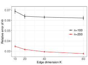
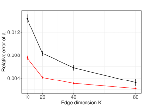
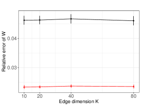
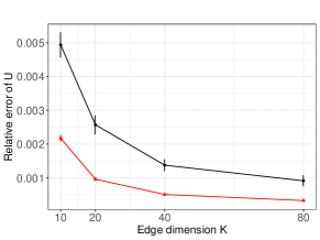
Figure 1: Mean relative errors and their corresponding $95\%$ intervals under varying $n$ and $K$, while $m=1$ and edge density at 0.08. The black and red lines mark $n=100$ and $n=200$, respectively.

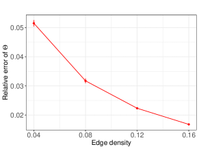
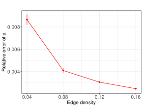
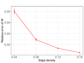
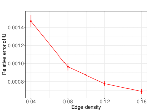
Figure 2: Mean relative errors and their corresponding $95\%$ intervals under varying edge density, while $n=200$, $K=20$ and $m=1$.

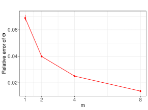
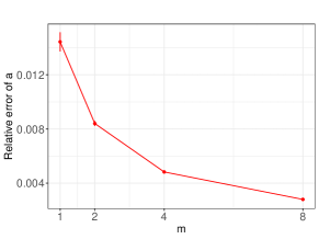
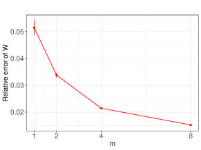
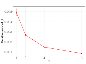
Figure 3: Mean relative errors and their corresponding $95\%$ intervals under varying $m$, while $n=200$, $K=20$ and edge density at 0.08.

It is seen from Figure 1 that estimation errors of ${\bm{a}}^{\ast}$ and ${\bm{U}}^{\ast}$ decrease with the network size $n$ and number of layers $K$, confirming the theoretical results in Theorem 1. The relative estimation error of ${\bm{W}}^{\ast}$ does not vary with $K$, as we rescale $\|\hat{\bm{W}}-\bm{W}^{\ast}\|_{F}^{2}$ by $\|\bm{W}^{\ast}\|_{F}^{2}$ in calculating the relative error and $\|\bm{W}^{\ast}\|_{F}^{2}$ scales with $K$. Additionally, Figures 2-3 show that as edge density, modulated by ${\bm{a}}^{\ast}$, and the number of edges $m$ increase, the estimation errors of ${\bm{a}}^{\ast}$, ${\bm{W}}^{\ast}$ and ${\bm{U}}^{\ast}$ decrease.

In our experiments, the edge cross-validation procedure performs well in selecting the latent position dimension $d$ and number of nonzero entries in ${\bm{W}}$. It consistently selects the correct $d$ across all simulation settings. Tables 1-2 report the TPR and FPR in estimating the nonzero entries in ${\bm{W}}^{\ast}$, with standard errors in the parentheses, over 100 data replications. It is seen that the variable selection accuracy improves with $n$, $m$ and edge density. The selection accuracy remains relatively stable across different numbers of layers $K$’s, which is expected given that the dimension of ${\bm{W}}$ increases with $K$.

Table 1: True Positive Rate (TPR) and False Positive Rate (FPR) in estimating ${\bm{W}}^{\ast}$ under varying $n$, $K$, while $m=1$ and edge density at 0.08.

	$n=100$				$n=200$
	$K=10$	$K=20$	$K=40$	$K=80$	$K=10$	$K=20$	$K=40$	$K=80$
TPR	0.880	0.881	0.883	0.882	0.910	0.925	0.919	0.921
	(0.045)	(0.034)	(0.028)	(0.023)	(0.039)	(0.031)	(0.024)	(0.027)
FPR	0.074	0.075	0.076	0.075	0.049	0.068	0.074	0.074
	(0.039)	(0.027)	(0.022)	(0.024)	(0.022)	(0.027)	(0.028)	(0.025)

Table 2: True Positive Rate (TPR) and False Positive Rate (FPR) in estimating ${\bm{W}}^{\ast}$ under varying edge density (while fixing $m=1$) and $m$ (while fixing edge density at 0.08).

	edge density				$m$
	$0.04$	$0.08$	$0.12$	$0.16$	$1$	$2$	$4$	$8$
TPR	0.850	0.925	0.970	0.986	0.880	0.915	0.948	0.962
	(0.045)	(0.031)	(0.007)	(0.003)	(0.045)	(0.035)	(0.021)	(0.019)
FPR	0.128	0.068	0.032	0.015	0.074	0.066	0.058	0.035
	(0.049)	(0.027)	(0.026)	(0.015)	(0.039)	(0.033)	(0.032)	(0.029)

6 Analysis of the Enron Email Network

6.1 Data description

The Enron email corpus (Klimt and Yang, 2004), one of the most extensive publicly available datasets of its kind, contains over 500,000 emails from 158 employees spanning from November 13, 1998 to June 21, 2002. Released by the Federal Energy Regulatory Commission following its investigation of Enron, this dataset provides a unique opportunity to study the communications and organizational structures within a major corporation during various stages of its financial collapse.

The study period of this dataset can be divided into three different stages, as marked by two major events. In February 2001, Enron’s stock reached its peak and then began a dramatic decline following major sell-offs from top executives. It was later found that starting February 2001, concerns about Enron’s accounting practices were increasingly discussed internally. In October 2001, the company’s financial scandal was publicly exposed and the Securities and Exchange Commission began an investigation into Enron’s accounting practices. Accordingly, we consider three stages in our analysis: the pre-decline period from November 13, 1998, to February 1, 2001; the decline and pre-bankruptcy period from February 1, 2001, to October 1, 2001; and the bankruptcy and post-bankruptcy period from October 1, 2001, to June 21, 2002.

Our analysis focused on the emails of 154 employees whose roles and departments are documented in the dataset. These employees are from different departments including Gas (ENA Gas), Legal (ENA Legal), Enron Transportation Services (ETS), Regulatory and Government Affairs and Enron Wholesale Services (EWS), among others. Data preparation included standard text preprocessing steps such as tokenization, lower-casing, removel of punctuations and stopwords, and stemming. We then employed Latent Dirichlet Allocation (LDA) to extract keywords that inform latent topics in the corpus. Table 3 shows the 45 extracted keywords. To construct the network for each stage, we merged all emails between each pair of nodes into a single document. This process created an undirected network with $n=154$ nodes and $K=45$ keywords for each stage, denoted by $\{y_{ij}^{(k)}\}_{i,j\in[154],k\in[45]}$, where $y_{ij}^{(k)}=y_{ji}^{(k)}=1$ if the merged document between users $i$ and $j$ includes keyword $k$, and $y_{ij}^{(k)}=y_{ji}^{(k)}=0$ otherwise. This approach helps to reduce the sparsity of the network and facilitates comparison with other multi-layer network analysis methods. The edge densities of the three networks constructed for Stages 1, 2, and 3 are 0.012, 0.010, and 0.009, respectively.

Keywords
Enron, corp, gas, power, energy, market, agreement,
information, price, deal, contract, credit, legal, fax, review,
capacity, phone, north, america,draft, texas, buy, trade,
discuss, risk, issue, position, letter, plan, stock,
natural, sell, value, customer, pipeline, product, continue,
cash, physical, pay, plant, account, picture, attach, earn

Table 3: Keywords extracted using LDA, sorted by their frequency of occurrences in the corpus.

6.2 Alternative approaches and link prediction

We also consider three alternative approaches when analyzing the Enron email network data:

• Separate: This method fits a separate latent space model to each layer, that is, $\bm{\Theta}^{(k)}={\bm{a}}^{(k)}\bm{1}_{n}^{T}+\bm{1}_{n}{{\bm{a}}^{(k)}}^{\top}+{\bm{U}}^{(k)}{{\bm{U}}^{(k)}}^{\top}$ for $k\in[K]$.

• Multiness (MacDonald et al., 2022): This method includes both a common latent structure across layers and a separate latent structure for each individual layer, written as $\bm{\Theta}^{(k)}=\bm{V}{\bm{I}}_{p_{0},q_{0}}\bm{V}^{\top}+{\bm{U}}^{(k)}{\bm{I}}_{p_{k},q_{k}}{{\bm{U}}^{(k)}}^{\top}$ for $k\in[K]$, where $\bm{V}\in\mathbb{R}^{n\times d_{0}}$ represents the matrix of common latent positions, ${\bm{U}}^{(k)}\in\mathbb{R}^{n\times d_{k}}$ collects the individual latent positions for layer $k$, and ${\bm{I}}_{p,q}=\left[\begin{array}[]{cc}{\bm{I}}_{p}&0\\ 0&-{\bm{I}}_{q}\end{array}\right].$

• FlexMn (Zhang et al., 2020b): This method considers a common latent position $\mathbf{U}$ across layers with a layer-specific scaling matrix $\mathbf{\Lambda^{(k)}}$, written as

  $$\bm{\Theta}^{(k)}={\bm{a}}^{(k)}\bm{1}_{n}^{\top}+\bm{1}_{n}{{\bm{a}}^{(k)}}^{\top}+{\bm{U}}\bm{\Lambda}^{(k)}{\bm{U}}^{\top},\text{ for }k\in[K],$$

  where ${\bm{a}}^{(k)}\in\mathbb{R}^{n}$, ${\bm{U}}\in\mathbb{R}^{n\times d}$, and $\bm{\Lambda}^{(k)}\in\mathbb{R}^{d\times d}$.

To ensure a fair comparison, edge cross-validation is used in selecting the latent position dimension for all above methods. We first compare the edge prediction accuracy and then examine the estimated latent positions from different methods. Comparisons of these methods in simulations are included in the Section S7 of supplement.

(a) Stage 1

(b) Stage 2

(c) Stage 3

Figure 4: Precision-Recall curves from different methods for out-of-sample link prediction.

Network link prediction is a fundamental task in network data analysis. To compare the performance of different methods, we randomly remove 20% entries from each layer and treat them as missing data. We then apply PLSM, Multiness, FlexMn, and Separate to the remaining entries and use the fitted model to predict link probabilities for the missing entries. This procedure is repeated 100 times. Figure 4 shows the average precision-recall curves from all four methods. It is seen that Separate does not perform well as it cannot borrow information across different layers; Multiness might have suffered from over-fitting as there is a large number of sparse layers in each of the three networks.

6.3 Estimation results from different methods

We apply our proposed method, PLSM, to the three networks from Stages 1-3 and use edge cross-validation to select the latent dimension $d$ and the sparsity $s$. The latent dimension $d$ was chosen as 10 for Stages 1 and 2, and 8 for Stage 3. The number of non-zero entries in ${\bm{W}}$ was selected as 6653, 6445, and 6237 for Stages 1, 2, and 3, respectively. Among the 154 employees, 43 held director-level or higher-level positions and had significantly more email correspondence. For visualization purposes, we focus on these 43 employees in Figures 5-6. The first row in Figure 5 plots the estimated latent node positions. The estimated latent position ${\bm{u}}_{i}$’s from PLSM are of unit length, placing them on a $K$-dimensional sphere. Two nodes with closer latent positions, i.e., having a smaller angle between them, are more likely to communicate. The clear clustering pattern of nodes in Stages 1 and 2 shows that before bankruptcy, executives in different departments function relatively autonomously. In Stage 3, there is a noticeable increase in cross-departmental communications. Also in Stage 3, we observe an increase in communications involving the Legal department (nodes from the Legal department move closer to others), likely due to the legal ramifications of bankruptcy proceedings.

Figure 5: Estimated latent positions by PLSM, FlexMn, and Multiness methods (top to bottom) and stages 1-3 (left to right). For Multiness, only the common latent positions are plotted.

For FlexMn, edge cross-validation selected latent dimensions of 9 for Stages 1 and 2, and 8 for Stage 3. Multiness, on the other hand, selected the maximum candidate value of 20 for the latent dimension $d$ for all three stages. The estimated latent positions from FlexMn and Multiness are shown in the second and third rows of Figure 5. For Multiness, only the common latent positions are plotted. Multiness displays similar qualitative patterns (up to a rotation) as PLSM in the estimated latent positions. In contrast, FlexMn appears less effective at distinguishing individuals from different departments in Stages 1 and 2.

Figure 6: Estimated preferential latent positions $[W_{1k}{\bm{u}}_{1},\ldots,W_{nk}{\bm{u}}_{n}]^{\top}$ by PLSM on keywords “legal”, “sell”, and “cash”.

In addition to the unit-length latent positions ${\bm{u}}_{i}$’s, PLSM also provides preferential latent positions calculated as $W_{ik}\mathbf{u}_{i}$’s for all $i,k$. For node $i$ on layer $k$, the direction of $W_{ik}\mathbf{u}_{i}$ is the same as ${\bm{u}}_{i}$, while its length $\|W_{ik}{\bm{u}}_{i}\|_{2}=W_{ik}$ characterizes the preference or activeness of node $i$ on layer $k$. Figure 6 shows the first three dimensions of $[W_{1k}{\bm{u}}_{1},\ldots,W_{nk}{\bm{u}}_{n}]^{\top}$. For illustration, we present the preferential latent positions for three keywords: “legal”, “sell”, and “cash.” The keyword “legal” in Enron email communications typically pertains to legal advice, agreements, regulatory issues, and discussions involving legal teams. The keyword “sell” generally involves discussions on asset transactions and marketing strategies. The keyword “cash” often relates to discussions on cash flow management and financial strategies. In Stage 1, the Legal department is more active in communications involving “legal” compared to “sell” or “cash”. Richard B. Sanders, Legal VP and Assistant General Counsel, exemplifies this focus. James D. Steffe, VP of Government Affairs and part of the Regulatory and Government Affairs (RGA) department, is seen active across all three layers in Stage 1. In contrast, Richard Shapiro, VP of Regulatory, shows less engagement in cash-related conversations, likely reflecting their differing responsibilities. John Arnold from the Gas department shows a significant interest in “sell” and engages more with the Legal and EWS departments in this context. Known as the “king of natural gas”, Arnold played a crucial role in natural gas trading and earned Enron’s largest bonus for his contributions. In Stage 2, the Gas and EWS departments are much closer compared to Stage 1, particularly in discussing legal-related issues. Aside from John Arnold, who remains actively engaged in both “sell” and “cash”, other members of the Gas and ETS departments show less activity. In Stage 3, the Legal department further increases its communication with other departments, especially in discussions related to cash-related issues. From Stages 2 to 3, there is a shift in interests within the RGA department, particularly for individuals such as Richard Shapiro (VP of Regulatory Affairs) and James D. Steffes (VP of Government Affairs). Both moved closer to other departments regarding “legal” matters, likely due to their involvement in post-bankruptcy issues. Additionally, the Legal department’s activity in “cash” discussions decreased.

(a) “legal”

(b) “cash”

Figure 7: Boxplots of $W_{ik}$’s for “legal” and “cash” for nodes from different departments.

Figure 7 plots individual preferences $W_{ik}$’s for “legal” and “cash” by departments. It is seen from the left plot that the Legal and RGA departments are consistently active in legal-related issues across all three stages. Meanwhile, Gas and ETS departments had low activity in legal-related issues in Stages 1-2, and showed a noticeable increase in their activity in Stage 3, likely due to a stronger focus on legal-related issues following the bankruptcy. Additionally, within the EWS department, there is an observed increase in the variability of interest levels in legal-related matters from Stage 1 to Stage 3. The right plot of Figure 7 shows a noticeable increase in interest regarding cash-related issues in Stage 3 from the Gas, ETS, and EWS departments. Following the company’s bankruptcy, communications within these departments frequently include terms such as “cash out” and “cash crunch”. In contrast, the Legal and RGA departments show significantly decreased interest in cash-related issues in Stage 3.

One attractive feature of our method is that it can offer the above insights on node preferences for different keywords, offering detailed perspectives that are not directly available from other methods.

7 Discussion

In this work, we propose a new and flexible preferential latent space model that can offer direct insights on how contents of the textual exchanges modulate the relationships between nodes. We establish identifiability conditions for the proposed model and tackle model estimation using a computationally efficient projected gradient descent algorithm. We further establish the non-asymptotic error bound for the estimator from each step of the algorithm, where we derive a sharp spectral concentration bound that may be of independent interest.

Our work can be naturally extended in several directions. One interesting direction is to extend the proposed modeling framework to directed networks. This involves deriving new identifiability conditions and modifying the proposed algorithm. Our work can also be extended to incorporate node-level and/or edge-level covariates. This direction can be developed following the approach in Ma et al. (2020). We leave these directions to future research.

References

- Athreya et al. (2018) Athreya, A., Fishkind, D. E., Tang, M., Priebe, C. E., Park, Y., Vogelstein, J. T., Levin, K., Lyzinski, V., Qin, Y., and Sussman, D. L. (2018), “Statistical inference on random dot product graphs: a survey,” Journal of Machine Learning Research, 18, 1–92.
- Borgatti et al. (2009) Borgatti, S. P., Mehra, A., Brass, D. J., and Labianca, G. (2009), “Network analysis in the social sciences,” science, 323, 892–895.
- Bota et al. (2003) Bota, M., Dong, H.-W., and Swanson, L. W. (2003), “From gene networks to brain networks,” Nature neuroscience, 6, 795–799.
- Boutin et al. (2023) Boutin, R., Bouveyron, C., and Latouche, P. (2023), “Embedded topics in the stochastic block model,” Statistics and Computing, 33, 95.
- Bouveyron et al. (2018) Bouveyron, C., Latouche, P., and Zreik, R. (2018), “The stochastic topic block model for the clustering of vertices in networks with textual edges,” Statistics and Computing, 28, 11–31.
- Corneli et al. (2019) Corneli, M., Bouveyron, C., Latouche, P., and Rossi, F. (2019), “The dynamic stochastic topic block model for dynamic networks with textual edges,” Statistics and Computing, 29, 677–695.
- Devlin et al. (2018) Devlin, J., Chang, M.-W., Lee, K., and Toutanova, K. (2018), “Bert: Pre-training of deep bidirectional transformers for language understanding,” arXiv preprint arXiv:1810.04805.
- D’Angelo et al. (2019) D’Angelo, S., Murphy, T. B., and Alfò, M. (2019), “Latent space modelling of multidimensional networks with application to the exchange of votes in eurovision song contest,” The Annals of Applied Statistics, 13, 900–930.
- Elliott et al. (2014) Elliott, M., Golub, B., and Jackson, M. O. (2014), “Financial networks and contagion,” American Economic Review, 104, 3115–3153.
- Frank and Strauss (1986) Frank, O. and Strauss, D. (1986), “Markov graphs,” Journal of the American Statistical Association, 81, 832–842.
- Gollini and Murphy (2016) Gollini, I. and Murphy, T. B. (2016), “Joint modeling of multiple network views,” Journal of Computational and Graphical Statistics, 25, 246–265.
- Hoff et al. (2002) Hoff, P. D., Raftery, A. E., and Handcock, M. S. (2002), “Latent space approaches to social network analysis,” Journal of the American Statistical Association, 97, 1090–1098.
- Jing et al. (2021) Jing, B.-Y., Li, T., Lyu, Z., and Xia, D. (2021), “Community detection on mixture multilayer networks via regularized tensor decomposition,” The Annals of Statistics, 49, 3181–3205.
- Joachims (1998) Joachims, T. (1998), “Text categorization with support vector machines: Learning with many relevant features,” in European conference on machine learning, Springer, pp. 137–142.
- Ke et al. (2023) Ke, Z. T., Ji, P., Jin, J., and Li, W. (2023), “Recent advances in text analysis,” Annual Review of Statistics and Its Application, 11.
- Klimt and Yang (2004) Klimt, B. and Yang, Y. (2004), “The Enron Corpus: A New Dataset for Email Classification Research,” in Machine Learning: ECML 2004, eds. Boulicaut, J.-F., Esposito, F., Giannotti, F., and Pedreschi, D., Berlin, Heidelberg: Springer Berlin Heidelberg, pp. 217–226.
- Lei et al. (2020) Lei, J., Chen, K., and Lynch, B. (2020), “Consistent community detection in multi-layer network data,” Biometrika, 107, 61–73.
- Lei and Lin (2023) Lei, J. and Lin, K. Z. (2023), “Bias-adjusted spectral clustering in multi-layer stochastic block models,” Journal of the American Statistical Association, 118, 2433–2445.
- Lei and Rinaldo (2015) Lei, J. and Rinaldo, A. (2015), “Consistency of spectral clustering in stochastic block models,” The Annals of Statistics, 43, 215–237.
- Li et al. (2020) Li, T., Levina, E., and Zhu, J. (2020), “Network cross-validation by edge sampling,” Biometrika, 107, 257–276.
- Lyu et al. (2023) Lyu, Z., Li, T., and Xia, D. (2023), “Optimal Clustering of Discrete Mixtures: Binomial, Poisson, Block Models, and Multi-layer Networks,” arXiv preprint arXiv:2311.15598.
- Ma et al. (2020) Ma, Z., Ma, Z., and Yuan, H. (2020), “Universal latent space model fitting for large networks with edge covariates,” Journal of Machine Learning Research, 21, 86–152.
- MacDonald et al. (2022) MacDonald, P. W., Levina, E., and Zhu, J. (2022), “Latent space models for multiplex networks with shared structure,” Biometrika, 109, 683–706.
- Mihalcea and Tarau (2004) Mihalcea, R. and Tarau, P. (2004), “Textrank: Bringing order into text,” in Proceedings of the 2004 conference on empirical methods in natural language processing, pp. 404–411.
- Mikolov et al. (2013) Mikolov, T., Chen, K., Corrado, G., and Dean, J. (2013), “Efficient estimation of word representations in vector space,” arXiv preprint arXiv:1301.3781.
- Nowicki and Snijders (2001) Nowicki, K. and Snijders, T. A. B. (2001), “Estimation and prediction for stochastic blockstructures,” Journal of the American Statistical Association, 96, 1077–1087.
- Paul and Chen (2020) Paul, S. and Chen, Y. (2020), “Spectral and matrix factorization methods for consistent community detection in multi-layer networks,” The Annals of Statistics, 48, 230–250.
- Sachan et al. (2012) Sachan, M., Contractor, D., Faruquie, T. A., and Subramaniam, L. V. (2012), “Using content and interactions for discovering communities in social networks,” in Proceedings of the 21st international conference on World Wide Web, pp. 331–340.
- Salter-Townshend and McCormick (2017) Salter-Townshend, M. and McCormick, T. H. (2017), “Latent space models for multiview network data,” The Annals of Applied Statistics, 11, 1217.
- Tropp (2012) Tropp, J. A. (2012), “User-friendly tail bounds for sums of random matrices,” Foundations of computational mathematics, 12, 389–434.
- Wang and Wong (1987) Wang, Y. J. and Wong, G. Y. (1987), “Stochastic blockmodels for directed graphs,” Journal of the American Statistical Association, 82, 8–19.
- Zhang and Chen (2015) Zhang, J. and Chen, Y. (2015), “Exponential random graph models for networks resilient to targeted attacks,” Statistics and its Interface, 8, 267–276.
- Zhang et al. (2020a) Zhang, J., Sun, W. W., and Li, L. (2020a), “Mixed-effect time-varying network model and application in brain connectivity analysis,” Journal of the American Statistical Association, 115, 2022–2036.
- Zhang et al. (2023) Zhang, J., Sun, W. W., and Li, L. (2023), “Generalized connectivity matrix response regression with applications in brain connectivity studies,” Journal of Computational and Graphical Statistics, 32, 252–262.
- Zhang et al. (2020b) Zhang, X., Xue, S., and Zhu, J. (2020b), “A flexible latent space model for multilayer networks,” in International Conference on Machine Learning, PMLR, pp. 11288–11297.
- Zhou et al. (2006) Zhou, D., Manavoglu, E., Li, J., Giles, C. L., and Zha, H. (2006), “Probabilistic models for discovering e-communities,” in Proceedings of the 15th international conference on World Wide Web, pp. 173–182.