Input-driven circuit reconfiguration in critical recurrent neural networks.

Abstract

Changing a circuit dynamically, without actually changing the hardware itself, is called reconfiguration, and is of great importance due to its manifold technological applications. Circuit reconfiguration appears to be a feature of the cerebral cortex, and hence understanding the neuroarchitectural and dynamical features underlying self-reconfiguration may prove key to elucidate brain function. We present a very simple single-layer recurrent network, whose signal pathways can be reconfigured “on the fly” using only its inputs, with no changes to its synaptic weights. We use the low spatio-temporal frequencies of the input to landscape the ongoing activity, which in turn permits or denies the propagation of traveling waves. This mechanism uses the inherent properties of dynamically-critical systems, which we guarantee through unitary convolution kernels. We show this network solves the classical connectedness problem, by allowing signal propagation only along the regions to be evaluated for connectedness and forbidding it elsewhere.

The brain changes its own hardware at different timescales, for example through synaptic plasticity, synaptic remodeling and adult neurogenesis [1], and thus retains an extraordinary amount of long-term plasticity. But also, some brain areas evidence the ability to switch between several different functions depending on context, and these switches happen at faster speeds that seem compatible with a physical change in the underlying neural substrate [2, 3]. Hence it is now appreciated that the brain dynamically reconfigures its operations without physical reconfiguration [4]. One potential mechanism that has been strongly implicated in such rapid reconfigurations is ongoing brain activity [5], for example ongoing traveling waves [6]. Hence, as advocated in [4] it is fundamental to understand the dynamical principles through which a complex network can reconfigure its operations, by managing and curating its own dynamical state.

I shall show below that critical dynamics, through its inherent singular dependence of the dynamical state on the input, allows a network to be reconfigured rapidly and efficiently by suitable choice of inputs. The inputs to such a network conceptually contain both external sensory information as well as instructions from other brain areas. Information flows through such a network along pathways which can be dynamically changed, with no changes to the synaptic weights, and without any “special circuitry” being involved. I shall construct an example, the simplest I could manage, where the input contains both control and signaling components in separate spatiotemporal bands. The control component (low spatial and temporal frequencies) will literally be an image of walls and channels; the signaling component (higher temporal frequencies) will consist of point-wise signal sources generating traveling waves; these waves will freely propagate through the channels but will exponentially attenuate into the walls, or even reflect off of them. As they do, they will propagate into every place that’s allowed by the input, implementing de facto a floodfill (“paint bucket”) algorithm. This relates to a classical problem: how do our brains detect connectedness of areas in visual stimuli [7, 8], a problem which is arguably not solvable by feedforward architectures of fixed depth. It is argued cogently in [9] that this is in fact a touchstone for the central role of recurrence in the nervous system.

I will use a single-layer recurrent convolutional neural network with unitary (critical) coupling kernel. The family of such networks was derived as a Poincaré map from critical ODEs in [10], and their basic dynamical analysis is outlined in [11] and [12]. The state is given by a complex-valued “neural” layer $Z$, henceforth a lattice of complex numbers in either 1 or 2 dimensions with periodic boundary conditions. Its evolution in time is denoted as $Z_{n}$ where $n$ is (integer) time, through the recursion

$$Z_{n+1}=\phi\left(U\otimes Z_{n}+I_{n}\right)$$ (1)

where $\otimes$ is the convolution operation natural to $Z$; $U$ is a (unitary) convolution kernel; $I_{n}$ is a sequence of external inputs of the same shape as $Z$; and $\phi$ is a smooth, scalar “activation function” operating element-wise on $Z.$ A natural choice of $\phi$ for this construction is $\phi(z)=z/\sqrt{1+|z|^{2}}$, a complex-valued phase-preserving sigmoid [12]. We choose $U$ to be a unitary kernel, i.e. its associated linear operator’s eigenvalues $\lambda$ lie on the unit circle: $|\lambda|=1$. We generate unitary convolution kernels by convolutional exponentiation of an anti-Hermitic kernel [11]:

$$U=e_{\otimes}^{A}\equiv\mathscr{F}^{-1}\left\{\exp\left(\mathscr{F}\left\{A\right\}\right)\right\}$$ (2)

where the exponential is element-wise, $\mathscr{F}$ and $\mathscr{F}^{-1}$ the direct and inverse Fourier transforms in the dimension $D$ appropriate to $Z$ and $K$, and $A^{\dagger}=-A$, i.e. antiHermitic.

Finally, we remind the reader that the eigenvalues of a convolution with a kernel $U$ are the individual elements of the Fourier transform of $U$, and the corresponding eigenvectors are the Fourier modes associated to those elements. The Fourier transform of the kernel $A$ giving rise to $U$ is is called the dispersion relation of the kernel; since it is purely imaginary, it associates a non-decaying frequency to each wavenumber.

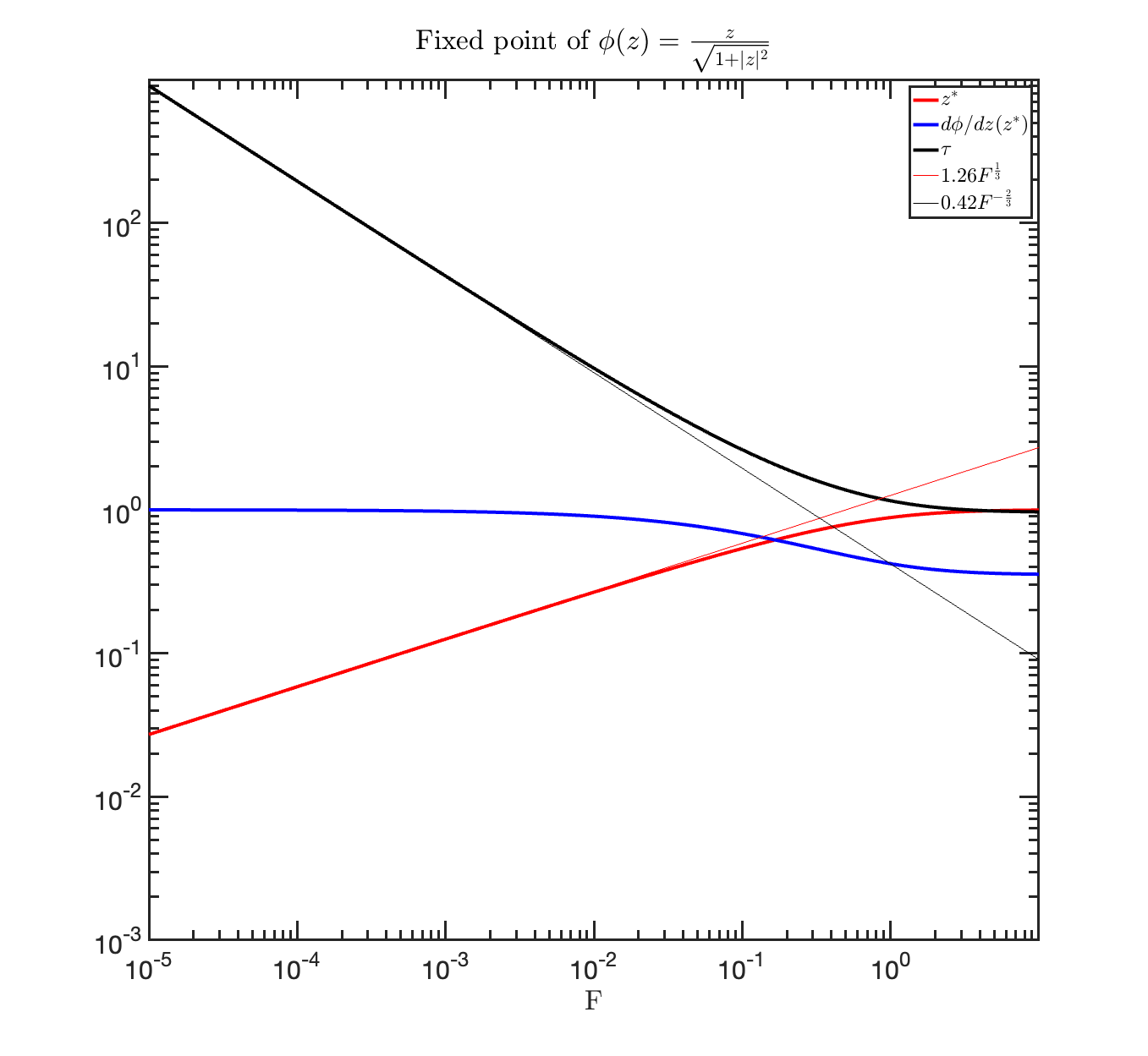
Figure 1: From [12]. The fixed point $z_{*}=\phi(z_{*}+I)$ with $\phi(z)=z/\sqrt{1+z^{2}}$; $z_{*}$ as a function of $I$ (red), together with $\phi^{\prime}(z_{*})=\left(1+z_{*}^{2}\right){}^{-\frac{2}{3}}$, the slope of $\phi$ at the fixed point controlling decay rate (blue), and $-1/\log(\phi^{\prime}(z_{*}))$ (black), the relaxation time to the fixed point. The thin lines are power-law asymptotics to the low $I$ regime: $z_{*}\approx\left(2I\right)^{\frac{{1}}{3}}$ and $\tau\approx\frac{2}{3}\left(2I\right)^{-\frac{{2}}{3}}$.

The propagation of perturbations through this system can be analyzed in terms of linear stability of dynamical systems. The derivative of the state $Z_{n}$ at time $n$ wrt the initial state $Z_{0}$ at time $0$ telescopes through the chain rule into a product of derivatives [19, 20], each one of which contains two terms: the constant unitary matrix representing the action of the convolution with $U$ (denoted by $[U\otimes]$ in [11]), times the matrix of derivatives of $\phi$ evaluated at its argument at the appropriate time-step, which, since $\phi$ is element-wise, is strictly diagonal:

$$\frac{\partial Z_{n}}{\partial Z_{0}}\approx\prod_{i=0}^{n-1}\Gamma_{i}\cdot[U\otimes]\quad{\rm where}\quad\Gamma_{i}\doteq{\rm diag}\left[\phi^{\prime}(MZ_{i}+I_{i})\right]$$

If $\phi$ is a sigmoidal function, and satisfies $\phi^{\prime}(0)=1$ and $0\leq\phi^{\prime}(x\neq 0)<1$, then for $I=0$: (a) the state $Z\equiv 0$ is globally attracting (i.e. all activities in the layer decay to $0$ regardless of initial conditions), and (b) the system is “critical” in that the derivative above is a power of the constant unitary matrix and thus unitary itself. Unitarity of the coupling matrix has manifold other implications beyond the dynamical ones we explore here. In particular unitary couplings have been employed in the ANN literature [15] as a means to overcome the vanishing gradient problem [16]. The fact that the same matrix $\Lambda\cdot[U\otimes]$ controls both asymptotic stability as well as back-propagation is a connection that will be explored elsewhere.

For $\phi(z)=z/\sqrt{1+|z|^{2}}$ the response to input forcing at the same frequency as an eigenvalue of $K$ results, as shown in [12], in the singular nonlinear cubic-root compression characteristic of the forced Hopf bifurcation [13, 14] wherein the amplitude of the response is proportional to the cubic root of the amplitude of the input when driven exactly at resonance.b We will illustrate in a scalar example:

$$z_{n+1}=\phi(z_{n}+I_{n})=\frac{(z_{n}+I_{n})}{\sqrt{1+\left(z_{n}^{2}+I_{n}\right)}}$$

where $z$ is now a single complex number. For constant $I$, this recurrence converges to a fixed point given by $\left(z_{*}+I\right)^{2}=\frac{z_{*}^{2}}{1-z_{*}^{2}}$ from where asymptotically $z_{*}=(2I)^{1/3}$. Perturbations around $z_{*}$ evolve, to linear order, through powers of $\phi^{\prime}(z_{*}+I)$:

$$z^{*}+\delta_{n+1}=\phi(z^{*}+I+\delta_{n})\approx\phi(z^{*}+I)+\phi^{\prime}(z^{*}+I)\delta_{n}$$

See Figure 1.

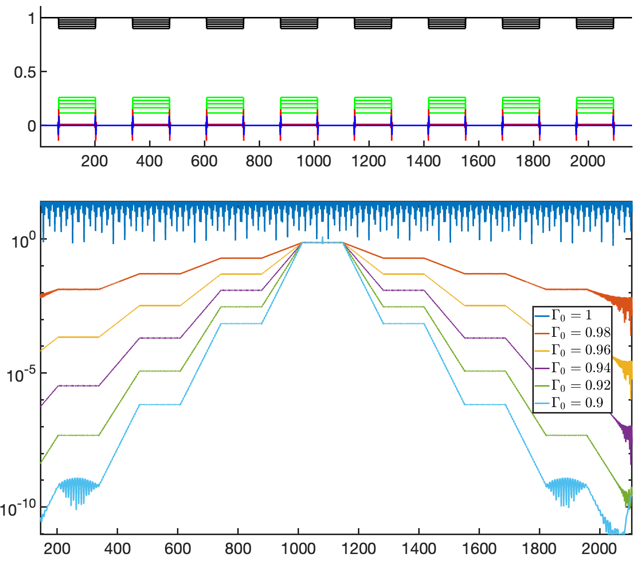
Figure 2: 1D network (N=2048). Top panel. $\Gamma$ (top line, black) was chosen to have 8 alternating cycles between $\Gamma=1$ and $\Gamma=\Gamma_{0}$. From there $Z_{*}$ is computed (green line) and then $I_{0}$ (real part, red; imaginary part, blue). Bottom panel: An oscillatory signal is injected at the center (a non-attenuating region) and propagates outwards. Notice it exponentially decays as it traverses $\Gamma<1$ areas and does not attenuate through $\Gamma=1$ areas.

We now carry this out in a spatially extended system. We first review the case already considered in [12]: a spatially and temporally constant input generates a steady state; an oscillatory perturbation injected into a single site generates waves that propagate outwards from the injection site and attenuate as they do. The constant component creates “ongoing activity”, and the operating point of the dynamical system shifts to values of $Z$ for which the derivative of $\phi$ is no longer 1. The oscillatory input then propagates against this background.

We write the input as $I_{n}=I_{0}+\alpha\lambda^{n}\delta_{0}$, where $I_{0}$ is a spatially and temporally constant input, $\lambda=e^{i\theta}$, and $\delta_{0}$ the image with a single $1$ at element $(0,0)$. Following standard dynamical-systems perturbation analysis, we will analyze the behavior around $\alpha\to 0$, and so henceforth we assume $\alpha\ll Z^{*}$. For $\alpha=0$ our system reaches a steady state given by

$$Z^{*}=\phi(U\otimes Z^{*}+I_{0})$$ (3)

where it follows that $Z^{*}$ is spatially and temporally constant. See also Figure 1.

For $\alpha\neq 0$ we write $Z_{n}=Z^{*}+\Delta Z_{n}$ into 1 to obtain

$$Z^{*}+\Delta Z_{n+1}=\phi(U\otimes Z^{*}+U\otimes\Delta Z_{n}+I_{0}+\alpha\lambda^{n}\delta_{0})$$

and expanding the RHS to first order we obtain

$$Z^{*}+\Delta Z_{n+1} = \phi(U\otimes Z^{*}+I_{0})+\cdots$$

$$+ \phi^{\prime}(U\otimes Z^{*}+I_{0})\left(U\otimes\Delta Z_{n}+\alpha\lambda^{n}\delta_{0}\right)$$

the first terms in both the right-hand side and left-hand side cancel, and calling $\Gamma$ the value

$$\Gamma=\phi^{\prime}(U\otimes Z^{*}+I_{0})=\phi^{\prime}(\phi^{-1}(Z^{*}))$$ (5)

we reach a linear propagation equation for the perturbation generated by the oscillatory input:

$$\Delta Z_{n+1}=\Gamma\cdot\left\{U\otimes\Delta Z_{n}+\alpha\lambda^{n}\delta_{0}\right\}$$ (6)

from where we see that the wave generated by the oscillatory input attenuates by a factor of $\Gamma$ every time-step. This temporal attenuation then transforms into a spatial attenuation due to the finite speed of propagation of the wave (its group velocity): the slower the wave, the many more factors of $\Gamma$ are incurred in traversing a given distance. As shown in [12] the asymptotic state for this equation can be computed in closed form. Writing $\Delta Z_{n}=R^{*}\lambda^{n}$ and substituting in the equation above we get $R^{*}\lambda=\Gamma(U\otimes R^{*}+\alpha\delta_{0})$, an equation which is explicitly solvable in Fourier space

$$R^{*}=\mathscr{F}^{-1}\left[\cdot\frac{\alpha\mathbf{\mathscr{F}[\delta_{0}]}}{\lambda/\Gamma-\mathscr{F}[U]}\right]$$

where $\cdot-$ denotes pointwise division. For $\Gamma\to 1$ as $\lambda$ approaches an eigenvalue of $U$ (these are, in fact, the elements of $\mathscr{F}[U]$ and are, as discussed arranged on the unit complex circle) the denominator has a pole and the corresponding eigenvector dominates $R^{*}$, but for $\Gamma<1$ the denominator is bounded away from $0$ and the responses are spatially-decaying exponentials around the injection point.

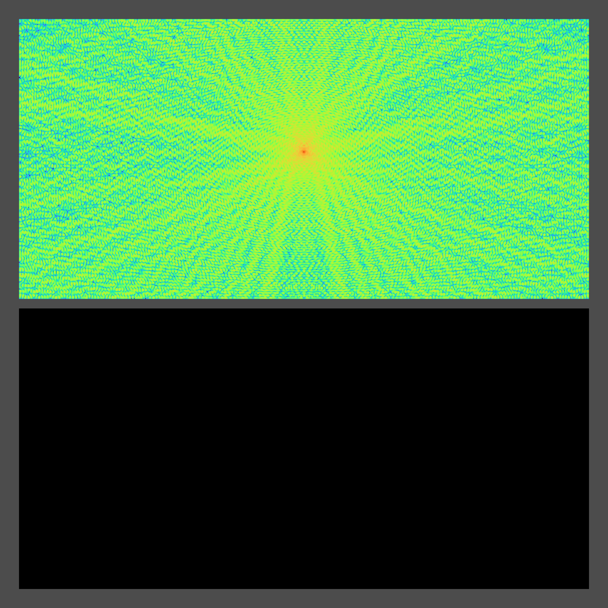
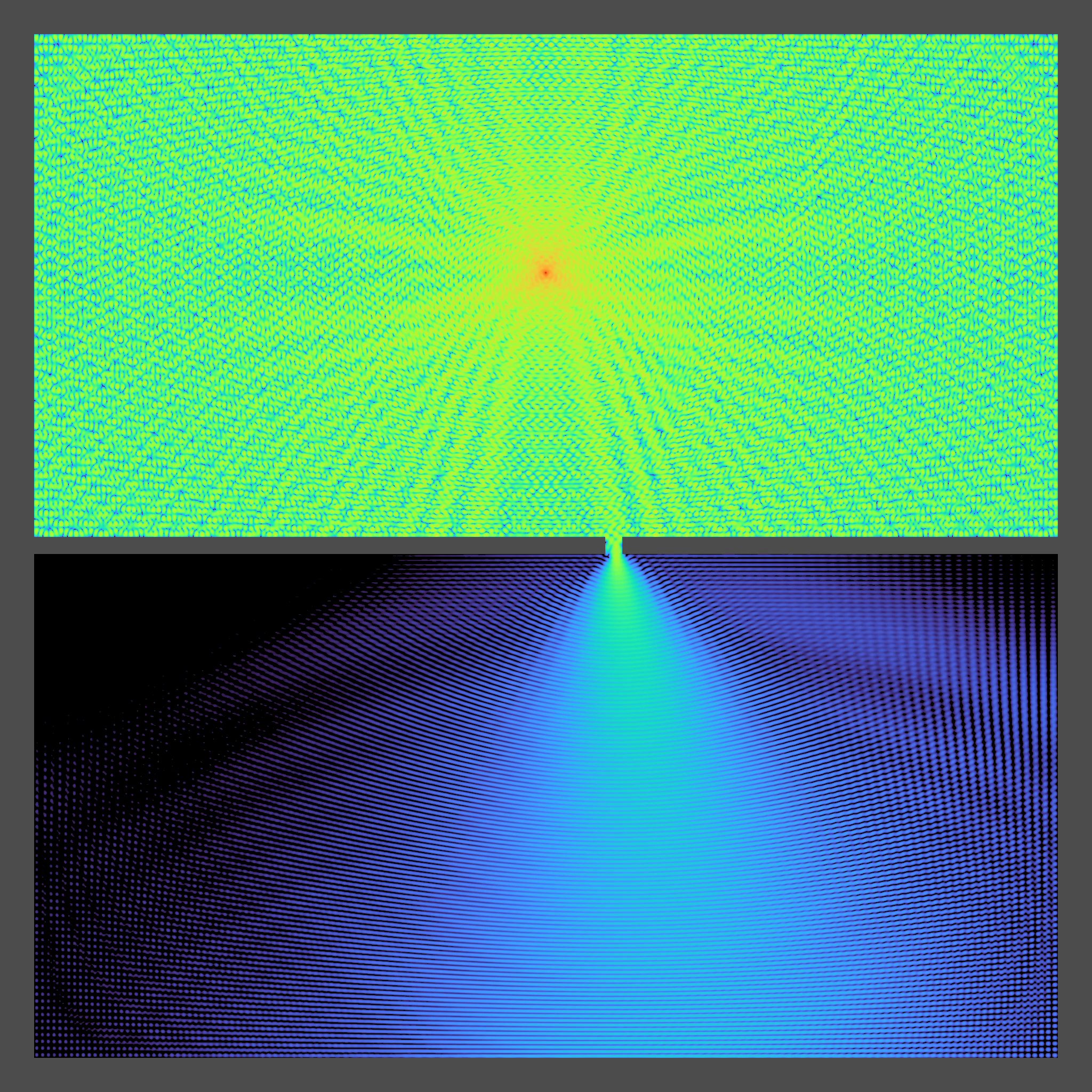
Figure 3: Two vertically-stacked boxes. The gray areas cannot be traversed. In addition to the input $I_{0}$ patterning the boxes, an additional oscillatory input is applied at the center of the top box. Left, the middle wall is intact; the signal injected at the top box stays in the top box. Center, a small aperture is broken in the middle wall; the signal leaks into the bottom box. Full movies in Supp Mat. This demonstrates the walls act as a geometric IF statement: something is allowed to happen or not depending on an input.

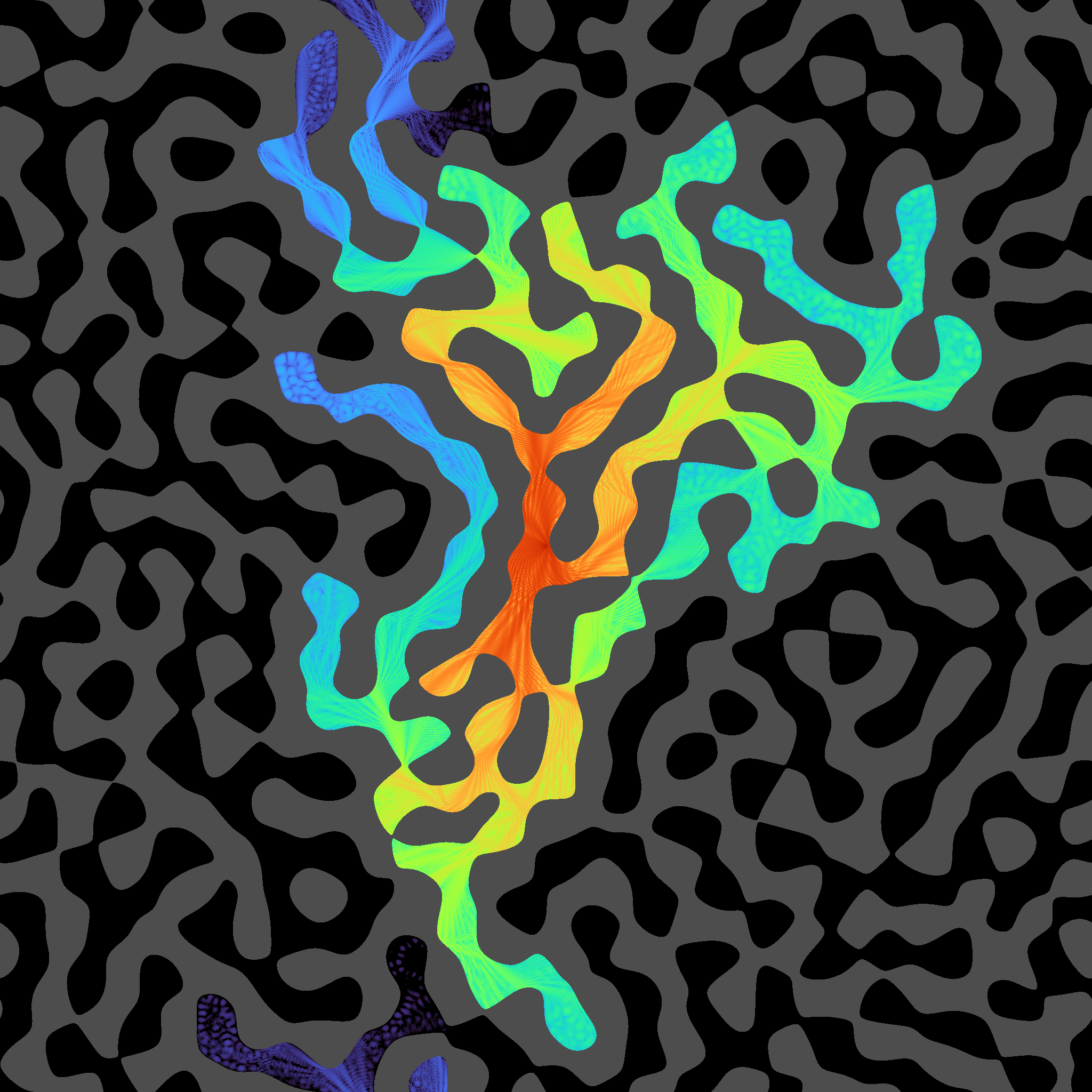
Figure 4: A labyrinthine pattern was created using band-passed noise to pattern areas where propagation is allowed ($\Gamma=1$, in black) or strongly disallowed ($\Gamma=0.01$, gray). An oscillating signal at the frequency of an eigenvalue was then injected at a single pixel the center of the figure; the network was evolved and this figure shows $\log(|Z|)$ in color code. $Z$ is a 2048x2048 long complex array; $U$ is the exponential of a numerical Laplacian kernel (times $i$). Please notice that the oscillatory signal did not fill non-contiguous areas, implementing the classic floodfill algorithm (a.k.a. paint bucket). Full movies are in Supplementary Materials

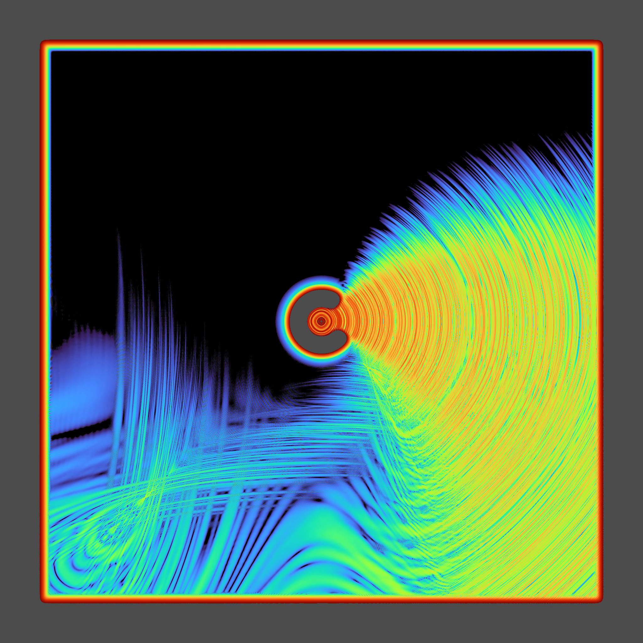
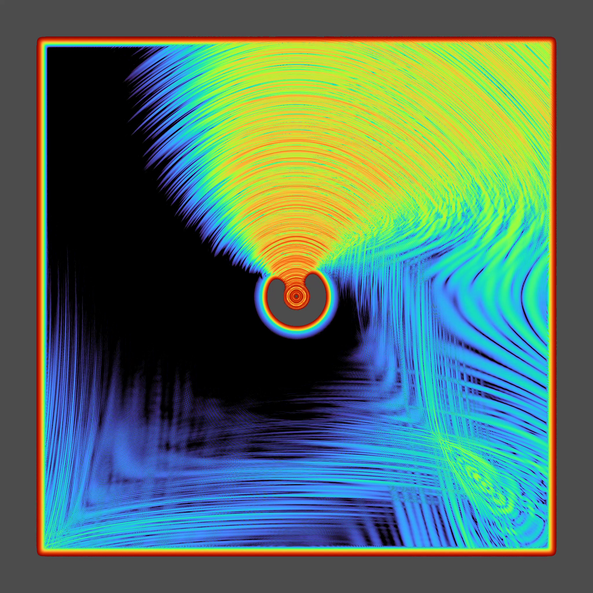
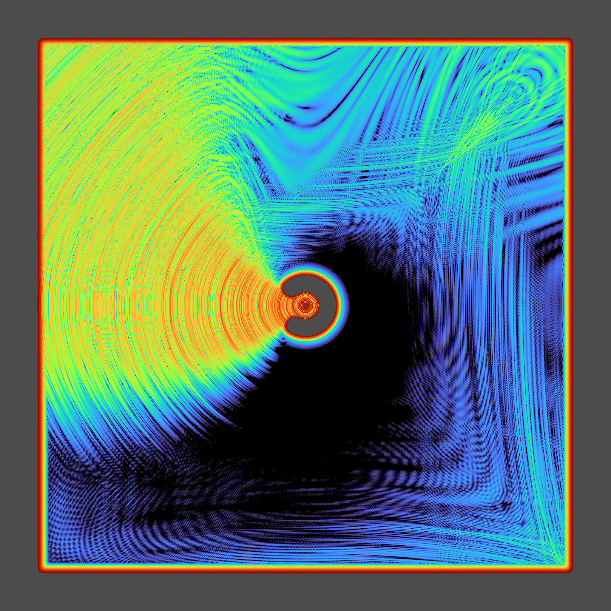
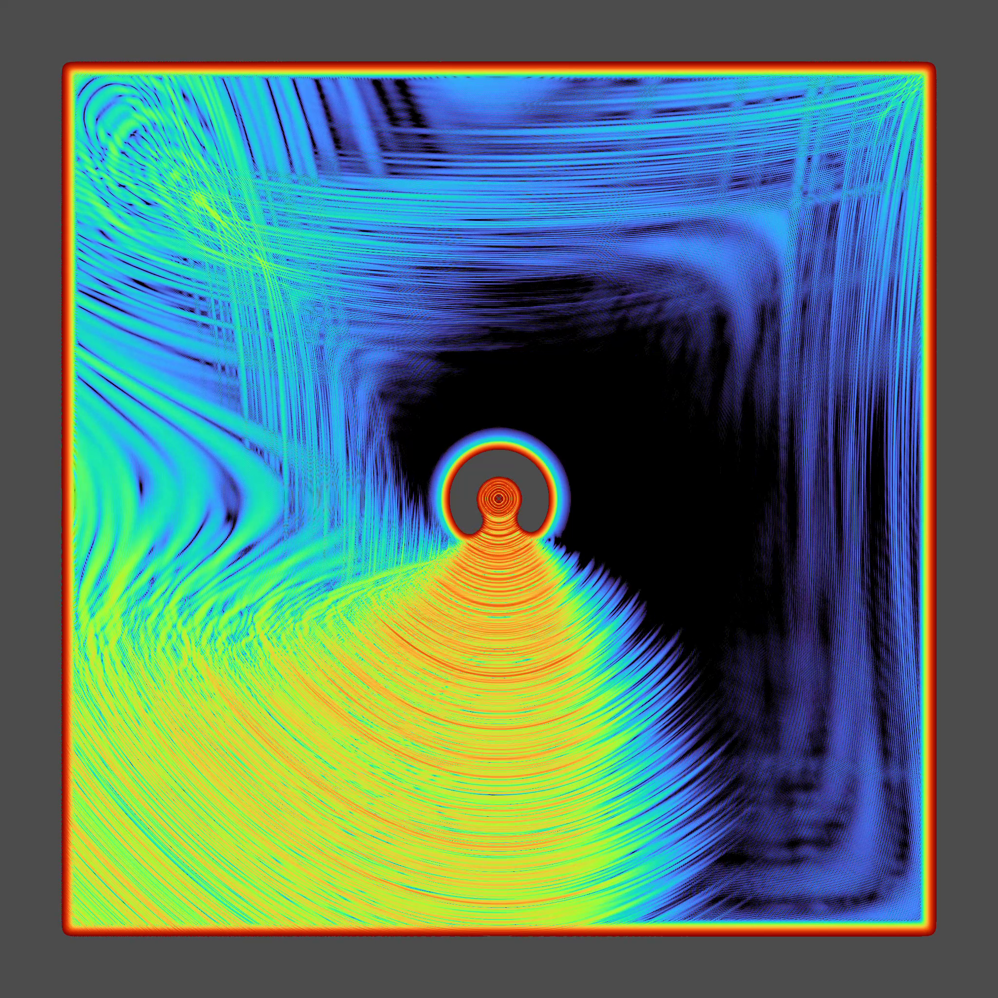
Figure 5: Lighthouse.

The previous discussion suggests to use a spatially varying $I_{0}$ to spatially pattern areas where a signal is not allowed to enter and others where it is free to propagate. Given a temporally constant but spatially-patterned input $I^{*}$, iteration of Eq 1 will reach a spatial pattern of ongoing activity $Z^{*}$ given by the fixed point Eq 3. Perturbations around the fixed point evolve according to Eq 6, through the derivative of the activation function $\phi$ evaluated at its arguments $U\otimes Z^{*}+I_{0}$; this derivative $\Gamma\doteq\phi^{\prime}(U\otimes Z^{*}+I_{0})$ is now spatially patterned and will generate areas of unobstructed wave propagation wherever $|\Gamma|=1$, wave absorption whenever $|\Gamma|<1$, wave amplification and regeneration when $|\Gamma|>1$, and complex scattering effects when the phase of $\Gamma$ varies spatially.

To engineer a given outcome we have to work our way backwards through the equations: from the desired $\Gamma,$ compute the $Z^{*}$ that gives rise to $\Gamma$, then compute the $I^{*}$ that gives rise to $Z^{*}$. Start with the construction of a desired spatially-varying $\Gamma$: this is an array, the same size as the layer $Z$, and wherever $|\Gamma|=1$ waves propagate unhindered, and wherever $|\Gamma|<1$ waves attenuate. Then we invert Eq 5 to get the arguments of $\phi^{\prime}$ as a function of $\Gamma$. For our choice of $\phi,$ we have $\phi^{\prime}(z)=\left(1+z^{2}\right)^{-3/2}$ so $z=\sqrt{\phi^{\prime-2/3}-1}$ and thus

$$U\otimes Z^{*}+I_{0}=\sqrt{\Gamma^{-2/3}-1}$$

This gives us both the ongoing activity and the input as a function of $\Gamma$. To simplify we note that the entire LHS of this equation is the argument to $\phi$ in Eq 3: apply $\phi$ to both sides and substitute 3 to solve for $Z^{*}$ only as a function of $\Gamma$:

$$Z^{*}=\phi\left(\sqrt{\Gamma^{-2/3}-1}\right)$$

and then finally use again Eq 3 to solve for what the input is that gives rise to a given ongoing activity: $I_{0}=\phi^{-1}\left(Z^{*}\right)-U\otimes Z^{*}$

$$I_{0}=\sqrt{\Gamma^{-2/3}-1}-U\otimes\left[\phi\left(\sqrt{\Gamma^{-2/3}-1}\right)\right]$$ (7)

Equation 7 is our central result. Using this equation, we can obtain any desired pattern of spatial attenuation.

To illustrate how input can be used to generate or open barrierts to passage, in Figure 3, we used a (complex) layer $Z$ of size 2048x2048, and $U=e_{\otimes}^{i\Delta}$ with $\Delta$ a numerical Laplacian kernel. An array $\Gamma$ was created defining two boxes stacked over each other; the walls of these boxes are strongly attenuating and cannot be traversed by signals, and the $I_{0}$ was computed. An oscillatory signal was then added to $I_{0}$ applied at a single pixel at the center of the top box. When the wall between the boxes is intact, the signal at the top cannot reach the bottom box. If, on the other hand, a small hole is made in the middle wall, then the signal can reach the bottom. Therefore, this shows how the input signal $\Gamma$ can change whether or not other signals are able to propagate; in effect, this is a geometric IF statement that allows something to happen or not happen depending on what the input is.

In Figure 4, we used a complex-valued 2048x2048 layer $Z$; created a labyrinthine pattern for $\Gamma$ (using thresholded band-pass noise) and computed the $I_{0}$ and $Z^{*}$ that generate it; then an oscillatory signal was applied at the center of $Z$ and allowed to propagate. The signal propagates only along the allowed channels, filling contiguous regions but not invading non-contiguous regions, thus implementing floodfill, a computation that, as discussed in the introduction, has been shown not to be computable using feedforward networks [7, 8].

To illustrate how to use a moving boundary condition, in Figure 5 we used as an input, a slowly rotating image of $3/4$ of an annulus (i.e. an annulus with one quarter missing) as our impenetrable wall, and placed a signal source at its center. As a result, the signal escapes the annulus through the opening, which then rotates. forming a little “lighthouse”. This shows input-dependent directional selection of a signal, or dynamic routing.

To conclude, we have presented a fairly minimal model of dynamic reconfiguration. The model is inherently geometrical, because it is laid out on an Euclidean lattice supporting convolutions, but illustrates concepts that can be used on more complex underlying topologies: (a) to use connections that support travelling waves, by use of unitary dynamics, (b) to exploit the inherent sensitivity of such a system to sculpt ongoing activity, (c) use that activity to control the space through which the travelling waves can move in a dynamical fashion. This mechanism can be viewed as a geometric form of an IF statement: depending on some data, a computation is carried out, or not. The ways that such a geometrical construct can be exploited are undoubtedly numerous.

We make no representation that this model is optimal in any way other than being conceptually simple, nor we make a claim that it is directly applicable to computational neuroscience other than illustrating a dynamical mechanism. No effort was made to optimize any of the available degrees of freedom: the kernel, the activation function, and the patterns used as input. It is clear that a designed or optimized network could do materially better at the tasks presented. The virtue of this model is one: Figs 3,4, and 5 were run on the same, identical network: same kernel, same activation. The only thing that changes between them is the input $I^{*}$ given to pattern the tasks. (Supplementary Movie 7 shows dynamics with a random 7x7 kernel, to illustrate the fact that the results are not sensitive to the choice of kernel).

I would like to acknowledge the late Hector Vucetich, who taught me how to exponentiate a derivative, as well as the late Mitchell Feigenbaum with whom I first debated dynamics in neuroscience. I would like to thank Leandro Alonso for his insights in [10] at the genesis of this line of research; Oreste Piro and Diego Gonzales from whom I learned the value of Poincare sectioning an ODE, Shaul Druckmann who highlighted the connections to connectedness, and A. Karuvally, T. Sejnowsky and H. Siegelman for helpful discussions.

Supplementary Material

.1 Supplementary movies

It’s hard to explain without movies, hence virtually any figure here has movies to match. Here’s the list; all movies are labeled SM%d. All cuRNN movies are 2048x2048, and in 2-8, in order to show asymptotic behaviour better, time increases with frame number with a small quadratic component. The summary movie concatenates all 9 at half resolution with compression.

1. From Fig 1. Depiction of the motion of the fixed point and its slope as a function of the input.

2. From Fig 3 left panel: zero slit, $U=e_{\otimes}^{i\Delta}$,

3. From Fig 3 center panel: one slit

4. (not shown): two slits

5. From Fig 4 left panel: labyrinth floodfill, white noise, $U=e_{\otimes}^{i\Delta}$

6. (not shown): labyrinth floodfill, resonant

7. (not shown): labyrinth floodfill, random radius 3 kernel (7x7 disk).

8. (ot shown): floodfill, The Circular Ruins.

9. From Fig 5: lighthouse, concentric

.2 Implementation notes.

Eq (1) only needs FFT on a paralellizable platform. For example, in Python using PyTorch, where $z$is the state, $I$ the input, and $Ut$ the Fourier transform of the kernel $U$, all three torch.tensor()s of the same shape.

import torch
def iterate():
    global Ut, z, I
    z=torch.fft.ifft(U * torch.fft.fft(z))
    z=z+I
    z=z/torch.sqrt(1 + torch.abs(z)**2)
    return

In Matlab it runs

    z=ifft( unikernel.*fft(z) );
    z=z+I;
    z=z./sqrt(1+abs(z).^2);

where the arrays can be standard or gpuArray depending on the hardware.

.3 Discrete time vs. continuous time

When shifting the description from continuous time in the form of ordinary differential equations to discrete time in the form of a recurrence or iteration, the natural relationship is one of exponentiation. We review the case of traveling waves, which have recently been implicated in storing short-term memory in RNNs [17, 18] and are similarly central to our construction here. Starting with the unidirectional half-wave equation

$$\frac{\partial\psi}{\partial t}=c\frac{\partial\psi}{\partial x}$$

and remembering that the solution of a first order linear equation $\dot{{\bf x}}=M{\bf x}$ consists of exponentiating, ${\bf x}(t)=e^{tM}{\bf x}(0)$, we notice that the derivative operator in the right hand side is linear and hence, the solution should be

$$\psi(t,x)=e^{ct\frac{\partial}{\partial x}}\psi(0,x)$$

What is the exponential of a derivative? Expanding the exponential in series we obtain

$$e^{t\frac{\partial}{\partial x}}=1+ct\frac{\partial}{\partial x}+\frac{c^{2}t^{2}}{2}\frac{\partial^{2}}{\partial x^{2}}+\frac{c^{3}t^{3}}{3!}\frac{\partial^{3}}{\partial x^{3}}+\frac{c^{4}t^{4}}{4!}\frac{\partial^{4}}{\partial x^{4}}+\cdots$$

which when applied to $\psi(0,x)$ is nothing more than the Taylor expansion of $\psi(0,x+ct)$, the well-known solution of the equation above. Therefore we say that the exponential of the derivative is a finite translation or, conversely, that the derivative is the infinitesimal generator of translations. In our case, a derivative presents as a real, antisymmetric component of the kernel, and hence its exponential is an orthogonal kernel characterized by eigenvalues with absolute value equal to 1.

It is instructive to see how this works out in several different bases, because of course this relationship is invariant under change of basis, but how it works out in different bases is surprisingly different. The derivative is diagonal in the Fourier basis, as $d/dx\ e^{ikx}=ike^{ikx}$. As a result the representation of the derivative is a diagonal matrix containing the wavenumbers times $i$. More explicitly, for a discrete Fourier transform in $N$ elements, the basis is $F_{n}=e^{2\pi i\frac{n}{N}}$ for $n=\left\{-N/2+1:N/2\right\}$. The derivative is a diagonal matrix $D=2\pi i{\rm diag}(\left\{-N/2+1:N/2\right\})$, and its exponential $T={\rm diag}(F_{1}).$ Returning to real space, the inverse Fourier transform of $B_{1}$ is $\delta_{i1}$, the vector which is $1$ on element $1$ and zero otherwise, and the convolution of $\delta_{i1}$ with an arbitrary vector is the $+1$ circular shift.

In [1]: from numpy import *
In [2]: from scipy.linalg import *
In [3]: expm(diag(arange(1,9),1))
Out[3]:
array([[ 1.,  1.,  1.,  1.,  1.,  1.,  1.,  1.,  1.],
       [ 0.,  1.,  2.,  3.,  4.,  5.,  6.,  7.,  8.],
       [ 0.,  0.,  1.,  3.,  6., 10., 15., 21., 28.],
       [ 0.,  0.,  0.,  1.,  4., 10., 20., 35., 56.],
       [ 0.,  0.,  0.,  0.,  1.,  5., 15., 35., 70.],
       [ 0.,  0.,  0.,  0.,  0.,  1.,  6., 21., 56.],
       [ 0.,  0.,  0.,  0.,  0.,  0.,  1.,  7., 28.],
       [ 0.,  0.,  0.,  0.,  0.,  0.,  0.,  1.,  8.],
       [ 0.,  0.,  0.,  0.,  0.,  0.,  0.,  0.,  1.]])

Table 1: Generating Pascal’s triangle as a matrix exponential

Consider now the space of polynomials of degree $D$, which is a $\left(D+1\right)$-dimensional vector space. A natural basis is that of monomials, i.e. $1,x,x^{2},x^{3},\cdots,x^{D}$. In this basis, the derivative has as a representation the matrix given by $D=diag(1:D,1)$ : the first above-center diagonal contains the numbers $1,2,\cdots,D$ — in other words, the derivative of a monomial $x^{k}$ is $k$ times the previous monomial $x^{k-1}$. The exponential $T=e^{D}$ is, in fact, Pascal’s triangle, the structure that tells you the projection of $(x+1)^{k}$ onto the basis.

Therefore, $e^{D}x^{3}=1+3x+3x^{2}+x^{3}=(x+1)^{3}$ and in general $e^{D}P(x)=P(x+1)$

References

- [1] Refs on Plasticity
- [2] Crist, R., Li, W. & Gilbert, C. Learning to see: experience and attention in primary visual cortex. Nat Neurosci 4, 519–525 (2001). https://doi.org/10.1038/87470
- [3] Fritz, J., Shamma, S., Elhilali, M., & Klein, D. (2003). Rapid task-related plasticity of spectrotemporal receptive fields in primary auditory cortex. Nature neuroscience, 6(11), 1216-1223.
- [4] Kirst, Christoph, Carl D. Modes, and Marcelo O. Magnasco. "Shifting attention to dynamics: Self-reconfiguration of neural networks." Current Opinion in Systems Biology 3 (2017): 132-140.
- [5] Shine, James M., and Russell A. Poldrack. "Principles of dynamic network reconfiguration across diverse brain states." NeuroImage 180 (2018): 396-405.
- [6] Davis, Zachary W., et al. "Spontaneous travelling cortical waves gate perception in behaving primates." Nature 587.7834 (2020): 432-436.
- [7] Roelfsema PR, Singer W. Detecting connectedness. Cerebral cortex (New York, NY: 1991). 1998;8(5):385–96. pmid:9722082
- [8] Roelfsema, Pieter R., Sander Bohte, and Henk Spekreijse. "Algorithms for the detection of connectedness and their neural implementation." Neuronal Information Processing. 1999. 81-103.
- [9] Larsen BW, Druckmann S (2022) Towards a more general understanding of the algorithmic utility of recurrent connections. PLOS Computational Biology 18(6): e1010227. https://doi.org/10.1371/journal.pcbi.1010227
- [10] Alonso, Leandro M., and Marcelo O. Magnasco. "Complex spatiotemporal behavior and coherent excitations in critically-coupled chains of neural circuits." Chaos: An Interdisciplinary Journal of Nonlinear Science 28.9 (2018).
- [11] Magnasco, Marcelo O. "Convolutional unitary or orthogonal recurrent neural networks." arXiv preprint arXiv:2302.07396 (2023).
- [12] Chandra, Aditi and Magnasco, Marcelo. On the dynamics of convolutional recurrent neural networks near their critical point. To appear on arXiv.
- [13] Choe, Y., Magnasco, M. O., & Hudspeth, A. J. (1998). A model for amplification of hair-bundle motion by cyclical binding of Ca2+ to mechanoelectrical-transduction channels. Proceedings of the National Academy of Sciences, 95(26), 15321-15326.
- [14] Eguíluz, V. M., Ospeck, M., Choe, Y., Hudspeth, A. J., & Magnasco, M. O. (2000). Essential nonlinearities in hearing. Physical review letters, 84(22), 5232.
- [15] M. Arjovsky, A. Shah, and Y. Bengio. Unitary Evolution Recurrent Neural Networks. In International Conference on Machine Learning (ICML), Jun. 2016.
- [16] Y. Bengio, P. Simard, and P. Frasconi. Learning long-term dependencies with gradient descent is difficult. IEEE Transactions on Neural Networks, 5(2):157–166, 1994.
- [17] Keller, T. A., Muller, L., Sejnowski, T., & Welling, M. (2023). Traveling waves encode the recent past and enhance sequence learning. arXiv preprint arXiv:2309.08045.
- [18] Karuvally, A., Sejnowski, T. J., & Siegelmann, H. T. (2024). Hidden Traveling Waves bind Working Memory Variables in Recurrent Neural Networks. arXiv preprint arXiv:2402.10163.
- [19] Devaney, R. (2018). An introduction to chaotic dynamical systems. CRC press.
- [20] Strogatz, S. H. (2018). Nonlinear dynamics and chaos: with applications to physics, biology, chemistry, and engineering. CRC press.