NeCGS: Neural Compression for 3D Geometry Sets

Abstract

This paper explores the problem of effectively compressing 3D geometry sets containing diverse categories. We make the first attempt to tackle this fundamental and challenging problem and propose NeCGS, a neural compression paradigm, which can compress hundreds of detailed and diverse 3D mesh models ($\sim$684 MB) by about 900 times (0.76 MB) with high accuracy and preservation of detailed geometric details. Specifically, we first represent each irregular mesh model/shape in a regular representation that implicitly describes the geometry structure of the model using a 4D regular volume, called TSDF-Def volume. Such a regular representation can not only capture local surfaces more effectively but also facilitate the subsequent process. Then we construct a quantization-aware auto-decoder network architecture to regress these 4D volumes, which can summarize the similarity of local geometric structures within a model and across different models for redundancy elimination, resulting in more compact representations, including an embedded feature of a smaller size associated with each model and a network parameter set shared by all models. We finally encode the resulting features and network parameters into bitstreams through entropy coding. After decompressing the features and network parameters, we can reconstruct the TSDF-Def volumes, where the 3D surfaces can be extracted through the deformable marching cubes. Extensive experiments and ablation studies demonstrate the significant advantages of our NeCGS over state-of-the-art methods both quantitatively and qualitatively.

1 Introduction

3D mesh models/shapes are widely used in various fields, such as computer graphics, virtual reality, robotics, and autonomous driving. As geometric data becomes increasingly complex and voluminous, effective compression techniques have become critical for efficient storage and transmission. Moreover, current geometry compression methods primarily focus on individual 3D models or sequences of 3D models that are temporally correlated, but struggle to handle more general data sets, such as compressing large numbers of unrelated 3D shapes.

Unlike images and videos represented as regular 2D or 3D volumes, mesh models are commonly represented as triangle meshes, which are irregular and challenging to compress. Thus, a natural idea is to structure the mesh models and then leverage image or video compression techniques to compress them. Converting mesh models into voxelized point clouds is a common practice, and the mesh models can be recovered from the point clouds via surface reconstruction methods [22, 24]. Based on this, in recent years, MPEG has developed two types of 3D point cloud compression (PCC) standards [46, 28]: geometry-based PCC (GPCC) for static models and video-based PCC (VPCC) for sequential models. And with advancements in deep learning, numerous learning-based PCC methods [41, 14, 55, 19, 54] have emerged, enhancing compression efficiency. However, the voxelized point clouds require a high resolution (typically $2^{10}$ or more) to accurately represent geometry data, which is redundancy, limiting the compression efficiency.

Another regular representation involves utilizing implicit fields of mesh models, such as signed distance fields (SDF) and truncated signed distance fields (TSDF). This is achieved by calculating the value of the implicit field at each uniformly distributed grid point, resulting in a regular volume. And the mesh models can be recovered from the implicit fields through Matching Cubes [32] or its variants [15, 45]. Compared with point clouds, the implicit volume could represent the mesh models in a relatively small resolution. Recently proposed methods, such as DeepSDF [36], utilize multilayer perceptrons (MLPs) to regress the SDFs of any given query points. While this representation achieves high accuracy for single or similar models (e.g., chairs, tables), the limited receptive field of MLPs makes it challenging to represent large numbers of models in different categories, which is a more common scenario in practice.

We propose NeCGS, a novel framework for compressing large sets of geometric models. Our NeCGS framework consists of two stages: regular geometry representation and compact neural compression. In the first stage, each model is converted into a regular 4D volumetric format, called the TSDF-Def volume, which can be considered a 3D ‘image’. In the second stage, we use an auto-decoder to regress these 4D volumes. The embedded features and decoder parameters represent these models, and compressing these components allows us to compress the entire geometry set. We conducted extensive experiments on various datasets, demonstrating that our NeCGS framework achieves higher compression efficiency compared to existing geometry compression methods when handling large numbers of models. Our NeCGS can achieve a compression ratio of nearly 900 on some datasets, compressing hundreds or even thousands of different models into 1$\sim$2 MB while preserving detailed structures.

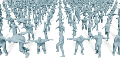
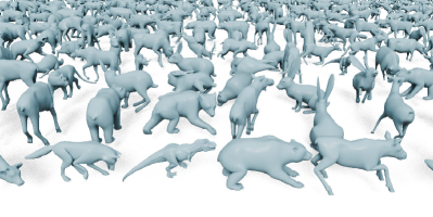
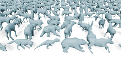
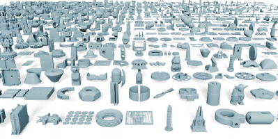
Figure 1: Our NeCGeS can compress geometry data with hundreds or even thousands of shapes into 1~2 MB while preserving details. Left: Original Geometry Data. Right: Decompressed Geometry Data.   Zoom in for details.

2 Related Work

2.1 Geometry Representation

In general, the representation of geometry data is divided into two main categories, explicit representation and implicit representation, and they could be transformed into another.

Explicit Representation. Among the explicit representations, voxelization [7] is the most intuitive. In this method, geometry models are represented by regularly distributed grids, effectively converting them into 3D ‘images’. While this approach simplifies the processing of geometry models using image processing techniques, it requires a high resolution to accurately represent the models, which demands substantial memory and limits its application. Another widely used geometry representation method is the point cloud, which consists of discrete points sampled from the surfaces of models. This method has become a predominant approach for surface representation [2, 39, 40]. However, the discrete nature of the points imposes constraints on its use in downstream tasks such as rendering and editing. Triangle meshes offer a more precise and efficient geometry representation. By approximating surfaces with numerous triangles, they achieve higher accuracy and efficiency for certain downstream tasks.

Implicit Representation. Implicit representations use the isosurface of a function or field to represent surfaces. The most widely used implicit representations include Binary Occupancy Field (BOF) [22, 35], Signed Distance Field (SDF) [36, 29], and Truncated Signed Distance Field (TSDF) [11], from which the model’s surface can be easily extracted. However, these methods are limited to representing watertight models. The Unsigned Distance Field (UDF) [8], which is the absolute value of the SDF, can represent more general models, not just watertight ones. Despite this advantage, extracting surfaces from UDF is challenging, which limits its application.

Conversion between Geometry Representations. Geometry representations can be converted between explicit and implicit forms. Various methods [21, 22, 24, 6, 35, 29, 45] are available for calculating the implicit field from given models. Conversely, when converting from implicit to explicit forms, Marching Cubes [32] and its derivatives [48, 49, 15, 45] can reconstruct continuous surfaces from various implicit fields.

2.2 3D Geometry Data Compression

Single 3D Geometric Model Compression. In recent decades, compression techniques for images and videos have rapidly advanced [51, 34, 59, 5, 4]. However, the irregular nature of geometry data makes it more challenging to compress compared to images and video, which are represented as volumetric data. A natural approach is to convert geometry data into voxelized point clouds, treating them as 3D ‘images’, and then applying image and video compression techniques to them. Following this intuition, MPEG developed the GPCC standards [13, 28, 47], where triangle meshes or triangle soup approximates the surfaces of 3D models, enabling the compression of models with more complex structures. Subsequently, several improved methods [37, 60, 53, 62] and learning-based methods [18, 43, 10, 9, 3, 42, 54] have been proposed to further enhance compression performance. However, these methods rely on voxelized point clouds to represent geometry models, which is inefficient and memory-intensive, limiting their compression efficiency. In contrast to the previously mentioned methods, Draco [12] uses a kd-tree-based coding method to compress vertices and employs the EdgeBreaker algorithm to encode the topological relationships of the geometry data. Draco utilizes uniform quantization to control the compression ratio, but its performance decreases at higher compression ratios.

Multiple Model Compression. Compared to compressing single 3D geometric models, compressing multiple objects is significantly more challenging. SLRMA [17] addresses this by using a low-rank matrix to approximate vertex matrices, thus compressing sequential models. Mekuria et al. [33] proposed the first codec for compressing sequential point clouds, where each frame is coded using Octree subdivision through an 8-bit occupancy code. Building on this concept, MPEG developed the VPCC standards [13, 28, 47], which utilize 3D-to-2D projection and encode time-varying projected planes, depth maps, and other data using video codecs. Several improved methods [57, 26, 1, 44] have been proposed to enhance the compression of sequential models. Recently, shape priors like SMPL [31] and SMAL [63] have been introduced, allowing the pose and shape of a template frame to be altered using only a few parameters. Pose-driven geometry compression methods [16, 58, 56] leverage this approach to achieve high compression efficiency. However, these methods are limited to sequences of corresponding geometry data and cannot handle sets of unrelated geometry data, which is more common in practice.

3 Proposed Method

Overview. Given a set of $N$ 3D mesh models containing diverse categories, denoted as $\mathcal{S}=\{\mathbf{S}_{i}\}_{i=1}^{N}$, we aim to compress them into a bitstream while maintaining the quality of the decompressed models as much as possible. To this end, we propose a neural compression paradigm called NeCGS. As shown in Fig. 2, NeCGS consists of two main modules, i.e., Regular Geometry Representation (RGR) and Compact Neural Representation (CNR). Specifically, RGR first represents each irregular mesh model within $\mathcal{S}$ into a regular 4D volume, namely TSDF-Def volume that mplicitly describes the geometry structure of the model, via a rendering-based optimization, thus leading to a set of 4D volumes $\mathcal{V}:=\{\mathbf{V}_{i}\}_{i=1}^{N}$ with $\mathbf{V}_{i}$ corresponding to $\mathbf{S}_{i}$. Then CNR further obtains a more compact neural representation of $\mathcal{V}$, where a quantization-aware auto-decoder-based network is constructed to regress these volumes, producing an embedded feature for each volume. Finally, the embedded features along with the network parameters are encoded into a bitstream through a typical entropy coding method to achieve compression. We also want to note that NeCGS can also be applied to compress 3D geometry sets represented in 3D point clouds, where one can either reconstruct from the given point clouds 3D surfaces through a typical surface reconstruction method or adopt a pre-trained network for SDF estimation from point clouds, e.g., SPSR [22] or IMLS [24], to bridge the gap between 3D mesh and point cloud models. In what follows, we will detail NeCGS.

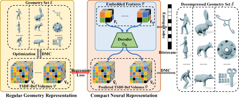
Figure 2: The pipeline of NeCGS. It first represents original meshes regularly into TSDF-Def volumes, and an auto-decoder network is utilized to regress these volume. Then the embedded features and decoder parameters are compressed into bitstreams through entropy coding. When decompressing the models, the decompressed embedded features are fed into the decoder with the decompressed parameters from the bitstreams, reconstructing the TSDF-Def volumes, and the models can be extracted from them.

3.1 Regular Geometry Representation

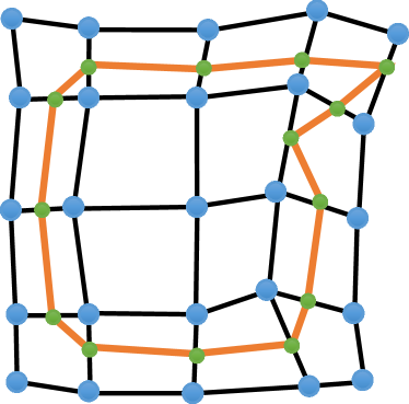
Figure 3: 2D visual illustration of DMC. The blue points refer to the deformable grid points, the green points refer to the vertices of the extracted surfaces, and the orange lines refer to the faces of the extracted surfaces. Left: The original grid points. Right: The surface extraction.

Unlike 2D images and videos, where pixels are uniformly distributed on 2D regular girds, the irregular characteristic of 3D mesh models makes it challenging to compress them efficiently and effectively. We propose to convert each 3D mesh model to a 4D regular volume called TSDF-Def volume, which implicitly represents the geometry structure of the model. Such a regular representation can describe the model precisely, and its regular nature proves beneficial for compression in the subsequent stage.

TSDF-Def Volume. Although 3D regular SDF or TSDF volumes are widely used for representing 3D geometry models, they may introduce distortions when the volume resolution is relatively limited. Inspired by recent shape extracting methods [48, 49], we propose TSDF-Def, which extends the regular TSDF volume by introducing an additional deformation for each grid point to adjust the detailed structure during the extraction of models, as shown in Fig. 3. Accordingly, we develop the differentiable Deformable Marching Cubes (DMC), the variant of the Marching Cubes method [32], for surface extraction from a TSDF-Def volume. Consequently, each shape $\mathbf{S}$ is represented as a 4D TSDF-Def volume, denoted as $\mathbf{V}\in\mathbb{R}^{\scriptscriptstyle K\times K\times K\times 4}$, where $K$ is the volume resolution. More specifically, the value of the grid point located at $(u,v,w)$ is $\mathbf{V}(u,v,w):=[\mathtt{TSDF}(u,v,w),\Delta u,\Delta v,\Delta w]$, where $(\Delta u,\Delta v,\Delta w)$ are the deformation for the grid point and $1\leq u,v,w\leq K$. TSDF-Def enhances representation accuracy, particularly when the grid resolution is relatively low.

Optimization of TSDF-Def Volumes. To obtain the optimal TSDF-Def volume $\mathbf{V}$ for a given model $\mathbf{S}$, after initializing the deformations of each grid to zero and computing the TSDF value for each grid we optimize the following problem:

$$\min_{\mathbf{V}}\mathcal{E}_{\rm Rec}(\texttt{DMC}(\mathbf{V}),\mathbf{S}),$$ (1)

where $\texttt{DMC}(\cdot)$ refers to the differentiable DMC process for extracting surfaces from TSDF-Def volumes, and the $\mathcal{E}_{\rm Reg}(\cdot,~{}\cdot)$ measures the differences between the rendered depth and silhouette images of two mesh models through the differentiable rasterization [25]. Algorithm 1 summarizes the whole optimization process. More details can be found in Sec. A.2 of the subsequent Appendix.

Input: 3D mesh model $\mathbf{S}$; the maximum number of iterations maxIter.

Output: The optimal TSDF-Def volume $\mathbf{V}\in\mathbb{R}^{\scriptscriptstyle K\times K\times K\times 4}$.

1 Place uniformly distributed grids in the cube of $\mathbf{S}$, denoted as $\mathbf{G}\in\mathbb{R}^{\scriptscriptstyle K\times K\times K\times 3}$;

2 Initialize $\mathbf{V}[...,0]$ as the ground truth TSDF of $\mathbf{S}$ at the location of $\mathbf{G}$, the deformation $\mathbf{V}[...,1:]$=0, and the current iteration $\texttt{Iter}=0$;

3 while $\mathtt{{Iter}}<\mathtt{maxIter}$ do

4       Recover shape from $\mathbf{V}$ according to DMC, $\texttt{DMC}(\mathbf{V})$;

5       Calculate the reconstruction error, $\mathcal{E}_{\text{Rec}}(\texttt{DMC}(\mathbf{V}),\mathbf{S})$;

6       Optimize $\mathbf{V}$ using ADAM optimizer based on the reconstruction error;

7       Iter:=Iter+1;

8      

9 end while

10return $\mathbf{V}$;

Algorithm 1 Optimization of TSDF-Def Volumes

3.2 Compact Neural Representation

Observing the similarity of local geometric structures within a typical 3D model and across different models, i.e., redundancy, we further propose a quantization-aware neural representation process to summarize the similarity within $\mathcal{V}$, leading to more compact representations with redundancy removed.

Network Architecture. We construct an auto-decoder network architecture to regress these 4D TSDF-Def volumes. Specifically, it is composed of a head layer, which increases the channel of its input, and $L$ cascaded upsampling modules, which progressively upscale the feature volume. We also utilize the PixelShuffle technique [50] between the convolution and activation layers to achieve upscaling. We refer reviewers to Sec. B of Appendix for more details. For TSDF-Def volume $\mathbf{V}_{i}$, the corresponding input to the auto-decoder is the embedded feature, denoted as $\mathbf{F}_{i}\in\mathbb{R}^{\scriptscriptstyle K^{\prime}\times K^{\prime}\times K^{\prime}\times C}$, where $K^{\prime}$ is the resolution satisfying $K^{\prime}\ll K$ and $C$ is the number of channels. Moreover, we integrate differentiable quantization to the embedded features and network parameters in the process, which can efficiently reduce the quantization error. In all, the compact neural representation process can be written as

$$\widehat{\mathbf{V}}_{i}=\mathcal{D}_{\mathcal{Q}(\bm{{\Theta}})}(\mathcal{Q}(\mathbf{F}_{i})).$$ (2)

where $\mathcal{Q}(\cdot)$ stands for the differentiable quantization operator, and $\widehat{\mathbf{V}}_{i}$ is the regressed TSDF-Def.

Loss Function. We employ a joint loss function comprising Mean Absolute Error (MAE) and Structural Similarity Index (SSIM) to simultaneously optimize the embedded features $\{\mathbf{F}_{i}\}$ and the network parameters $\bm{{\Theta}}$. In computing the MAE between the predicted and ground truth TSDF-Def volumes, we concentrate more on the grids close to the surface. These surface grids crucially determine the surfaces through their TSDFs and deformations; hence we assign them higher weights during optimization than the grids farther away from the surface. The overall loss function for the $i$-th model is written as

$$\mathcal{L}(\widehat{\mathbf{V}}_{i},\mathbf{V}_{i})=\|\widehat{\mathbf{V}}_{i}-\mathbf{V}_{i}\|_{1}+\lambda_{1}\|\mathbf{M}_{i}\odot(\widehat{\mathbf{V}}_{i}-\mathbf{V}_{i})\|_{1}+\lambda_{2}(1-\texttt{SSIM}(\widehat{\mathbf{V}}_{i},\mathbf{V}_{i})),$$ (3)

where $\mathbf{M}_{i}=\mathbbm{1}(|\mathbf{V}_{i}[...,0])|<\tau)$ is the mask, indicating whether a grid is near the surface, i.e., its TSDF is less than the threshold $\tau$, while $\lambda_{1}$ and $\lambda_{2}$ are the weights to balance each term of the loss function.

Entropy Coding. After obtaining the quantized features $\{\widetilde{\mathbf{F}}_{i}=\mathcal{Q}(\mathbf{F}_{i})\}$ and quantized network parameters $\widetilde{\bm{\Theta}}=\mathcal{Q}(\bm{\Theta})$, we adopt the Huffman Codec [20] to further compress them into a bitstream. More advanced entropy coding methods can be employed to further improve compression performance.

3.3 Decompression

To obtain the 3D mesh models from the bitstream, we first decompress the bitstream to derive the embedded features, $\{\widetilde{\mathbf{F}}_{i}\}$ and the decoder parameter, $\widetilde{\bm{\Theta}}$. Then, for each $\widetilde{\mathbf{F}}_{i}$, we feed it to the decoder $\mathcal{D}_{\widetilde{\bm{\Theta}}}(\cdot)$ to generate its corresponding TSDF-Def volume

$$\widehat{\mathbf{V}}_{i}=\mathcal{D}_{\widetilde{\bm{\Theta}}}(\widetilde{\mathbf{F}}_{i}).$$ (4)

Finally, we utilize DMC to recover each shape from $\widehat{\mathbf{V}}_{i}$, $\widehat{\mathbf{S}}_{i}=\texttt{DMC}(\widehat{\mathbf{V}}_{i})$, forming the set of decompressed geometry data, $\widehat{\mathcal{S}}=\{\widehat{\mathbf{S}}_{i}\}_{i=1}^{N}$.

4 Experiment

4.1 Experimental Setting

Implementation details. In the process of optimizing TSDF-Def volumes, we employed the ADAM optimizer [23] for 500 iterations per shape, using a learning rate of 0.01. The resolution of TSDF-Def volumes was $K=128$. The resolution and the number of channels of the embedded features were $K^{\prime}=4$ and $C=16$, respectively. And the decoder is composed of $L=5$ upsampling modules with an up-scaling factor of 2. During the optimization, we set $\lambda_{1}=5$ and $\lambda_{2}=10$, and the embedded features and decoder parameters were optimized by the ADAM optimizer for 400 epochs, with a learning rate of 1e-3. We achieved different compression efficiencies by adjusting decoder sizes. We conducted all experiments on an NVIDIA RTX 3090 GPU with Intel(R) Xeon(R) CPU.

Table 1: Details of the selected datasets.

Dataset	Original Size (MB)	# Models
AMA	378.41	500
DT4D	683.80	500
Thingi10K	335.92	1000
Mixed	496.16	600

Datasets. We tested our NeCGS on various types of datasets, including humans, animals, and CAD models. For human models, we randomly selected 500 shapes from the AMA dataset [52]. For animal models, we randomly selected 500 shapes from the DT4D dataset [27]. For the CAD models, we randomly selected 1000 shapes from the Thingi10K dataset [61]. Besides, we randomly selected 200 models from each dataset, forming a more challenging dataset, denoted as Mixed. The details about the selected datasets are shown in Table 1. In all experiments, we scaled all models in a cube with a range of $[-1,1]^{3}$ to ensure they are in the same scale.

Methods under Comparison. In terms of traditional geometry codecs, we chose the three most impactful geometry coding standards with released codes, G-PCC and V-PCC from MPEG (see more details about them in [13, 28, 47]), and Draco from Google as the baseline methods. Additionally, we compared our approach with state-of-the-art deep learning-based compression methods, specifically PCGCv2 [54]. Furthermore, we adapted DeepSDF [36] with quantization to serve as another baseline method, denoted as QuantDeepSDF. It is worth noting that while some of the chosen baseline methods were originally designed for point cloud compression, we utilized voxel sampling and SPSR [22] to convert them between the forms of point cloud and surface. More details can be found in Sec. C.2 appendix.

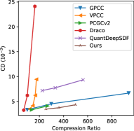
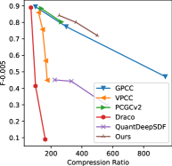
(a) AMA

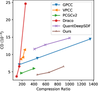
(b) DT4D

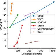
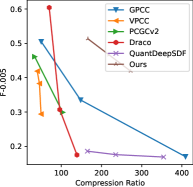
(c) Thingi10K

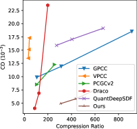
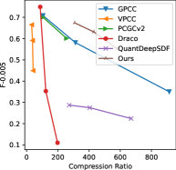
(d) Mixed

Figure 4: Quantitative comparisons of different methods on four 3D geometry sets.

Evaluation Metrics. Following previous reconstruction methods [35, 38], we utilize Chamfer Distance (CD), Normal Consistency (NC), F-Score with the thresholds of 0.005 and 0.01 (F1-0.005 and F1-0.01) as the evaluation metrics. Furthermore, to comprehensively compare the compression efficiency of different methods, we use Rate-Distortion (RD) curves. These curves illustrate the distortions at various compression ratios, with CD and F1-0.005 specifically describing the distortion of the decompressed models. Our goal is to minimize distortion, indicated by a low CD and a high F1-Score, while maximizing the compression ratio. Therefore, for the RD curve representing CD, optimal compression performance is achieved when the curve is closest to the lower right corner. Similarly, for the RD curve representing the F1-Score, the ideal compression performance is when the curve is nearest to the upper right corner. Their detailed definition can be found in Sec. C.1 of appendix.

4.2 Results

The RD curves of different compression methods under different datasets are shown in Fig. 4. As the compression ratio increases, the distortion also becomes larger. It is obvious that our NeCGS can achieve much better compression performance than the baseline methods when the compression ratio is high, even in the challenging Mixed dataset. In particular, our NeCGS achieves a minimum compression ratio of 300, and on the DT4D dataset, the compression ratio even reaches nearly 900, with minimal distortion. Due to the larger model differences within the Thingi10K and Mixed datasets compared to the other two datasets, the compression performance on these two datasets is inferior.

Figure 5: Visual comparisons of different compression methods. All numbers in corners represent the compression ratio.   Zoom in for details.

(a) Ori.

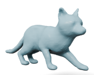
(b) 455.25

(c) 651.85

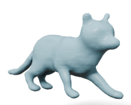
(d) 899.73

Figure 6: Decompressed models under different compression ratios.

The visual results of different compression methods are shown in Fig. 5. Compared to other methods, models compressed using our approach occupy a larger compression ratio and retain more details after decompression. Fig. 6 illustrates the decompressed models under different compression ratio. Even when the compression ratio reaches nearly 900, our method can still retain the details of the models.

4.3 Ablation Study

In order to illustrate the efficiency of each design of our NeCGS, we conducted extensive ablation study about them on the Mixed dataset.

Figure 7: Models recovered from different regular geometry representations under various volume resolutions. From Left to Right: Original, TSDF with $K=64$, TSDF with $K=128$, TSDF-Def with $K=64$, and TSDF-Def with $K=128$.

Necessity of the Deformation of Grids. We utilize TSDF-Def volumes to as the regular geometry representation, instead of TSDF volumes like previous methods. Compared with models recovered from TSDF volumes through MC, the models recovered from TSDF-Def volumes through DMC preserve more details of the thin structures, especially when the volume resolutions are relatively small, as shown in Fig. 7. We also conducted a numerical comparison of the decompressed models on the AMA dataset under these two settings, and the results are shown in Table. 2, demonstrating its advantages.

Table 2: Quantitative comparisons of different RGRs.

RGR	Size (MB)	Com. Ratio	CD ($\times 10^{-3}$) $\downarrow$	NC $\uparrow$	F1-0.005 $\uparrow$	F1-0.01 $\uparrow$
TSDF	1.631	304.20	5.015	0.944	0.662	0.936
TSDF-Def	1.612	307.79	4.913	0.947	0.674	0.943

Neural Representation Structure. To illustrate the superiority of auto-decoder framework, we utilize an auto-encoder to regress the TSDF-Def volume. Technically, we used a ConvNeXt block [30] as the encoder by replacing 2D convolutions with 3D convolutions. Under the auto-encoder framework, we optimize the parameters of the encoder to change the embedded features. The RD curves about these two structures are shown in Fig. 8, demonstrating rationality of our decoder structure.

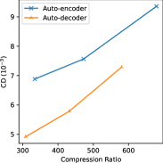
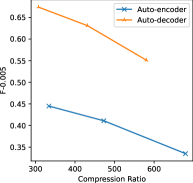
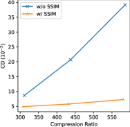
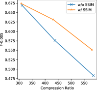
Figure 8: (a) RD curves of different neural representation structures. (b) RD curves of different regression losses.

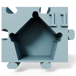
(a) Original

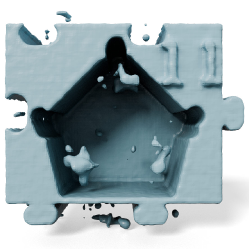
(b) w/o SSIM

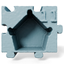
(c) w/ SSIM

Figure 9: Visual comparison of regression loss w/ and w/o SSIM item.

SSIM Loss. Compared to MAE, which focuses on one-to-one errors between predicted and ground truth volumes, the SSIM item in Eq. 3 emphasizes more on the local similarity between volumes, increasing the regression accuracy. To verify this, we removed the SSIM item and kept others unchanged. Their RD curves are shown in Fig. 8, and it is obvious that the SSIM item in the regression loss increases the compression performance. The visual comparison is shown in Fig. 9, and without SSIM, there are floating parts around the decompressed models.

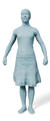
(a) Ori.

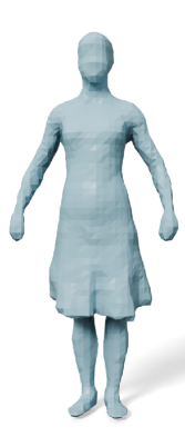
(b) 64

(c) 128

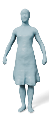
(d) 256

Figure 10: Visual comparison under different resolutions of TSDF-Def volume.

Resolution of TSDF-Def Volumes. We tested the compression performance at different resolutions of TSDF-Def volumes by adjusting the decoder layers accordingly. Specifically, we removed the last layer for a resolution of 64 and added an extra layer for a resolution of 256. The quantitative and numerical comparisons are shown in Table 3 and Fig. 10, respectively. Obviously, increasing the volume resolution can enhance the compression effectiveness, resulting in more detailed structures preserved after decompression. However, the optimization and inference time also increase accordingly due to more layers involved.

Table 3: Quantitative comparisons of different resolutions of TSDF-Def volumes.

Res.	Size (MB)	Com. Ratio	CD ($\times 10^{-3}$) $\downarrow$	NC $\uparrow$	F1-0.005 $\uparrow$	F1-0.01 $\uparrow$	Opt Time (h)	Infer. Time (ms)
64	1.408	268.75	4.271	0.927	0.721	0.966	2.16	38.97
128	1.493	253.45	3.436	0.952	0.842	0.991	16.32	98.95
256	1.627	232.58	3.234	0.962	0.870	0.995	94.50	421.94

5 Conclusion and Discussion

We have presented NeCGS, a highly effective neural compression scheme for 3D geometry sets. NeCGS has achieved remarkable compression performance on various datasets with diverse and detailed shapes, outperforming state-of-the-art compression methods to a large extent. These advantages are attributed to our regular geometry representation and the compression accomplished by a convolution-based auto-decoder. We believe our NeCGS framework will inspire further advancements in the field of geometry compression.

However, our method still suffers from the following two limitations. One is that it requires more than 15 hours to regress the TSDF-Def volumes, and the other one is that the usage of 3D convolution layers limits the inference speed. Our future work will focus on addressing these challenges by accelerating the optimization process and incorporating more efficient network modules.

Appendix

Appendix A Regular Geometry Representation

A.1 Tensor Quantization

Denoted $\mathbf{x}$ is a tensor, we quantize it in a fixed interval, $[a,b]$, at $(2^{N}+1)$ levels by

$$\mathcal{Q}(\mathbf{x})=\texttt{Round}\left(\frac{\texttt{Clamp}(\mathbf{x},a,b)-a}{s}\right)\times s+a,$$ (5)

where $s=(b-a)/2^{N}$. In our experiment, we set $a=-1$ and $b=1$.

A.2 Optimization of TSDF-deformation Volumes

We set a series of camera pose, $\mathcal{T}=\{\mathbf{T}_{i}\}_{i=1}^{E}$, around the meshes. Let $\mathbf{I}^{\scriptscriptstyle\rm{D}}_{1}(\mathbf{T}_{i})$ and $\mathbf{I}^{\scriptscriptstyle\rm{D}}_{2}(\mathbf{T}_{i})$ represent the depth images obtained from the reconstructed mesh $\texttt{DMC}(\mathbf{V})$ and the given mesh $\mathbf{S}$ at the pose $\mathbf{T}_{i}$ respectively. Similarly, let $\mathbf{I}^{\scriptscriptstyle\rm{M}}_{1}(\mathbf{T}_{i})$ and $\mathbf{I}^{\scriptscriptstyle\rm{M}}_{2}(\mathbf{T}_{i})$ denote their respective silhouette images at pose $\mathbf{T}_{i}$. The reconstruction error produced by silhouette and depth images at all pose are

$$\mathcal{E}_{\rm M}(\texttt{DMC}(\mathbf{V}),\mathbf{S})=\sum_{\mathcal{T}_{i}\in\mathcal{T}}\|\mathbf{I}^{\scriptscriptstyle\rm{M}}_{1}(\mathbf{T}_{i})-\mathbf{I}^{\scriptscriptstyle\rm{M}}_{2}(\mathbf{T}_{i})\|_{1}$$ (6)

and

$$\mathcal{E}_{\rm D}(\texttt{DMC}(\mathbf{V}),\mathbf{S})=\sum_{\mathcal{T}_{i}\in\mathcal{T}}\|\left(\mathbf{I}^{\scriptscriptstyle\rm{D}}_{1}(\mathbf{T}_{i})-\mathbf{I}^{\scriptscriptstyle\rm{D}}_{2}(\mathbf{T}_{i})\right)*\mathbf{I}^{\scriptscriptstyle\rm{M}}_{2}(\mathbf{T}_{i})\|_{1}.$$ (7)

Then the reconstruction error is defined as

$$\mathcal{E}_{\rm Rec}(\texttt{DMC}(\mathbf{V}),\mathbf{S})=\mathcal{E}_{\rm M}(\texttt{DMC}(\mathbf{V}),\mathbf{S})+\lambda_{\rm rec}\mathcal{E}_{\rm D}(\texttt{DMC}(\mathbf{V}),\mathbf{S}),$$ (8)

where $E=4$ and $\lambda_{\rm rec}=10$ in our experiment.

Appendix B Auto-decoder-based Neural Compression

B.1 Upsampling Module

In each upsampling module, we utilize a PixelShuffle layer between the convolution and activation layers to upscale the input, as shown in Fig. 11. The input feature volume has dimensions $(N_{\rm in},N_{\rm in},N_{\rm in},C_{\rm in})$, with an upsampling scale of $s$ and an output channel count of $C_{\rm out}$.

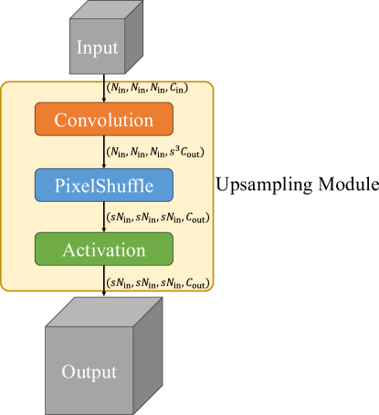
Figure 11: Upsampling Module.

Appendix C Experiment

C.1 Evaluation Metric

Let $\mathbf{S}_{\rm Rec}$ and $\mathbf{S}_{\rm GT}$ denote the reconstructed and ground-truth 3D shapes, respectively. We then randomly sample $N_{\rm eval}=10^{5}$ points on them, obtaining two point clouds, $\mathbf{P}_{\rm Rec}$ and $\mathbf{P}_{\rm GT}$. For each point of $\mathbf{P}_{\rm Rec}$ and $\mathbf{P}_{\rm GT}$, the normal of the triangle face where it is sampled is considered to be its normal vector, and the normal sets of $\mathbf{P}_{\rm Rec}$ and $\mathbf{P}_{\rm GT}$ are denoted as $\mathbf{N}_{\rm Rec}$ and $\mathbf{N}_{\rm GT}$, respectively. Let $\mathtt{NN\_Point}(\mathbf{x},\mathbf{P})$ be the operator that returns the nearest point of $\mathbf{x}$ in the point cloud $\mathbf{P}$. The CD between them is defined as

$$\texttt{CD}(\mathbf{S}_{\rm Rec},\mathbf{S}_{\rm GT})= \frac{1}{2N_{\rm eval}}\sum_{\mathbf{x}\in\mathbf{P}_{\rm Rec}}\|\mathbf{x}-\mathtt{NN\_Point}(\mathbf{x},\mathbf{P}_{\rm GT})\|_{2}$$ (9)

$$+ \frac{1}{2N_{\rm eval}}\sum_{\mathbf{x}\in\mathbf{P}_{\rm GT}}\|\mathbf{x}-\mathtt{NN\_Point}(\mathbf{x},\mathbf{P}_{\rm Rec})\|_{2}.$$

Let $\mathtt{NN\_Normal}(\mathbf{x},\mathbf{P})$ be the operator that returns the normal vector of the point $\mathbf{x}$’s nearest point in the point cloud $\mathbf{P}$. The NC is defined as

$$\texttt{NC}(\mathbf{S}_{\rm Rec},\mathbf{S}_{\rm GT})= \frac{1}{2N_{\rm eval}}\sum_{\mathbf{x}\in\mathbf{P}_{\rm Rec}}|\mathbf{N}_{\rm Rec}(\mathbf{x})\cdot\mathtt{NN\_Normal}(\mathbf{x},\mathbf{P}_{\rm GT})|$$ (10)

$$+ \frac{1}{2N_{\rm eval}}\sum_{\mathbf{x}\in\mathbf{P}_{\rm GT}}|\mathbf{N}_{\rm GT}(\mathbf{x})\cdot\mathtt{NN\_Normal}(\mathbf{x},\mathbf{P}_{\rm Rec})|.$$

F-Score is defined as the harmonic mean between the precision and the recall of points that lie within a certain distance threshold $\epsilon$ between $\mathbf{S}_{\rm Rec}$ and $\mathbf{S}_{\rm GT}$,

$$\mathtt{F-Score}(\mathbf{S}_{\rm Rec},\mathbf{S}_{\rm GT},\epsilon)=\frac{2\cdot\mathtt{Recall}\cdot\mathtt{Precision}}{\mathtt{Recall}+\mathtt{Precision}},$$ (11)

where

$$\mathtt{Recall}(\mathbf{S}_{\rm Rec},\mathbf{S}_{\rm GT},\epsilon) =\left|\left\{\mathbf{x}_{1}\in\mathbf{P}_{\rm Rec},\rm{s.t.}\min_{\mathbf{x}_{2}\in\mathbf{P}_{\rm GT}}\|\mathbf{x}_{1}-\mathbf{x}_{2}\|_{2}<\epsilon\right\}\right|,$$ (12)

$$\mathtt{Precision}(\mathbf{S}_{\rm Rec},\mathbf{S}_{\rm GT},\epsilon) =\left|\left\{\mathbf{x}_{2}\in\mathbf{P}_{\rm GT},\rm{s.t.}\min_{\mathbf{x}_{1}\in\mathbf{P}_{\rm Rec}}\|\mathbf{x}_{1}-\mathbf{x}_{2}\|_{2}<\epsilon\right\}\right|.$$

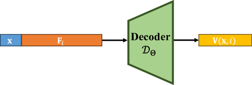
Figure 12: Pipeline of QuantDeepSDF.

C.2 QuantDeepSDF

Compared to DeepSDF, our QuantDeepSDF incorporates the following two modifications:

• The decoder parameters are quantized to enhance compression efficiency.

• To maintain consistency with our NeCGS, the points sampled during training are drawn from TSDF-Def volumes.

The pipeline of QuantDeepSDF is shown in Fig. 12. Specifically, the decoder is an MLP, where the input is the concatenated vector of coordinate $\mathbf{x}\in\mathbb{R}^{3}$ and the $i$-th embedded feature vector $\mathbf{F}_{i}\in\mathbb{R}^{C}$, and the output is the corresponding TSDF-Def value. In our experiment, the decoder consists of 8 layers, and the compression ratio is controled by changing the width of each layer.

C.3 Auto-Encoder in Ablation Study

Different from the auto-encoder used in our framework, where the embed features are directly optimized, auto-encoder utilizes an encoder to produce the embedded features, where the inputs are the TSDF-Def volumes. And the decoder is kept the same as our framework. During the optimization, the parameters of encoder and decoder are optimized. Once optimized, the embedded features produced by the encoder and decoder parameters are compressed into bitstreams.

C.4 More Visual Results

Fig. 13 depicts the visual results of the decompresed models from the AMA dataset, DT4D dataset, and Thingi10K dataset under various compression ratios, respectively. With the compression ratio increasing, the decompressed models still preserve the detailed structures, without large distortion.

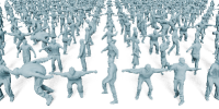
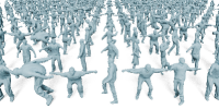
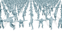
Ori.          253.45        362.80         500.54

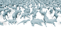
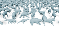
Ori.          455.26        651.85        899.73

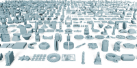
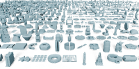
Ori.          166.79        219.84         273.32

Figure 13: Visual results of the decompressed models under different compression ratios. From Top to Bottom: AMA, DT4D, and Thingi10K.   Zoom in for details.

References

- [1] A. Ahmmed, M. Paul, M. Murshed, and D. Taubman. Dynamic point cloud geometry compression using cuboid based commonality modeling framework. In 2021 IEEE International Conference on Image Processing (ICIP), pages 2159–2163. IEEE, 2021.
- [2] P. J. Besl and N. D. McKay. Method for registration of 3-d shapes. In Sensor Fusion IV: Control Paradigms and Data Structures, volume 1611, pages 586–606. Spie, 1992.
- [3] S. Biswas, J. Liu, K. Wong, S. Wang, and R. Urtasun. Muscle: Multi sweep compression of lidar using deep entropy models. Advances in Neural Information Processing Systems, 33:22170–22181, 2020.
- [4] H. Chen, M. Gwilliam, S.-N. Lim, and A. Shrivastava. Hnerv: A hybrid neural representation for videos. In Proceedings of the IEEE/CVF Conference on Computer Vision and Pattern Recognition, pages 10270–10279, 2023.
- [5] H. Chen, B. He, H. Wang, Y. Ren, S. N. Lim, and A. Shrivastava. Nerv: Neural representations for videos. Advances in Neural Information Processing Systems, 34:21557–21568, 2021.
- [6] Z.-Q. Cheng, Y.-Z. Wang, B. Li, K. Xu, G. Dang, and S.-Y. Jin. A survey of methods for moving least squares surfaces. In Proceedings of the Fifth Eurographics/IEEE VGTC conference on Point-Based Graphics, pages 9–23, 2008.
- [7] J. Chibane, T. Alldieck, and G. Pons-Moll. Implicit functions in feature space for 3d shape reconstruction and completion. In Proceedings of the IEEE/CVF Conference on Computer Vision and Pattern Recognition, pages 6970–6981, June 2020.
- [8] J. Chibane, G. Pons-Moll, et al. Neural unsigned distance fields for implicit function learning. Advances in Neural Information Processing Systems, 33:21638–21652, 2020.
- [9] T. Fan, L. Gao, Y. Xu, D. Wang, and Z. Li. Multiscale latent-guided entropy model for lidar point cloud compression. IEEE Transactions on Circuits and Systems for Video Technology, 33(12):7857–7869, 2023.
- [10] C. Fu, G. Li, R. Song, W. Gao, and S. Liu. Octattention: Octree-based large-scale contexts model for point cloud compression. In Proceedings of the AAAI conference on artificial intelligence, volume 36, pages 625–633, 2022.
- [11] P. Gao, Z. Jiang, H. You, P. Lu, S. C. Hoi, X. Wang, and H. Li. Dynamic fusion with intra-and inter-modality attention flow for visual question answering. In Proceedings of the IEEE/CVF conference on computer vision and pattern recognition, pages 6639–6648, 2019.
- [12] Google. Point cloud compression reference software. Website. https://github. com/google/draco.
- [13] D. Graziosi, O. Nakagami, S. Kuma, A. Zaghetto, T. Suzuki, and A. Tabatabai. An overview of ongoing point cloud compression standardization activities: Video-based (v-pcc) and geometry-based (g-pcc). APSIPA Transactions on Signal and Information Processing, 9:e13, 2020.
- [14] A. F. Guarda, N. M. Rodrigues, and F. Pereira. Point cloud coding: Adopting a deep learning-based approach. In 2019 Picture Coding Symposium (PCS), pages 1–5. IEEE, 2019.
- [15] B. Guillard, F. Stella, and P. Fua. Meshudf: Fast and differentiable meshing of unsigned distance field networks. In European Conference on Computer Vision, pages 576–592, 2022.
- [16] J. Hou, L.-P. Chau, N. Magnenat-Thalmann, and Y. He. Compressing 3-d human motions via keyframe-based geometry videos. IEEE Transactions on Circuits and Systems for Video Technology, 25(1):51–62, 2014.
- [17] J. Hou, L.-P. Chau, N. Magnenat-Thalmann, and Y. He. Sparse low-rank matrix approximation for data compression. IEEE Transactions on Circuits and Systems for Video Technology, 27(5):1043–1054, 2015.
- [18] L. Huang, S. Wang, K. Wong, J. Liu, and R. Urtasun. Octsqueeze: Octree-structured entropy model for lidar compression. In Proceedings of the IEEE/CVF conference on computer vision and pattern recognition, pages 1313–1323, 2020.
- [19] T. Huang and Y. Liu. 3d point cloud geometry compression on deep learning. In Proceedings of the 27th ACM international conference on multimedia, pages 890–898, 2019.
- [20] D. A. Huffman. A method for the construction of minimum-redundancy codes. Proceedings of the IRE, 40(9):1098–1101, 1952.
- [21] M. Kazhdan, M. Bolitho, and H. Hoppe. Poisson surface reconstruction. In Proceedings of the fourth Eurographics symposium on Geometry processing, pages 61–70, 2006.
- [22] M. Kazhdan and H. Hoppe. Screened poisson surface reconstruction. ACM Transactions on Graphics (ToG), 32(3):1–13, 2013.
- [23] D. P. Kingma and J. Ba. Adam: A method for stochastic optimization. arXiv preprint arXiv:1412.6980, 2014.
- [24] R. Kolluri. Provably good moving least squares. ACM Transactions on Algorithms, 4(2):1–25, 2008.
- [25] S. Laine, J. Hellsten, T. Karras, Y. Seol, J. Lehtinen, and T. Aila. Modular primitives for high-performance differentiable rendering. ACM Transactions on Graphics (ToG), 39(6):1–14, 2020.
- [26] L. Li, Z. Li, V. Zakharchenko, J. Chen, and H. Li. Advanced 3d motion prediction for video-based dynamic point cloud compression. IEEE Transactions on Image Processing, 29:289–302, 2019.
- [27] Y. Li, H. Takehara, T. Taketomi, B. Zheng, and M. Nießner. 4dcomplete: Non-rigid motion estimation beyond the observable surface. In Proceedings of the IEEE/CVF International Conference on Computer Vision, pages 12706–12716, 2021.
- [28] H. Liu, H. Yuan, Q. Liu, J. Hou, and J. Liu. A comprehensive study and comparison of core technologies for mpeg 3-d point cloud compression. IEEE Transactions on Broadcasting, 66(3):701–717, 2019.
- [29] S.-L. Liu, H.-X. Guo, H. Pan, P.-S. Wang, X. Tong, and Y. Liu. Deep implicit moving least-squares functions for 3d reconstruction. In Proceedings of the IEEE/CVF Conference on Computer Vision and Pattern Recognition, pages 1788–1797, June 2021.
- [30] Z. Liu, H. Mao, C.-Y. Wu, C. Feichtenhofer, T. Darrell, and S. Xie. A convnet for the 2020s. In Proceedings of the IEEE/CVF conference on computer vision and pattern recognition, pages 11976–11986, 2022.
- [31] M. Loper, N. Mahmood, J. Romero, G. Pons-Moll, and M. J. Black. Smpl: A skinned multi-person linear model. ACM Trans. Graph., 34(6), oct 2015.
- [32] W. E. Lorensen and H. E. Cline. Marching cubes: A high resolution 3d surface construction algorithm. ACM siggraph computer graphics, 21(4):163–169, 1987.
- [33] R. Mekuria, K. Blom, and P. Cesar. Design, implementation, and evaluation of a point cloud codec for tele-immersive video. IEEE Transactions on Circuits and Systems for Video Technology, 27(4):828–842, 2016.
- [34] F. Mentzer, E. Agustsson, M. Tschannen, R. Timofte, and L. V. Gool. Practical full resolution learned lossless image compression. In Proceedings of the IEEE/CVF conference on computer vision and pattern recognition, pages 10629–10638, 2019.
- [35] L. Mescheder, M. Oechsle, M. Niemeyer, S. Nowozin, and A. Geiger. Occupancy networks: Learning 3d reconstruction in function space. In Proceedings of the IEEE/CVF Conference on Computer Vision and Pattern Recognition, pages 4460–4470, June 2019.
- [36] J. J. Park, P. Florence, J. Straub, R. Newcombe, and S. Lovegrove. Deepsdf: Learning continuous signed distance functions for shape representation. In Proceedings of the IEEE/CVF Conference on Computer Vision and Pattern Recognition, pages 165–174, June 2019.
- [37] E. Peixoto. Intra-frame compression of point cloud geometry using dyadic decomposition. IEEE Signal Processing Letters, 27:246–250, 2020.
- [38] S. Peng, M. Niemeyer, L. Mescheder, M. Pollefeys, and A. Geiger. Convolutional occupancy networks. In European Conference on Computer Vision, pages 523–540. Springer, 2020.
- [39] C. R. Qi, H. Su, K. Mo, and L. J. Guibas. Pointnet: Deep learning on point sets for 3d classification and segmentation. In Proceedings of the IEEE Conference on Computer Vision and Pattern Recognition, pages 652–660, 2017.
- [40] C. R. Qi, L. Yi, H. Su, and L. J. Guibas. Pointnet++: Deep hierarchical feature learning on point sets in a metric space. Advances in neural information processing systems, 30:1–xxx, 2017.
- [41] M. Quach, G. Valenzise, and F. Dufaux. Learning convolutional transforms for lossy point cloud geometry compression. In 2019 IEEE international conference on image processing (ICIP), pages 4320–4324. IEEE, 2019.
- [42] M. Quach, G. Valenzise, and F. Dufaux. Learning convolutional transforms for lossy point cloud geometry compression. In 2019 IEEE international conference on image processing (ICIP), pages 4320–4324. IEEE, 2019.
- [43] Z. Que, G. Lu, and D. Xu. Voxelcontext-net: An octree based framework for point cloud compression. In Proceedings of the IEEE/CVF Conference on Computer Vision and Pattern Recognition, pages 6042–6051, 2021.
- [44] E. Ramalho, E. Peixoto, and E. Medeiros. Silhouette 4d with context selection: Lossless geometry compression of dynamic point clouds. IEEE Signal Processing Letters, 28:1660–1664, 2021.
- [45] S. Ren, J. Hou, X. Chen, Y. He, and W. Wang. Geoudf: Surface reconstruction from 3d point clouds via geometry-guided distance representation. In Proceedings of the IEEE/CVF Internation Conference on Computer Vision, pages 14214–14224, 2023.
- [46] S. Schwarz, M. Preda, V. Baroncini, M. Budagavi, P. Cesar, P. A. Chou, R. A. Cohen, M. Krivokuća, S. Lasserre, Z. Li, et al. Emerging mpeg standards for point cloud compression. IEEE Journal on Emerging and Selected Topics in Circuits and Systems, 9(1):133–148, 2018.
- [47] S. Schwarz, M. Preda, V. Baroncini, M. Budagavi, P. Cesar, P. A. Chou, R. A. Cohen, M. Krivokuća, S. Lasserre, Z. Li, et al. Emerging mpeg standards for point cloud compression. IEEE Journal on Emerging and Selected Topics in Circuits and Systems, 9(1):133–148, 2018.
- [48] T. Shen, J. Gao, K. Yin, M.-Y. Liu, and S. Fidler. Deep marching tetrahedra: a hybrid representation for high-resolution 3d shape synthesis. Advances in Neural Information Processing Systems, 34:6087–6101, 2021.
- [49] T. Shen, J. Munkberg, J. Hasselgren, K. Yin, Z. Wang, W. Chen, Z. Gojcic, S. Fidler, N. Sharp, and J. Gao. Flexible isosurface extraction for gradient-based mesh optimization. ACM Transactions on Graphics (TOG), 42(4):1–16, 2023.
- [50] W. Shi, J. Caballero, F. Huszár, J. Totz, A. P. Aitken, R. Bishop, D. Rueckert, and Z. Wang. Real-time single image and video super-resolution using an efficient sub-pixel convolutional neural network. In Proceedings of the IEEE conference on computer vision and pattern recognition, pages 1874–1883, 2016.
- [51] Y. Strümpler, J. Postels, R. Yang, L. V. Gool, and F. Tombari. Implicit neural representations for image compression. In European Conference on Computer Vision, pages 74–91. Springer, 2022.
- [52] D. Vlasic, I. Baran, W. Matusik, and J. Popović. Articulated mesh animation from multi-view silhouettes. ACM Transactions on Graphics, 27(3):1–9, 2008.
- [53] C. Wang, W. Zhu, Y. Xu, Y. Xu, and L. Yang. Point-voting based point cloud geometry compression. In 2021 IEEE 23rd International Workshop on Multimedia Signal Processing (MMSP), pages 1–5. IEEE, 2021.
- [54] J. Wang, D. Ding, Z. Li, and Z. Ma. Multiscale point cloud geometry compression. In 2021 Data Compression Conference (DCC), pages 73–82. IEEE, 2021.
- [55] J. Wang, H. Zhu, H. Liu, and Z. Ma. Lossy point cloud geometry compression via end-to-end learning. IEEE Transactions on Circuits and Systems for Video Technology, 31(12):4909–4923, 2021.
- [56] X. Wu, P. Zhang, M. Wang, P. Chen, S. Wang, and S. Kwong. Geometric prior based deep human point cloud geometry compression. IEEE Transactions on Circuits and Systems for Video Technology, 2024.
- [57] J. Xiong, H. Gao, M. Wang, H. Li, K. N. Ngan, and W. Lin. Efficient geometry surface coding in v-pcc. IEEE Transactions on Multimedia, 25:3329–3342, 2022.
- [58] R. Yan, Q. Yin, X. Zhang, Q. Zhang, G. Zhang, and S. Ma. Pose-driven compression for dynamic 3d human via human prior models. IEEE Transactions on Pattern Analysis and Machine Intelligence, 2024.
- [59] Y. Yang, R. Bamler, and S. Mandt. Improving inference for neural image compression. Advances in Neural Information Processing Systems, 33:573–584, 2020.
- [60] X. Zhang, W. Gao, and S. Liu. Implicit geometry partition for point cloud compression. In 2020 Data Compression Conference (DCC), pages 73–82. IEEE, 2020.
- [61] Q. Zhou and A. Jacobson. Thingi10k: A dataset of 10,000 3d-printing models. arXiv preprint arXiv:1605.04797, 2016.
- [62] W. Zhu, Y. Xu, D. Ding, Z. Ma, and M. Nilsson. Lossy point cloud geometry compression via region-wise processing. IEEE Transactions on Circuits and Systems for Video Technology, 31(12):4575–4589, 2021.
- [63] S. Zuffi, A. Kanazawa, D. Jacobs, and M. J. Black. 3D menagerie: Modeling the 3D shape and pose of animals. In IEEE Conf. on Computer Vision and Pattern Recognition (CVPR), July 2017.