Generation of vortex electrons by atomic photoionization

I. I. Pavlov ilya.pavlov@metalab.ifmo.ru School of Physics and Engineering, ITMO University, 197101 St. Petersburg, Russia    A. D. Chaikovskaia alisa.katanaeva@metalab.ifmo.ru School of Physics and Engineering, ITMO University, 197101 St. Petersburg, Russia    D. V. Karlovets dmitry.karlovets@metalab.ifmo.ru School of Physics and Engineering, ITMO University, 197101 St. Petersburg, Russia
Abstract

We explore the process of orbital angular momentum (OAM) transfer from a twisted light beam to an electron in atomic ionization within the first Born approximation. The characteristics of the ejected electron are studied regardless of the detection scheme. We find that the outgoing electron possesses a definite projection of OAM when a single atom is located on the propagation axis of the photon, whereas the size of the electron wave packet is solely determined by the energy of the photon rather than by its transverse coherence length. Shifting the position of the atom yields a finite dispersion of the electron OAM. We also study a more experimentally feasible scenario — a localized finite-sized atomic target — and develop representative approaches to describing coherent and incoherent regimes of photoionization.

Introduction. Atomic photoionization by twisted light was under investigation in several recent papers [1, 2, 3, 4, 5, 6], with the focus staying on the process cross-section and the angular distribution of photoelectrons. However, there is a fundamental issue that was not directly addressed. 
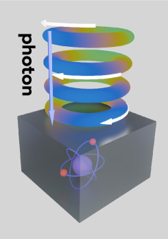
In this Letter, we theoretically demonstrate the principal possibility to generate twisted photoelectrons by using the twisted laser beam, i.e. photons carrying quanta of orbital angular momentum (OAM). We explore the resulting quantum state of the electron in the photoionization process, the stages of which are depicted in Fig. 1, and regardless of the detection protocol. Particular attention is given to the OAM transfer from the incident photon to the photoelectron. The incident vortex photon is taken in the form of a Bessel beam [7] and a Laguerre-Gaussian wave packet [8], while for the target ”cathode” there are also two toy-model options: a single (hydrogen) atom in 1s1𝑠1s state and a finite target consisting of symmetrically spread single atoms.

Photoemission of vortex electrons is a first step in one of the approaches towards generating relativistic electron beams with OAM at particle accelerators. Specifically, it is an ongoing experimental joint ITMO-JINR project on relativistic vortex electron generation at Dzhelepov Laboratory of Nuclear Problems of JINR [9] that can benefit from this study. Relativistic beams of electrons, protons and other charged particles with OAM can become a unique research tool not only in atomic and molecular physics, in the diagnostics of nanomaterials and surfaces, where the orbital momentum allows one to obtain new information about a sample, but also in nuclear physics, spin and hadron physics, where such particles can be used to analyze the proton spin, study nuclear forces at low energies, etc [10, 11, 12, 13, 14].

In the straightforward theoretical approach111Natural system of units is used throughout the paper with $\hbar=c=1$ whereas the electron mass and charge are denoted as $m$ and $e<0$, respectively. to photoionization one takes the $S$-matrix element in the first order of perturbation theory [15], which describes the transition between initial (bound) and final (continuum) electron states and contains the energy conservation law:

$$S_{fi}=2\pi i\delta(\varepsilon_{i}+\omega-\varepsilon_{f})M_{fi},$$ (1)

where $\varepsilon_{i}$, $\varepsilon_{f}$ and $\omega$ are the energies of the bound state, continuum state and the photon, respectively. The transition amplitude $M_{fi}$ can be taken in the non-relativistic form as the energy of the final electron cannot exceed that of the photon, which typically varies from $10$ eV to $100$ eV (optical and ultraviolet range):

$$M_{fi}=-i\frac{e}{m}\int\psi_{f}^{*}(\bm{r})\bm{A}(\bm{r})\cdot\bm{\nabla}\psi_{i}(\bm{r})\ \differential^{3}\bm{r}$$ (2)

with $\psi_{i}(\bm{r})$ and $\psi_{f}(\bm{r})$ being the scalar wave functions, and $\bm{A}$ – the vector potential of a photon. Employing the first Born approximation is the next obvious step when energies $\omega$ are well above the $1s$ ionization threshold (as is the case with $\varepsilon_{i}=-1\operatorname{Ry}=-me^{4}/2\approx-13.6$ eV for the hydrogen atom). Then, the outgoing electron is described with an asymptotic state with a well-defined momentum, i.e. a plane wave, and such approach has been successfully applied to describe the ionization by vortex light beams in Refs. [1, 2, 3, 4]. A more complex method accounts for the modulation of a free-electron state with the incident laser field by taking the emerging electron wave function in the form of the Volkov-type solution (the so-called Keldysh photoionization theory) [16, 17, 18, 19].

Refer to caption
Refer to caption
Refer to caption
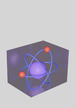
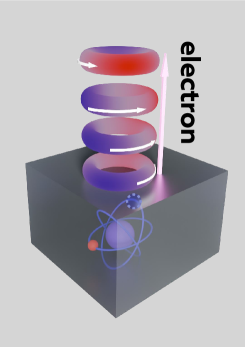
Figure 1: Photoionization of atomic target in three stages: left, twisted light beam descends onto the cathode; central, the atom(s) in the cathode become excited; right, a twisted photoelectron is emitted. A cathode, treated as a target in the scattering process, can be a single atom or an atomic ensemble.

A different approach to this problem is to consider the so-called evolved state amplitude, without making projections onto the specific basis [20, 21]. One can also mention a nonperturbative approach based on numerical solution of the exact time-dependent Schrödinger equation, which enables to track the temporal dynamics of the electron without specifying the form of its final state [22, 23, 24].

We aim to develop a measurement-strategy independent approach, which – on the one hand – allows one to deduce the quantum state of the outgoing photoelectron as it evolves from the process on its own, and – on the other hand – involves well-known perturbative calculations rather than complex numerical simulations.

We use the aforementioned evolved state formalism [20, 21] to derive the wave function of a final photoelectron independently of the post-selection protocol chosen for it, but taking into account full information on the interaction itself and the initial state of the system. Let us call the bound state of the electron $\ket{i}$, then, the evolved (pre-selected) state $\ket{\text{ev}}$ is connected to it via the $S$-matrix $\hat{S}$. Inserting a complete set of the free electron states in the form of plane waves we obtain the expression

$$\ket{\text{ev}}=\hat{S}\ket{i}=\int\frac{\differential^{3}p_{f}}{(2\pi)^{3}}\ket{\bm{p}_{f}}S_{fi}(\bm{p}_{f}).$$ (3)

Projection onto a state with a definite momentum $\ket{\bm{p}}$ yields the final state wave function in the momentum representation:

$\displaystyle\psi_{\text{ev}}(\bm{p})\equiv\innerproduct{\bm{p}}{\text{ev}}=\int\frac{\differential^{3}p_{f}}{(2\pi)^{3}}\innerproduct{\bm{p}}{\bm{p}_{f}}S_{fi}(\bm{p}_{f})$
$\displaystyle=\int\differential^{3}p_{f}\delta(\bm{p}-\bm{p}_{f})S_{fi}(\bm{p}_{f})=S_{fi}(\bm{p}).$ (4)

Thus, the wave function of the evolved state in momentum representation simply coincides with the S-matrix element. The importance of the S-matrix element phase, $\text{arg}\,S_{fi}$, is showcased in this approach, as the processes in particle physics are commonly described with only the absolute value, $|S_{fi}|$.

Since we describe the electron with the Schrödinger equation and do not take its spin into account, the OAM of the electron coincides with its total angular momentum (TAM). The OAM projection operator in the momentum representation acts as follows

$$\bra{\bm{p}}\hat{L}_{z}\ket{\text{ev}}=-i\partialderivative{\varphi_{p}}\innerproduct{\bm{p}}{\text{ev}}.$$ (5)

First, we reproduce the result for the amplitude (2) in the scenario with the incident photon being a plane wave with momentum ${\bf k}=(\bm{k}_{\perp},k_{z})=\omega(\sin{\theta_{k}}\cos{\varphi_{k}},\sin{\theta_{k}}\sin{\varphi_{k}},\cos{\theta_{k}})$ and helicity $\Lambda=\pm 1$, it is also convenient to take the Coulomb gauge

$$A=(0,\bm{A}_{\bm{k}\Lambda}(\bm{r})),\ \bm{A}_{\bm{k}\Lambda}(\bm{r})=\bm{e}_{\bm{k}\Lambda}e^{i\bm{kr}}.$$ (6)

From hereon we assume the initial electron to be described by the ground state wave function of the “hydrogen” atom with charge $Ze$ [15]: $\psi_{i}(\bm{r})=Z^{3/2}e^{-Zr/a}/\sqrt{\pi a^{3}},$ where $a=1/(me^{2})$ is the Bohr radius. The asymptotics of the complete basis of the final electron states can be chosen as plane waves: $\psi_{f}(\bm{r})=e^{i\bm{p}\bm{r}},\;\bm{p}=(\bm{p}_{\perp},p_{z})=p(\sin{\theta_{p}}\cos{\varphi_{p}},\sin{\theta_{p}}\sin{\varphi_{p}},\cos{\theta_{p}}).$ This constitutes the first Born approximation, in which one neglects the interaction of the final electron with the laser field and the electron–ion attraction after the ionization process. In other words, the electron is assumed to be emitted into the free space. The plane wave amplitude then becomes [1]

$$M_{fi}=\mathcal{N}p\frac{\bm{n}\bm{e}_{\bm{k}\Lambda}}{\left(\frac{Z^{2}}{a^{2}}+q^{2}\right)^{2}},$$ (7)

where $\mathcal{N}=-\frac{8e}{m}\sqrt{\frac{Z^{5}\pi}{a^{5}}}$, $\bm{n}=\bm{p}/p$ and $\bm{q}=\bm{p}-\bm{k}$ is the transferred momentum.

A Bessel beam. When the incoming photon is in a twisted state, a single plane wave is replaced by a superposition of plane waves. Let us consider a Bessel beam and also introduce the possible impact parameter $\bm{b}$:

$\displaystyle\bm{A}_{\kappa\ell k_{z}\Lambda}(\bm{r})$ $\displaystyle=\int\frac{\differential^{2}k_{\perp}}{(2\pi)^{2}}a_{\kappa\ell}(\bm{k}_{\perp})\bm{A}_{\bm{k}\Lambda}(\bm{r})e^{-i\bm{k}_{\perp}\bm{b}},$ (8)
$\displaystyle a_{\kappa\ell}(\bm{k}_{\perp})$ $\displaystyle=\sqrt{\frac{2\pi}{\kappa}}(-i)^{\ell}e^{i\ell\varphi_{k}}\delta(\absolutevalue{\bm{k}_{\perp}}-\kappa)$ (9)

with $\kappa$ being the absolute value of the transverse momentum and $\ell=0,\pm 1,\pm 2,\dots$ being the $z$-projection of the TAM. The amplitude, and correspondingly the evolved wave function is obtained through the integration of the plane wave amplitude (7) with the same weights as in Eq. (8). Then, the amplitude for ionization by the Bessel beam representing the process from Fig. 1 is

$\displaystyle M_{fi}^{\text{\text{TW}}}=\int\frac{\differential^{2}k_{\perp}}{(2\pi)^{2}}a_{\kappa\ell}(\bm{k}_{\perp})e^{-i\bm{k}_{\perp}\bm{b}}(\bm{k}_{\perp})M_{fi}$ (10)
$\displaystyle=\mathcal{N}p\sqrt{\frac{\kappa}{2\pi}}(-i)^{\ell}\int\frac{\differential\varphi_{k}}{2\pi}e^{i\ell\varphi_{k}-i\kappa b\cos(\varphi_{k}-\varphi_{b})}\frac{\bm{n}\bm{e}_{\bm{k}\Lambda}}{\left(\frac{Z^{2}}{a^{2}}+q^{2}\right)^{2}}.$

Introducing $\tilde{\varphi}\equiv\varphi_{k}-\varphi_{p}$ and rewriting $\frac{Z^{2}}{a^{2}}+q^{2}=\alpha-\beta\cos{\tilde{\varphi}}$ in terms of the variables $\alpha\equiv\frac{Z^{2}}{a^{2}}+p^{2}+k^{2}-2p_{z}k_{z}$ and $\beta\equiv 2p_{\perp}k_{\perp}$ allows us to put the amplitude as follows:

$\displaystyle M_{fi}^{\text{TW}}=\mathcal{N}\sqrt{\frac{\kappa}{2\pi}}(-i)^{\ell}e^{i\ell\varphi_{p}}\Bigg{\{}\frac{p_{\perp}}{\sqrt{2}}\Big{[}d_{-1\Lambda}^{1}I_{\ell+1}(\alpha,\beta,\bm{b},\varphi_{p})$
$\displaystyle-d_{1\Lambda}^{1}I_{\ell-1}(\alpha,\beta,\bm{b},\varphi_{p})\Big{]}+p_{z}d_{0\Lambda}^{1}I_{\ell}(\alpha,\beta,\bm{b},\varphi_{p})\Bigg{\}},$ (11)

where $d^{J}_{MM^{\prime}}$ are the small Wigner matrices (see details in Appendix A), and we define the function

$$I_{\ell}(\alpha,\beta,\bm{b},\varphi_{p})\equiv\int\frac{\differential\tilde{\varphi}}{2\pi}e^{i\ell\tilde{\varphi}-i\kappa b\cos(\tilde{\varphi}+\varphi_{p}-\varphi_{b})}\frac{1}{(\alpha-\beta\cos{\tilde{\varphi}})^{2}}.$$ (12)

In fact, we can make an immediate conclusion about the evolved state of the photoelectron when the ionizing beam falls onto the target atom with a vanishing impact parameter. If $\bm{b}=0$, $I_{\ell}(\alpha,\beta,0)$ does not depend on $\varphi_{p}$. Thus,

$$-i\partialderivative{\varphi_{p}}M_{fi}^{\text{TW}}=\ell M_{fi}^{\text{TW}},$$ (13)

leading to $-i\partialderivative{\varphi_{p}}S_{fi}^{\text{TW}}=\ell S_{fi}^{\text{TW}}$ and, consequently,

$$\hat{L}_{z}\ket{\text{ev}}=\ell\ket{\text{ev}}.$$ (14)

This equation illustrates that the evolved state represents a vortex electron with the OAM $z$-projection equal to $\ell$. A similar result can be expected for the ionization of some excited state of the hydrogen-like atom with a well-defined OAM projection $\ell_{e}$ onto the $z$ axis, as the conservation of the OAM projection is a consequence of the system being axially symmetric. In this case the electron OAM would clearly become $\ell+\ell_{e}$.

Moreover, in this case the amplitude can be evaluated analytically as [25, 26]

$$I_{\ell}(\alpha,\beta,0)=-\partialderivative{\alpha}\left\{\left(\frac{\beta}{\alpha+\sqrt{\alpha^{2}-\beta^{2}}}\right)^{|\ell|}\frac{1}{\sqrt{\alpha^{2}-\beta^{2}}}\right\}.$$ (15)

For a non-vanishing impact parameter, we make an estimation supposing that $\kappa b$ is a reasonable small parameter in our problem. For realistic wavelengths of the laser field $\lambda\sim 10^{2}-10^{3}$ nm and the Bessel beam opening angle $\theta_{k}\sim 1^{\circ}$ it means that we consider values $b\ll 1-10$ $\mu$m, which are relevant to the beam axis positioning accuracy in experiments with trapped atoms [27, 28, 29]. Expansion of the impact parameter - dependent exponent in (12) up to the linear term:

$\displaystyle e^{-i\kappa b\cos(\tilde{\varphi}+\varphi_{p}-\varphi_{b})}\approx$ $\displaystyle 1-\frac{i\kappa b}{2}e^{-i\varphi_{b}}e^{i(\tilde{\varphi}+\varphi_{p})}$ (16)
$\displaystyle-\frac{i\kappa b}{2}e^{i\varphi_{b}}e^{-i(\tilde{\varphi}+\varphi_{p})}$

is equivalent to making the following replacement in Eq. (11):

$\displaystyle I_{\ell}(\alpha,\beta,\bm{b})\rightarrow$ $\displaystyle I_{n}(\alpha,\beta,0)-\frac{i\kappa b}{2}e^{-i\varphi_{b}}e^{i\varphi_{p}}I_{\ell+1}(\alpha,\beta,0)$ (17)
$\displaystyle-\frac{i\kappa b}{2}e^{i\varphi_{b}}e^{-i\varphi_{p}}I_{\ell-1}(\alpha,\beta,0).$

We see that in this case the evolved state is a superposition of the twisted states with OAM values $l$ and $l\pm 1$ rather then an eigenstate of $\hat{L}_{z}$. Analogously, the expansion of exponent up to the arbitrary $n$-th term gives rise to the new terms in the superposition with OAM $l\pm n$. The coefficients at these terms are suppressed by the factor of $(\kappa b)^{n}$. The fact that in this case the photoelectron no longer represents a single twisted state is of no surprise since displacement of the target atom with respect to center of the wavefront breaks the cylindrical symmetry of the overall system.

A Laguerre-Gaussian beam. Let us now consider a more realistic model of a twisted photon beam, represented by a Laguerre-Gaussian (LG) wave packet. The vector potential is taken in the form

$$\bm{A}(\bm{r})=\bm{e}_{\Lambda}u(\bm{r})e^{ikz},$$ (18)

where the polarization vector $\bm{e}_{\Lambda}$ is supposed to be orthogonal to the $z$ axis and the scalar amplitude $u(\bm{r})$ satisfies the paraxial Helmholtz equation [30]. For the LG beam it is chosen as [8]

$\displaystyle u\left(r_{\perp},\phi,z\right)=\frac{1}{w(z)}\left(\frac{\sqrt{2}r_{\perp}}{w(z)}\right)^{\ell}$ (19)
$\displaystyle\times\exp\left[-\frac{r_{\perp}^{2}}{w^{2}(z)}\right]L_{p}^{\ell}\left(\frac{2r_{\perp}^{2}}{w^{2}(z)}\right)$
$\displaystyle\times\exp\left[i\ell\varphi+\frac{ikr_{\perp}^{2}z}{2\left(z^{2}+z_{R}^{2}\right)}-i(2p+\ell+1)\arctan\left(\frac{z}{z_{R}}\right)\right].$

The beam is monochromatic and its TAM projection is $l+\Lambda$. The atom is supposed to lie at the beam focus ($z=0$), so we can focus on the modifications in the transverse plane. There, the LG profile has a characteristic ringlike pattern with a finite number of rings determined by the radial index $p$ in contrast to Bessel beams with an infinite number of rings.

Refer to caption

(a)

Refer to caption

(b)

Refer to caption

(c)

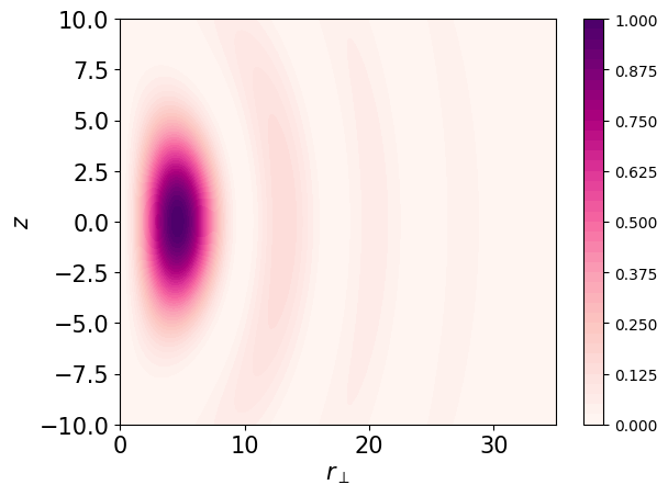
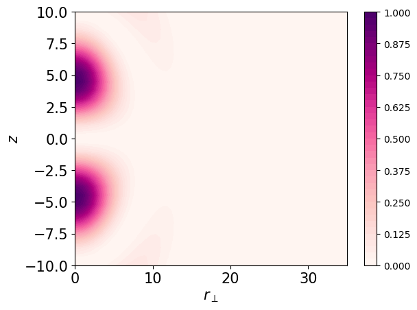
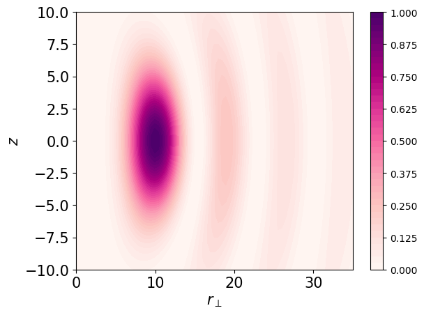
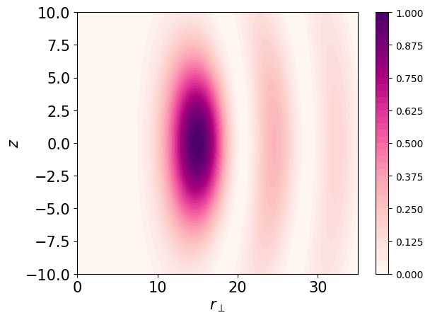
Figure 2: Normalized probability density $|\psi_{\text{ev}}(r_{\perp},z,\varphi=0)|^{2}$ of the evolved state. Due to the azimuthal symmetry of the problem there is no dependence on $\varphi$. The incident photon represents Bessel beam with $\omega=1.2|\varepsilon_{i}|$, opening angle $\theta_{k}=\arctan(\kappa/k_{z})=1^{\circ}$. Length is measured in Bohr radii $a$. (a) $\ell=0$; (b) $\ell=1$; (c) $\ell=5$.
Refer to caption

(a)

Refer to caption

(b)

Refer to caption

(c)

Refer to caption

(c)

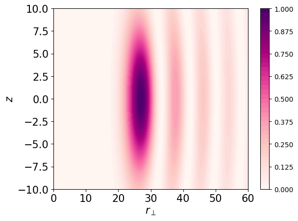
Figure 3: The same as in Fig. 2, but for the incident Laguerre-Gaussian beam with $\omega=1.2|\varepsilon_{i}|$, $w_{0}=0.5$ mm. (a) $l=p=0$ (Gaussian beam); (b) $\ell=3,p=1$; c) $\ell=5,p=3$; (d) $\ell=10,p=3$.

It is convenient to also represent the LG beam as a superposition of plane waves:

$$\bm{A}(\bm{r})=\int\frac{\differential^{2}k_{\perp}}{(2\pi)^{2}}U(\bm{k}_{\perp})\bm{e}_{\Lambda}e^{i\bm{k}\bm{r}}$$ (20)

The modulus of the wave vector is kept fixed: $k=\sqrt{k_{z}^{2}+k_{\perp}^{2}}=\operatorname{const}$. The function $U(\bm{k}_{\perp})$ is connected to the amplitude $u(\bm{r})$ in the beam focus by the two-dimensional Fourier transform:

$\displaystyle U(\bm{k}_{\perp})=$ $\displaystyle\displaystyle\int u(r_{\perp},\varphi,z=0)e^{-i\bm{k}_{\perp}\bm{r}_{\perp}}\differential^{2}r_{\perp},$ (21)
$\displaystyle U(\bm{k}_{\perp})=$ $\displaystyle\pi(-1)^{p}2^{-l/2}i^{-\ell}w_{0}^{\ell+1}k_{\perp}^{\ell}\exp\left[-\frac{k_{\perp}^{2}w_{0}^{2}}{4}\right]$ (22)
$\displaystyle\times L_{p}^{\ell}\left(\frac{k_{\perp}^{2}w_{0}^{2}}{2}\right)\exp\left[i\ell\varphi_{k}\right],$

where the beam waist $w_{0}\equiv w(z=0)$. However, such a vector potential does not satisfy Coulomb gauge, because the superposition contains nontransverse plane waves. To fix this, we make the following modification of the vector potential (see details in [31]):

$$\bm{A}_{\text{trans}}(\bm{r})=\int\frac{\differential^{2}k_{\perp}}{(2\pi)^{2}}U(\bm{k}_{\perp})e^{i\Lambda\varphi_{k}}\bm{e}_{\bm{k}\Lambda}e^{i\bm{k}\bm{r}}$$ (23)

with the polarization vector defined in Eq. (37). Interestingly, a similar issue on the ambiguity of the phase factor in the twisted wave function was discussed in [21]).

Analogously to Eq. (10), the amplitude of the photoionization process with an incident LG beam is given by

$\displaystyle M_{fi}^{LG}=$ $\displaystyle\displaystyle\int\frac{\differential^{2}k_{\perp}}{(2\pi)^{2}}U(\bm{k}_{\perp})M_{fi}$ (24)
$\displaystyle=$ $\displaystyle p\mathcal{N}\int\frac{\differential^{2}k_{\perp}}{(2\pi)^{2}}U(\bm{k}_{\perp})e^{-i\bm{k}_{\perp}\bm{b}}\frac{\bm{n}\bm{e}_{\bm{k}\Lambda}}{\left(\frac{Z^{2}}{a^{2}}+q^{2}\right)^{2}}.$ (25)

Evaluation of the amplitude (24) is a bit more cumbersome than of that for the Bessel beam as the integral over $k_{\perp}$ appears in the expression and $k_{z}$ becomes a function of $k_{\perp}$. However, it is clear that the result for the vanishing impact parameter holds and the evolved state of the electron is twisted:

$$-i\partialderivative{\varphi_{p}}M_{fi}^{LG}=(\ell+\Lambda)M_{fi}^{LG}$$ (26)

Previous results on the OAM superposition in the photoelectron state for a non-vanishing impact parameters also remain valid for the LG beam.

If the atom is placed not in the focal plane ($z\neq 0$) of the LG beam, every plane wave in the superposition (23) should be multiplied by the corresponding phase factor:

$\displaystyle M_{fi}^{LG}=p\mathcal{N}\int\frac{\differential^{2}k_{\perp}}{(2\pi)^{2}}U(\bm{k}_{\perp})e^{-i\bm{k}_{\perp}\bm{b}-ib_{z}\sqrt{k^{2}-k_{\perp}^{2}}}\frac{\bm{n}\bm{e}_{\bm{k}\Lambda}}{\left(\frac{Z^{2}}{a^{2}}+q^{2}\right)^{2}}$
$\displaystyle\approx p\mathcal{N}\int\frac{\differential^{2}k_{\perp}}{(2\pi)^{2}}U(\bm{k}_{\perp})e^{-i\bm{k}_{\perp}\bm{b}-ib_{z}k\left(1-k_{\perp}^{2}/(2k^{2})\right)}\frac{\bm{n}\bm{e}_{\bm{k}\Lambda}}{\left(\frac{Z^{2}}{a^{2}}+q^{2}\right)^{2}}.$

Such longitudinal shift does not alter the cylindrical symmetry and thus does not affect the OAM of the evolved state.

Refer to caption

(a)

Refer to caption

(b)

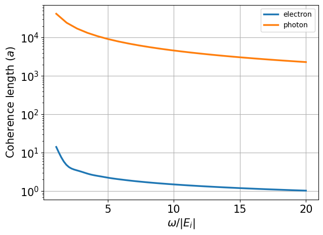
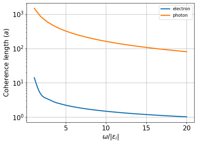
Figure 4: Comparison of transverse coherence length of the photoelectron (blue line) and characteristic size of the Bessel beam $\ell/\kappa$ for $\ell=3$ (orange line) depending on the photon energy $\omega$ for two different values of the Bessel beam opening angle: a) $\theta_{k}=1^{\circ}$; b) $\theta_{k}=30^{\circ}$. For larger energies of the photon the plots are qualitatively the same with the exception that the probability density is more localized in all directions.

Transverse coherence length of the photoelectron. Having derived the wave function of the outgoing electron in momentum representation, we now want to evaluate its Fourier transform and investigate the probability density in the coordinate space. First, we rewrite the delta-function in (1) as

$$\delta\left(\varepsilon_{i}+\omega-\frac{p^{2}}{2m}\right)=\frac{m}{p_{\perp}}\delta\left(p_{\perp}-\sqrt{2m(\varepsilon_{i}+\omega)-p_{z}^{2}}\right)$$ (27)

Then for the Bessel photon and zero impact parameter, the Fourier integral becomes

$\displaystyle\psi_{\text{ev}}(\bm{r})=e^{i\ell\varphi}\mathcal{N}m\sqrt{\frac{\kappa}{(2\pi)^{5}}}\int_{-\sqrt{2m(\varepsilon_{i}+\omega)}}^{\sqrt{2m(\varepsilon_{i}+\omega)}}J_{\ell}(p_{\perp}r_{\perp})$
$\displaystyle\times\Bigg{[}\frac{p_{\perp}}{\sqrt{2}}\big{[}d_{-1\Lambda}^{1}I_{\ell+1}(\alpha,\beta,0)-d_{1\Lambda}^{1}I_{\ell-1}(\alpha,\beta,0)\big{]}$
$\displaystyle+p_{z}d_{0\Lambda}^{1}I_{\ell}(\alpha,\beta,0)\Bigg{]}e^{ip_{z}z}dp_{z},$ (28)

where $p_{\perp}$, $\alpha$ and $\beta$ are the functions of the integration variable $p_{z}$. The remaining integral over $p_{z}$ in Eq. (28) can be computed numerically. For the incident LG photon the Fourier transform is done analogously with an additional numerical integration over $k_{\perp}$.

Fig. 2 demonstrates the probability density $|\psi_{\text{ev}}(\bm{r})|^{2}$ of the photoelectron if the incident light is Bessel beam with different values of OAM projection. Since we are not interested in the probability of the process, the absolute value of the probability density is unimportant. For this reason we normalize each distribution in a way that its maximal value equals $1$. For zero impact parameter the probability density is azimuthally symmetric, therefore we present only its dependence on radial coordinate $r_{\perp}$ and $z$. As seen from the figure, the photoelectron represents a wave packet localized around the position of the atom both in transverse and longitudinal directions. In case of Bessel beam with zero OAM the maximum of the probability density lies on the $z$ axis while for non-zero values of $\ell$ the wave packet has a well-known “doughnut shape” inherent to vortex states. It can also be seen that the radius of the first ring grows with the increase of $\ell$.

In Fig. 3 we display the probability density of the photoelectron for the incident LG beam with different values of the radial index $p$ and OAM $\ell$. Its waist $w_{0}$ is chosen as $0.5$ $\mu$m, which approximately equals the characteristic radius of the Bessel beam $1/\kappa$ for parameters listed under the Fig. 2. The first graph, Fig. 3 (a), corresponds to a Gaussian mode ($l=p=0$) and does not qualitatively differ from the case of Bessel beam with $\ell=0$. The Figs. 2 (b) and 3 (c) are also almost identical despite the key difference between the Bessel beam and the LG one: the latter is localized in the transverse plane whereas the former is not. It illustrates the fact that the width of the photoelectron wave packet does not depend on the transverse coherence of the incident light. This feature can be easily explained by the Eq. (28) as the transverse coordinate $r_{\perp}$ is contained only in the argument of the Bessel function $J_{\ell}(p_{\perp}r_{\perp})$ along with the transverse momentum $p_{\perp}=\sqrt{2m(\varepsilon_{i}+\omega)-p_{z}^{2}}$, which does not explicitly depend on $k_{\perp}$. Thus, we come to an important conclusion that it is the photon energy $\omega$ and not its transverse momentum $\kappa$ that determines the width of the photoelectron wave packet.

Let us now explicitly define the width (the transverse coherence length) of the electron packet as the distance from the $z$ axis to the point where the probability density is maximal. Further, we demonstrate the dependence of the electron transverse coherence length on the energy of the incident photon and compare it with the characteristic radius of the Bessel beam $\ell/\kappa$. As seen from the Fig. 4, the width of the electron packet, which is many orders of magnitude smaller than the Bessel beam radius, decreases with the increase of the photon energy. For $\omega\sim 20|\varepsilon_{i}|$ the localization becomes comparable to the Bohr radius $a$, which is the initial localization distance in the atom. The unbounded growth of the width as $\omega\to|\varepsilon_{i}|$ has little physical sense since the Born approximation that we use becomes invalid in case of extremely small energies of the outgoing electron.

Mesoscopic target. Up to this point, we have discussed the photoionization of a single atom positioned at a specific impact parameter relative to the propagation axis of the vortex beam. While recent advancements have made it possible to localize the target in this way [28, 29], the majority of photoionization experiments involve extended (mesoscopic) targets.

It is generally accepted in the related works that there is no coherence between photoelectrons emitted from different atoms [32]. Thus, photoemission from the localized target is described by averaging the cross section over a target distribution function [3, 4, 2]. However, the coherent effects in photoionization are also well-known: there are many theoretical and experimental works studying photoemission from diatomic molecule, which is regarded as analogue of Young’s double-slit experiment where the coherent emission of the electrons originating from two spatially separated sources gives rise to the interference patterns in the differential cross-section [33, 34, 35, 36, 2].

A peculiar feature of the evolved state arises in the hypothetical scenario when the photoionization occurs coherently from all atoms in the target which have the same phase of the wave function. It means that it is the amplitude of the process that should be averaged over the target rather than its squared absolute value (cross-section):

$$\widetilde{M}_{fi}^{\text{TW}}=\int\differential^{2}b\>n(\bm{b})M_{fi}^{\text{TW}}=\int b\>\differential b\>\differential\varphi_{b}n(\bm{b})M_{fi}^{\text{TW}}.$$ (29)

Let us, in addition, assume the mesoscopic target to be axially symmetric. One can notice that in this case the integration over $\varphi_{b}$ eliminates any term containing the factor $e^{in\varphi_{b}}$ in the amplitude (11). Thus, after the averaging over such a target the evolved state becomes a single-mode twisted state, just as in the scenario with $\bm{b}=0$. From an experimental viewpoint such a scenario could corresponds, for example, to the target represented by a cold atomic gas, where the coherence effects can play an important role [37, 38].

Incoherent photoionization: density matrix approach. Let us consider the density matrix of the (pure) evolved state

$$\hat{\rho}_{\text{ev}}=\ket{\text{ev}}\bra{\text{ev}}.$$ (30)

Unlike the regular density matrices, $\Tr(\hat{\rho})\neq 1,$ as $\Tr(\hat{\rho}_{\text{ev}})=\bra{\text{ev}}\ket{\text{ev}}=\int\frac{\differential^{3}p}{(2\pi)^{3}}|\psi_{\text{ev}}(\bm{p})|^{2}$, which diverges. Thus, if we would like to evaluate the mean values of observables using this density matrix, we should take the normalized definition: $\expectationvalue{\hat{A}}=\frac{\Tr\left(\hat{A}\hat{\rho}_{\text{ev}}\right)}{\Tr\left(\hat{\rho}_{\text{ev}}\right)}$. We can check that thus defined average value of the OAM projection upon the $z$ axis calculated with this density matrix equals $\ell$, $\expectationvalue{\hat{L}_{z}}=\ell$, when the impact parameter equals zero, see Appendix B.

Analogously, for a non-vanishing impact parameter we have

$\displaystyle\expectationvalue{\hat{L}_{z}}=$ $\displaystyle\frac{1}{\Tr(\hat{\rho}_{\text{ev}})}\sum_{\tilde{\ell}}\tilde{\ell}\int\frac{q_{\perp}\differential q_{\perp}\differential q_{z}\differential\varphi_{q}\differential\varphi_{q}^{\prime}}{(2\pi)^{6}}(2\pi)^{2}e^{i\tilde{\ell}(\varphi_{q}-\varphi_{q}^{\prime})}\psi_{\text{ev}}^{*}(q_{\perp},q_{z},\varphi_{q},\bm{b})\psi_{\text{ev}}(q_{\perp},q_{z},\varphi_{q}^{\prime},\bm{b})$
$\displaystyle=2\pi\mathcal{N}^{2}p^{2}\kappa\sum_{\tilde{\ell}}\tilde{\ell}\int\frac{q_{\perp}\differential q_{\perp}\differential q_{z}\differential\varphi_{q}\differential\varphi_{q}^{\prime}}{(2\pi)^{6}}(2\pi)^{2}e^{i(\tilde{\ell}-\ell)\varphi_{q}}e^{-i(\tilde{\ell}-\ell)\varphi_{q}^{\prime}}\delta\left(\varepsilon_{i}+\omega-\frac{q^{2}}{2m}\right)$
$\displaystyle\times\delta\left(\varepsilon_{i}+\omega-\frac{q^{\prime 2}}{2m}\right)\Bigg{[}\frac{q_{\perp}}{\sqrt{2}}\left[d_{-1\Lambda}^{1}I_{\ell+1}(\alpha,\beta,\bm{b},\varphi_{q})-d_{1\Lambda}^{1}I_{\ell-1}(\alpha,\beta,\bm{b},\varphi_{q})\right]+q_{z}d_{0\Lambda}^{1}I_{\ell}(\alpha,\beta,\bm{b},\varphi_{q})\Bigg{]}^{*}$
$\displaystyle\times\Bigg{[}\frac{q_{\perp}^{\prime}}{\sqrt{2}}\left[d_{-1\Lambda}^{1}I_{\ell+1}(\alpha^{\prime},\beta^{\prime},\bm{b},\varphi_{q}^{\prime})-d_{1\Lambda}^{1}I_{\ell-1}(\alpha^{\prime},\beta^{\prime},\bm{b},\varphi_{q}^{\prime})\right]+q_{z}^{\prime}d_{0\Lambda}^{1}I_{\ell}(\alpha^{\prime},\beta^{\prime},\bm{b},\varphi_{q}^{\prime})\Bigg{]}\bigg{/}{\Tr(\hat{\rho}_{\text{ev}})}.$ (31)

Let us again suppose that the target is small enough and expand expression (31) in powers of $\kappa b$ up to the linear terms. Recall that

$\displaystyle I_{\ell}(\alpha,\beta,\bm{b},\varphi_{p})\approx I_{n}(\alpha,\beta,0)-\frac{i\kappa b}{2}e^{-i\varphi_{b}}e^{i\varphi_{p}}I_{\ell+1}(\alpha,\beta,0)$
$\displaystyle-\frac{i\kappa b}{2}e^{i\varphi_{b}}e^{-i\varphi_{p}}I_{\ell-1}(\alpha,\beta,0).$ (32)

Thus, any term in (31) that is proportional to $\kappa b$ has the form of $\sim I_{n}(\alpha,\beta,0)I_{m}(\alpha^{\prime},\beta^{\prime},0)e^{\pm i(\varphi_{b}-\varphi_{q})}$ or $\sim I_{n}(\alpha,\beta,0)I_{m}(\alpha^{\prime},\beta^{\prime},0)e^{\pm i(\varphi_{b}-\varphi_{q}^{\prime})}$. After the integration over $\varphi_{q}$ (or $\varphi_{q}^{\prime}$) in Eq. (31) the Kronecker delta $\delta_{\tilde{\ell},\ell\pm 1}$ appears. Then this term is eliminated by the second azimuthal integral, as

$$\int_{0}^{2\pi}e^{i(\tilde{\ell}-\ell)\varphi_{q}}=0$$ (33)

when $\tilde{\ell}=\ell\pm 1$. Thus, we come to the conclusion that in the first order expansion in the parameter $\kappa b$

$$\expectationvalue{\hat{L}_{z}}=\ell$$ (34)

despite the small, but non-vanishing impact parameter.

Importantly, the incoherent averaging over the target, which is generally understood as the averaging of the differential cross-section, can be interpreted in terms of the density matrix. In this case the outgoing electron simply represents a mixed state of electron states scattered from different atoms rather than a coherent superposition. We now introduce the averaged density matrix

$$\hat{\rho}_{\text{ev}}^{\prime}=\int\differential^{2}b\>n(\bm{b})\hat{\rho}_{\text{ev}}(\bm{b}).$$ (35)

If the target is small enough in the sense that $\kappa b\ll 1$, the mean value of the OAM projection of each state in the mixture approximately equals $\ell$, and thus for the whole state we find that

$$\expectationvalue{\hat{L}_{z}}^{\prime}=\frac{1}{\Tr(\hat{\rho}_{\text{ev}}^{\prime})}\Tr\left(\hat{L}_{z}\hat{\rho}_{\text{ev}}^{\prime}\right)=\ell.$$ (36)

Although the described photoelectron state is not pure, it may be deemed twisted in the sense of having a definite expectation value of the OAM projection.

Conclusion. In summary, we have studied theoretically the final evolved state of the electron that is emitted in the ionization of hydrogen–like atom by a vortex light beam. The non-relativistic first-order perturbation theory was applied to derive the state of the photoelectron as it evolves from the process itself, without specifying any detection scheme. We have shown that the emitted photoelectron generally represents a localized wave packet with a well-defined projection of the orbital angular momentum (OAM) onto the quantization axis of the photon TAM.

The transverse size (coherence length) of the electron packet is shown to be solely governed by the energies of the initial bound electron and incident photon. The ionization of an extended atomic target instead of a single atom does not significantly violate the OAM of the resulting electron as long as the size of the target does not exceed the transverse size of the light beam. Although we have considered only nonrelativistic electron and have neglected spin effects, it can be expected that in a rigorous relativistic framework the angular momentum is also fully transferred from the photon to the electron. However, in this case, the outgoing particle has a certain value of TAM projection rather than OAM, and the splitting of the TAM into spin and orbital parts is ambiguous for both particles [39].

Therefore, we propose that ionization by vortex light beams can be used to generate vortex electrons in experimental setups where the usage of other generation techniques (diffraction grating, phase plate, magnetic monopole, etc. [11]) is hampered for some reason. For instance, such an approach could be used to produce high-energy twisted electrons via irradiating photocathodes at various accelerator facilities, such as LINAC-200 at JINR, Dubna. This could open up opportunities for the experimental study of vortex state collisions and various radiation processes [12, 20, 21, 10, 40, 41, 42, 13, 14].

More results related to the ITMO-JINR project on relativistic vortex electron generation could be expected in near future. In particular, we plan to take into account the possibility of OAM redistribution between the photoelectron and the atomic center of mass (similarly to [29, 43, 44]), and the processes of relaxation due to interaction with the adjacent atoms.

Acknowledgments. We are thankful to V. Ivanov for his initial contribution to this project. We are also grateful to G. Sizykh and D. Grosman for many valuable discussions and advice. The studies on ionization with the Bessel beam are supported by the Ministry of Science and Higher Education of the Russian Federation (agreement No. 075-15-2021-1349). The research on photoionization with LG beams is supported by the Russian Science Foundation (Project No. 23-62-10026; [9]). The developments on incoherent photoionization by A.C. and D.K. are supported by the Government of the Russian Federation through the ITMO Fellowship and Professorship Program. Analysis of the transverse coherence length of the photoelectron by D.K. is also supported by the Foundation for the Advancement of Theoretical Physics and Mathematics “BASIS”.

Appendix A Polarization vector decomposition

Let us take a plane wave photon in representation (6) and write down its polarization vector in terms of spherical angles $\theta_{k}$ and $\varphi_{k}$ [7]

$$\bm{e}_{\bm{k}\Lambda}=\sum\limits_{\sigma=0,\pm 1}e^{-i\sigma\varphi_{k}}d_{\sigma\Lambda}^{1}(\theta_{k})\bm{\chi}_{\sigma},$$ (37)

where $d^{J}_{MM^{\prime}}(\theta)$ are the small Wigner functions [45] and the basis vectors are defined as follows:

$\displaystyle\bm{\chi}_{0}=\begin{pmatrix}0\\ 0\\ 1\end{pmatrix},\,\bm{\chi}_{\pm 1}=\mp\frac{1}{\sqrt{2}}\begin{pmatrix}1\\ \pm i\\ 0\end{pmatrix};$ (38)
$\displaystyle\bm{\chi}_{1}\bm{\chi}_{-1}=\bm{\chi}_{-1}\bm{\chi}_{1}=-1,\ \bm{\chi}_{\pm 1}\bm{\chi}_{\pm 1}=0.$ (39)

Then, we can express the vector $\bm{n}=\bm{p}/p$ in the same basis as polarization vector $\bm{e}_{\bm{k}\Lambda}$:

$\displaystyle\bm{n}=\bm{\chi}_{0}\cos{\theta_{p}}-\frac{1}{\sqrt{2}}(\bm{\chi}_{1}e^{-i\varphi_{p}}-\bm{\chi}_{-1}e^{i\varphi_{p}})\sin{\theta_{p}},$ (40)

and the scalar product in Eq. (10) can be decomposed as follows:

$$\bm{e}_{\bm{k}\Lambda}\bm{n}=\sum\limits_{\sigma=0,\pm 1}e^{-i\sigma\varphi_{k}}d_{\sigma\Lambda}^{1}(\theta_{k})\bm{\chi}_{\sigma}\bm{n}\\ =\frac{\sin\theta_{p}}{\sqrt{2}}e^{i(\varphi_{k}-\varphi_{p})}d_{-1\Lambda}^{1}(\theta_{k})+d_{0\Lambda}^{1}(\theta_{k})\cos\theta_{p}\\ -\frac{\sin\theta_{p}}{\sqrt{2}}e^{-i(\varphi_{k}-\varphi_{p})}d_{1\Lambda}^{1}(\theta_{k}).$$ (41)

Appendix B Calculating $\expectationvalue{\hat{L}_{z}}$ with density matrix

Here we check that the average value of the OAM projection upon the $z$ axis calculated with this density matrix equals $\ell$ when the impact parameter equals zero.

Let us start with the definition

$\displaystyle\expectationvalue{\hat{L}_{z}}$ $\displaystyle=$ $\displaystyle\frac{1}{\Tr(\hat{\rho}_{\text{ev}})}\Tr\left(\hat{L}_{z}\hat{\rho}_{\text{ev}}\right)$ (42)
$\displaystyle=$ $\displaystyle\frac{1}{\Tr(\hat{\rho}_{\text{ev}})}\int\frac{\differential^{3}q}{(2\pi)^{3}}\bra{\bm{q}}\hat{L}_{z}\hat{\rho}\ket{\bm{q}}$ (43)
$\displaystyle=$ $\displaystyle\frac{1}{\Tr(\hat{\rho}_{\text{ev}})}\int\frac{\differential^{3}q\differential^{3}q^{\prime}}{(2\pi)^{6}}\bra{\bm{q}}\hat{L}_{z}\ket{\bm{q}^{\prime}}\bra{\bm{q}^{\prime}}\hat{\rho}\ket{\bm{q}},$ (44)

where

$\displaystyle\bra{\bm{q}^{\prime}}\hat{\rho}\ket{\bm{q}}=$ $\displaystyle\psi_{\text{ev}}^{*}(\bm{q})\psi_{\text{ev}}(\bm{q}^{\prime}),$ (45)
$\displaystyle\bra{\bm{q}}\hat{L}_{z}\ket{\bm{q}^{\prime}}=$ $\displaystyle\sum_{\tilde{\ell}}\int\frac{\tilde{q}_{\perp}\differential\tilde{q}_{\perp}\differential\tilde{q}_{z}}{(2\pi)^{2}}\bra{\bm{q}}\hat{L}_{z}\ket*{\tilde{q}_{\perp}\tilde{q}_{z}\tilde{\ell}}\bra*{\tilde{q}_{\perp}\tilde{q}_{z}\tilde{\ell}}\ket{\bm{q}^{\prime}}.$ (46)

With the projection of a Bessel vortex state on a plane wave being

$$\bra*{\tilde{q}_{\perp}\tilde{q}_{z}\tilde{\ell}}\ket{\bm{q}}=e^{-i\tilde{\ell}\varphi_{q}}\frac{(2\pi)^{2}}{\sqrt{\tilde{q}_{\perp}}}\delta(\tilde{q}_{\perp}-q_{\perp})\delta(\tilde{q}_{z}-q_{z}),$$ (47)

we can calculate

$$\bra{\bm{q}}\hat{L}_{z}\ket{\bm{q}^{\prime}}=\sum_{\tilde{\ell}}\tilde{\ell}(2\pi)^{2}e^{i\tilde{\ell}(\varphi_{q}-\varphi_{q}^{\prime})}\delta(q_{\perp}-q_{\perp}^{\prime})\delta(q_{z}-q_{z}^{\prime})\frac{1}{q_{\perp}}.$$ (48)

Then, with $\differential^{3}q=q_{\perp}\differential q_{\perp}\differential q_{z}\differential\varphi_{q}$, we can show

$$\expectationvalue{\hat{L}_{z}}=\frac{1}{\Tr(\hat{\rho}_{\text{ev}})}\int\frac{\differential^{3}q\differential^{3}q^{\prime}}{(2\pi)^{6}}\sum_{\tilde{\ell}}\tilde{\ell}(2\pi)^{2}e^{i\tilde{\ell}(\varphi_{q}-\varphi_{q}^{\prime})}\delta(q_{\perp}-q_{\perp}^{\prime})\delta(q_{z}-q_{z}^{\prime})\frac{1}{q_{\perp}}\psi_{\text{ev}}^{*}(\bm{q})\psi_{\text{ev}}(\bm{q}^{\prime})\\ =\frac{1}{\Tr(\hat{\rho}_{\text{ev}})}\sum_{\tilde{\ell}}\tilde{\ell}\int\frac{q_{\perp}\differential q_{\perp}\differential q_{z}\differential\varphi_{q}\differential\varphi_{q}^{\prime}}{(2\pi)^{6}}(2\pi)^{2}e^{i\tilde{\ell}(\varphi_{q}-\varphi_{q}^{\prime})}\underbrace{\psi_{\text{ev}}^{*}(q_{\perp},q_{z},\varphi_{q})}_{\chi^{*}(q_{\perp},q_{z})e^{-i\ell\varphi_{q}}}\underbrace{\psi_{\text{ev}}(q_{\perp},q_{z},\varphi_{q}^{\prime})}_{\chi(q_{\perp},q_{z})e^{i\ell\varphi_{q}^{\prime}}}\\ =\frac{1}{\Tr(\hat{\rho}_{\text{ev}})}\sum_{\tilde{\ell}}\tilde{\ell}\delta_{\ell\tilde{\ell}}\int\frac{q_{\perp}\differential q_{\perp}\differential q_{z}\differential\varphi_{q}}{(2\pi)^{6}}(2\pi)^{3}e^{i(\tilde{\ell}-\ell)\varphi_{q}}|\chi(q_{\perp},q_{z})|^{2}\\ =\frac{1}{\Tr(\hat{\rho}_{\text{ev}})}\ell\int\frac{q_{\perp}\differential q_{\perp}\differential q_{z}\differential\varphi_{q}}{(2\pi)^{3}}|\psi_{\text{ev}}(\bm{q})|^{2}=\ell$$ (49)

References