AdjointDEIS: Efficient Gradients for Diffusion Models
Abstract
The optimization of the latents and parameters of diffusion models with respect to some differentiable metric defined on the output of the model is a challenging and complex problem. The sampling for diffusion models is done by solving either the probability flow ODE or diffusion SDE wherein a neural network approximates the score function or related quantity, allowing a numerical ODE/SDE solver to be used. However, naïve backpropagation techniques are memory intensive, requiring the storage of all intermediate states, and face additional complexity in handling the injected noise from the diffusion term of the diffusion SDE. We propose a novel method based on the stochastic adjoint sensitivity method to calculate the gradients with respect to the initial noise, conditional information, and model parameters by solving an additional SDE whose solution is the gradient of the diffusion SDE. We exploit the unique construction of diffusion SDEs to further simplify the formulation of the adjoint diffusion SDE and use a change-of-variables to simplify the solution to an exponentially weighted integral. Using this formulation we derive a custom solver for the adjoint SDE as well as the simpler adjoint ODE. The proposed adjoint diffusion solvers can efficiently compute the gradients for both the probability flow ODE and diffusion SDE for latents and parameters of the model. Lastly, we demonstrate the effectiveness of the adjoint diffusion solvers on the face morphing problem.
1 Introduction
Diffusion models are a large family of state-of-the-art generative models which learn to map samples drawn from white Gaussian noise into the data distribution [1, 2]. These diffusion models have achieved state-of-the-art performance on prominent tasks such as image generation [3, 4, 5], audio generation [6], or video generation [7]. Often the state-of-the-art models are quite large and training them is prohibitively expensive [8]. As such it is fairly common to adapt a pre-trained model to a specific task for post-training. This way the generative model can learn new concepts, identities, or tasks without needing to training the whole model [9, 10, 11]. Additional work has also proposed algorithms for guiding the generative process of the diffusion models [12, 13].
One method to guide or direct the generative process is to solve an optimization problem w.r.t. some loss function defined on the image space . This loss functions works on the output of the diffusion model and assess how “good” the output is. However, the diffusion model works by iteratively removing noise until a clean sample is reached. As such we need to be able to efficiently backpropagate gradients through the entire generative process. As Song et al. [14] showed the diffusion SDE can be simplified to an associated ODE, and as such many efficient ODE/SDE solvers have been developed for diffusion models [15, 16, 17]. However, naïvely applying backpropagation to the diffusion model is inflexible and memory intensive; moreover, such an approach is not trivial to apply to the diffusion models that used an SDE solver instead of an ODE solver.
Inspired by the work of Chen et al. [18] and their application of the method of adjoint sensitivity to model ODEs with neural networks, we propose AdjointDEIS a novel technique for calculating the gradient of the noisy states, and other parameters, of the diffusion model using the method of adjoint sensitivity. We exploit the unique construction of diffusion models to greatly simplify the adjoint ODE into a problem with exponential integrators which reduces the discretization errors of the adjoint ODE. We then design a custom second-order multi-step method for solving the adjoint ODE. Additionally, we extend this technique to work for diffusion SDEs and not just ODEs. Lastly, we evaluate the proposed techniques on the face morphing problem to illustrate the use of this technique for guided generation problems. The contribution of this work can be summarized as follows:
-
1.
We propose a method for calculating gradients of diffusion models.
-
2.
To the best of our knowledge, AdjointDEIS is the first general backpropagation technique for diffusion models that use an SDE solver for sampling and can supply gradients for network weights, conditional information, and intermediate noisy states.
-
3.
We develop custom first and second order solvers for the adjoint ODE/SDE.
-
4.
We illustrate the effectiveness of AdjointDEIS for guided generation on the face morphing problem.
2 Diffusion Models
In this section we provide a brief overview of diffusion models. Diffusion models learn a generative process by first perturbing the data distribution into an isotropic Gaussian by progressively adding Gaussian noise to the data distribution, then a neural network is trained to preform denoising steps, allowing for sampling of the data distribution via sampling of a Gaussian distribution [2, 8]. Assume we have an -dimensional random variable with some distribution . Then diffusion models begin by diffusing according to the diffusion SDE [2], an Itô SDE given as
| (2.1) |
where denotes time with fixed constant , and denote the drift and diffusion coefficients, and denotes the standard Wiener process. The trajectories of follow the distributions with and . Under some regularity conditions Song et al. [14] showed that Equation 2.1 has a reverse process as time runs backwards from to with initial marginal distribution governed by
| (2.2) |
where is the standard Wiener process as time runs backwards. Solving Equation 2.2 is what allows diffusion models to draw samples from by sampling . The unknown term in Equation 2.2 is the score function , which in practice is modeled by a neural network that estimates the scaled score function, , or some closely related quantity like -prediction [19, 1, 2].
2.1 Probability Flow ODE
The practical choice of a step size when discretizing SDEs is limited by the randomness of the Wiener process as a large step size, i.e., a small number of steps, can cause non-convergence, particularly in high-dimensional spaces [15]. Sampling an equivalent Ordinary Differential Equation (ODE) over an SDE would enable for faster sampling. Song et al. [14] showed there exists an Ordinary Differential Equation (ODE) whose marginal distribution at time are identical to that of Equation 2.2 given as
| (2.3) |
The ODE in Equation 2.3 is known as the probability flow ODE (PF ODE) [14]. As the noise prediction network, , is trained to model the scaled score function, Equation 2.3 can be parameterized as
| (2.4) |
w.r.t. the noise prediction network. We refer to this ODE as the empirical PF ODE following the nomenclature of Song et al. [20].
While there exist several popular choices for the drift and diffusion coefficients, we opt to use the de facto choice which is known as the Variance Preserving (VP) type diffusion SDE [21, 1, 14]. The coefficients for VP-type SDEs are given as
| (2.5) |
which corresponds to sampling from the distribution .
3 Adjoint Diffusion ODEs
We begin with the much simpler case of diffusion ODEs. A key insight of this work is the connection between the adjoint ODE used in Neural ODEs by Chen et al. [18] and specialized ODE/SDE solvers by Lu et al. [15, 16], Zhang and Chen [17] for diffusion models. We propose a method for optimizing the latents and of a diffusion model, with noise prediction network , w.r.t. a loss function, defined on the output where is the initial noise and is the, optional, conditional information supplied to the noise prediction network. In order to optimize the latents, the gradients of and w.r.t. the loss function needs to be calculated. However, as the output of the diffusion model is calculated by solving the PF ODE, calculating the gradients requires a continuous backpropagation through time. To find these gradients, we propose to solve a dual ODE which we call the adjoint probability flow ODE.
3.1 Empirical Adjoint Probability Flow ODE
The Probability Flow ODE with a neural network based approximator of the score function is noted by Song et al. [14] to be a type of Neural ODE [18]. Similar to the adjoint ODE used for backpropagation through Neural ODEs, we use the adjoint sensitivity method from Pontryagin et al. [22] to compute the gradients and . Let describe the R.H.S of Equation 2.4, defined as
| (3.1) |
Let denote the adjoint state, the dynamics of which evolve with another ODE
| (3.2) |
as time flows forwards from to , i.e., the reverse flow of time w.r.t. the PF ODE. The gradients of the loss w.r.t. and are expressed as the solution to another set of ODEs
| (3.3) | ||||
| (3.4) |
These constructions follow from Chen et al. [18, Appendix B.2] and are a straightforward application of the method of adjoint sensitivity to . Together this system of ODEs form the empirical adjoint PF ODE which allows for calculation of the gradients of the initial noise and conditional information of diffusion models.
3.2 Simplified Formulation of the Empirical Adjoint Probability Flow ODE
We show that rather than treating as a black box, the specific structure of the PF ODE is carried over to the adjoint PF ODE, allowing the adjoint PF ODE to be simplified into a special exact formulation.
Taking into consideration the structure of the empirical PF ODE, Equation 3.2 becomes
| (3.5) |
by expanding out the gradient of w.r.t. . Due to the gradient of the drift term in Equation 3.5, further manipulations are required to put the empirical adjoint PF ODE into a sufficiently “nice” form. We follow the approach used by Lu et al. [15] and Zhang and Chen [17] to simplify the empirical PF ODE with the use of exponential integrators and a change of variables. By applying the integrating factor to Equation 3.5, the following ODE is expressed as
| (3.6) |
We introduce , a new variable which greatly simplifies the ODE. With this change of variables, Equation 3.6 becomes
| (3.7) |
where and therefore . To further simplify Equation 3.7, let be one half of the log-SNR. Then the empirical adjoint PF ODE can be expressed in terms of an exponential integrator leading to:
Proposition 3.1.
Given an initial values at time , the solution at time of the adjoint empirical PF ODE in Equation 3.7 is
| (3.8) |
and as is a strictly decreasing function w.r.t. and therefore it has an inverse function which satisfies , and, with abuse of notation, we let , , &c. Importantly, just like with the usage of exponential integrators for solving the empirical PF ODE [15, 17], the linear term is computed exactly, thereby removing the linear term error entirely.
The numerical solver for the adjoint empirical PF ODE, now in light of Equation 3.8, only needs to focus on approximating the exponentially weighted integral of from to , a well-studied problem in the literature on exponential integrators [23, 24]. To approximate this integral, we evaluate the Taylor expansion of the vector Jacobian product to further simplify the ODE. For , the -th Taylor expansion at is
| (3.9) |
Plugging this expansion into Equation 3.8 and letting yields
| (3.10) |
With this expansion the number of estimated terms is further reduced as the exponentially weighted integral can be solved analytically by applying times integration-by-parts [15, 25]. Therefore, the only errors in solving this ODE occur in the approximation of the -th order derivatives of the vector Jacobian product and the high-order error terms . In the first-order scenario of and dropping the high-order error term , the following approximation for Equation 3.8 becomes
| (3.11) |
However, this is still in terms of and not the true quantity of interest , this is simply remedied by changing variables back to . For the adjoint conditional and parameter ODEs, let denote the integral from to of the R.H.S. of Equation 3.3 plus an initial value , and likewise for . The complete system of ODE solvers for calculating the gradients is found below
AdjointDEIS-1 Given an initial adjoint state at time , the solution at time is approximated by
| (3.12) |
likewise the gradients w.r.t. and w.r.t. are approximated as
| (3.13) | ||||
| (3.14) |
3.3 Multi-step Solvers for Adjoint Diffusion ODE
High-order expansions of Equation 3.10 require estimations of the -th order derivatives of the vector Jacobian product which can be approximated via multi-step methods, such as Adams-Bashforth methods [26]. This has the added benefit of reduced computational overhead, as the multi-step method just reuses previous values to approximate the high-order derivatives. Moreover, multi-steps are empirically more efficient than single-step methods [26]. Combining the Taylor expansions in Equation 3.9 with techniques for designing multi-step solvers, we propose a novel multi-step second-order solver for the adjoint empirical PF ODE which we call AdjointDEIS-2M. This algorithm combines the previous values of the vector Jacobian product at time and time to predict without any additional intermediate values.
AdjointDEIS-2M We assume having a previous solution and model output at time , let denote . Then the solution at time to Equation 3.5 is estimated to be
| (3.15) |
likewise the gradients w.r.t. and w.r.t. are approximated as
| (3.16) | ||||
| (3.17) |
The full derivation is provided in Section A.2.
4 Adjoint Diffusion SDEs
As recent work [27, 28] has shown, diffusion SDEs have useful properties over PF ODEs for image manipulation and editing. In particular, it has been shown that PF ODEs are invariant in Nie et al. [28, Theorem 3.2] and that diffusion SDEs are contractive in Nie et al. [28, Theorem 3.1], i.e., any gap in the mismatched prior distributions and for the true distribution and edited distribution will remain between and , whereas for diffusion SDEs the gap can be reduced betwen and as tends towards . Motivated by this reasoning, we present a framework for solving the adjoint diffusion SDE using exponential integrators.
The empirical diffusion SDE [14] in the Itô sense is given as
| (4.1) |
Samples can be drawn from diffusion models by solving Equation 4.1 with a numerical SDE solver. In order to calculate the gradients of the diffusion model w.r.t. empirical diffusion SDE, it is necessary that the SDE be solved as time runs forwards from to . Unfortunately, Itô SDEs are not easily reversible in time through a simple sign change like with ODEs, which would be quite useful as the diffusion SDE needs to be calculated both forwards and backwards. However, the Stratonovich stochastic integral provides a handy tool for going both forwards and backwards in time. Following in the vein of [29, 30], we follow the treatment of Kunita [31] for the forward and backward Stratonovich integrals using two-sided filtration. Let be a two-sided filtration, where is the -algebra generated by for such that . For a continuous semi-martingale adapted to the forward filtration , the Stratonovich stochastic integral is given as
| (4.2) |
where is a partition of the interval and . Consider the backwards Wiener process that is adapted to the backward filtration , then for a continuous semi-martingale adapted to the backward filtration, the backward Stratonovich integral is
| (4.3) |
Itô SDEs can be easily converted into the Stratonovich form111For some Itô SDE of the form with differentiable function , there exists a corresponding Stratonovich SDE of the form and fortunately the diffusion term in Equation 4.1 is simply , which is a deterministic function. Then the Itô integral and Stratonovich integral, are essentially222The interpretation of the two integrals are different and require slightly different treatment, but for the purposes of this paper and are essentially the same. Further details can be found in [31]. the same with no correction term in the drift coefficient. Thus, for some initial state the empirical diffusion SDE in Equation 4.1 is equivalent to
| (4.4) |
Throughout this paper we assume that is Lipschitz w.r.t. its first parameter, , as is commonly assumed in other works [15, 20] and we also assume that have bounded first derivatives and therefore the SDE has a unique strong solution. Given a realization of the backwards Wiener process, there exists a smooth mapping called the stochastic flow such that is the solution at time of the process starting at at time . This defines a collection of continuous maps from to itself. These maps are diffeomorphisms and satisfy the flow property such that
| (4.5) |
and have a backwards flow that satisfies the backwards SDE
| (4.6) |
see Li et al. [29, Theorem 2.1]. Notably the coefficients in Equation 4.4 and Equation 4.6 differ only by a negative sign.
Following prior work on designing ODE/SDE solvers for diffusion models [15, 17, 16, 25] we use the variation-of-parameters formula to rewrite Equation 4.4 as
| (4.7) |
transforming it into an SDE with exponential integrators [23]. While the linear and non-linear terms have been studied extensively [15, 16, 17], the stochastic term has only been studied in the Itô sense [25]. However, as the diffusion term is simply the deterministic function , this can be straightforwardly converted to the more familiar stochastic integral in the Itô sense. As shown in Lu et al. [16] this SDE has a first-order solver of the form
| (4.8) |
where and in this context.
4.1 Solving the Backwards Empirical Diffusion SDE
To solve the SDE backwards in time we follow the approach initially proposed by Wu and la Torre [32] and used by later works [28]. Given a particular realization of the Wiener process that admits , then for two samples and the noise can be calculated by rearranging Equation 4.8 to find
| (4.9) |
With this the sequence of added noises can be calculated which will exactly reconstruct the original input from the initial realization of the Wiener process. This technique is referred to as Cycle-SDE after the CycleDiffusion paper [32].
4.2 Derivation of Adjoint Empirical Diffusion SDE
Let denote the adjoint flow of the gradients of w.r.t. from some terminal time to an initial time . By the chain rule this is equivalent to . Let the backwards adjoint flow be denoted by , and note that . Li et al. [29] show that the adjoint backwards flow satisfies the adjoint SDE
| (4.10) |
Notably the diffusion term in Equation 4.10 becomes zero as . Therefore, the adjoint flow, , evolves with an ODE and not an SDE. Thus, while the backwards flow evolves with an SDE, the adjoint flow can be solved with a much simpler ODE solver. Therefore, the same AdjointDEIS solvers used earlier in Section 3 can be used here with a correction term of 2 to account for the difference in weighting term for the neural network for empirical PF ODEs vs for empirical diffusion SDEs. Thus we present the following
SDE-AdjointDEIS-1 Given an initial adjoint state at time the solution at time is approximated by
| (4.11) |
likewise the gradients w.r.t. and w.r.t. are approximated as
| (4.12) | ||||
| (4.13) |
5 Experiments
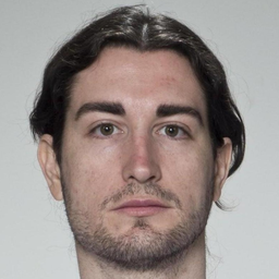
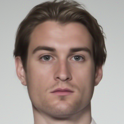
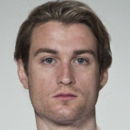
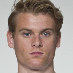
To illustrate the efficacy of the AdjointDEIS technique, we examine the application of guided generation for the face morphing attack. The face morphing attack is a new emerging attack on biometric systems. This attack works by creating a singular morphed face image that shares biometric information with the two contributing faces and [33, 34, 35]. A successfully created morphed face image can trigger a false accept with either of the two contributing identities in the targeted Face Recognition (FR) system, see Figure 1 for an illustration. Recent work in this space has explored the use of diffusion models to generate these powerful attacks [33, 36, 37]. All prior work on diffusion-based face morphing used a pre-trained diffusion autoencoder [38] trained on the FFHQ [39] dataset at resolution. We illustrate the use of AdjointDEIS by modifying the Diffusion Morph (DiM) architecture proposed by Blasingame and Liu [33] to use the AdjointDEIS solvers to find the optimal initial noise and conditional . The AdjointDEIS is used to calculate the gradients with respect to the identity loss [37] defined as
| (5.1) | ||||
| (5.2) | ||||
| (5.3) |
where , and is an FR system which embeds images into a vector space which is equipped with a measure of distance, . We used the ArcFace FR system for the identity loss.
We run our experiments on the SYN-MAD 2022 [40] morphed pairs which are constructed from the Face Research Lab London dataset [41], more details in Section E.3. The morphed images are evaluated against three FR systems, the ArcFace [42], ElasticFace [43], and AdaFace [44] models, further details are found in Section E.4. To measure the efficacy of a morphing attack, the Mated Morph Presentation Match Rate (MMPMR) metric [45] is used. The MMPMR metric as proposed by Scherhag et al. [45] is defined as
| (5.4) |
where is the verification threshold, is the similarity score of the -th subject of morph , is the total number of contributing subjects to morph , and is the total number of morphed images.
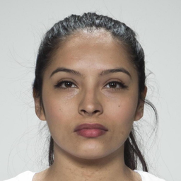
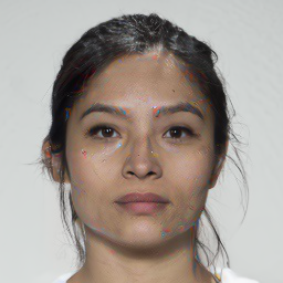
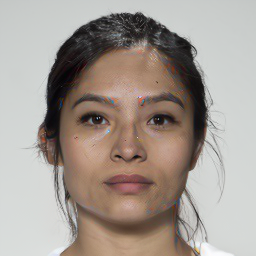

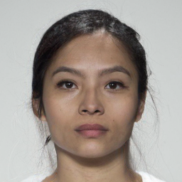

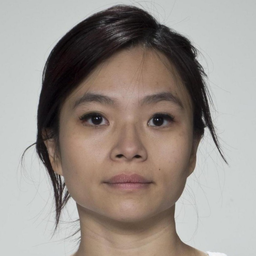
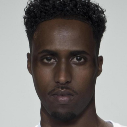
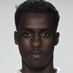

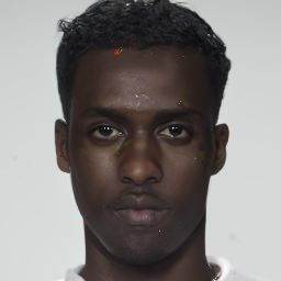
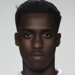
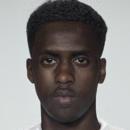
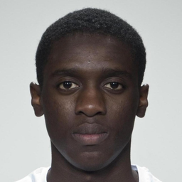
In Figure 2 we provide a visual comparison between other diffusion models for face morphing and our modification of adding adjoint optimization. We observe that the AdjointDEIS generated morphs have less visual artefacts, see the red highly saturated splotches on some of the other morphs, have more natural lighting, and have a more realistic skin texture. In Figure 1 it is quite obvious that the morphed image generated using the SDE-AdjointDEIS solver has a far more realistic skin texture than the AdjointDEIS solver. This is unsurprising as the prior work has shown how the PF ODE is invariant [28] and since morphing, at its most fundamental, is an averaging of two faces.
| MMPMR() | ||||
|---|---|---|---|---|
| Morphing Attack | NFE() | AdaFace | ArcFace | ElasticFace |
| DiM-A [33] | 350 | 92.23 | 90.18 | 93.05 |
| Fast-DiM [36] | 300 | 92.02 | 90.18 | 93.05 |
| Morph-PIPE [37] | 2350 | 95.91 | 92.84 | 95.5 |
| DiM + AdjointDEIS | 1250 | 96.32 | 93.25 | 96.32 |
| DiM + SDE-AdjointDEIS | 750 | 95.71 | 94.68 | 96.32 |
In Table 1 we present the effectiveness of the morphing attacks against the three FR systems. We observe that both morphing attacks that use the AdjointDEIS solver for adjoint optimization outperform all existing face morphing attacks. Interestingly, the AdjointDEIS attack slightly outperforms the SDE-AdjointDEIS on the AdaFace and ElasticFace FR systems. Overall, this experiment shows the usefulness of the AdjointDEIS technique for guided generation tasks.
6 Conclusion
We present a unified view on calculating the gradients of diffusion models in both the ODE and SDE formulations using the method of adjoint sensitivity. To this end we propose AdjointDEIS a suite of solvers for efficient solving the adjoint empirical PF ODEs and diffusion SDEs. Like its namesake, the AdjointDEIS solver exploits the semi-linearity of the PF ODE to greatly simplify exact solution to the adjoint ODE. Then inspired by numerical methods for exponential integrators we propose both first-order and second-order solvers for the diffusion ODE. We then extend this approach to develop custom solvers for the adjoint SDE and discover that the adjoint diffusion SDE simplifies to another ODE. Our experimental results show that the gradients produced by AdjointDEIS can be used for guided generation tasks.
Limitations Despite the great initial performance of the AdjointDEIS solver further experimental analysis on different kinds of guided generation tasks still needs to be done. Moreover, while shown the application of adjusting the network weights with AdjointDEIS was not shown in this work. Theoretically, we do not prove convergence rates for our proposed solver, although this can potentially be addressed based on existing work [15].
References
- Ho et al. [2020] Jonathan Ho, Ajay Jain, and Pieter Abbeel. Denoising diffusion probabilistic models. In H. Larochelle, M. Ranzato, R. Hadsell, M.F. Balcan, and H. Lin, editors, Advances in Neural Information Processing Systems, volume 33, pages 6840–6851. Curran Associates, Inc., 2020. URL https://proceedings.neurips.cc/paper/2020/file/4c5bcfec8584af0d967f1ab10179ca4b-Paper.pdf.
- Song et al. [2021a] Jiaming Song, Chenlin Meng, and Stefano Ermon. Denoising diffusion implicit models. In International Conference on Learning Representations, 2021a. URL https://openreview.net/forum?id=St1giarCHLP.
- Rombach et al. [2022] Robin Rombach, Andreas Blattmann, Dominik Lorenz, Patrick Esser, and Björn Ommer. High-resolution image synthesis with latent diffusion models. In Proceedings of the IEEE/CVF Conference on Computer Vision and Pattern Recognition (CVPR), pages 10684–10695, June 2022.
- Ramesh et al. [2022] Aditya Ramesh, Prafulla Dhariwal, Alex Nichol, Casey Chu, and Mark Chen. Hierarchical Text-Conditional Image Generation with CLIP Latents. arXiv e-prints, art. arXiv:2204.06125, April 2022. doi: 10.48550/arXiv.2204.06125.
- Saharia et al. [2022] Chitwan Saharia, William Chan, Saurabh Saxena, Lala Li, Jay Whang, Emily L Denton, Kamyar Ghasemipour, Raphael Gontijo Lopes, Burcu Karagol Ayan, Tim Salimans, Jonathan Ho, David J Fleet, and Mohammad Norouzi. Photorealistic text-to-image diffusion models with deep language understanding. In S. Koyejo, S. Mohamed, A. Agarwal, D. Belgrave, K. Cho, and A. Oh, editors, Advances in Neural Information Processing Systems, volume 35, pages 36479–36494. Curran Associates, Inc., 2022. URL https://proceedings.neurips.cc/paper_files/paper/2022/file/ec795aeadae0b7d230fa35cbaf04c041-Paper-Conference.pdf.
- Liu et al. [2023] Haohe Liu, Zehua Chen, Yi Yuan, Xinhao Mei, Xubo Liu, Danilo Mandic, Wenwu Wang, and Mark D. Plumbley. AudioLDM: Text-to-Audio Generation with Latent Diffusion Models. arXiv e-prints, art. arXiv:2301.12503, January 2023. doi: 10.48550/arXiv.2301.12503.
- Blattmann et al. [2023] Andreas Blattmann, Robin Rombach, Huan Ling, Tim Dockhorn, Seung Wook Kim, Sanja Fidler, and Karsten Kreis. Align your Latents: High-Resolution Video Synthesis with Latent Diffusion Models. arXiv e-prints, art. arXiv:2304.08818, April 2023. doi: 10.48550/arXiv.2304.08818.
- Karras et al. [2022] Tero Karras, Miika Aittala, Timo Aila, and Samuli Laine. Elucidating the design space of diffusion-based generative models. In Proc. NeurIPS, 2022.
- Ruiz et al. [2022] Nataniel Ruiz, Yuanzhen Li, Varun Jampani, Yael Pritch, Michael Rubinstein, and Kfir Aberman. Dreambooth: Fine tuning text-to-image diffusion models for subject-driven generation. arXiv preprint arXiv:2208.12242, 2022.
- Gal et al. [2022] Rinon Gal, Yuval Alaluf, Yuval Atzmon, Or Patashnik, Amit H. Bermano, Gal Chechik, and Daniel Cohen-Or. An Image is Worth One Word: Personalizing Text-to-Image Generation using Textual Inversion. arXiv e-prints, art. arXiv:2208.01618, August 2022. doi: 10.48550/arXiv.2208.01618.
- Hu et al. [2021] Edward J Hu, Yelong Shen, Phillip Wallis, Zeyuan Allen-Zhu, Yuanzhi Li, Shean Wang, Lu Wang, and Weizhu Chen. Lora: Low-rank adaptation of large language models. arXiv preprint arXiv:2106.09685, 2021.
- Ho and Salimans [2021] Jonathan Ho and Tim Salimans. Classifier-free diffusion guidance. In NeurIPS 2021 Workshop on Deep Generative Models and Downstream Applications, 2021. URL https://openreview.net/forum?id=qw8AKxfYbI.
- Bansal et al. [2023] Arpit Bansal, Hong-Min Chu, Avi Schwarzschild, Soumyadip Sengupta, Micah Goldblum, Jonas Geiping, and Tom Goldstein. Universal Guidance for Diffusion Models. arXiv e-prints, art. arXiv:2302.07121, February 2023. doi: 10.48550/arXiv.2302.07121.
- Song et al. [2021b] Yang Song, Jascha Sohl-Dickstein, Diederik P Kingma, Abhishek Kumar, Stefano Ermon, and Ben Poole. Score-based generative modeling through stochastic differential equations. In International Conference on Learning Representations, 2021b. URL https://openreview.net/forum?id=PxTIG12RRHS.
- Lu et al. [2022] Cheng Lu, Yuhao Zhou, Fan Bao, Jianfei Chen, Chongxuan LI, and Jun Zhu. Dpm-solver: A fast ode solver for diffusion probabilistic model sampling in around 10 steps. In S. Koyejo, S. Mohamed, A. Agarwal, D. Belgrave, K. Cho, and A. Oh, editors, Advances in Neural Information Processing Systems, volume 35, pages 5775–5787. Curran Associates, Inc., 2022. URL https://proceedings.neurips.cc/paper_files/paper/2022/file/260a14acce2a89dad36adc8eefe7c59e-Paper-Conference.pdf.
- Lu et al. [2023] Cheng Lu, Yuhao Zhou, Fan Bao, Jianfei Chen, Chongxuan Li, and Jun Zhu. Dpm-solver++: Fast solver for guided sampling of diffusion probabilistic models, 2023.
- Zhang and Chen [2023] Qinsheng Zhang and Yongxin Chen. Fast sampling of diffusion models with exponential integrator. In International Conference on Learning Representations, 2023.
- Chen et al. [2018] Ricky T. Q. Chen, Yulia Rubanova, Jesse Bettencourt, and David K Duvenaud. Neural ordinary differential equations. In S. Bengio, H. Wallach, H. Larochelle, K. Grauman, N. Cesa-Bianchi, and R. Garnett, editors, Advances in Neural Information Processing Systems, volume 31. Curran Associates, Inc., 2018. URL https://proceedings.neurips.cc/paper_files/paper/2018/file/69386f6bb1dfed68692a24c8686939b9-Paper.pdf.
- Salimans and Ho [2022] Tim Salimans and Jonathan Ho. Progressive distillation for fast sampling of diffusion models. In International Conference on Learning Representations, 2022. URL https://openreview.net/forum?id=TIdIXIpzhoI.
- Song et al. [2023] Yang Song, Prafulla Dhariwal, Mark Chen, and Ilya Sutskever. Consistency models. arXiv preprint arXiv:2303.01469, 2023.
- Song and Ermon [2019] Yang Song and Stefano Ermon. Generative modeling by estimating gradients of the data distribution. Curran Associates Inc., Red Hook, NY, USA, 2019.
- Pontryagin et al. [1963] Lev Semenovich Pontryagin, V. G. Boltyanskii, R. V. Gamkrelidze, and E. F. Mishechenko. The mathematical theory of optimal processes. ZAMM - Journal of Applied Mathematics and Mechanics / Zeitschrift für Angewandte Mathematik und Mechanik, 43(10-11):514–515, 1963. doi: https://doi.org/10.1002/zamm.19630431023. URL https://onlinelibrary.wiley.com/doi/abs/10.1002/zamm.19630431023.
- Hochbruck and Ostermann [2010] Marlis Hochbruck and Alexander Ostermann. Exponential integrators. Acta Numerica, 19:209–286, 2010. doi: 10.1017/S0962492910000048.
- Adamu [2011] Iyabo Ann Adamu. Numerical approximation of SDEs & the stochastic Swift-Hohenberg equation. PhD thesis, Heriot-Watt University, 2011.
- Gonzalez et al. [2023] Martin Gonzalez, Nelson Fernandez Pinto, Thuy Tran, elies Gherbi, Hatem Hajri, and Nader Masmoudi. Seeds: Exponential sde solvers for fast high-quality sampling from diffusion models. In A. Oh, T. Naumann, A. Globerson, K. Saenko, M. Hardt, and S. Levine, editors, Advances in Neural Information Processing Systems, volume 36, pages 68061–68120. Curran Associates, Inc., 2023. URL https://proceedings.neurips.cc/paper_files/paper/2023/file/d6f764aae383d9ff28a0f89f71defbd9-Paper-Conference.pdf.
- Atkinson et al. [2011] K. Atkinson, W. Han, and D.E. Stewart. Numerical Solution of Ordinary Differential Equations. Pure and Applied Mathematics: A Wiley Series of Texts, Monographs and Tracts. Wiley, 2011. ISBN 9781118164525. URL https://books.google.com/books?id=QzjGgLlKCYQC.
- Meng et al. [2022] Chenlin Meng, Yutong He, Yang Song, Jiaming Song, Jiajun Wu, Jun-Yan Zhu, and Stefano Ermon. SDEdit: Guided image synthesis and editing with stochastic differential equations. In International Conference on Learning Representations, 2022.
- Nie et al. [2024] Shen Nie, Hanzhong Allan Guo, Cheng Lu, Yuhao Zhou, Chenyu Zheng, and Chongxuan Li. The blessing of randomness: SDE beats ODE in general diffusion-based image editing. In The Twelfth International Conference on Learning Representations, 2024. URL https://openreview.net/forum?id=DesYwmUG00.
- Li et al. [2020] Xuechen Li, Ting-Kam Leonard Wong, Ricky T. Q. Chen, and David Duvenaud. Scalable gradients for stochastic differential equations. In Silvia Chiappa and Roberto Calandra, editors, Proceedings of the Twenty Third International Conference on Artificial Intelligence and Statistics, volume 108 of Proceedings of Machine Learning Research, pages 3870–3882. PMLR, 26–28 Aug 2020. URL https://proceedings.mlr.press/v108/li20i.html.
- Kidger et al. [2021] Patrick Kidger, James Foster, Xuechen (Chen) Li, and Terry Lyons. Efficient and accurate gradients for neural sdes. In M. Ranzato, A. Beygelzimer, Y. Dauphin, P.S. Liang, and J. Wortman Vaughan, editors, Advances in Neural Information Processing Systems, volume 34, pages 18747–18761. Curran Associates, Inc., 2021. URL https://proceedings.neurips.cc/paper_files/paper/2021/file/9ba196c7a6e89eafd0954de80fc1b224-Paper.pdf.
- Kunita [1990] H. Kunita. Stochastic Flows and Stochastic Differential Equations. Cambridge Studies in Advanced Mathematics. Cambridge University Press, 1990. ISBN 9780521599252. URL https://books.google.com/books?id=_S1RiCosqbMC.
- Wu and la Torre [2023] Chen Henry Wu and Fernando De la Torre. A latent space of stochastic diffusion models for zero-shot image editing and guidance. In ICCV, 2023.
- Blasingame and Liu [2024] Zander W. Blasingame and Chen Liu. Leveraging diffusion for strong and high quality face morphing attacks. IEEE Transactions on Biometrics, Behavior, and Identity Science, 6(1):118–131, 2024. doi: 10.1109/TBIOM.2024.3349857.
- Raghavendra et al. [2016] R. Raghavendra, K. B. Raja, and C. Busch. Detecting morphed face images. In IEEE 8th Int’l Conf. on Biometrics Theory, Applications and Systems (BTAS), pages 1–7, 2016. doi: 10.1109/BTAS.2016.7791169.
- Sarkar et al. [2022] Eklavya Sarkar, Pavel Korshunov, Laurent Colbois, and Sébastien Marcel. Are gan-based morphs threatening face recognition? In ICASSP 2022 - 2022 IEEE International Conference on Acoustics, Speech and Signal Processing (ICASSP), pages 2959–2963, 2022. doi: 10.1109/ICASSP43922.2022.9746477.
- Blasingame and Liu [2023] Zander W. Blasingame and Chen Liu. Fast-dim: Towards fast diffusion morphs. arXiv e-prints, art. arXiv:2310.09484, October 2023. doi: 10.48550/arXiv.2310.09484.
- Zhang et al. [2023] Haoyu Zhang, Raghavendra Ramachandra, Kiran Raja, and Busch Christoph. Morph-pipe: Plugging in identity prior to enhance face morphing attack based on diffusion model. In Norwegian Information Security Conference (NISK), 2023.
- Preechakul et al. [2022] Konpat Preechakul, Nattanat Chatthee, Suttisak Wizadwongsa, and Supasorn Suwajanakorn. Diffusion autoencoders: Toward a meaningful and decodable representation. In Proceedings of the IEEE/CVF Conference on Computer Vision and Pattern Recognition (CVPR), pages 10619–10629, June 2022.
- Karras et al. [2019] T. Karras, S. Laine, and T. Aila. A style-based generator architecture for generative adversarial networks. In 2019 IEEE/CVF Conference on Computer Vision and Pattern Recognition (CVPR), pages 4396–4405, 2019. doi: 10.1109/CVPR.2019.00453.
- Huber et al. [2022] Marco Huber, Fadi Boutros, Anh Thi Luu, Kiran Raja, Raghavendra Ramachandra, Naser Damer, Pedro C. Neto, Tiago Gonçalves, Ana F. Sequeira, Jaime S. Cardoso, João Tremoço, Miguel Lourenço, Sergio Serra, Eduardo Cermeño, Marija Ivanovska, Borut Batagelj, Andrej Kronovšek, Peter Peer, and Vitomir Štruc. Syn-mad 2022: Competition on face morphing attack detection based on privacy-aware synthetic training data. In 2022 IEEE International Joint Conference on Biometrics (IJCB), pages 1–10, 2022. doi: 10.1109/IJCB54206.2022.10007950.
- DeBruine and Jones [2017] Lisa DeBruine and Benedict Jones. Face Research Lab London Set. 5 2017. doi: 10.6084/m9.figshare.5047666.v5. URL https://figshare.com/articles/dataset/Face_Research_Lab_London_Set/5047666.
- Deng et al. [2019] Jiankang Deng, Jia Guo, Niannan Xue, and Stefanos Zafeiriou. Arcface: Additive angular margin loss for deep face recognition. In Proceedings of the IEEE Conference on Computer Vision and Pattern Recognition, pages 4690–4699, 2019.
- Boutros et al. [2022] Fadi Boutros, Naser Damer, Florian Kirchbuchner, and Arjan Kuijper. Elasticface: Elastic margin loss for deep face recognition. In Proceedings of the IEEE/CVF Conference on Computer Vision and Pattern Recognition (CVPR) Workshops, pages 1578–1587, June 2022.
- Kim et al. [2022] Minchul Kim, Anil K Jain, and Xiaoming Liu. Adaface: Quality adaptive margin for face recognition. In Proceedings of the IEEE/CVF Conference on Computer Vision and Pattern Recognition, 2022.
- Scherhag et al. [2017] Ulrich Scherhag, Andreas Nautsch, Christian Rathgeb, Marta Gomez-Barrero, Raymond N. J. Veldhuis, Luuk Spreeuwers, Maikel Schils, Davide Maltoni, Patrick Grother, Sebastien Marcel, Ralph Breithaupt, Raghavendra Ramachandra, and Christoph Busch. Biometric systems under morphing attacks: Assessment of morphing techniques and vulnerability reporting. In 2017 International Conference of the Biometrics Special Interest Group (BIOSIG), pages 1–7, 2017. doi: 10.23919/BIOSIG.2017.8053499.
- Yu et al. [2023] Jiwen Yu, Yinhuai Wang, Chen Zhao, Bernard Ghanem, and Jian Zhang. Freedom: Training-free energy-guided conditional diffusion model. Proceedings of the IEEE/CVF International Conference on Computer Vision (ICCV), 2023.
- Wallace et al. [2023] Bram Wallace, Akash Gokul, Stefano Ermon, and Nikhil Naik. End-to-end diffusion latent optimization improves classifier guidance, 2023.
- Pan et al. [2024] Jiachun Pan, Jun Hao Liew, Vincent Tan, Jiashi Feng, and Hanshu Yan. AdjointDPM: Adjoint sensitivity method for gradient backpropagation of diffusion probabilistic models. In The Twelfth International Conference on Learning Representations, 2024. URL https://openreview.net/forum?id=y33lDRBgWI.
- Duta et al. [2021] Ionut Cosmin Duta, Li Liu, Fan Zhu, and Ling Shao. Improved residual networks for image and video recognition. In 2020 25th International Conference on Pattern Recognition (ICPR), pages 9415–9422, 2021. doi: 10.1109/ICPR48806.2021.9412193.
- Zhang et al. [2021] Haoyu Zhang, Sushma Venkatesh, Raghavendra Ramachandra, Kiran Raja, Naser Damer, and Christoph Busch. Mipgan—generating strong and high quality morphing attacks using identity prior driven gan. IEEE Transactions on Biometrics, Behavior, and Identity Science, 3(3):365–383, 2021. doi: 10.1109/TBIOM.2021.3072349.
- An et al. [2021] Xiang An, Xuhan Zhu, Yuan Gao, Yang Xiao, Yongle Zhao, Ziyong Feng, Lan Wu, Bin Qin, Ming Zhang, Debing Zhang, and Ying Fu. Partial fc: Training 10 million identities on a single machine. In 2021 IEEE/CVF International Conference on Computer Vision Workshops (ICCVW), pages 1445–1449, 2021. doi: 10.1109/ICCVW54120.2021.00166.
Appendix A Proofs and Derivations
A.1 Assumptions
For the AdjointDEIS solvers we make similar assumptions to Lu et al. [16].
Assumption A.1.
The total derivatives
| (A.1) |
as a function of exist and are continuous for .
Assumption A.2.
The function is Lipschitz w.r.t. its first parameter .
A.2 Derivation of AdjointDEIS ODE Solvers
Remark the exact solution as shown below.
| (A.2) |
which, when combined with the Taylor expansion, Equation 3.9 obtains
| (A.3) | ||||
| (A.4) |
with . The exponentially weighted integral can be solved analytically by applying times integration-by-parts [15, 25]
| (A.5) |
with the special -functions [23] defined as
| (A.6) |
A.2.1 AdjointDEIS-1
For the solution becomes
| (A.7) |
And switching back to yields the first order solver.
A.2.2 AdjointDEIS-2M
For notational convenience let
| (A.8) |
Consider the case of and the following estimate
| (A.9) |
with and where is some previous step , Equation 3.10 becomes
| (A.10) |
with dropped high order error terms . By applying the same approximation used in Lu et al. [15] of
| (A.11) |
we have
| (A.12) |
Then by switching back to , we have
| (A.13) |
which simplifies to
| (A.14) |
A.2.3 Derivation for the Conditional/Parameter Information
Proposition A.1.
The gradients of the loss w.r.t. conditional information and parameters have an exact solution of
| (A.16) | ||||
| (A.17) |
as the gradients of the parameters have the same form as the gradients of the conditional information, see Chen et al. [18]. Following a similar approach as above for solving , the first-order Taylor expansion yields
| (A.18) | ||||
| (A.19) |
likewise the second-order Taylor expansion yields
| (A.20) | ||||
| (A.21) |
for numerically integrating the exact solutions to find the gradients.
Appendix B Related Work
FreeDoM [46] looks at gradient guided generation of images, however, they approximate the gradient by convert to with a single step estimation using
| (B.1) |
Our AdjointDEIS solver could fit in well with their proposed method replacing the gradient computation. DOODL [47] looks at gradient calculation based on the invertability of some PF ODE solvers.
| AdjointDPM [48] | AdjointDEIS (ours) | |
|---|---|---|
| Integration Domain | over | over |
| Solver Type | Black box ODE solver | Custom solver |
| Interoperability with existing samplers | ✗ | ✓ |
| Supports SDEs | ✗ | ✓ |
More closely related to our work is AdjointDPM [48] who also explore the use of adjoint sensitivity methods for backpropagation through the probability flow ODE. While they also propose to use the method of adjoint sensitivity to find gradients for diffusion models our work differs in several ways which we enumerate in Table 2. For clarity we use orange to denote their notation. They reparamterize Equation 2.4 as
| (B.2) |
where denotes the conditional information, , and . which gives them the following ODE for calculating the adjoint.
| (B.3) |
In our approach we integrate over whereas they integrate over . Moreover, we provide custom solvers designed specifically for diffusion ODEs instead of using a black box ODE solver. Our approach is also interoperable with other forward ODE solvers meaning our AdjointDEIS solver is agnostic to the ODE solver used to generate the output; however, the AdjointDPM model is tightly coupled to it’s forward solver. Lastly and most importantly our method is more general and supports diffusion SDEs, not just ODEs.
We provide the expression for below. In the VP SDE scheme with a linear noise schedule is found to be
| (B.4) |
on with , following Song et al. [14]. Then is found to be
| (B.5) |
Appendix C Analytic Formulations of Drift and Diffusion Coefficients
For completeness we show how to analytically compute the drift and diffusion coefficients for a linear noise schedule Ho et al. [1] in the VP scenario Song et al. [14]. With a linear noise schedule is found to be
| (C.1) |
on with , following Song et al. [14]. The drift coefficient becomes
| (C.2) |
and as we find
| (C.3) |
Therefore, the diffusion coefficient is
| (C.4) |
Importantly, does not exist at time , as is discontinuous at that point, and so an approximation is needed when starting from this initial step. In practice adding a small to should suffice.
Appendix D Implementation Details
D.1 Repositories Used
For reproducibility purposes we provide a list of links to the official repositories of other works used in this paper.
-
1.
The SYN-MAD 2022 dataset used in this paper can be found at https://github.com/marcohuber/SYN-MAD-2022.
-
2.
The ArcFace models, MS1M-RetinaFace dataset, and MS1M-ArcFace dataset can be found at https://github.com/deepinsight/insightface.
-
3.
The ElasticFace model can be found at https://github.com/fdbtrs/ElasticFace.
-
4.
The AdaFace model can be found at https://github.com/mk-minchul/AdaFace.
-
5.
The official Diffusion Autoencoders repository can be found at https://github.com/phizaz/diffae.
-
6.
The LDM model can be found at https://github.com/CompVis/latent-diffusion/tree/main
Appendix E Experimental Details
E.1 NFE
In our reporting of the NFE we record the number of times the diffusion noise prediction U-Net is evaluated both during the encoding phase, , and solving of the PF-ODE or diffusion SDE, . We chose to report over as even though two bona fide images are encoded resulting in NFE during encoding, this process can simply be batched together, reducing the NFE down to . When reporting the NFE for the Morph-PIPE model, we report where is the number of blends. While a similar argument can be made that the morphed candidates could be generated in a large batch of size , reducing the NFE of the sampling process down to , we chose to report as the number of blends, , used in the Morph-PIPE is quite large, potentially resulting in Out Of Memory (OOM) errors, especially if trying to process a mini-batch of morphs. Using reporting over , the NFE of Morph-PIPE is 350, which is comparable to DiM.
E.2 Hardware
All experiments were done on a single NVIDIA Tesla V100 32GB GPU.
E.3 Datasets
The SYN-MAD 2022 dataset is derived from the Face Research Lab London (FRLL) dataset [41]. FRLL is a dataset of high-quality captures of 102 different individuals with frontal images and neutral lighting. There are two images per subject, an image of a “neutral” expression and one of a “smiling” expression. The ElasticFace [43] FR system was used to select the top 250 most similar pairs, in terms of cosine similarity, of bona fide images for both genders, resulting in a total of 489 bona fide image pairs for face morphing [40], as some pairs did not generate good morphs on the reference set we follow this minimal subset.
E.4 FR Systems
All three FR systems use the Improved ResNet (IResNet-100) architecture [49] as the neural net backbone for the FR system. The ArcFace model is widely used FR system [33, 37, 50, 35]. It employs an additive angular margin loss to enforce intra-class compactness and inter-class distance, which can enhance the discriminative ability of the feature embeddings [42]. ElasticFace builds upon the ArcFace model by using an elastic penalty margin over the fixed penalty margin used by ArcFace. This change results in an FR system with state-of-the-art performance [43]. Lastly, the AdaFace model employs an adaptive margin loss by weighting the loss relative to an approximation of the image quality [44]. The image quality is approximated via feature norms and is used to give less weight to misclassified images, reducing the impact of “low” quality images on training. This improvement allows the AdaFace model to achieve state-of-the-art performance in FR tasks.
The AdaFace and ElasticFace models are trained on the MS1M-ArcFace dataset, whereas the ArcFace model is trained on the MS1M-RetinaFace dataset. N.B., the ArcFace model used in the identity loss is not the same ArcFace model used during evaluation. The model used in the identity loss is an IResNet-100 trained on the Glint360k dataset [51] with the ArcFace loss. We use the cosine distance to measure the distance between embeddings from the FR models. All three FR systems require images of pixels. We resize every images, post alignment from dlib which ensures the images are square, to using bilinear down-sampling. The image tensors are then normalized such that they take value in . Lastly, the AdaFace FR system was trained on BGR images so the image tensor is shuffled from the RGB format to the BGR format.
E.5 Hyperparameters
We used a learning rate of for both the AdjointDEIS and SDE-AdjointDEIS solvers. The AdjointDEIS morphed face algorithm used sampling steps and had 50 optimization steps per image. The SDE-AdjointDEIS morphed face algorithm used sampling steps, as SDE solvers take longer to converge, and used only 10 optimization steps per image.