Make Inference Faster:
Efficient GPU Memory Management for Butterfly Sparse Matrix Multiplication

Abstract

This paper is the first to assess the state of existing sparse matrix multiplication algorithms on GPU for the butterfly structure, a promising form of sparsity. This is achieved through a comprehensive benchmark that can be easily modified to add a new implementation. The goal is to provide a simple tool for users to select the optimal implementation based on their settings. Using this benchmark, we find that existing implementations spend up to ${50}\%$ of their total runtime on memory rewriting operations. We show that these memory operations can be optimized by introducing a new CUDA kernel that minimizes the transfers between the different levels of GPU memory, achieving a median speed-up factor of $\times 1.4$ while also reducing energy consumption (median of $\times 0.85$). We also demonstrate the broader significance of our results by showing how the new kernel can speed up the inference of neural networks.

1 Introduction

Accelerating the inference and training of deep neural networks is a major challenge given their constantly growing resource requirements. At the very heart of this is the acceleration of matrix multiplication on GPU, which is one of the main operation during training and inference. For instance, in a forward pass of vision transformers (ViTs) (Dosovitskiy et al., 2020), between ${30}\%$ and ${60}\%$ of the total time is spent in linear layers (see Section B.6 for details). One key approach that aims to accelerate computations is by enforcing sparsity constraints on certain weight matrices in the model.

The butterfly matrices have emerged as a promising form of sparse matrices: approximating a matrix by a product of butterfly factors can be done using an efficient algorithm that outperforms gradient descent, with some guarantees of reconstruction if the target matrix admits exactly or approximately a butterfly factorization (Le et al., 2022; Zheng et al., 2023; Le, 2023); butterfly matrices can be quantized more efficiently than by naive rounding (Gribonval et al., 2023); and butterfly matrices have a nearly linear theoretical complexity for matrix-vector multiplication. The latter is precisely why many linear operators, such as the Discrete Fourier Transform (DFT) or the Hadamard Transform, have fast algorithms: they can be written as butterfly matrices, allowing for fast implementations of these operators. This nearly linear theoretical complexity for matrix-vector multiplication comes from the definition of a butterfly matrix $\mathbf{W}$: it must admits a factorization $\mathbf{W}=\mathbf{B}_{1}\ldots\mathbf{B}_{L}$, called butterfly factorization, where each factor $\mathbf{B}_{\ell}$ has some specific structured sparsity pattern (support of the matrix) with an associated small theoretical multiplication complexity. In general, the support of a butterfly factor is of the form of $\mathbf{S}_{\boldsymbol{\pi}}=\mathbf{I}_{a}\otimes\mathbf{1}_{b\times c}\otimes\mathbf{I}_{d}$ (Figure 2) for some tuple of integers ${\boldsymbol{\pi}}=(a,b,c,d)$, where $\otimes$ denotes the Kronecker product, $\mathbf{1}_{m\times n}$ is the matrix of size $m\times n$ full of ones, and $\mathbf{I}_{n}$ is the identity matrix of size $n$, see Definition 2.1 below (Lin et al., 2021; Le, 2023). A concrete example is given in Figure 1.

Figure 1: Example of butterfly factorization $\mathbf{W}=\mathbf{B}_{1}\ldots\mathbf{B}_{L}$, for $L=4$. Here, the factor $\mathbf{B}_{\ell}\in\mathbb{R}^{N\times N}$ (with $N=2^{L}$) has support $\mathbf{S}_{\ell}=\mathbf{I}_{2^{\ell-1}}\otimes\mathbf{1}_{2\times 2}\otimes\mathbf{I}_{2^{L-\ell}}$. This corresponds to the butterfly factorization of the Discrete Fourier Transform matrix $\mathbf{W}$, up to a permutation of its column indices.

In practice, the goal is to replace weight matrices of neural networks by butterfly matrices $\mathbf{W}=\mathbf{B}_{1}\dots\mathbf{B}_{L}$ while having (i) at least the same accuracy for the learning task at hand, (ii) less parameters to store, and (iii) an accelerated inference and training phase. To the best of our knowledge, previous works mostly focused on (i) and (ii) (Vahid et al., 2020; Lin et al., 2021; Dao et al., 2022a, b). This paper is the first to extensively study the time efficiency of these butterfly networks.

Main contributions. (i) The first contribution is to assess for the first time the efficiency of many baseline PyTorch GPU implementations for multiplying a batch of vectors with a butterfly matrix, including those that rely on existing efficient routines for batch GEMM, block-sparse matrix multiplication and tensor contraction. The goal is to provide a benchmark that can be easily adapted to include a new implementation, and that can be used to select the best implementation for given settings.

(ii) The existing implementations call high-performance libraries from Python. However, Python lacks routines to explicitly control the GPU memory transfers, and because of that, we find with our benchmark that existing implementations spend up to ${50}\%$ of their total runtime on GPU memory rewriting operations. To address this, we release a new open-source CUDA kernel that minimizes the transfers between the different levels of GPU memory, achieving a median speed-up factor of $\times 1.4$ in float-precision while also improving energy efficiency with a median reduction factor of $\times 0.85$. We further show that the new kernel gets more and more advantageous when the relative number of memory rewritings increases. We also demonstrate the broader significance of our results by showing how the new kernel can accelerate the inference of neural networks.

Outline. Section 2 introduces the framework to study butterfly matrix multiplication, and describes baseline GPU implementations on PyTorch. Section 3 assesses for the first time the cost of GPU memory access in these baselines. Section 4 explains how the new CUDA kernel reduces the memory transfer compared to previous existing implementations. Section 5 benchmarks the execution time and the energy consumption of baseline GPU implementations on PyTorch, and the new kernel, for the multiplication with a single butterfly factor. Section 6 concretely illustrates broader implications of this work: the new kernel can be used to speed up the inference of neural networks.

2 Background on butterfly factorization

We adopt the definition of butterfly matrices stemming from Lin et al. (2021) and mathematically formalized in Le (2023). To the best of our knowledge, it captures all the variants of butterfly factorizations that have been empirically tested for deep neural networks in the literature (Dao et al., 2019, 2022a, 2022b; Vahid et al., 2020; Lin et al., 2021; Fu et al., 2023). Details about this unification are given for the curious readers in Section C.2.

Definition 2.1 (Butterfly factor, architecture and matrix).

Given a tuple ${\boldsymbol{\pi}}:=(a,b,c,d)\in(\mathbb{N}_{>0})^{4}$, a matrix $\mathbf{B}\in\mathbb{R}^{abd\times acd}$ is called a ${\boldsymbol{\pi}}$-butterfly factor (or simply factor when ${\boldsymbol{\pi}}$ is clear from the context) if $\mathtt{supp}(\mathbf{B})\subseteq\mathtt{supp}(\mathbf{S}_{{\boldsymbol{\pi}}})$, where $\mathbf{S}_{\boldsymbol{\pi}}:=\mathbf{I}_{a}\otimes\mathbf{1}_{b\times c}\otimes\mathbf{I}_{d}$ (see Figure 2) and where $\mathtt{supp}(\mathbf{M})$ denotes the support of a matrix $\mathbf{M}$, i.e., the subset of indices $(i,j)$ for which the entries of $\mathbf{M}$ at $(i,j)$ is nonzero. The set of ${\boldsymbol{\pi}}$-butterfly factors is denoted $\Sigma^{{\boldsymbol{\pi}}}$.

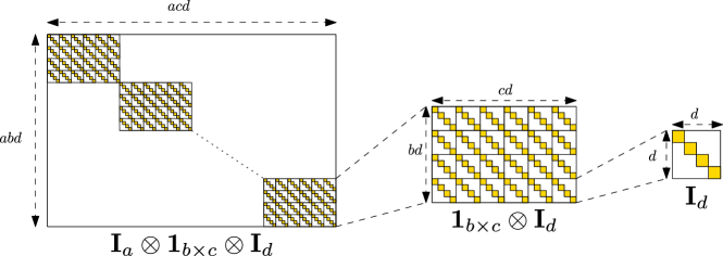
Figure 2: A ${\boldsymbol{\pi}}$-butterfly factor with ${\boldsymbol{\pi}}=(a,b,c,d)$ is a block-diagonal matrix with $a$ blocks, where each block itself is a block matrix composed by $b\times c$ diagonal matrices of size $d\times d$.

A butterfly architecture of depth $L\in\mathbb{N}_{>0}$ is a sequence ${\boldsymbol{\beta}}=({\boldsymbol{\pi}}_{\ell})_{\ell=1}^{L}$ of patterns ${\boldsymbol{\pi}}_{\ell}=(a_{\ell},b_{\ell},c_{\ell},d_{\ell})\in(\mathbb{N}_{>0})^{4}$ satisfying the following compatibility condition: $a_{\ell}c_{\ell}d_{\ell}=a_{\ell+1}b_{\ell+1}d_{\ell+1}$ for $\ell\in\{1,\ldots,L-1\}$. A matrix $\mathbf{W}$ is called a butterfly matrix if there exists a butterfly architecture ${\boldsymbol{\beta}}=({\boldsymbol{\pi}}_{\ell})_{\ell=1}^{L}$ with associated ${\boldsymbol{\pi}}_{\ell}$-butterfly factors $\mathbf{B}_{\ell}$ such that $\mathbf{W}=\mathbf{B}_{1}\dots\mathbf{B}_{L}$.

Therefore, a ${\boldsymbol{\pi}}$-butterfly factor is sparse and structured. It has at most $abcd$ nonzero entries when ${\boldsymbol{\pi}}=(a,b,c,d)$, which yields a sparsity ratio $\frac{abcd}{a^{2}bcd^{2}}=\frac{1}{ad}$, since it is of size $abd\times acd$.

2.1 Generic algorithm for butterfly sparse matrix multiplication

Algorithm 1 is a generic algorithm tailored to the butterfly sparsity, allowing for the multiplication of a batch of vectors with a single ${\boldsymbol{\pi}}$-butterfly factor. It generalizes to general butterfly patterns ${\boldsymbol{\pi}}=(a,b,c,d)$ the one suggested by Dao et al. (2022b) in the specific cases $a=1$ or $d=1$.

Algorithm 1 Butterfly sparse matrix multiplication

1:${\boldsymbol{\pi}}=(a,b,c,d)$, $\mathbf{B}\in\Sigma^{{\boldsymbol{\pi}}}$, $\mathbf{X}\in\mathbb{R}^{K\times N}$ ($N:=acd$)

2:$\mathbf{Y}=\mathbf{X}{\mathbf{B}}^{\top}\in\mathbb{R}^{K\times M}$ ($M:=abd$)

3:$\mathbf{Y}\leftarrow\mathbf{0}_{K\times M}$

4:for $(i,j)\in\llbracket 0,a-1\rrbracket\times\llbracket 0,d-1\rrbracket$ do

5:     $\texttt{col}\leftarrow\left\{i\frac{N}{a}+j+\ell d\,|\,\ell\in\llbracket 0,c-1\rrbracket\right\}$

6:     $\texttt{row}\leftarrow\left\{i\frac{M}{a}+j+kd\,|\,k\in\llbracket 0,b-1\rrbracket\right\}$

7:     ${\mathbf{Y}}[:,\texttt{row}]\leftarrow{\mathbf{X}}[:,\texttt{col}]{{\mathbf{B}}^{\top}}[\texttt{col},\texttt{row}]$

8:end for

Algorithm 2 Equivalent formulation

1:${\boldsymbol{\pi}},\mathbf{X},\tilde{\mathbf{B}}:={\mathbf{P}}^{\top}\mathbf{B}{\mathbf{Q}}^{\top}$ with $\mathbf{B}\in\Sigma^{{\boldsymbol{\pi}}}$, $\mathbf{P}:=(\mathbf{I}_{a}\otimes\mathbf{P}_{b,d})$, $\mathbf{Q}:={(\mathbf{I}_{a}\otimes\mathbf{P}_{c,d})}^{\top}\text{ cf.~{}\eqref{eq:perfect-shuffle-butterfly-pattern}}$

2:$\mathbf{Y}=\mathbf{X}{\mathbf{B}}^{\top}\in\mathbb{R}^{K\times M}$

3:$\tilde{\mathbf{X}}\leftarrow\mathbf{X}{\mathbf{Q}}^{\top}$

4:$\tilde{\mathbf{Y}}\leftarrow\tilde{\mathbf{X}}{\tilde{\mathbf{B}}}^{\top}$

5:$\mathbf{Y}\leftarrow\tilde{\mathbf{Y}}{\mathbf{P}}^{\top}$

Notations. $\mathbf{X}\in\mathbb{R}^{K\times N}$ is the input matrix (batch size $K$, input dimension $N$). $\Sigma^{{\boldsymbol{\pi}}}$ is the set of matrices with butterfly pattern ${\boldsymbol{\pi}}=(a,b,c,d)$ (Definition 2.1). $\mathbf{0}_{m\times n}$ is the $m\times n$ matrix filled with zeros. For integers $a\leq b$, $\llbracket a,b\rrbracket:=\{a,a+1,\ldots,b\}$. For a matrix $\mathbf{M}$, ${\mathbf{M}}[I,:]$ is the submatrix restricted to rows $I$, and ${\mathbf{M}}[I,J]$ is the restriction to rows $I$ and columns $J$. Matrix transposition is represented by $\top$. Matrix indices start at zero.

Theoretical complexity. It is not hard to see that the theoretical complexity of Algorithm 1, defined as the number of scalar multiplications, is $Kabcd$, for a batch size $K$ and a pattern ${\boldsymbol{\pi}}=(a,b,c,d)$.

On Algorithm 1, and the equivalent Algorithm 2. When $d=1$, the butterfly factor $\mathbf{B}$ is block-diagonal with $a$ dense blocks, as can be seen from Figure 2. In this special case, Algorithm 1 loops over each of these blocks, given by ${\mathbf{B}}[\texttt{row},\texttt{col}]$, where the subsets row and col are indexed by $i\in\llbracket 0,a-1\rrbracket$ in Algorithm 1, and performs the matrix multiplication with the corresponding submatrix of $\mathbf{X}$. The general case $d\geq 1$ is similar: the butterfly factor $\mathbf{B}$ is, up to permutation operations, block-diagonal with $ad$ dense blocks, and Algorithm 1 loops over each of these dense blocks, given by ${\mathbf{B}}[\texttt{row},\texttt{col}]$ with row and col defined in lines 5 and 6. See Figure 3 for an illustration. More precisely, for any ${\boldsymbol{\pi}}=(a,b,c,d)$, denoting $\tilde{{\boldsymbol{\pi}}}=(ad,b,c,1)$, we have:

$$\mathbf{S}_{{\boldsymbol{\pi}}}=\underbrace{(\mathbf{I}_{a}\otimes\mathbf{P}_{b,d})}_{:=\mathbf{P}}\underbrace{(\mathbf{I}_{ad}\otimes\mathbf{1}_{b\times c})}_{=\mathbf{S}_{\tilde{{\boldsymbol{\pi}}}}}\underbrace{{(\mathbf{I}_{a}\otimes\mathbf{P}_{c,d})}^{\top}}_{:=\mathbf{Q}}=\mathbf{P}\mathbf{S}_{\tilde{{\boldsymbol{\pi}}}}\mathbf{Q},$$ (1)

where $\mathbf{P}_{p,q}$ for two integers $p,q$ is the so-called $(p,q)$ perfect shuffle permutation matrix of size $pq\times pq$ (Van Loan, 2000) (see Section C.1 for details). Therefore, for any $\mathbf{B}\in\Sigma^{{\boldsymbol{\pi}}}$, we have $\mathbf{B}=\mathbf{P}\tilde{\mathbf{B}}\mathbf{Q}$ with $\tilde{\mathbf{B}}:={\mathbf{P}}^{\top}\mathbf{B}{\mathbf{Q}}^{\top}\in\Sigma^{\tilde{{\boldsymbol{\pi}}}}$, i.e., $\tilde{\mathbf{B}}$ is block-diagonal with $ad$ dense blocks of size $b\times c$. Algorithm 1 loops over each of the $ad$ dense submatrices ${\mathbf{B}}[\texttt{row},\texttt{col}]$ and accumulates the result in $\mathbf{Y}$. Many concrete implementations of Algorithm 1 presented below are based on the equivalent formulation $\mathbf{Y}=\mathbf{X}{\mathbf{B}}^{\top}=\mathbf{X}{\mathbf{Q}}^{\top}{\tilde{\mathbf{B}}}^{\top}{\mathbf{P}}^{\top}$: they directly store ${\tilde{\mathbf{B}}}^{\top}$ instead of ${\mathbf{B}}^{\top}$, permute the inputs with $\mathbf{Q}$, multiply with ${\tilde{\mathbf{B}}}^{\top}$, and repermute with $\mathbf{P}$, which corresponds to Algorithm 2.

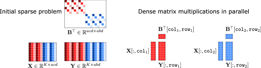
Figure 3: Illustration of Algorithm 1 for sparsity pattern ${\boldsymbol{\pi}}=(2,3,2,3)$ and batch size $K=8$. The subsets of rows and columns $(\texttt{row}_{1},\texttt{col}_{1})$ are associated with the values $(i,j)=(0,1)$ in the “for" loop of Algorithm 1, whereas $(\texttt{row}_{2},\texttt{col}_{2})$ are associated with $(i,j)=(1,1)$.

2.2 Baseline GPU implementations

We now describe concrete baseline GPU implementations of Algorithms 1 and 2. The exact codes are given in Section D.1.

bmm and bsr implementations. We consider the bmm implementation from Dao et al. (2022b), and we also propose a new implementation bsr. Note that the original bmm implementation from Dao et al. (2022b) only works for a pattern ${\boldsymbol{\pi}}=(a,b,c,d)$ satisfying $a=1$ or $d=1$. We extend it to the general case. Both bmm and bsr implement Algorithm 2 as specified by Table 1. For the multiplication with $\tilde{\mathbf{B}}$ (line 4 in Algorithm 2), bmm relies on batched GEMM NVIDIA routines called through torch.bmm, while bsr relies on the PyTorch block-sparse library.

	bmm	bsr
Storage format for $\tilde{\mathbf{B}}$	3D-tensor of shape $(ad,b,c)$	2D-tensor of shape $(abd,acd)$ stored in BSR format
Line 3 of Algorithm 2	torch.reshape
Line 4 of Algorithm 2	torch.bmm	torch.nn.functional.linear
Line 5 of Algorithm 2	torch.reshape

Table 1: Differences in the implementation of Algorithm 2 between bmm and bsr.

einsum implementation. We propose a new baseline implementing Algorithm 1 with tensor contractions, using the einops library (Rogozhnikov, 2021). It stores the nonzero entries of $\mathbf{B}\in\Sigma^{{\boldsymbol{\pi}}}$ with a 4D-tensor B_einsum of shape $(a,b,c,d)$, in such a way that the slice $\texttt{B\_einsum}[i,:,:,j]$ for $(i,j)\in\llbracket 0,a-1\rrbracket\times\llbracket 0,d-1\rrbracket$ stores the entries of ${\mathbf{B}}[\texttt{row},\texttt{col}]$ where row, col are defined in lines 5 and 6 of Algorithm 1. The batched matrix multiplication operations at line 7 are then implemented using Einstein summation between this 4D-tensor and a reshaped input tensor.

The above implementations (bmm, bsr, einsum) can be compared to the two following generic implementations (dense and sparse) that ignore the butterfly sparsity.

dense implementation. This ignores the sparsity of the butterfly factor $\mathbf{B}$, by storing all its entries, including zeros, in a tensor of shape $(M,N)$. The multiplication is done with torch.nn.functional.linear, the default PyTorch implementation for linear layers.

sparse implementation. This exploits the sparsity of the butterfly factor $\mathbf{B}$ but not its structure (recall that the sparsity pattern is not arbitrary, but structured as Kronecker products, see Definition 2.1). The nonzero entries of the factor $\mathbf{B}$ are saved in a tensor stored in the Compressed Sparse Row (CSR) format, and the matrix multiplication is done with torch.nn.functional.linear.

Batch-size-first vs. batch-size-last. The entries of the input $\mathbf{X}\in\mathbb{R}^{K\times N}$ can be stored either in a PyTorch tensor X_bsf of shape $(K,N)$, or in a PyTorch tensor X_bsl of shape $(N,K)$, in such a way that the entries of the row ${\mathbf{X}}[k,:]$ are stored in the slices $\texttt{X\_bsf}[k,:]$ and $\texttt{X\_bsl}[:,k]$. Because of PyTorch’s row-major convention, the tensor X_bsf stores in contiguous memory the entries of each row ${\mathbf{X}}[k,:]$, as opposed to X_bsl that store contiguously the entries of each column ${\mathbf{X}}[:,i]$. These two different memory layouts are called batch-size-first and batch-size-last in this paper. Note that the tensor saving the output $\mathbf{Y}=\mathbf{X}{\mathbf{B}}^{\top}$ will always be in the same memory layout as the input tensor. All the implementations above can be implemented in both ways. While the main point of the paper is to compare the implementations, we will also study the effect of this memory layout convention.

3 Memory accesses in baseline implementations

While it is not clear what the tensor contraction einsum implementation is exactly doing underneath, the implementations bmm and bsr explicitly perform permutation operations corresponding to $\mathbf{P}$ and $\mathbf{Q}$ (lines 3 and 5 in Algorithm 2) to be able to use high-performance multiplication routines for the multiplication with $\tilde{\mathbf{B}}$ (line 4 in Algorithm 2). This paper assesses for the first time the cost of these memory operations in practice, as we now discuss.

Importance of data transfers. GPU memory management plays a critical role in optimizing performance. Memory in a GPU is organized hierarchically, with global memory being the largest and slowest, followed by shared memory, and finally registers, which are the smallest and fastest (NVIDIA, 2024, Sec. 2.3). By default, data resides in the global memory of the GPU. Each thread of the GPU runs a kernel that reads data from global memory into registers, performs register-level computations, and writes the results back to global memory. Therefore, when operations are bottlenecked by memory accesses, it is critical to minimize data transfers between global memory, shared memory, and registers to obtain an efficient GPU implementation (NVIDIA, 2024, Sec. 5.3).

Data transfers in baseline implementations. In this paper, we argue that the baseline bmm, bsr and einsum implementations for butterfly multiplication require performing several passes between global memory and registers that can account for a large proportion of the total runtime in practice. This suggests that there is room for improvement in the memory accesses of these implementations.

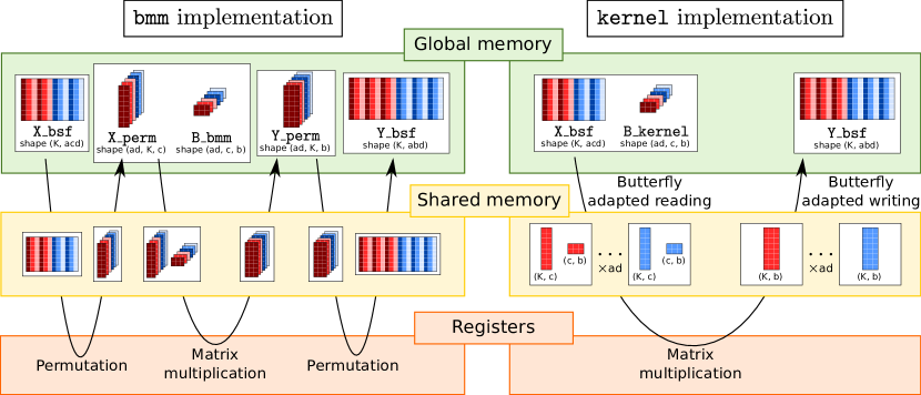
Figure 4: Data flow between the different levels of GPU memory for the bmm implementation (Section 2.2) from Dao et al. (2022b) and the new kernel (Section 4).

Let us focus on bmm, as we will find it to be faster than einsum and bsr. The data flow of bmm is illustrated in Figure 4. There is one pass between the global memory and the registers to perform the permutation with $\mathbf{P}$ (line 5 in Algorithm 2), one for the multiplication with $\tilde{\mathbf{B}}$ (line 4), and another one for the permutation with $\mathbf{Q}$ (line 3).

Doing at least three passes between the global memory and the registers is necessary for any implementation that performs all the multiplications ${\mathbf{X}}[:,\texttt{col}]{{\mathbf{B}}^{\top}}[\texttt{col},\texttt{row}]$ (line 7 in Algorithm 1, or equivalently line 4 in Algorithm 2) by calling high-performance libraries from common Python interfaces (PyTorch, Tensorflow). Indeed, calling multiplication routines from Python requires in general having the entries of ${\mathbf{X}}[:,\texttt{col}]$ and ${{\mathbf{B}}^{\top}}[\texttt{col},\texttt{row}]$ stored contiguously in global memory. This is not the case of the entries of ${\mathbf{X}}[:,\texttt{col}]$ when $\mathbf{X}\in\mathbb{R}^{K\times N}$ is directly stored contiguously in a 2D-tensor of shape $(K,N)$ or $(N,K)$, and when $d>1$, because the indices in col are equally spaced by $d$ (see line 6 in Algorithm 2). And this is the only memory layout that we can assume for the entries of $\mathbf{X}$ when the matrix multiplication is a part of a larger pipeline, such as in a neural network. Therefore, a first pass between the global memory and the registers is required to write the entries of ${\mathbf{X}}[:,\texttt{col}]$ contiguously in global memory, see Figure 4. Similarly, the result of the multiplication ${\mathbf{Y}}[:,\texttt{row}]={\mathbf{X}}[:,\texttt{col}]{{\mathbf{B}}^{\top}}[\texttt{col},\texttt{row}]$, as returned by an efficient routine called from Python, will in general be stored contiguously in global memory for each pair $(\texttt{row},\texttt{col})$. But indices in row are equally spaced by $d$: this requires another pass to rewrite them equally spaced by $d$ in the final output 2D-tensor storing all the entries of $\mathbf{Y}$ contiguously in memory. With the pass implied by the actual multiplication routine, this results in three passes between the global memory and the registers (Figure 4).

Estimated time for memory rewritings in bmm. To the best of our knowledge, this paper is the first to discuss the practical cost of memory rewritings in baseline implementations such as bmm. For input and output dimensions $N$ and $M$, and a batch size $K$, the memory rewritings of ${\mathbf{X}}[:,\texttt{col}]$ and ${\mathbf{Y}}[:,\texttt{row}]$ for all pairs $(\texttt{row},\texttt{col})$ (Algorithm 1) concern $KN+KM$ coefficients to be moved in memory: each coefficient of the input and output tensors is moved exactly once. The total number of scalar multiplications performed when computing the products ${\mathbf{Y}}[:,\texttt{row}]={\mathbf{X}}[:,\texttt{col}]{{\mathbf{B}}^{\top}}[\texttt{col},\texttt{row}]$ for all $(\texttt{row},\texttt{col})$ (Algorithm 1) is equal to $K\times\textrm{\#nnz}$ (batch size times the number of nonzero in $\mathbf{B}$).

Figure 5 reports time estimates for memory rewritings in the bmm implementation (see Section B.2 for more details on the experimental protocol). It shows that the relative time spent on memory rewritings increases with the ratio

$$\frac{\texttt{number of memory rewritings}}{\texttt{number of scalar multiplications}}=\frac{KN+KM}{K\times\textrm{\#nnz}}=\frac{b+c}{bc}$$ (2)

where the last equality holds in the case of a butterfly factor with sparsity pattern ${\boldsymbol{\pi}}=(a,b,c,d)$, since $N=acd$, $M=abd$ and $\textrm{\#nnz}=abcd$ in this case. Figure 5 shows that these memory rewritings can take up to ${45}\%$ of the total runtime. In conclusion, it is crucial to optimize the data transfers between the different levels of GPU memory to improve current implementations.

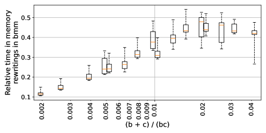
Figure 5: Estimated relative time spent on memory rewritings in bmm for the multiplication with $\mathbf{B}\in\Sigma^{{\boldsymbol{\pi}}}$, for several ${\boldsymbol{\pi}}=(a,b,c,d)$. We regroup patterns by their value of $(b+c)/(bc)$, and plot a boxplot to summarize the corresponding measurements.

4 New CUDA kernel with reduced memory transfers

For better management of memory accesses, we need to go to a lower level than Python. This is where the new CUDA kernel comes in. It has the minimum possible number of back and forth between global memory and registers thanks to custom read and write phases between global and shared memory, tailored to butterfly sparsity. These new read and write phases allow to perform a single back and forth between the different levels of memory, as shown in Figure 4.

Implementation. The reading phase loads the entries of ${\mathbf{X}}[:,\texttt{col}]$ directly from the global memory by accessing non-contiguous columns of $\mathbf{X}$ equally spaced by $d$ (see Figure 3), and stores them contiguously in shared memory. Since we are still loading entire columns of $\mathbf{X}$, the reading phase is expected to be more efficient if the entries in the same column are contiguous in memory, in order to ensure that most of the memory accesses remain contiguous and efficient. This will only be the case when $\mathbf{X}$ is stored with the batch-size-last memory layout (as defined in Section 2.2). When in shared memory, the kernel implements the classic tile matrix multiplication algorithm (Li et al., 2019; Boehm, 2022; NVIDIA, 2023a, b, 2024) to compute each product ${\mathbf{X}}[:,\texttt{col}]{{\mathbf{B}}^{\top}}[\texttt{col},\texttt{row}]$ for each subsets row, col in Algorithm 1. Once these products are computed, the kernel again has a custom writing phase from shared to global memory, rewriting the results that are stored contiguously in shared memory, to non-contiguous locations in global memory, because each submatrix ${\mathbf{Y}}[:,\texttt{row}]$ corresponds to non-consecutive columns of the output $\mathbf{Y}$ (see Figure 3). This writing phase is also expected to be more efficient in the batch-size-last memory layout, ensuring the entries of a same column of ${\mathbf{Y}}[:,\texttt{row}]$, and thus the write operations, to be contiguous in memory.

Comparison with other baseline implementations. This new kernel has fewer global memory accesses compared to the baselines einsum, bsr and bmm, because it only reads each coefficient of $\mathbf{X}$ and $\mathbf{B}$ once and writes the result of the multiplication $\mathbf{Y}$ once, while those baseline implementations read $\mathbf{X}$ and $\mathbf{Y}$ twice and rewrite them once (to permute them). It also has fewer global memory accesses compared to the dense implementation (Section 2.2), since the dense implementation also reads the zero entries of $\mathbf{B}$ and the corresponding coefficients of $\mathbf{X}$, while our kernel does not. Compared to the generic sparse implementation, we have the same number of memory accesses, but the sparse implementation is agnostic to the sparsity structure of $\mathbf{B}$, so it is expected to be less efficient since the memory accesses are not tailored to the known location of the nonzero entries.

5 Benchmarking the multiplication by a single butterfly factor

We perform the first benchmark of different implementations for butterfly matrix multiplication, at the finest granularity, where we measure the time for the multiplication with a single butterfly factor $\mathbf{B}$. In particular, we validate numerically the benefits of reducing the memory transfers in the kernel implementation, compared to the baselines einsum, bsr and bmm.

Protocol. The benchmark is run in float-precision on a subset of $600$ sparsity patterns ${\boldsymbol{\pi}}=(a,b,c,d)$ in $\alpha\times\beta\times\beta\times\alpha$, with $\alpha:=\{1,2,3,4,6,8,12,16,24,32,48,64,96,128\}$, $\beta:=\{48,64,96,128,192,256,384,512,768,1024\}$, such that $b=c$ or $b=4c$ or $c=4b$. These patterns correspond to dimensions of butterfly factors $\mathbf{B}\in\mathbb{R}^{M\times N}$ with $(M,N)=(abd,acd)$ that could be used in neural networks. We choose as batch size $K=128\times 196=25088$, which is standard as it corresponds to the effective batch size for linear layers in ViTs where the number of sequences per batch is $128$, and the number of tokens per sequence is $196$. Further details are given in Section B.1.

Table 2: Percentage out of $600$ patterns $(a,b,c,d)$ where algo1 is faster than the algo2 (denoted by $\text{time}(\texttt{algo1})<\text{time}(\texttt{algo2})$), and the median acceleration factor in such cases (that is, the median ratio $\frac{\textrm{time of }\texttt{algo2}}{\textrm{time of }\texttt{algo1}}$). For each implementation, we take the minimum time between the batch-size-first and the batch-size-last memory layout.

$\text{min time}\begin{pmatrix}{\texttt{kernel}}{}\\ {\texttt{bmm}}{}\\ {\texttt{einsum}}{}\\ {\texttt{bsr}}{}\end{pmatrix}<\text{min time}\begin{pmatrix}{\texttt{dense}}{}\\ {\texttt{sparse}}{}\end{pmatrix}$	$\text{time}({\texttt{bmm}}{})<\text{min time}\begin{pmatrix}{\texttt{einsum}}{}\\ {\texttt{bsr}}{}\\ {\texttt{dense}}{}\\ {\texttt{sparse}}{}\end{pmatrix}$	$\text{time}({\texttt{kernel}}{})<\text{min time}\begin{pmatrix}{\texttt{bmm}}{}\\ {\texttt{einsum}}{}\\ {\texttt{bsr}}{}\\ {\texttt{dense}}{}\\ {\texttt{sparse}}{}\end{pmatrix}$
${99.67}\%$ $(\times 6.57)$	${92.66}\%$ $(\times 1.37)$	${88.10}\%$ $(\times 1.39)$

Implementations specialized to butterfly sparsity improves over generic implementations. The first line of Table 2 shows that at least one of the implementations specialized to the butterfly structure among kernel, bmm, einsum and bsr improves over the generic dense and sparse implementation, which do not take into account the butterfly sparsity. The speedup increases with the matrix size, see Section B.3.

The baseline bmm is faster than the other baselines einsum and bsr. This is shown in the second line of Table 2, where the bmm implementation improves over $\min({\texttt{einsum}}{},{\texttt{bsr}}{})$ in ${93}\%$ of the tested cases. The speedup increases with the matrix size, see Section B.4. Therefore, when comparing the new kernel implementation to other baselines, we will mainly focus on the comparison between bmm and kernel.

The new kernel implementation is faster than existing baselines. The third row of Table 2 shows that kernel is faster than all other baselines in ${88}\%$ of the tested patterns. This empirically validates the benefits of the reduced memory transfer in the kernel implementation. In the following, we provide further details on the influence of the memory layout (batch-size-first vs. batch-size-last) on this improvement. Additionally, we analyze the patterns ${\boldsymbol{\pi}}=(a,b,c,d)$ for which the kernel outperforms baseline implementations.

Figure 6: Time speedup factor of kernel compared to $\min({\texttt{bmm}}{},{\texttt{einsum}}{},{\texttt{bsr}}{})$. For each implementation, we take the minimum time between the batch-size-first and batch-size-last memory layouts. We regroup the patterns by their value of $(b+c)/(bc)$, and plot a boxplot to summarize the corresponding measurements.

Figure 7: Energy consumed by kernel compared to the minimum consumed by bmm, einsum and bsr. For each implementation, we take the minimum energy consumed between the batch-size-first and batch-size-last memory layouts. We regroup patterns by their value of $d(b+c)/(bc)$.

Impact of the memory layout. For baseline implementations, switching to batch-size-last yields a high systematic speedup for sparse, high variability in the speedup of bsr, and essentially no impact to negative impact for the other methods, see Section B.5 for numerical results. The important part is that it has no impact on bmm, and since bmm is the fastest baseline implementation (Table 2), switching to batch-size-last has no impact on the best of the baseline implementations. However, it yields a systematic speedup (about $\times 2$) for the kernel implementation. This acceleration is expected, since the batch-size-last memory layout allows for more efficient memory accesses in the kernel implementation, as detailed in Section 4.

Analyzing the cases where kernel outperforms baselines. As seen in Section 4, the kernel has an improved memory access design compared to the rest of the baselines. Figure 6 confirms this experimentally: the kernel implementation becomes increasingly time-efficient compared to the baseline implementations as the relative number of memory accesses increases, i.e. when the following ratio increases (introduced in (2))

$$\frac{\texttt{number of memory rewritings}}{\texttt{number of scalar multiplications}}=(b+c)/(bc).$$

The kernel improves on energy efficiency. For sparsity patterns ${\boldsymbol{\pi}}=(a,b,c,d)$, the integer $d$ corresponds to the distance between two columns of the butterfly factor with the same set of nonzero entries. When $d$ is large, the memory rewritings made by bmm are likely to be more expensive as the columns in the same set col of Algorithm 1 are further away from each other. In practice, we observe the kernel to be more and more energy-efficient as the relative number of memory rewritings $(b+c)/bc$ times the cost $d$ of these memory rewritings increases, as shown in Figure 7. Overall, the median energy reduction factor is $\times 0.85$, and the new kernel improves the energy consumption in ${72}\%$ of the tested cases. See Section B.1 for details about the measurements. This is particularly noteworthy as it demonstrates that the kernel not only achieves higher time efficiency but also reduces energy consumption compared to other baselines. This dual advantage makes the kernel an effective solution for improving both performance and sustainability.

6 Broader implications for neural networks: accelerating inference

The inference of neural networks is claimed to represent 90% of the cost of machine learning at scale according to independent reports from both NVIDIA (HPCwire, 2019) and Amazon Web Services (Jeff Barr, 2019). We now investigate whether replacing fully-connected layers by butterfly matrices accelerates the inference. While the same could also apply to other architectures, we will consider Vision Transformers (ViTs) (Dosovitskiy et al., 2020). We find that the computational cost of fully-connected layers is significant in such architectures: depending on the size of the ViT, from $30\%$ to $60\%$ of the total time in a forward pass is spent in fully-connected layers (see Section B.6 for details).

Protocol. We benchmark in float-precision various components of a ViT-S/16 architecture: a linear layer with bias, an MLP with non-linear activation and/or normalization layers, a multi-head attention module, etc. As in Dao et al. (2022b), the matrices that are replaced by a butterfly matrix are the weight matrices of linear layers in feed-forward network modules, and the projection matrices for keys, queries and values in multi-head attention modules. We focus on batch-size-first as it is the default convention in PyTorch. Details and some additional results are given in Section B.7.

Results. We denote by $\text{time}(\texttt{fully-connected})$ the inference time without butterfly matrices (and therefore, with the standard PyTorch implementation). Table 3 shows that $\text{time}({\texttt{kernel}}{})<\text{time}({\texttt{bmm}}{})<\text{time}(\texttt{fully-connected})$ over all the different submodules. This concretely shows that using butterfly matrices and the kernel implementation accelerates the inference of standard neural networks.

Table 3: Acceleration of submodules of a ViT-S/16 using butterfly matrices.

	$\frac{\text{time}({\texttt{bmm}}{})}{\text{time}(\texttt{fully-connected})}$	$\frac{\text{time}({\texttt{kernel}}{})}{\text{time}(\texttt{fully-connected})}$
Linear $N\times N$	$0.82$	0.50
Feed-forward network	$0.91$	0.77
Multi-head attention	$0.87$	0.79
Block	$0.90$	0.78
Butterfly ViT-S/16	$0.89$	0.78

7 Conclusion

This work is the first to evaluate the efficiency of existing butterfly sparse matrix multiplication algorithms on the GPU. Our benchmark shows that baseline implementations require costly memory rewrites in global memory, which are not negligible in practice. The proposed new CUDA kernel significantly reduces the cost of global memory accesses. Specifically, this new kernel is faster than previous baseline implementations, with a median reduction factor of $\times 0.85$. We also show how it can be used to accelerate the inference of neural networks.

Perspectives. While we have focused on optimizing memory management, the multiplication part of our kernel may still have room for improvement, especially in half-precision. We hope this will encourage work in that direction. The new kernel is particularly performant in batch-size-last. We hope this will lead to further efforts in the batch-size-first setting and encourage revisiting other common operations in neural networks within the batch-size-last configuration. A translation of our kernel into OpenCL could enable it to run on AMD hardware and other platforms. We also hope that our benchmark will serve as a baseline for comparing butterfly implementations on other hardware: CPU, Intelligence Processing Unit, FPGA, etc.

Acknowledgments

This work was supported in part by the AllegroAssai ANR-19-CHIA-0009, by the NuSCAP ANR-20-CE48-0014 projects of the French Agence Nationale de la Recherche and by the SHARP ANR project ANR-23-PEIA-0008 in the context of the France 2030 program.

The authors thank the Blaise Pascal Center for the computational means. It uses the SIDUS (Quemener and Corvellec, 2013) solution developed by Emmanuel Quemener.

We would also like to thank Patrick Pérez, Gilles Puy, Elisa Riccietti, Nicolas Brisebarre, and Rémi Gribonval for their useful feedback, and Emmanuel Quemener for reserving computing resources for us while we ran our experiments.

Appendices

Appendix A Related works

We now review the numerical results we found in the literature about time efficiency of existing algorithms for sparse butterfly matrix multiplication.

It is reported in Dao et al. [2022b] that some butterfly networks were twice faster to train than their dense counterparts for image classification and language modeling, without additional information.

In Fu et al. [2023] is reported an acceleration of $\mathbf{X}\mapsto\mathbf{W}^{-1}(\mathbf{K}\odot\mathbf{W}\mathbf{X})$ where $\mathbf{K}$ is some dense weight matrix, $\odot$ is the element-wise multiplication, and $\mathbf{W}$ is the DFT matrix (which admits a butterfly factorization), as soon as the dimensions of $\mathbf{W}$ are at least equal to $4096$.

These results do not provide extensive information on the efficiency of sparse butterfly matrix multiplication, motivating the benchmark in this paper.

Appendix B Experiments

B.1 Details on the experiments

The pytorch package version is 2.2 and pytorch-cuda is 12.1.

Matrix sizes. In all our experiments with matrices, we set the batch size to $K=128\times 196=25088$, a very standard choice for ViTs, as this quantity corresponds to the standard number of tokens per sequence (192) multiplied by the standard number of sequences in a batch of inputs (128). When dealing with a batch of images in neural networks, we choose the standard choice of batch size $K=128$.

Matrix entries. The coordinates of any butterfly factor $\mathbf{B}\in\mathbb{R}^{abd\times acd}$ with sparsity pattern $(a,b,c,d)$ are drawn i.i.d. uniformly in $[-\frac{1}{\sqrt{c}},\frac{1}{\sqrt{c}}]$, as for the initialization chosen for training in Dao et al. [2022b], while the coordinates of the inputs $\mathbf{X}$ are drawn i.i.d. according to a standard normal distribution $\mathcal{N}(0,1)$.

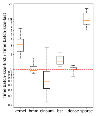
Figure 17: Boxplots of the ratio $\frac{\text{time of {\em batch-size-first}{}}}{\text{time of {\em batch-size-last}{}}}$ in half-precision.

Benchmarking time execution. All the experiments measuring the time execution of the implementations (Tables 2, 3, 4 and 7, Figures 5, 6, 15, 10, 11, 16, 13, 6, 12, 17, 14 and 9) are done on a single NVIDIA A100-PCIE-40GB GPU on an Intel(R) Xeon(R) Silver 4215R CPU @ 3.20GHz with 377G of memory. The full benchmark took approximately 3 days in an isolated environment, ensuring that no other processes were running concurrently.

Measurements are done using the PyTorch tool torch.utils.benchmark.Timer. The medians are computed on at least 10 measurements of 10 runs. In ${94.2}\%$ of the cases, we have an interquartile range (IQR) that is at least 100 times smaller than the median (resp. ${98}\%$ for 50 times smaller, and ${99.7}\%$ for 10 times smaller).

Benchmarking energy consumption. Measurements of the energy consumption (Figure 7) is done on a single NVIDIA Tesla V100-PCIE-16GB GPU on an Intel(R) Xeon(R) Silver 4215R CPU @ 3.20GHz with 754G of memory. The full benchmark took approximately 1.5 days in an isolated environment. Measurements are made using the pyJoules software toolkit. The medians are computed on at 10 measurements of at least 16 runs. In ${96}\%$ of the cases, the IQR is at least 10 times smaller than the median, and in all the cases, it is 5 times smaller.

Patterns benchmarked for time measurements (Section 5). The considered patterns are generated by the Python code written in Figure 8. In all the cases, we only consider patterns $(a,b,c,d)$ with $b=c$ or $b=4c$ or $c=4d$ to have an input size $N$ and an output size $M$ such that $N=M$ or $N=4M$ or $M=4N$. This choice is motivated by the fact that fully-connected layers in ViTs satisfy have input and output sizes satisfying these constraints.

The first "for" loop in Figure 8 generates a wide range of patterns $(a,b,c,d)$ with $a=1$, as this represents the simplest scenario. Indeed, the case $a>1$ simply corresponds to the case $a=1$ but repeated $a$ times in parallel.

The second "for" loop in Figure 8 generates patterns with $a>1$ offering fewer choices for $d$ to keep the benchmark concise in terms of execution time. This loop also imposes additional conditions on $b$ and $c$ (line 28 of the code) that we now explain. Many graphs are plotted based on the ratio $(b+c)/bc$, as introduced in Equation 2. Because of that, our goal was to include as many distinct ratios $(b+c)/bc$ as possible while keeping the benchmark brief. We excluded certain $(b,c)$ values because they resulted in a ratio that was very close to one already in the benchmark and were more computationally intensive.

⬇

1import itertools

2

3batch_size = 25_088

4size_limit = 2_147_483_647

5

6a_list = [1, 2, 3, 4, 6, 8, 12, 16, 24, 32, 48, 64, 96, 128]

7b_list = [48, 64, 96, 128, 192, 256, 384, 512, 768, 1024]

8c_list = [48, 64, 96, 128, 192, 256, 384, 512, 768, 1024]

9d_list1 = [1, 2, 3, 4, 6, 8, 12, 16, 24, 32, 48, 64, 96, 128]

10d_list2 = [4, 16, 64]

11

12def get_patterns_benchmark():

13 patterns_list = []

14

15 def add_pattern(a, b, c, d):

16 if batch_size * a * c * d <= size_limit and \

17 batch_size * a * b * d <= size_limit and \

18 a * b * c * d <= size_limit:

19 patterns_list.append((a, b, c, d))

20

21 for b, c, d in itertools.product(b_list, c_list, d_list1):

22 a = 1

23 if (b == c or b == 4 * c or c == 4 * b):

24 add_pattern(a, b, c, d)

25

26 for a, b, c, d in itertools.product(a_list, b_list, c_list, d_list2):

27 if a != 1 and \

28 (b, c) not in [(1024, 256), (256, 1024), (128, 512), (512, 128), (64, 256), (256, 64)] and \

29 (b == c or b == 4 * c or c == 4 * b):

30 add_pattern(a, b, c, d)

31

32 return patterns_list

Figure 8: Python code to generate the patterns benchmarked for the execution time in the numerical experiments of Section 5.

Patterns benchmarked for energy measurements (Section 5). For the energy measurements, the goal is to have diverse sparsity patterns $(a,b,c,d)$ corresponding to many different ratios $d(b+c)/bc$ to observe the trend in Figure 7, while keeping the benchmark as short as possible. We chose to consider the cartesian product of

⬇

1a_list = [1, 4, 16, 32, 64]

2b_list = [48, 64, 96, 128, 192, 256, 384, 512, 768, 1024]

3c_list = [48, 64, 96, 128, 192, 256, 384, 512, 768, 1024]

4d_list = [1, 2, 3, 4, 6, 8, 12, 16, 24, 32, 48, 64]

by skipping as in Figure 8 all the patterns with

⬇

1(b,c) in [(1024 , 256) , (256 , 1024) , (128 , 512) , (512 , 128) , (64 , 256) , (256 , 64)]

and also all the patterns such that

⬇

1 b != c and b != 4 * c and c != 4 * b

for the same reasons as the ones explained above in the case of the benchmark on the time execution.

Details on boxplots. In all boxplots (Figures 5, 6, 15, 10, 11, 16, 13, 6, 12, 17, 14, 9 and 7), the orange line corresponds to the median, the boxes to the first and third quartile and the whiskers to the 5th and the 95th percentile. Outliers are not represented on the graph.

B.2 Estimating the time for memory rewritings in the bmm implementation (Section 3)

Protocol. Given a pattern ${\boldsymbol{\pi}}=(a,b,c,d)$ and an input $\mathbf{X}\in\mathbb{R}^{K\times acd}$ for some batch size $K$, we first measure the time $\Delta t$ to compute $\mathbf{Y}:=\mathbf{X}{\mathbf{B}}^{\top}$ using the bmm implementation. Then, we measure the time $\Delta\tilde{t}$ to perform only the multiplication operations ${\mathbf{Y}}[:,\texttt{row}]={\mathbf{X}}[:,\texttt{col}]{{\mathbf{B}}^{\top}}[\texttt{col},\texttt{row}]$ in the bmm implementation (line 4 of Algorithm 2). Therefore, the estimated relative time to perform the memory rewritings of lines 3 and 5 of Algorithm 2 is simply $\frac{\Delta t-\Delta\tilde{t}}{\Delta t}$.

Results. Figure 5, which is replicated in the left part of Figure 9, shows that the relative time spent doing memory rewritings in bmm increases with the ratio $(b+c)/(bc)$, in the batch-size-first memory layout. Figure 9 shows that this is similar for both batch-size-first and batch-size-last.

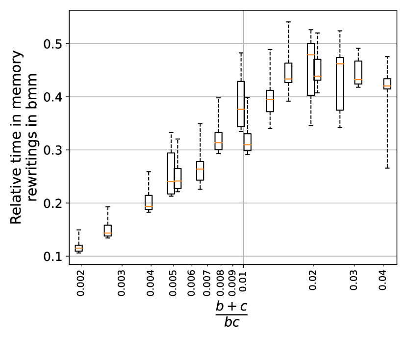
(a) Batch-size-first (same as Figure 5).

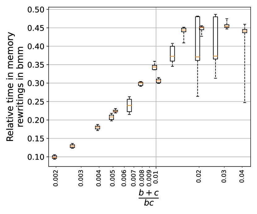
(b) Batch-size-last.

Figure 9: Estimated relative time spent on memory rewritings in bmm for the multiplication with $\mathbf{B}\in\Sigma^{{\boldsymbol{\pi}}}$, for several ${\boldsymbol{\pi}}=(a,b,c,d)$. We regroup patterns by their value of $(b+c)/(bc)$, and plot a boxplot to summarize the corresponding measurements.

B.3 Details on min time(kernel, bmm, bsr, einsum) vs. min time(dense, sparse) (Section 5)

Figure 10 shows that the speed-up factor of implementations specialized to the butterfly sparsity (kernel, bmm, bsr, einsum) over the generic dense and sparse implementations increases with the matrix size $M\times N$. We recall that $M=acd$ and $N=abd$ for a butterfly factor with pattern ${\boldsymbol{\pi}}=(a,b,c,d)$.

B.4 Details on time(bmm) vs. min time(bsr, einsum) (Section 5)

Figure 11 shows that for a sufficient large matrix size $M\times N$, we always have time(bmm) $<$ min time(bsr, einsum), i.e., the bmm implementation is the most efficient among all baseline implementations (bmm, einsum, bsr).

Figure 10: Speed-up factor of min time(kernel, bmm, bsr, einsum) compared to min time(dense, sparse) as a function of the matrix size $M\times N$.

Figure 11: Speed-up factor of time(bmm) compared to min time(einsum, bsr) as a function of the matrix size $M\times N$.

B.5 Details on the impact of the memory layout (Section 5)

Figure 12 shows the impact of the memory layout on the execution time of each implementation.

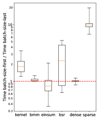
Figure 12: Boxplots of the ratio $\frac{\text{time of {\em batch-size-first}{}}}{\text{time of {\em batch-size-last}{}}}$.

Table 4 shows the percentage of patterns for which the kernel implementation improves over all baseline implementations, either in the batch-size-first or the batch-size-last memory layout. When restricting all implementations to the batch-size-first layout, the kernel still improves on ${20}\%$ of the tested patterns despite non-contiguous memory accesses (Section 4).

Table 4: Percentage out of $600$ patterns $(a,b,c,d)$ where algo1 is faster than the algo2 (denoted by $\text{time}(\texttt{algo1})<\text{time}(\texttt{algo2})$), and the median acceleration factor in such cases (that is, the median ratio $\frac{\textrm{time of }\texttt{algo2}}{\textrm{time of }\texttt{algo1}}$).

	$\text{time}({\texttt{kernel}}{})<\text{min time}({\texttt{bmm}}{},{\texttt{einsum}}{},{\texttt{bsr}}{},{\texttt{dense}}{},{\texttt{sparse}}{})$
Batch-size-first	${20.0}\%$ ($\times 1.28$)
Batch-size-last	${88.1}\%$ ($\times 1.39$)

B.6 Time spent in linear layers in vision transformers

This section gives a numerical lower bound estimate on the time spent in fully-connected layers in a Vision Transformer (ViT).

Results. Table 5 shows that, for different ViTs, the fraction of computation time solely dedicated to linear layers in feed-forward network modules varies between ${31}\%$ and ${53}\%$ in half-precision, and ${46}\%$ and ${61}\%$ in float-precision. This proportion increases with the size of the architecture. This shows that a non-negligible amount of ViTs inference is dedicated to fully-connected layers. Note that the time for the fully-connected linear layers in the multi-head attention module is not included in our measurements, so our estimate is only a lower bound on the time effectively devoted to all fully-connected layers in transformer architectures.

Table 5: Median execution times (ms) of the forward pass in a ViT, and the forward pass in an MLP containing only all the linear layers involved in the feed-forward network modules of the ViT. The latter is reported with its ratio over the first. FP16 is half-precision, FP32 is float-precision.

Architecture	fp16 (s)		fp32 (s)
	Complete	Linear in FFNs	Complete	Linear in FFNs
ViT-S/16	0.014	0.0046 (${31}\%$)	0.090	0.04 (${46}\%$)
ViT-B/16	0.036	0.015 (${42}\%$)	0.30	0.16 (${54}\%$)
ViT-L/16	0.11	0.050 (${46}\%$)	1.0	0.58 (${58}\%$)
ViT-H/14	0.31	0.16 (${53}\%$)	2.6	1.6 (${61}\%$)

Details on the estimation. The transformer architecture is composed of a sequence of transformer blocks, where each block contains a multi-head attention module and a feed-forward network module. The feed-forward network module is an MLP with one hidden layer of neurons, involving two fully-connected linear layers. Table 5 reports the time to perform sequentially all the fully-connected linear layers (without biases) appearing in feed-forward network modules of the considered ViT. This is compared to the total forward time of the transformer network. This is expected to yield a lower bound since we did not measure the time spent in fully-connected linear layers in the multi-head attention module.

Experimental settings. The architecture ViT-S/16 corresponds to the one in Zhai et al. [2022], while the architecture ViT-B/16, ViT-L/16 and ViT-H/14 correspond to those in Dosovitskiy et al. [2020]. Input images are of size $224\times 224$. In float-precision, the PyTorch implementation of ViT architecture are taken from Wang [2024b]. In half-precision, the considered implementation of the transformer architecture uses FlashAttention Dao et al. [2022c] to compute the scaled dot product attention, like in Wang [2024a]. The MLP containing only the linear layers of the feed-forward modules in the transformer architecture is implemented using torch.nn.Sequential and torch.nn.Linear. Experiments are done on a single A100-40GB GPU on AMD EPYC 7742 64-Core Processor. Measurements are done using the PyTorch tool torch.utils.benchmark.Timer for benchmarking. The image batch size is set at $128$.

B.7 Details on the acceleration of the inference of a ViT (Section 6)

Chosen butterfly matrices. The weight matrices are replaced by butterfly matrices associated to the following butterfly architectures of depth $2$ (Definition 2.1): $(1,192,48,2),(2,48,192,1)$ for the size $N\times N$, $(1,768,192,2),(6,64,64,1)$ for the size $4N\times N$, $(1,768,192,2),(6,64,64,1)$ for the size $4N\times N$.

Additional results. Table 6 provides additional results to Table 3 on linear submodules of a ViT-S/16.

Table 6: Acceleration of submodules of a ViT-S/16 using butterfly matrices.

	$\frac{\text{time}({\texttt{bmm}}{})}{\text{time}(\texttt{fully-connected})}$	$\frac{\text{time}({\texttt{kernel}}{})}{\text{time}(\texttt{fully-connected})}$
Linear $N\times N$	$0.82$	0.50
Linear $N\times N$ + bias	$0.97$	0.66
Linear $4N\times N$	$0.80$	0.78
Linear $4N\times N$ + bias	$0.93$	0.90
Linear $N\times 4N$	$0.91$	0.58
Linear $N\times 4N$ + bias	$0.94$	0.61

B.8 Additional results in half-precision

For the sake of completeness we perform the benchmark described in Section 5 in half-precision. The equivalent of Table 2, Figure 6, Figures 9, 10, 11 and 12 in half-precision are Table 7, Figure 13, Figures 14, 15, 16 and 17, respectively. Note that just as Figure 6, the Figure 13 only considers sparsity patterns for which min time(kernel, bmm, bsr, einsum) $<$ min time(dense, sparse). This corresponds to ${87}\%$ of the tested patterns in half-precision, cf. Table 7.

Table 7: Percentage out of $600$ patterns $(a,b,c,d)$ where algo1 is faster than the algo2 in half-precision (denoted by $\text{time}(\texttt{algo1})<\text{time}(\texttt{algo2})$), and the median acceleration factor in such cases (that is, the median ratio $\frac{\textrm{time of }\texttt{algo2}}{\textrm{time of }\texttt{algo1}}$). For each implementation, we take the minimum time between the batch-size-first and the batch-size-last memory layout. Experiments are carried in half-precision.

$\text{min time}\begin{pmatrix}{\texttt{kernel}}{}\\ {\texttt{bmm}}{}\\ {\texttt{einsum}}{}\\ {\texttt{bsr}}{}\end{pmatrix}<\text{min time}\begin{pmatrix}{\texttt{dense}}{}\\ {\texttt{sparse}}{}\end{pmatrix}$	$\text{time}({\texttt{bmm}}{})<\text{min time}\begin{pmatrix}{\texttt{einsum}}{}\\ {\texttt{bsr}}{}\\ {\texttt{dense}}{}\\ {\texttt{sparse}}{}\end{pmatrix}$	$\text{time}({\texttt{kernel}}{})<\text{min time}\begin{pmatrix}{\texttt{bmm}}{}\\ {\texttt{einsum}}{}\\ {\texttt{bsr}}{}\\ {\texttt{dense}}{}\\ {\texttt{sparse}}{}\end{pmatrix}$
${86.95}\%$ $(\times 8.45)$	${83.22}\%$ $(\times 1.83)$	${36.69}\%$ $(\times 1.46)$

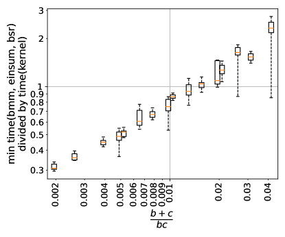
Figure 13: Speedup factor of kernel compared to $\min({\texttt{bmm}}{},{\texttt{einsum}}{},{\texttt{bsr}}{})$ in half-precision. For each implementation, we take the minimum time between the batch-size-first and the batch-size-last memory layout. We regroup the $(a,b,c,d)$ patterns by their value of $(b+c)/(bc)$, and use a boxplot to summarize the corresponding measurements. Experiments are carried in half-precision.

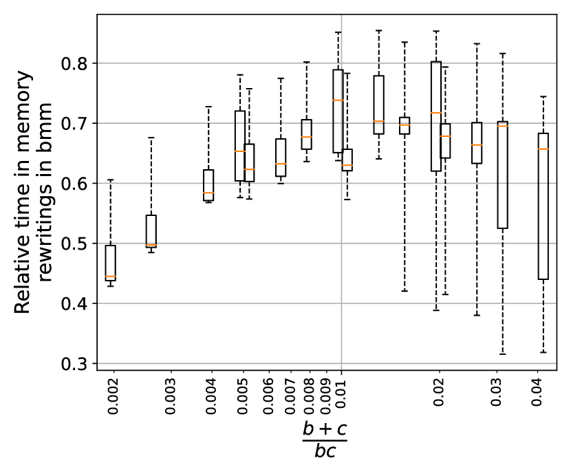
(a) Batch-size-first.

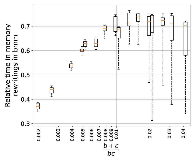
(b) Batch-size-last.

Figure 14: Estimated relative time spent on memory rewritings in bmm for the multiplication with $\mathbf{B}\in\Sigma^{{\boldsymbol{\pi}}}$, for several ${\boldsymbol{\pi}}=(a,b,c,d)$. We regroup patterns by their value of $(b+c)/(bc)$, and plot a boxplot to summarize the corresponding measurements. Experiments are carried in half-precision.

Figure 15: Speed-up factor of min time(kernel, bmm, bsr, einsum) compared to min time(dense, sparse) vs. the matrix size $M\times N$. Experiments are carried in half-precision.

Figure 16: Speed-up factor of time(bmm) compared to min time(einsum, bsr) vs. the matrix size $M\times N$. Experiments are carried in half-precision.

Appendix C Theoretical results

C.1 Details on perfect shuffle permutations

The goal is to prove Equation 1, which we recall here for convenience:

$$\mathbf{S}_{{\boldsymbol{\pi}}}=\underbrace{(\mathbf{I}_{a}\otimes\mathbf{P}_{b,d})}_{:=\mathbf{P}}\underbrace{(\mathbf{I}_{ad}\otimes\mathbf{1}_{b\times c})}_{=\mathbf{S}_{\tilde{{\boldsymbol{\pi}}}}}\underbrace{{(\mathbf{I}_{a}\otimes\mathbf{P}_{c,d})}^{\top}}_{:=\mathbf{Q}}=\mathbf{P}\mathbf{S}_{\tilde{{\boldsymbol{\pi}}}}\mathbf{Q},$$

where the matrix $\mathbf{P}_{p,q}$ is the so-called $(p,q)$ perfect shuffle permutation introduced below. To prove this formula, we will use the next lemma.

Lemma C.1.

For any positive integers $b,c,d$:

$${\mathbf{P}_{b,d}}^{\top}(\mathbf{1}_{b\times c}\otimes\mathbf{I}_{d})\mathbf{P}_{c,d}=\mathbf{I}_{d}\otimes\mathbf{1}_{b\times c},$$

where $\mathbf{P}_{p,q}$ denotes the $(p,q)$ perfect shuffle of $r:=pq$ [Van Loan, 2000], which is the permutation matrix of size $r\times r$ defined as:

$$\mathbf{P}_{p,q}:=\begin{pmatrix}{\mathbf{I}_{r}}[R_{0},:]\\ {\mathbf{I}_{r}}[R_{1},:]\\ \vdots\\ {\mathbf{I}_{r}}[R_{q-1},:]\end{pmatrix},$$ (3)

where $R_{i}:=\{i+qj\,|\,j\in\llbracket 0,p-1\rrbracket\}$ for $i\in\llbracket 0,q-1\rrbracket$.

Proof of Lemma C.1.

This is a direct consequence of a more general result claiming that the Kronecker product commutes up to some perfect shuffle permutation matrices [Van Loan, 2000, Section 1]. ∎

We now turn to the proof of Equation 1.

Proof of Equation 1.

By definition, $\mathbf{S}_{\boldsymbol{\pi}}=\mathbf{I}_{a}\otimes\mathbf{1}_{b\times c}\otimes\mathbf{I}_{d}$ when ${\boldsymbol{\pi}}=(a,b,c,d)$. By Lemma C.1,

$$\mathbf{S}_{\boldsymbol{\pi}}=\mathbf{I}_{a}\otimes\mathbf{1}_{b\times c}\otimes\mathbf{I}_{d}=\mathbf{I}_{a}\otimes\left(\mathbf{P}_{b,d}(\mathbf{I}_{d}\otimes\mathbf{1}_{b\times c}){\mathbf{P}_{c,d}}^{\top}\right).$$

By the equality $(\mathbf{A}\mathbf{B})\otimes(\mathbf{C}\mathbf{D})=(\mathbf{A}\otimes\mathbf{C})(\mathbf{B}\otimes\mathbf{D})$ for any matrices $\mathbf{A},\mathbf{B},\mathbf{C},\mathbf{D}$ of compatible sizes, we get the result:

$$\begin{split}\mathbf{S}_{\boldsymbol{\pi}}&=\mathbf{I}_{a}\otimes\left(\mathbf{P}_{b,d}(\mathbf{I}_{d}\otimes\mathbf{1}_{b\times c}){\mathbf{P}_{c,d}}^{\top}\right)\\ &=(\mathbf{I}_{a}\otimes\mathbf{P}_{b,d})\left(\mathbf{I}_{a}\otimes\left((\mathbf{I}_{d}\otimes\mathbf{1}_{b\times c}){\mathbf{P}_{c,d}}^{\top}\right)\right)\\ &=(\mathbf{I}_{a}\otimes\mathbf{P}_{b,d})(\mathbf{I}_{a}\otimes\mathbf{I}_{d}\otimes\mathbf{1}_{b\times c})(\mathbf{I}_{a}\otimes{\mathbf{P}_{c,d}}^{\top})\\ &=(\mathbf{I}_{a}\otimes\mathbf{P}_{b,d})(\mathbf{I}_{ad}\otimes\mathbf{1}_{b\times c})(\mathbf{I}_{a}\otimes{\mathbf{P}_{c,d}}^{\top}).\end{split}$$

∎

C.2 Existing variants of butterfly factorization

Table 8 summarizes how Definition 2.1 [Lin et al., 2021, Le, 2023] captures all the variants of butterfly factorizations that have been empirically tested for deep neural networks in the literature Dao et al. [2019, 2022a, 2022b], Vahid et al. [2020], Lin et al. [2021], Fu et al. [2023]. Note that the butterfly chain that we consider from Dao et al. [2022b] is the one used in their actual implementation rather than in their paper. A detailed explanation about this unification can be found in Chapter 6 of Le [2023], except for the case of block butterfly Dao et al. [2022a]. We now deal with the latter: we explain why block butterfly matrices are indeed covered by Definition 2.1.

Table 8: Definition 2.1 unifies the different factorizations tested for deep neural networks in the literature, as documented in Lin et al. [2021], Le [2023]. The fact that it also captures block butterfly matrices is new (Section C.2).

	Matrix size	Butterfly architecture
Dense	$M\times N$	$(1,M,N,1)$
Low-rank	$M\times N$	$(1,M,r,1),(1,r,N,1)$
Square dyadic [Dao et al., 2019, Vahid et al., 2020]	$N\times N$ with $N=2^{L}$	$(2^{\ell-1},2,2,2^{L-\ell})_{\ell=1}^{L}$
Kaleidoscope [Dao et al., 2022b]	$N\times N$ with $N=2^{L}$	Concatenate $(2^{\ell-1},2,2,2^{L-\ell})_{\ell=1}^{L}$ and $(2^{L-\ell},2,2,2^{\ell-1})_{\ell=1}^{L}$
Block butterfly [Dao et al., 2022a]	$N\times N$ with $N=2^{L}t$	$(2^{\ell-1},2t,2t,2^{L-\ell})_{\ell=1}^{L}$
Monarch [Dao et al., 2022b, Fu et al., 2023]	$M\times N$	$(1,M/p,\min(M,N)/p,p),(p,\min(M,N)/p,N/p,1)$
Deformable butterfly [Lin et al., 2021]	Introduced the general framework of Definition 2.1.

Block butterfly matrices are covered by Definition 2.1.

Block butterfly factors [Dao et al., 2022a] are a direct generalization of square dyadic butterfly factors [Dao et al., 2019]. Indeed, replacing each entry of a square dyadic butterfly factor by a block matrix of size $t\times t$ gives a block butterfly factor (and in particular, the square dyadic butterfly factors are particular cases of block butterfly factors with block size $1\times 1$.) The support constraints of block butterfly factors can be expressed by the following binary matrix [Dao et al., 2022a]:

$$\tilde{\mathbf{S}}_{\ell}:=\mathbf{I}_{2^{\ell-1}}\otimes\mathbf{1}_{2\times 2}\otimes\mathbf{I}_{2^{L-\ell}}\otimes\mathbf{1}_{t\times t},\qquad\qquad\ell=1,\ldots,L,$$ (4)

where we have an additional parameter $t$ in comparison to the tuples of butterfly factors (Definition 2.1) to control the block size.

We argue that using a chain of block butterfly factors (4) is equivalent to using a chain of butterfly factors in the sense of Definition 2.1. In order to prove that, we first introduce the set of matrices that can be factorized according to the two alternative definitions.

Definition C.2 (Set of block butterfly matrices).

Consider the chain of $L$ block butterfly factors of block size $t$, define $\mathcal{B}_{b}^{L,t}:=\{\prod_{\ell=1,\ldots,L}\mathbf{X}_{\ell}\mid\mathtt{supp}(\mathbf{X}_{\ell})\subseteq\mathtt{supp}(\tilde{\mathbf{S}}_{\ell})\}$ ($\tilde{\mathbf{S}}_{\ell}$ is defined as in (4)) the set of matrix admitting an exact factorization into block butterfly factors (shortened to block butterfly matrices).

Definition C.3 (Set of butterfly matrices associated to a butterfly chain $\Theta:=(\mathbf{t}_{\ell})_{\ell=1}^{L}$).

Consider a butterfly chain $\Theta:=(\mathbf{t}_{\ell})_{\ell=1}^{L}$, we define $\mathcal{B}^{\Theta}:=\{\prod_{\ell=1,\ldots,L}\mathbf{X}_{\ell}\mid\mathtt{supp}(\mathbf{X}_{\ell})\subseteq\mathtt{supp}(\mathbf{S}_{\mathbf{t}_{\ell}})\}$ the set of matrix admitting an exact factorization into butterfly factors (shortened to butterfly matrices).

The equivalence between block butterfly factors and butterfly chain is shown in the following lemma:

Lemma C.4.

Consider $\Theta:=(\mathbf{t}_{\ell})_{\ell=1}^{L}$ where $\mathbf{t}_{\ell}:=(2^{\ell-1},2t,2t,2^{L-\ell}),\ell=1,\ldots,L$, $\Theta$ is equivalent to the chain of $L$ block butterfly factors of block size $t$ in the sense that there exists two permutation matrices $(\mathbf{P},\mathbf{Q})$ of size $2^{L}t\times 2^{L}t$ such that:

$$\mathcal{B}^{L,t}_{b}=\mathbf{P}\mathcal{B}^{\Theta}\mathbf{Q}:=\{\mathbf{P}\mathbf{B}\mathbf{Q}\mid\mathbf{B}\in\mathcal{B}^{\Theta}\}.$$

In words, the two sets $\mathcal{B}^{L,t}_{b}$ and $\mathcal{B}^{\Theta}$ are expressively equivalent up to permutation of rows and columns.

Proof of Lemma C.4.

Consider the permutation matrices:

$$\mathbf{P}_{\ell}:=\mathbf{I}_{2^{\ell-1}}\otimes\mathbf{T}_{\ell}\qquad\mathbf{Q}_{\ell}:=\mathbf{I}_{2^{\ell}}\otimes\mathbf{T}_{\ell+1}^{\top},\quad\ell=1,\ldots,L,$$ (5)

where $\mathbf{T}_{\ell}$ (whose size is $2^{L-\ell+1}t\times 2^{L-\ell+1}t$) is the permutation matrix corresponding to the permutation:

$$\left(1,t+1,\ldots,(2^{L-\ell+1}-1)t+1,2,t+2,\ldots,(2^{L-\ell+1}-1)t+2,\ldots,t,2t,\ldots,2^{L-\ell+1}t\right).$$

The proof relies on the following claim:

$$\mathbf{P}_{\ell}\tilde{\mathbf{S}}_{\ell}\mathbf{Q}_{\ell}=\mathbf{S}_{\mathbf{t}_{\ell}},\qquad\forall\ell=1,\ldots,L,$$ (6)

which means that applying $\mathbf{P},\mathbf{Q}$ to the left and right of the $\ell$th block butterfly factors turn it into a $\mathbf{t}_{\ell}$-butterfly factors. Before proving (6), we explain how we can finish the proof of Lemma C.4 based on (6). Firstly, to prove the inclusion $\mathcal{B}_{b}^{L,t}\subseteq\mathbf{P}_{1}^{\top}\mathcal{B}^{\Theta}\mathbf{Q}_{\ell}^{\top}$, observe that:

$$\mathbf{Q}_{\ell-1}\mathbf{P}_{\ell} =(\mathbf{I}_{2^{\ell}}\otimes\mathbf{T}_{\ell}^{\top})(\mathbf{I}_{2^{\ell-1}}\otimes\mathbf{T}_{\ell})=\mathbf{I}_{2^{\ell-1}}\otimes(\mathbf{T}_{\ell}^{\top}\mathbf{T}_{\ell})=\mathbf{I}_{2^{\ell-1}}\otimes\mathbf{I}_{2^{L-\ell+1}t}=\mathbf{I}_{2^{L}t},$$ (7)

where we use the identity $(\mathbf{A}\otimes\mathbf{B})(\mathbf{C}\otimes\mathbf{D})=(\mathbf{A}\mathbf{C})\otimes(\mathbf{B}\mathbf{D})$ (applicable only when the matrix multiplication $\mathbf{A}\mathbf{C}$ and $\mathbf{B}\mathbf{D}$ is well-defined) and $\mathbf{P}\mathbf{P}^{\top}=\mathbf{I}$ for any permutation matrix. Thus, consider $(\tilde{\mathbf{X}}_{\ell})_{\ell=1,\ldots,L}$ a sequence of $L$ block butterfly factors of block size $t$, we have:

$$\tilde{\mathbf{X}}_{1}\tilde{\mathbf{X}}_{2}\ldots\tilde{\mathbf{X}}_{L} \overset{\eqref{eq:identityproduct}}{=}(\mathbf{P}_{1}^{\top}\mathbf{P}_{1})\tilde{\mathbf{X}}_{1}(\mathbf{Q}_{1}\mathbf{P}_{2})\tilde{\mathbf{X}}_{2}\ldots(\mathbf{Q}_{L-1}\mathbf{P}_{L})\tilde{\mathbf{X}}_{L}(\mathbf{Q}_{L}\mathbf{Q}_{L}^{\top})$$

$$\overset{\eqref{eq:transform}}{=}\mathbf{P}_{1}^{\top}\underbrace{(\mathbf{P}_{1}\tilde{\mathbf{X}}_{1}\mathbf{Q}_{1})}_{\mathbf{t}_{1}-\text{butterfly factor}}\underbrace{(\mathbf{P}_{2}\tilde{\mathbf{X}}_{2}\mathbf{Q}_{2})}_{\mathbf{t}_{2}-\text{butterfly factor}}\ldots\underbrace{(\mathbf{P}_{L}\tilde{\mathbf{X}}_{L}\mathbf{Q}_{L})}_{\mathbf{t}_{L}-\text{butterfly factor}}\mathbf{Q}_{L}^{\top}\in\mathbf{P}_{1}^{\top}\mathcal{B}^{\Theta}\mathbf{Q}_{L}^{\top}.$$

Therefore, $\mathcal{B}_{b}^{L,t}\subseteq\mathbf{P}_{1}^{\top}\mathcal{B}^{\Theta}\mathbf{Q}_{\ell}^{\top}$. Secondly, to see the other inclusion, from (6), we also have:

$$\mathbf{S}_{\ell}^{b}=\mathbf{P}_{\ell}^{\top}\mathbf{S}_{\mathbf{t}_{\ell}}\mathbf{Q}_{\ell}^{\top},\qquad\forall\ell=1,\ldots,L.$$ (8)

Similar to the proof of $\mathcal{B}_{b}^{L,t}\subseteq\mathbf{P}_{1}^{\top}\mathcal{B}^{\Theta}\mathbf{Q}_{L}^{\top}$, we can consider $(\mathbf{X}_{\ell})_{\ell=1,\ldots,L}$ where $\mathbf{X}_{\ell}$ is a $\mathbf{t}_{\ell}$-butterfly factor. We have:

$$\mathbf{P}_{1}^{\top}\mathbf{X}_{1}\mathbf{X}_{2}\ldots\mathbf{X}_{L}\mathbf{Q}_{\ell}^{\top} \overset{\eqref{eq:identityproduct}}{=}\mathbf{P}_{1}^{\top}\mathbf{X}_{1}(\mathbf{P}_{2}\mathbf{Q}_{1})^{\top}\mathbf{X}_{2}\ldots\mathbf{X}_{L-1}(\mathbf{P}_{L}\mathbf{Q}_{L-1})^{\top}\mathbf{X}_{L}^{b}\mathbf{Q}_{L}^{\top}$$

$$\overset{\eqref{eq:transform2}}{=}\underbrace{(\mathbf{P}_{1}^{\top}\mathbf{X}_{1}\mathbf{Q}_{1}^{\top})}_{1\text{st block butterfly factor}}\ldots\underbrace{(\mathbf{P}_{L}^{\top}\mathbf{X}_{L}\mathbf{Q}_{L}^{\top})}_{L\text{th block butterfly factor}}\in\mathcal{B}_{b}^{L,t}.$$

Thus, $\mathbf{P}_{1}^{\top}\mathcal{B}^{\Theta}\mathbf{Q}_{\ell}^{\top}\subseteq\mathcal{B}_{b}^{L,t}$. We can conclude that $\mathbf{P}_{1}^{\top}\mathcal{B}^{\Theta}\mathbf{Q}_{\ell}^{\top}=\mathcal{B}_{b}^{L,t}$ and the pair of permutation matrices $(\mathbf{P}_{1}^{\top},\mathbf{Q}_{L}^{\top})$ satisfies Lemma C.4.

Finally, it remains to prove (6). Using the identity: $(\mathbf{A}_{1}\otimes\ldots\otimes\mathbf{A}_{n})(\mathbf{B}_{1}\otimes\ldots\otimes\mathbf{B}_{n})(\mathbf{C}_{1}\otimes\ldots\otimes\mathbf{C}_{n})=(\mathbf{A}_{1}\mathbf{B}_{1}\mathbf{C}_{1})\otimes\ldots\otimes(\mathbf{A}_{n}\mathbf{B}_{n}\mathbf{C}_{n})$ (when $\mathbf{A}_{\ell}\mathbf{B}_{\ell}\mathbf{C}_{\ell},\ell=1,\ldots,n$ makes sense), we have:

$$\mathbf{P}_{\ell}\mathbf{S}_{\ell}^{b}\mathbf{Q}_{\ell} =(\mathbf{I}_{2^{\ell-1}}\otimes\mathbf{T}_{\ell})(\mathbf{I}_{2^{\ell-1}}\otimes\mathbf{1}_{2\times 2}\otimes\mathbf{I}_{2^{L-\ell}}\otimes\mathbf{1}_{t\times t})(\mathbf{I}_{2^{\ell}}\otimes\mathbf{T}_{\ell+1}^{\top})$$

$$=\mathbf{I}_{2^{\ell-1}}\otimes[\mathbf{T}_{\ell}(\mathbf{1}_{2\times 2}\otimes\mathbf{I}_{2^{L-\ell}}\otimes\mathbf{1}_{t\times t})(\mathbf{I}_{2}\otimes\mathbf{T}_{\ell+1}^{\top})],\forall\ell=1,\ldots,L.$$

Thus, it is sufficient to prove that:

$$\mathbf{T}_{\ell}(\mathbf{1}_{2\times 2}\otimes\mathbf{I}_{2^{L-\ell}}\otimes\mathbf{1}_{t\times t})(\mathbf{I}_{2}\otimes\mathbf{T}_{\ell+1}^{\top})=\mathbf{1}_{2t\times 2t}\otimes\mathbf{I}_{2^{L-\ell}},\forall\ell=1,\ldots,L.$$

To show the equation above, we will use an ad-hoc argument. Note that the binary matrix $\mathbf{1}_{2\times 2}\otimes\mathbf{I}_{2^{L-\ell}}\otimes\mathbf{1}_{t\times t}$ has exactly $2^{L-\ell}$ different columns (resp. rows). If we partition them into $2^{L-\ell}$ groups $\{1,\ldots,2^{L-\ell}\}$ and label each of them by the partition they belong to, then the columns and rows will have the form:

$$(\underbrace{1,\ldots,1}_{t\text{ times}},\underbrace{2,\ldots,2}_{t\text{ times}},\ldots,\underbrace{2^{L-\ell},\ldots,2^{L-\ell}}_{t\text{ times}},\underbrace{1,\ldots,1}_{t\text{ times}},\underbrace{2,\ldots,2}_{t\text{ times}},\ldots,\underbrace{2^{L-\ell},\ldots,2^{L-\ell}}_{t\text{ times}}).$$

This procedure of labeling can be visualized as in Figure 18 for a simple case where $L-\ell=1$ and $t=3$.

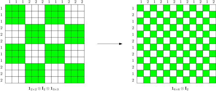
Figure 18: Illustration for the proof of (6). Green and white squares represent the $1$s and $0$s of the binary matrices respectively.

To turn $\mathbf{1}_{2\times 2}\otimes\mathbf{I}_{2^{L-\ell}}\otimes\mathbf{1}_{t\times t}$ into $\mathbf{1}_{2t\times 2t}\otimes\mathbf{I}_{2^{L-\ell}}$, the permutation matrices on the left and right (in this case, $\mathbf{T}_{\ell}$ and $\mathbf{I}_{2}\otimes\mathbf{T}_{\ell+1}^{\top}$) need to permute the columns and rows such that the label becomes:

$$(\underbrace{1,2,\ldots,2^{L-\ell}}_{1\text{st}},\underbrace{1,2,\ldots,2^{L-\ell}}_{2\text{nd}},\ldots,\underbrace{1,2,\ldots,2^{L-\ell}}_{2t\text{th}}).$$

It can be seen directly that $\mathbf{T}_{\ell}$ permutes the label of the rows correctly. For $\mathbf{I}_{2}\otimes\mathbf{T}_{\ell+1}^{\top}$, this permutation matrix permutes the columns in the first half and the second half separately (due to the Kronecker product with $\mathbf{I}_{2}$) and each half is permuted by the permutation described in (5). Thanks to this interpretation, it can be seen that $\mathbf{I}_{2}\otimes\mathbf{T}_{\ell+1}^{\top}$ also permutes the label of the columns correctly as well. This concludes the proof. ∎

Appendix D Implementations

D.1 Details on baseline GPU implementations

To keep it short, we only give the code in the case of the batch-size-first memory layout (except for dense and sparse where the codes are small). The case of batch-size-last can simply be obtained by inverting the first and last positions in all tensor reshapings.

einsum implementation. This implementation uses tensor contractions with the high-performance einops library. The $abcd$ nonzero entries of the butterfly factor $\mathbf{B}$ (Figure 2) are stored in a PyTorch 4D-tensor B_einsum of shape $(a,b,c,d)$. The implementation uses Einstein notations.

⬇

1def butterfly_einsum(X_bsf, B_einsum):

2 X_perm = einops.rearrange(X_bsf, "... (a c d) -> ... a c d", a=a, c=c, d=d)

3 Y_perm = einops.einsum(X_perm, B_einsum, "... a c d, a b c d -> ... a b d")

4 Y_bsf = einops.rearrange(Y_perm, "... a b d-> ... (a b d)")

5 return Y_bsf

The second line of this code does at the same time all the matrix multiplications ${\mathbf{Y}}[:,\texttt{row}]\leftarrow{\mathbf{X}}[:,\texttt{col}]{{\mathbf{B}}^{\top}}[\texttt{col},\texttt{row}]$ for all the pairs $(\texttt{row},\texttt{col})$ in Algorithm 1.

bsr implementation. This is an implementation of Algorithm 2 using the high-performance Block compressed Sparse Row (BSR) PyTorch library. The matrix $\tilde{\mathbf{B}}$ is stored as a tensor B_bsr stored in the BSR format.

⬇

1def butterfly_bsr(X_bsf, B_bsr):

2 batch_size = X_bsf.shape[0]

3 X_perm = (

4 X_bsf.view(batch_size, a, c, d)

5 .transpose(-1, -2)

6 .reshape(batch_size, a * c * d)

7 )

8 Y_perm = torch.nn.functional.linear(

9 X_perm, B_bsr

10 )

11 Y_bsf = (

12 Y_perm.view(batch_size, a, d, b)

13 .transpose(-1, -2)

14 .reshape(batch_size, a * b * d)

15 )

16 return Y_bsf

bmm implementation. This is an implementation of Algorithm 2 using the high-performance Block compressed Sparse Row (BSR) PyTorch library. The matrix $\tilde{\mathbf{B}}$ is stored as a tensor B_bsr stored in the BSR format. This implementation using torch.bmm, which is based on high-performance batched matrix multiplication NVIDIA routines. The non-zero entries of $\tilde{\mathbf{B}}$ are stored in a four-dimensional PyTorch tensor B_bmm of shape $(a*d,b,c)$.

⬇

1def butterfly_bmm(X_bsf, B_bmm):

2 batch_size = X_bsf.shape[0]

3 X_perm = (

4 X_bsf.view(batch_size, a, c, d)

5 .transpose(-1, -2)

6 .reshape(batch_size, a * d, c).

7 contiguous().

8 transpose(0, 1)

9 )

10 Y_perm = torch.empty(batch_size, a * d, b, device=x.device, dtype=x.dtype).transpose(0, 1)

11 Y_perm = torch.bmm(X_perm, B_bmm.transpose(-1, -2))

12 Y_bsf = (

13 Y_perm.transpose(0, 1)

14 .reshape(batch_size, a, d, b)

15 .transpose(-1, -2)

16 .reshape(batch_size, a * b * d)

17 )

18 return

dense implementation. This ignores the sparsity of the butterfly factor $\mathbf{B}$, that is stored as a dense matrix in a 2d-tensor B_dense.

batch-size-first: torch.nn.functional.linear(${\texttt{X\_bsf}},{\texttt{B\_dense}}$)

batch-size-last: torch.matmul(${\texttt{B\_dense}},{\texttt{X\_bsl}}$)

The implementation in batch-size-first is the default PyTorch implementation of a forward pass of a linear layer. For batch-size-last, we had to choose an implementation since Pytorch uses batch-size-first by default. We made our choice based on a small benchmark of different alternatives.

sparse implementation. This exploits the sparsity of the butterfly factor $\mathbf{B}$ but not its structure (recall that the support are not arbitrary, they are structured since they must be expressed as Kronecker products, see Definition 2.1).

batch-size-first: torch.nn.functional.linear(${\texttt{X\_bsf}},{\texttt{B\_csr}}$)

batch-size-last: torch.matmul(${\texttt{B\_csr}},{\texttt{X\_bsl}}$)

D.2 Details on the kernel implementation

Classical optimizations that we build upon. The proposed implementation use vectorization as soon as an operation can be vectorized. Concretely, the float4 and half2 vector types are used to mutualize read/write operations [NVIDIA, 2023b, a, 2024, Boehm, 2022]. An epilogue [NVIDIA, 2023a] is also implemented to avoid writing in global memory in a disorganized way. Indeed, after having accumulated the output in registers, each thread has specific rows and columns of the output to write to global memory, and may finish its computation before the others. To avoid that, the epilogue starts to write in the shared memory, in a disorganized way, and then organize the writing from shared to global memory. Another implemented optimization is double buffering NVIDIA [2023b, a], Boehm [2022], Li et al. [2019]: a thread block is always both computing the output of a tile, and loading the next tile from global to shared memory. This allows us to hide some latency that arises when loading from the global memory.

Note that as with any CUDA kernel, the constants (such as the number of threads) need to be tailored to each specific case of use —here, each butterfly sparsity pattern ${\boldsymbol{\pi}}=(a,b,c,d)$— and to each GPU.

References

- Boehm (2022) Simon Boehm. How to optimize a CUDA matmul kernel for cuBLAS-like performance: A worklog, 2022. https://siboehm.com/articles/22/CUDA-MMM [Accessed: April 2024].
- Dao et al. (2019) Tri Dao, Albert Gu, Matthew Eichhorn, Atri Rudra, and Christopher Ré. Learning fast algorithms for linear transforms using butterfly factorizations. In ICML, 2019.
- Dao et al. (2022a) Tri Dao, Beidi Chen, Kaizhao Liang, Jiaming Yang, Zhao Song, Atri Rudra, and Christopher Re. Pixelated butterfly: Simple and efficient sparse training for neural network models. In ICLR, 2022a.
- Dao et al. (2022b) Tri Dao, Beidi Chen, Nimit S Sohoni, Arjun Desai, Michael Poli, Jessica Grogan, Alexander Liu, Aniruddh Rao, Atri Rudra, and Christopher Ré. Monarch: Expressive structured matrices for efficient and accurate training. In ICML, 2022b.
- Dao et al. (2022c) Tri Dao, Dan Fu, Stefano Ermon, Atri Rudra, and Christopher Ré. Flashattention: Fast and memory-efficient exact attention with io-awareness. Advances in Neural Information Processing Systems, 35:16344–16359, 2022c.
- Dosovitskiy et al. (2020) Alexey Dosovitskiy, Lucas Beyer, Alexander Kolesnikov, Dirk Weissenborn, Xiaohua Zhai, Thomas Unterthiner, Mostafa Dehghani, Matthias Minderer, Georg Heigold, Sylvain Gelly, et al. An image is worth 16x16 words: Transformers for image recognition at scale. In ICLR, 2020.
- Fu et al. (2023) Daniel Y Fu, Simran Arora, Jessica Grogan, Isys Johnson, Sabri Eyuboglu, Armin W Thomas, Benjamin Spector, Michael Poli, Atri Rudra, and Christopher Ré. Monarch mixer: A simple sub-quadratic GEMM-based architecture. In NeurIPS, 2023.
- Gribonval et al. (2023) Rémi Gribonval, Theo Mary, and Elisa Riccietti. Optimal quantization of rank-one matrices in floating-point arithmetic—with applications to butterfly factorizations. preprint, 2023. URL https://inria.hal.science/hal-04125381.
- HPCwire (2019) HPCwire. AWS Upgrades its GPU-Backed AI Inference Platform. https://www.hpcwire.com/2019/03/19/aws-upgrades-its-gpu-backed-ai-inference-platform/, March 2019. Accessed: [April 2024].
- Jeff Barr (2019) Jeff Barr. Amazon EC2 Update – Inf1 Instances with AWS Inferentia Chips for High Performance Cost-Effective Inferencing. aws.amazon.com/blogs/aws/amazon-ec2-update-inf1-instances-with-aws-inferentia-chips-for-high-performance-cost-effective-inferencing, 2019. Accessed: [April 2024].
- Le (2023) Quoc-Tung Le. Algorithmic and theoretical aspects of sparse deep neural networks. PhD thesis, 2023. URL https://inria.hal.science/tel-04329531.
- Le et al. (2022) Quoc-Tung Le, Léon Zheng, Elisa Riccietti, and Rémi Gribonval. Fast learning of fast transforms, with guarantees. In ICASSP, 2022.
- Li et al. (2019) Xiuhong Li, Yun Liang, Shengen Yan, Liancheng Jia, and Yinghan Li. A coordinated tiling and batching framework for efficient GEMM on GPUs. In Proceedings of the 24th Symposium on Principles and Practice of Parallel Programming, 2019.
- Lin et al. (2021) Rui Lin, Jie Ran, King Hung Chiu, Graziano Chesi, and Ngai Wong. Deformable butterfly: A highly structured and sparse linear transform. In NeurIPS, 2021.
- NVIDIA (2023a) NVIDIA. Efficient GEMM in CUDA: documentation, 2023a. https://github.com/NVIDIA/cutlass/blob/main/media/docs/efficient_gemm.md [Accessed: April 2024].
- NVIDIA (2023b) NVIDIA. Matrix multiplication background user’s guide, 2023b. https://docs.nvidia.com/deeplearning/performance/dl-performance-matrix-multiplication/index.html [Accessed: April 2024].
- NVIDIA (2024) NVIDIA. CUDA C++ programming guide, 2024. https://docs.nvidia.com/cuda/cuda-c-programming-guide/index.html [Accessed: April 2024].
- Quemener and Corvellec (2013) E. Quemener and M. Corvellec. SIDUS—the Solution for Extreme Deduplication of an Operating System. Linux Journal, 2013.
- Rogozhnikov (2021) Alex Rogozhnikov. Einops: Clear and reliable tensor manipulations with einstein-like notation. In ICLR, 2021.
- Vahid et al. (2020) Keivan Alizadeh Vahid, Anish Prabhu, Ali Farhadi, and Mohammad Rastegari. Butterfly transform: An efficient FFT based neural architecture design. In CVPR, 2020.
- Van Loan (2000) Charles F Van Loan. The ubiquitous kronecker product. Journal of computational and applied mathematics, 123(1-2):85–100, 2000.
- Wang (2024a) Phil Wang. Scaled dot-product attention implementation, 2024a. https://docs.nvidia.com/deeplearning/performance/dl-performance-matrix-multiplication/index.html [Accessed: April 2024].
- Wang (2024b) Phil Wang. Simple ViT implementation, 2024b. https://github.com/lucidrains/vit-pytorch/blob/main/vit_pytorch/simple_vit.py [Accessed: April 2024].
- Zhai et al. (2022) Xiaohua Zhai, Alexander Kolesnikov, Neil Houlsby, and Lucas Beyer. Scaling vision transformers. In CVPR, 2022.
- Zheng et al. (2023) Léon Zheng, Elisa Riccietti, and Rémi Gribonval. Efficient identification of butterfly sparse matrix factorizations. SIAM Journal on Mathematics of Data Science, 5(1):22–49, 2023.