Lower Bound on the Greedy Approximation Ratio
for Adaptive Submodular Cover

Abstract

We show that the greedy algorithm for adaptive-submodular cover has approximation ratio at least $1.3\times(1+\ln Q)$. Moreover, the instance demonstrating this gap has $Q=1$. So, it invalidates a prior result in the paper “Adaptive Submodularity: A New Approach to Active Learning and Stochastic Optimization” by Golovin-Krause, that claimed a $(1+\ln Q)^{2}$-approximation ratio for the same algorithm.

1 Introduction

Adaptive-submodularity is a widely used framework in stochastic optimization and machine learning [GK11, GK17, EKM21, ACN22]. Here, an algorithm makes sequential decisions while (partially) observing uncertainty. We study a basic problem in this context: covering an adaptive-submodular function at the minimum expected cost. We show that the natural greedy algorithm for this problem has approximation ratio at least $1.3\times(1+\ln Q)$, where $Q$ is the maximal function value. This is in contrast to special cases such as deterministic submodular cover or (independent) stochastic submodular cover, where the greedy algorithm achieves a tight $(1+\ln Q)$ approximation ratio.

1.1 Problem Definition

The following definitions and problem description are borrowed from [ACN22].

Random items.

Let $E$ be a finite set of $n$ items. Each item $e\in E$ corresponds to a random variable $\Phi_{e}\in\Omega$, where $\Omega$ is the outcome space (for a single item). We use $\Phi=\langle\Phi_{e}:e\in E\rangle$ to denote the vector of all random variables (r.v.s). The r.v.s may be arbitrarily correlated across items. We use upper-case letters to represent r.v.s and the corresponding lower-case letters to represent realizations of the r.v.s. Thus, for any item $e$, $\phi_{e}\in\Omega$ is the realization of $\Phi_{e}$; and $\phi=\langle\phi_{e}:e\in E\rangle$ denotes the realization of $\Phi$. Equivalently, we can represent the realization $\phi$ as a subset $\{(e,\phi_{e}):e\in E\}\subseteq E\times\Omega$ of item-outcome pairs.

A partial realization $\psi\subseteq E\times\Omega$ refers to the realizations of any subset of items; $\mathsf{dom}(\psi)\subseteq E$ denotes the items whose realizations are represented in $\psi$, and $\psi_{e}$ denotes the realization of any item $e\in\mathsf{dom}(\psi)$. Note that a partial realization contains at most one pair of the form $(e,*)$ for any item $e\in E$. The (full) realization $\phi$ corresponds to a partial realization with $\mathsf{dom}(\phi)=E$. For two partial realizations $\psi,\psi^{\prime}\subseteq E\times\Omega$, we say that $\psi$ is a subrealization of $\psi{{}^{\prime}}$ (denoted $\psi\preccurlyeq\psi{{}^{\prime}}$) if $\psi\subseteq\psi^{\prime}$; in other words, $\mathsf{dom}(\psi)\subseteq\mathsf{dom}(\psi^{\prime})$ and $\psi_{e}=\psi^{\prime}_{e}$ for all $e\in\mathsf{dom}(\psi)$. Two partial realizations $\psi,\psi^{\prime}\subseteq E\times\Omega$ are said to be disjoint if there is no full realization $\phi$ with $\psi\preccurlyeq\phi$ and $\psi^{\prime}\preccurlyeq\phi$; in other words, there is some item $e\in\mathsf{dom}(\psi)\cap\mathsf{dom}(\psi^{\prime})$ such that the realization of $\Phi_{e}$ is different under $\psi$ and $\psi^{\prime}$.

We assume that there is a prior probability distribution $p(\phi)=\Pr[\Phi=\phi]$ over realizations $\phi$. Moreover, for any partial realization $\psi$, we assume that we can compute the posterior distribution $p(\phi|\psi)=\Pr(\Phi=\phi|\psi\preccurlyeq\Phi).$

Utility function.

In addition to the random items (described above), there is a utility function $f:2^{E\times\Omega}\to\mathbb{R}_{\geq 0}$ that assigns a value to any partial realization. We will assume that this function is monotone, i.e., having more realizations can not reduce the value. Formally,

Definition 1.1 (Monotonicity).

A function $f:2^{E\times\Omega}\to\mathbb{R}_{\geq 0}$ is monotone if

$$f(\psi)\leq f(\psi^{\prime})\quad\mbox{ for all partial realizations }\psi\preccurlyeq\psi{{}^{\prime}}.$$

We also assume that the function $f$ can always achieve its maximal value, i.e.,

Definition 1.2 (Coverable).

Let $Q$ be the maximal value of function $f$. Then, function $f$ is said to be coverable if this value $Q$ can be achieved under every (full) realization, i.e.,

$$f(\phi)=Q\mbox{ for all realizations $\phi$ of }\Phi.$$

Furthermore, we will assume that the function $f$ along with the probability distribution $p(\cdot)$ satisfies a submodularity-like property. Before formalizing this, we need the following definition.

Definition 1.3 (Marginal benefit).

The conditional expected marginal benefit of an item $e\in E$ conditioned on observing the partial realization $\psi$ is:

$$\Delta(e|\psi):=\mathbb{E}\left[f(\psi\cup(e,\Phi_{e}))-f(\psi)\,|\,\psi\preccurlyeq\Phi\right]\,\,=\,\,\sum_{\omega\in\Omega}\Pr[\Phi_{e}=\omega|\psi\preccurlyeq\Phi]\cdot\left(f(\psi\cup(e,\omega))-f(\psi)\right).$$

We will assume that function $f$ and distribution $p(\cdot)$ jointly satisfy the adaptive-submodularity property, defined as follows.

Definition 1.4 (Adaptive submodularity).

A function $f:2^{E\times\Omega}\to\mathbb{R}_{\geq 0}$ is adaptive submodular w.r.t. distribution $p(\phi)$ if for all partial realizations $\psi\preccurlyeq\psi^{{}^{\prime}}$, and all items $e\in E\setminus\mathsf{dom}(\psi^{{}^{\prime}})$, we have

$$\Delta(e|\psi)\geq\Delta(e|\psi^{{}^{\prime}}).$$

In other words, this property ensures that the marginal benefit of an item never increases as we condition on more realizations. Given any function $f$ satisfying Definitions 1.1, 1.2 and 1.4, we can pre-process $f$ by subtracting $f(\emptyset)$, to get an equivalent function (that maintains these properties), and has a smaller $Q$ value. So, we may assume that $f(\emptyset)=0$.

Min-cost adaptive-submodular cover (${\sf ASC}$).

In this problem, each item $e\in E$ has a positive cost $c_{e}$. The goal is to select items (and observe their realizations) sequentially until the observed realizations have function value $Q$. The objective is to minimize the expected cost of selected items.

Due to the stochastic nature of the problem, the solution concept here is much more complex than in the deterministic setting (where we just select a static subset). In particular, a solution corresponds to a “policy” that maps observed realizations to the next selection decision. The observed realization at any point corresponds to a partial realization (namely, the realizations of the items selected so far). Formally, a policy is a mapping $\pi:2^{E\times\Omega}\to E$, which specifies the next item $\pi(\psi)$ to select when the observed realizations are $\psi$. The policy $\pi$ terminates at the first point when $f(\psi)=Q$, where $\psi\subseteq E\times\Omega$ denotes the observed realizations so far. For any policy $\pi$ and full realization $\phi$, let $C(\pi,\phi)$ denote the total cost of items selected by policy $\pi$ under realization $\phi$. Then, the expected cost of policy $\pi$ is:

$$c_{exp}(\pi)\,\,=\,\,\mathbb{E}_{\Phi}\left[C(\pi,\Phi)\right]\,\,=\,\,\sum_{\phi}p(\phi)\cdot C(\pi,\phi).$$

At any point in policy $\pi$, we refer to the cumulative cost incurred so far as the time. If $J_{1},J_{2},\cdots J_{k}$ denotes the (random) sequence of items selected by $\pi$ then for each $i\in\{1,2,\cdots k\}$, we view item $J_{i}$ as being selected during the time interval $[\sum_{h=1}^{i-1}c(J_{h})\,,\,\sum_{h=1}^{i}c(J_{h}))$ and the realization of $J_{i}$ is only observed at time $\sum_{h=1}^{i}c(J_{h})$. For any time $t\geq 0$, we use $\Psi(\pi,t)\subseteq E\times\Omega$ to denote the (random) realizations that have been observed by time $t$ in policy $\pi$. We note that $\Psi(\pi,t)$ only contains the realizations of items that have been completely selected by time $t$. Note that the policy terminates at the earliest time $t$ where $f(\Psi(\pi,t))=Q$.

Remark:

Our definition of the utility function $f$ is slightly more restrictive than the original definition [GK11, GK17]. In particular, the utility function in [GK11] is of the form $g:2^{E}\times\Omega^{E}\rightarrow\mathbb{R}_{\geq 0}$, where the function value $g(\mathsf{dom}(\psi),\Phi)$ for any partial realization $\psi$ is still random and can depend on the outcomes of unobserved items, i.e., those in $E\setminus\mathsf{dom}(\psi)$. We note that the ${\sf ASC}$ formulation satisfies “strong adaptive monotonicity”, “strong adaptive submodularity” and the “self certifying” condition defined in [GK17]

1.2 Adaptive Greedy Policy

Algorithm 1 describes a natural greedy policy for min-cost adaptive-submodular cover, which has also been studied in prior works [GK17, EKM21, HKP21, ACN22].

Algorithm 1 Adaptive Greedy Policy $\pi$.

1:selected items $A\leftarrow\emptyset$, observed realizations $\psi\leftarrow\emptyset$

2:while $f(\psi)<Q$ do

3:     $e^{*}=\operatorname*{arg\,max}_{e\in E\setminus A}\frac{\Delta(e|\psi)}{c_{e}}$

4:     add $e^{*}$ to the selected items, i.e., $A\leftarrow A\cup\{e^{*}\}$

5:     select $e^{*}$ and observe $\Phi_{e^{*}}$

6:     update $\psi\leftarrow\psi\cup\{(e^{*},\Phi_{e^{*}})\}$

1.3 Prior Results on the Greedy Policy

The above greedy policy is known to have strong performance guarantees for adaptive submodular cover and even better performance in several special cases. We now discuss these results in detail. Here, we assume that the function $f$ is integer valued (to keep notation simple).

In the deterministic setting of submodular cover (which is a classic problem in combinatorial optimization), [Wol82] proved that this greedy algorithm achieves a $1+\ln Q$ approximation. Previously, such an approximation ratio was known in the special case of set cover [Chv79], where $Q$ equals the number of elements to cover. Furthermore, assuming $P\neq NP$, there one cannot achieve any $(1-o(1))\ln Q$ approximation ratio for set cover [DS14].

The independent special case of adaptive-submodular cover (called stochastic submodular cover) has itself been studied extensively. Here, the random variables $\Phi_{e}$ are independent across items $e\in E$. The greedy policy was shown to achieve an $O(\ln Q)$ approximation ratio in [INvdZ16], and recently [HKP21] proved that the greedy policy has a sharp $(1+\ln Q)$ approximation guarantee.

Moving beyond the independent setting, [GK11] introduced adaptive-submodular cover (in a slightly more general form than ${\sf ASC}$) and claimed that the greedy policy has a $(1+\ln Q)$ approximation ratio. This proof had a flaw, which was pointed out by [NS17]. Subsequently, [GK17] posted an updated result proving a $(1+\ln Q)^{2}$ approximation ratio. Then, [EKM21] proved a bound of $(1+\ln(nQc_{max}))$ for the greedy policy; note that this bound depends additionally on the number of items $n$ and their maximum cost $c_{max}$. Recently, [ACN22] proved that the greedy policy is a $4\cdot(1+\ln Q)$ approximation algorithm.

1.4 Our Result

In light of the above results, it was natural to expect that the greedy policy for ${\sf ASC}$ should also have a $(1+\ln Q)$ approximation ratio. This would match the bounds known in the deterministic [Wol82] and independent [HKP21] special cases. It would also match the in-approximability threshold known in the (very) special case of set cover [DS14]. However, we show that the greedy policy for ${\sf ASC}$ cannot achieve a $(1+\ln Q)$ approximation ratio. Specifically,

Theorem 1.1.

There are instances of adaptive submodular cover with integer-valued function $f$ and $Q=1$ where the greedy policy has expected cost at least $\rho>1$ times the optimum.

In the next section, we provide a small instance (with $n=4$ items) and prove that the constant $\rho\geq 1.15$. However, this constant factor can be increased using more complex instances and computer-assisted calculations: we could obtain $\rho\geq 1.3$.

Our result also disproves Theorem 40 in [GK17] that states a $(1+\ln Q)^{2}$ approximation ratio for the greedy policy for ${\sf ASC}$: this is because our “hard” instance has $Q=1$. So, if the result in [GK17] were correct then the greedy policy should be optimal on our instance.

2 Hard Instance for Greedy

We now prove Theorem 1.1.

Our instance consists of $n=4$ items $E=\{a,b,c,d\}$ with outcome space $\Omega=\{0,1\}$. The item realizations are determined by a set of $4$ independent Bernoulli r.v.s $X_{1},X_{2},X_{3},X_{4}\sim\mathsf{Ber}(1-p)$ where the probability $p$ will be set later. We have

$$\Phi_{a}=\begin{cases}1\text{ if }X_{1}+X_{2}\geq 1\\ 0\text{ otherwise}\end{cases},\quad\Phi_{b}=\begin{cases}1\text{ if }X_{3}+X_{4}\geq 1\\ 0\text{ otherwise}\end{cases},\quad\Phi_{c}=\begin{cases}1\text{ if }X_{1}+X_{3}\geq 1\\ 0\text{ otherwise}\end{cases}.$$

The element $d$ always realizes to $1$, i.e., $\Phi_{d}=1$ with probability $1$. See Figure 1.

We set the costs of items $\{a,b,c\}$ to be $1$ each and item $d$ has cost $\frac{1}{1-p}$.

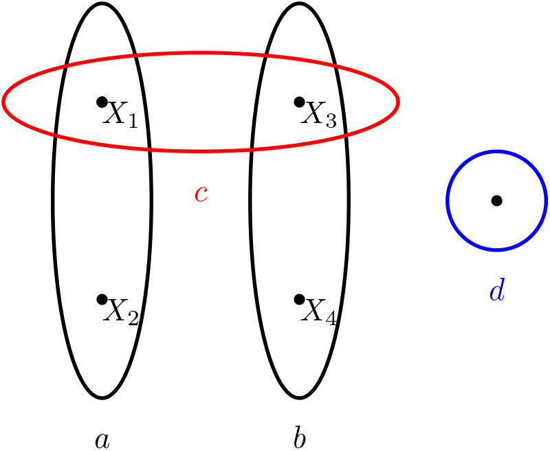
Figure 1: The r.v.s $\{X_{i}\}_{i=1}^{4}$ and items $\{a,b,c,d\}$.

The utility function $f:2^{E\times\Omega}\rightarrow\mathbb{Z}_{+}$ corresponds to observing some “$1$ outcome”. That is, if we let $E^{*}=\{(e,1):e\in E\}$ denote all the $1$-outcome-item pairs then

$$f(\psi)=\min\{|\psi\cap E^{*}|,1\},\qquad\forall\psi\subseteq E\times\Omega.$$

Note that $f$ is a coverage function: so it is monotone submodular and has maximal value $Q=1$.

We now show that this instance satisfies all the assumptions for ${\sf ASC}$: Definitions 1.1, 1.2 and Definition 1.4. Clearly, function $f$ is monotone: so Definition 1.1 holds. Moreover, every full realization $\phi$ has $\phi_{d}=1$: so $f(\phi)=1=Q$, which means Definition 1.2 holds.

Adaptive submodularity.

We now show that Definition 1.4 holds. Suppose $\psi$ and $\psi^{\prime}$ are partial realizations with $\psi\preccurlyeq\psi^{\prime}$ and item $e\in E\setminus\mathsf{dom}(\psi^{\prime})$. Now let us examine multiple cases.

1. $f(\psi^{\prime})=1$ : in this case, $\Delta(e|\psi^{\prime})=0$ as $1$ is the maximum value of $f$. So, $\Delta(e|\psi)\geq\Delta(e|\psi^{\prime})$.

2. $d\in dom(\psi^{\prime})\cup e$ : if $d\in\mathsf{dom}(\psi^{\prime})$ then $f(\psi^{\prime})=1$ and we fall into case 1 above. If $e=d$ then $f(\psi\cup\{(d,\Phi_{d})\})=1$, which combined with $f(\psi)\leq f(\psi^{\prime})$ implies $\Delta(e|\psi)\geq\Delta(e|\psi^{\prime})$.

3. All remaining cases are summarized in Table 1 or follow using the symmetry between items $a$ and $b$. In each of these cases, we can directly calculate $\Delta(e|\psi)$ and $\Delta(e|\psi^{\prime})$. E.g., consider the case $\psi=\emptyset$, $\psi^{\prime}=(a,0)$ and $e=c$: we have $\Delta(e|\psi)=\Pr[X_{1}=1\vee X_{3}=1]=1-p^{2}$ and $\Delta(e|\psi^{\prime})=\Pr[X_{1}=1\vee X_{3}=1|X_{1}=X_{2}=0]=1-p$.

$\psi$	$\psi^{\prime}$	item $e$	$\Delta(e|\psi)$	$\Delta(e|\psi^{\prime})$
$\emptyset$	$(a,0)$	$b$	$1-p^{2}$	$1-p^{2}$
$\emptyset$	$(a,0)$	$c$	$1-p^{2}$	$1-p$
$\emptyset$	$(c,0)$	$a$	$1-p^{2}$	$1-p$
$\emptyset$	$(a,0)\ (b,0)$	$c$	$1-p^{2}$	$0$
$\emptyset$	$(a,0)\ (c,0)$	$b$	$1-p^{2}$	$1-p$
$(a,0)$	$(a,0)\ (b,0)$	$c$	$1-p$	$0$
$(a,0)$	$(a,0)\ (c,0)$	$b$	$1-p^{2}$	$1-p$

Table 1: Remaining cases showing $\Delta(e|\psi)\geq\Delta(e|\psi^{\prime})$.

The optimal policy.

It turns out that the optimal policy for this ${\sf ASC}$ instance selects items in the order $\langle a,b,d\rangle$ until a 1-outcome is observed. The optimal cost is

$$OPT=1+p^{2}+\frac{p^{4}}{1-p}.$$ (1)

The greedy policy.

We break ties in a specific manner in order to demonstrate a “bad” greedy policy below. It is easy to modify the costs slightly so that our instance has a unique greedy policy (which is the one we analyze). For any partial realization $\psi$, we have $\Delta(d|\psi)=1$: so the greedy ratio for item $d$ is always $\frac{1}{c_{d}}=1-p$. For any partial realization $\psi$ that has not observed at least one of the r.v.s $\{X_{i}\}_{i=1}^{4}$, one of the items $e\in\{a,b,c\}$ has marginal benefit $\Delta(d|\psi)\geq 1-p$, which means $e$’s greedy ratio is at least $\frac{1-p}{c_{e}}=1-p$. So, we may assume that item $d$ will only be chosen when the current partial realization $\psi$ has observed all the underlying Bernoulli r.v.s $\{X_{i}\}_{i=1}^{4}$.

1. Initially, we have partial realization $\psi=\emptyset$ and the greedy ratios are given below:

   item $e$	$a$	$b$	$c$	$d$
   ratio	${1-p^{2}}$	${1-p^{2}}$	${1-p^{2}}$	${1-p}$

   The greedy policy selects item $c$.

2. Next, the partial realization $\psi=\{(c,0)\}$ with the following ratios.

   item $e$	$a$	$b$	$d$
   ratio	${1-p}$	${1-p}$	${1-p}$

   Here, greedy selects item $a$.

3. Next, the partial realization $\psi=\{(c,0),(a,0)\}$ with the following ratios.

   item $e$	$b$	$d$
   ratio	${1-p}$	${1-p}$

   Here, greedy selects item $b$.

4. Next, the partial realization $\psi=\{(c,0),(b,0),(c,0)\}$ with only item $d$ remaining. So, greedy selects $d$.

It follows that the greedy policy selects items in the order $\langle c,a,b,d\rangle$ and its expected cost is:

$$GRD=1+p^{2}+p^{3}+\frac{p^{4}}{1-p}.$$ (2)

Using (1) and (2), the greedy approximation ratio is

$$\frac{{GRD}}{{OPT}}=\frac{1+p^{2}+p^{3}+\frac{p^{4}}{1-p}}{1+p^{2}+\frac{p^{4}}{1-p}}$$

Setting $p=0.7221$, the approximation ratio is at least $1.15$, which completes the proof of Theorem 1.1.

Other hard instances.

We can generalize the above simple instance to a larger class of instances. There are several independent $\mathsf{Ber}(1-p)$ r.v.s, denoted ${\cal X}$. There are $n-1$ items, each of which corresponds to a subset $I\subseteq{\cal X}$ (the item has outcome $1$ if any of the r.v.s in $I$ is $1$). These $n-1$ items have unit cost. There is also a “dummy” item $d$ that always has outcome $1$: this ensures that the instance is coverable (Definition 1.2). The dummy item $d$ has cost $\frac{1}{1-p}$. The function $f$ is the same as before: it is one if a 1-outcome is observed and zero otherwise. Any such instance is adaptive submodular (i.e., Definition 1.4 holds). We could generate several other instances where the greedy policy is not optimal. Using a computer-assisted search, we also obtained an instance with greedy approximation ratio $\rho\geq 1.3$.

References

- [ACN22] Hessa Al-Thani, Yubing Cui, and Viswanath Nagarajan. Minimum cost adaptive submodular cover. CoRR, abs/2208.08351, 2022.
- [Chv79] Vasek Chvátal. A greedy heuristic for the set-covering problem. Math. Oper. Res., 4(3):233–235, 1979.
- [DS14] Irit Dinur and David Steurer. Analytical approach to parallel repetition. In ACM Symposium on Theory of Computing, pages 624–633, 2014.
- [EKM21] Hossein Esfandiari, Amin Karbasi, and Vahab Mirrokni. Adaptivity in adaptive submodularity. In Proceedings of 34th Conference on Learning Theory, volume 134, pages 1823–1846. PMLR, 2021.
- [GK11] D. Golovin and A. Krause. Adaptive submodularity: Theory and applications in active learning and stochastic optimization. J. Artif. Intell. Res. (JAIR), 42:427–486, 2011.
- [GK17] Daniel Golovin and Andreas Krause. Adaptive submodularity: A new approach to active learning and stochastic optimization. CoRR, abs/1003.3967, 2017.
- [HKP21] Lisa Hellerstein, Devorah Kletenik, and Srinivasan Parthasarathy. A tight bound for stochastic submodular cover. J. Artif. Intell. Res., 71:347–370, 2021.
- [INvdZ16] Sungjin Im, Viswanath Nagarajan, and Ruben van der Zwaan. Minimum latency submodular cover. ACM Trans. Algorithms, 13(1):13:1–13:28, 2016.
- [NS17] Feng Nan and Venkatesh Saligrama. Comments on the proof of adaptive stochastic set cover based on adaptive submodularity and its implications for the group identification problem in “group-based active query selection for rapid diagnosis in time-critical situations”. IEEE Transactions on Information Theory, 63(11):7612–7614, 2017.
- [Wol82] L.A. Wolsey. An analysis of the greedy algorithm for the submodular set covering problem. Combinatorica, 2(4):385–393, 1982.