Linking In-context Learning in Transformers to Human Episodic Memory

Abstract

Understanding the connections between artificial and biological intelligent systems can reveal fundamental principles underlying general intelligence. While many artificial intelligence (AI) models have a neuroscience counterpart, such connections are largely missing in Transformer models and the self-attention mechanism. Here, we examine the relationship between attention heads and human episodic memory. We focus on the induction heads, which contribute to the in-context learning capabilities of Transformer-based large language models (LLMs). We demonstrate that induction heads are behaviorally, functionally, and mechanistically similar to the contextual maintenance and retrieval (CMR) model of human episodic memory. Our analyses of LLMs pre-trained on extensive text data show that CMR-like heads often emerge in the intermediate model layers and that their behavior qualitatively mirrors the memory biases seen in humans. Our findings uncover a parallel between the computational mechanisms of LLMs and human memory, offering valuable insights into both research fields.

1 Introduction

Deep neural networks often bear striking similarities to biological intelligence systems. For instance, convolutional networks trained on computer vision tasks can predict neuronal activities in the visual cortex [1, 2, 3]. Recurrent neural networks (RNNs) trained on spatial navigation develop neural representations similar to the entorhinal cortex and hippocampus [4, 5]. RNNs trained with meta-learning on reward-based tasks exhibit decision-making behaviors akin to those of animals and humans [6]. Feedforward networks trained on category learning exhibit human-like attentional bias [7]. Identifying the commonalities between artificial and biological intelligence can provide unique insights into both the model properties and the brain’s cognitive functions.

In contrast to this long tradition of drawing parallels between AI models and biology, the biological relevance of the Transformer architecture — originally proposed for natural language translation [8] — has been much less explored. Only recently did researchers discover that Transformer-based large language models (LLMs), trained on extensive text data, can predict neural activities in the human language cortex [9, 10, 11]. In another line of work, a Transformer model trained on spatial navigation was found to reproduce representations observed in hippocampo-cortical circuits [12]. However, it remains unclear whether, and how, the behavior and mechanisms of attention heads in the self-attention layers relate to biological cognition.

In this study, we bridge this gap by examining the parallels between attention heads in Transformer models and episodic memory in biological cognition. We focus on “induction heads”, a particular type of attention head in Transformer models and a crucial component of in-context learning (ICL) observed in LLMs [13]. ICL enables LLMs to perform new tasks on the fly during test time, relying solely on the context provided in the input prompt, without the need for additional fine-tuning or task-specific training [14, 15]. We show that the properties of induction heads have several parallels to the contextual maintenance and retrieval (CMR) model, an influential model of human episodic memory. Understanding the mechanisms of ICL is important for developing better models capable of performing unseen tasks, as well as for AI safety research, as the models could be instructed to perform malicious activities after being deployed in real-world scenarios.

The remainder of this article is organized as follows. We introduce the tasks in Section 2, Transformer models and induction heads in Sections 3.1, 3.2, and the CMR model in Section 4.1. We demonstrate that induction heads and CMR are both mechanistically similar in Sections 3.3 and 4.2 and behaviorally similar in Section 5.1. We further characterize the emergence of CMR-like behaviors in Section 5.2. Overall, our findings present a novel bridge between ICL of Transformer models and episodic memory.

2 Next-token prediction and memory recall

Transformer models in language modeling are often trained to predict the next token [14]. ICL, thus, can help next-token prediction using information provided solely on the input prompt context. One way to evaluate a model’s ICL is to run it on a sequence of repeated random tokens [13] (Fig. 1a). For example, consider the prompt “[A][B][C][D][A][B][C][D]”. Assuming that no structure between these tokens has been learned, the first occurrence of each token cannot be predicted — e.g., the first [C] cannot be predicted to follow the first [B]. At the second [B], however, a model with ICL should predict [C] to follow by retrieving the temporal association in the first part of the context.

Much like ICL in a Transformer model, human cognition is also known to perform associative retrieval when retrieving episodic memories. A common experimental paradigm used to study episodic retrieval is the free recall task [16, 17] (Fig. 1b). In free recall, participants first study a list of words sequentially, and are then asked to freely recall the studied words in any order [18]. Despite no requirements on recall order, humans often exhibit patterns of recall that reflect the temporal structure of the preceding study list. In particular, the recall of one word triggers the subsequent recall of other words studied close in time (temporal contiguity). Additionally, words studied after the previously recalled word are recalled with higher probability than words studied before the previously recalled word, leading to a tendency of recalling words in the same temporal ordering of the study phase (forward asymmetry). These effects are typically quantified through the conditional response probability (CRP): given the most recently recalled stimulus with a serial position $i$ during study, the CRP is the probability that the subsequently recalled stimulus comes from the serial position $i+$lag (e.g., Fig. 4).

Figure 1: Tasks and model architectures. (a) Next-token prediction task. The ICL of pre-trained LLMs is evaluated on a sequence of repeated random tokens (“…[A][B][C][D] …[A][B][C][D] …”; e.g., [A]=light, [B]=cat, [C]=table, [D]=water) by predicting the next token (e.g., “…[A][B][C][D] …[B]”$\rightarrow$ ?). (b) Human memory recall task. During the study phase, the subject is sequentially presented with a list of words to memorize. During the recall phase, the subject is required to recall the studied words in any order. (c) Transformer architecture, centering on the residual stream. The blue path is the residual stream of the current token, and the grey path represents the residual stream of a past token. $H_{1}$ and $H_{2}$ are attention heads. MLP is the multilayer perceptron. (d) Contextual maintenance and retrieval model. The word vector $\mathbf{f}$ is retrieved from the context vector $\mathbf{t}$ via $\mathbf{M}^{\rm TF}$ and the context vector is updated by the word vector via $\mathbf{M}^{\rm FT}$ (see main text for details).

3 Transformer models and induction heads

3.1 Residual stream and interacting heads

The standard view of Transformers emphasizes the stacking of Transformer blocks. An alternative, mathematically equivalent view emphasizes the residual stream[19]. Each token in the input has its own residual stream $z_{i}$ serving as a shared communication channel between model components at different layers (Fig. 1c; the residual stream is shown as a blue path), such as self-attention and multi-layered perceptrons (MLP). The initial residual stream $z_{i}^{(0)}$ contains token embeddings $TE$ (vectors that represent tokens in the semantic space) and position embeddings $PE$ (vectors that encode positions of each input token). Each model component reads from the residual stream, performs a computation, and additively writes into the residual stream. Specifically, the attention heads at layer $l$ read from all past $z_{j}$ (with $j\leq i$) and write into the current $z_{i}$ as $z_{i}^{(l)^{\prime}}\leftarrow z_{i}^{(l-1)}+\sum_{\text{heads }h}h(z_{i}^{(l-1)};\{z_{j}^{(l-1)}\})$, while MLP layers read from only the current $z_{i}$ and write into $z_{i}$ as $z_{i}^{(l)}\leftarrow z_{i}^{(l)^{\prime}}+\text{MLP}(z_{i}^{(l-1)^{\prime}}$). Other components like layer normalization are omitted for simplicity. At the final layer, the residual stream is passed through the unembedding layer to generate the logits (input to softmax) that predict the next token.

Components in different layers can interact with each other through the residual stream [19]. For example, a first-layer attention head $H_{1}$ may write its output into the residual stream, which is later read by a second-layer head $H_{2}$ that writes its output to the residual stream for later layers to use.

3.2 Induction heads and their attention patterns

Previous mechanistic interpretability studies have identified a type of attention heads critical for ICL, known as induction heads [19, 13, 20, 21]. Induction heads can be defined by their match-then-copy behavior [13, 21]. They look back (prefix matching) over previous occurrences of the current input token (e.g., [B]), determine the subsequent token (e.g., [C] if the past context included the pair [B][C]), and increase the probability of the latter. In other words, after finding a “match”, it makes a “copy” as the predicted next token (e.g., …[B][C] …[B] $\rightarrow$ [C]). To formally quantify the existence of this match-then-copy pattern, we use the induction-head matching score (between 0 and 1) to measure the prefix-matching behavior and the copying score (between -1 and 1) to measure the copying behavior (see Appendix B). An induction head should have a large induction-head matching score and a positive copying score.

We first examined the induction behaviors of attention heads in the pre-trained GPT2-small model [14] with 12 layers (indexed by L) and 12 heads (indexed by H) per layer (using the TransformerLens library [22]). To elicit induction behaviors, we constructed a prompt consisting of two repeats of a random token sequence (see Section 2 and Appendix A.1). We recorded the attention scores of each head $\mathbf{\tilde{A}}$ (before softmax) and the attention patterns $\mathbf{A}$ (after softmax) for each pair of previous token position and current token position. Several heads in GPT2-small had a high induction-head matching score (Fig. 2a). For instance, L5H1 has a matching score of 0.96 and a copying score of 0.53. This head attends mostly at the beginning of the prompt in the first repeat. In the second repeat, it shows a clear “induction stripe” (Fig. 2b) where it mostly attends to the token that follows the current token in the first repeat.

For a richer behavioral description of induction heads, we calculated attention scores as a function of relative position lags. This analysis is reminiscent of the CRP analysis on human recall data. We found that induction heads attended to earlier tokens with a similar pattern of biases as seen in human episodic recall (Fig. 2c, Fig. 5a-c), including temporal contiguity (e.g., the average attention score for $|$lag$|\leq 2$ is larger than for $|$lag$|\geq 4$) and forward asymmetry (e.g., the average attention score for lag$>0$ is larger than for lag$<0$).

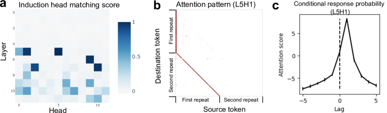
Figure 2: Induction heads in the GPT2-small model. (a) Several heads in GPT2 have a relatively large induction-head matching score. (b) The attention pattern of the L5H1 head, which has the largest induction-head matching score. The diagonal line (“induction stripe”) shows the attention from the destination token in the second repeat to the source token in the first repeat. (c) The attention scores of the L5H1 head averaged over all tokens in the designed prompt as a function of the relative position lag (similar to CRP). Error bars show the SEM across tokens.

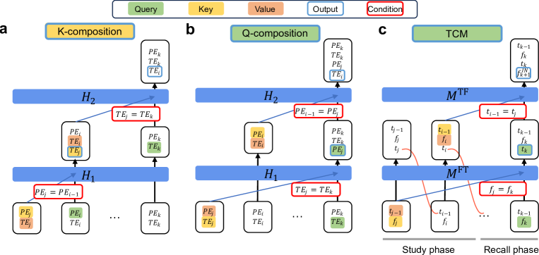
Figure 3: Comparison of composition mechanisms of induction heads and CMR. All panels correspond to the optimal Q-K match condition ($j=i-1$). See the main text and Tab. S2 for details. (a) K-composition induction head. The first-layer head’s output serves as the Key of the second-layer head. (b) Q-composition induction head. The first-layer head’s output serves as the Query of the second-layer head. (c) CMR is similar to a Q-composition induction head, except that the context vector $t_{j-1}$ is first updated by $M^{\rm FT}$ into $t_{j}$ at position $j$, then directly used at position $j+1$ (equal to $i$ for the optimal match condition; shown by red lines).

3.3 K-composition and Q-composition induction heads

Both the matching score and the copying score are useful to describe the behavior of individual attention heads; however, they do not provide a mechanistic understanding of how an induction head works internally. To gain some insights into the internal mechanisms of induction heads, we focus here on smaller transformer models, acknowledging that individual attention heads of LLMs likely exhibit more sophisticated behavior. Prior work has discovered two kinds of induction mechanisms in two-layer attention-only Transformer models: K-composition and Q-composition (Fig. 3a-b, Tab. tab:comparison) [19, 21], characterizing how information from the first-layer head is composed to inform attention of the second-layer head.

In K-composition (Fig. 3a), the first-layer “previous token” head uses the current token’s position embedding, $PE_{i}$, as the query, and a past token’s position embedding $PE_{j}$, as the key. When the match condition $PE_{j}=PE_{i-1}$ is satisfied (meaning $j$ is the previous position of $i$), the head writes the previous token’s token embedding, $TE_{j}$, as the value into the residual stream $z_{i}$. The second-layer induction head uses the current token’s $TE_{k}$ as the query, and the previous token head’s output $TE_{j}$ at residual stream $z_{i}$ as the key (“K-composition”). When the match condition $TE_{j}=TE_{k}$ is satisfied, the head writes $TE_{i}$ (at residual stream $z_{i}$) as the value into the residual stream $z_{k}$, effectively increasing the logit for the token that occurred at position $i$.

In Q-composition (Fig. 3b), the first-layer “duplicate token” head uses the current token’s $TE_{k}$ as the query, and a past token’s $TE_{j}$ as the key. When the match condition $TE_{j}=TE_{k}$ is satisfied (meaning token $k$ is a duplicate of token $j$), the head writes the token’s $PE_{j}$ as the value into the residual stream $z_{k}$. The second-layer induction head uses the duplicate token head’s output $PE_{j}$ at residual stream $z_{k}$ as the query (“Q-composition”) and a past token’s $PE_{i}$ as the key. When the match condition $PE_{j}=PE_{i-1}$ is satisfied, the head writes $TE_{i}$ (at residual stream $z_{i}$) as the value into the residual stream $z_{k}$, increasing the logit for the token that occurred at position $i$.

In the following sections, we will reveal a novel connection between ICL and human episodic memory. We first introduce the CMR model of episodic memory, and then formally re-write it as a Q-composition induction head performing prefix matching, allowing us to link induction heads’ attention biases to those known in human episodic memory.

4 Contextual maintenance and retrieval model (CMR)

4.1 CMR in its original form

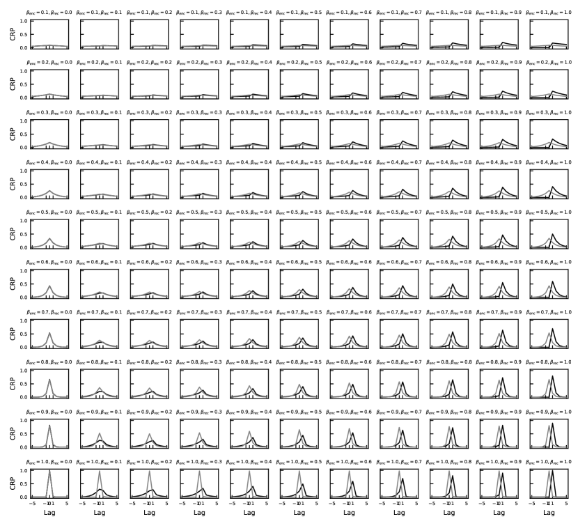
Figure S1: Example conditional response probability distributions produced by different parameterizations of CMR. Black lines correspond to $\gamma_{\rm FT}=0$ (i.e., only the pre-experimental contexts are used during retrieval). Grey lines correspond to $\gamma_{\rm FT}=1$ (i.e., only the experimental contexts are used during retrieval).

CMR, an influential model of human episodic memory, provides a general framework to model memory recall as association retrieval. It leverages a distributed representation called temporal context to guide sequential information retrieval [23]. CMR explains the asymmetric contiguity bias in human free recall (see Fig. 4 and Fig. S1) and has been extended to more complex memory phenomena such as semantic [24] and emotional [25] effects. Prior studies have suggested the entorhinal cortex and the hippocampus as potential biological infrastructures that support CMR and spatiotemporal relational learning [26]. CMR has been further related to the underlying mechanisms of flexible reinforcement learning and decision making [27, 28].

In CMR (Fig. 1d), each word token is represented by an embedding vector $\mathbf{f}$ (e.g., one-hot; $\mathbf{f}_{i}$ for the $i$-th word in a sequence). The core dynamic that drives both sequential encoding and retrieval is

$$\mathbf{t}_{i}=\rho\mathbf{t}_{i-1}+\beta\mathbf{t}^{\rm IN}_{i},$$ (1)

where $\mathbf{t}_{i}$ is the temporal context at time step $i$, and $\mathbf{t}^{\rm IN}_{i}$ is an input context associated with $\mathbf{f}_{i}$. $\beta$ controls the degree of temporal drift between time steps ($\beta_{\rm enc}$ for encoding (study) phase and $\beta_{\rm rec}$ for recall phase) and $\rho$ is picked to ensure $\mathbf{t}_{i}$ has unit norm. Specifically, during the encoding phase, $\mathbf{t}^{\rm IN}_{i}$ represents a pre-experimental context associated with the $i$-th word as $\mathbf{t}^{\rm IN}_{i}=\mathbf{M}^{\rm FT}_{\rm pre}\mathbf{f}_{i}$, where $\mathbf{M}^{\rm FT}_{\rm pre}$ is a pre-fixed matrix. At each time step, a word-to-context (mapping $\mathbf{f}$ to $\mathbf{t}$) memory matrix $\mathbf{M}^{\rm FT}_{\rm exp}$ learns the association between $\mathbf{f}_{i}$ and $\mathbf{t}_{i-1}$ (i.e., $\mathbf{M}^{\rm FT}_{\rm exp}$ is updated by $\mathbf{t}_{i-1}\mathbf{f}_{i}^{T}$). During the decoding (retrieval) phase, $\mathbf{t}^{\rm IN}_{i}$ is a mixture of pre-experimental ($\mathbf{t}_{\rm pre}^{\rm IN}=\mathbf{M}^{\rm FT}_{\rm pre}\mathbf{f}_{i}$) and experimental contexts ($\mathbf{t}_{\rm exp}^{\rm IN}=\mathbf{M}^{\rm FT}_{\rm exp}\mathbf{f}_{i}$). The proportion of these two contexts is controlled by an additional parameter $\gamma_{\rm FT}\in[0,1]$ as $\mathbf{t}^{\rm IN}_{i}=((1-\gamma_{\rm FT})\mathbf{M}^{\rm FT}_{\rm pre}+\gamma_{\rm FT}\mathbf{M}^{\rm FT}_{\rm exp})\mathbf{f}_{i}.$ The asymmetric contiguity bias arises from this slow evolution of temporal context: when $0<\beta<1$, $\mathbf{t}_{i}$ passes through multiple time steps, causing nearby tokens to be associated with temporally adjacent contexts that are similar to each other (temporal contiguity), i.e., $\langle\mathbf{t}_{i},\mathbf{t}_{j}\rangle$ is large if $|i-j|$ is small. Additionally, $\mathbf{t}_{\rm pre}^{\rm IN}=\mathbf{M}^{\rm FT}_{\rm exp}\mathbf{f}_{i}$ only enters the temporal context after time $i$. Thus $\mathbf{t}_{i,\rm exp}^{\rm IN}$ is associated with $\mathbf{f}_{j}$ only for $j>i$ (asymmetry).

CMR also learns a second context-to-word (mapping $\mathbf{t}$ back to $\mathbf{f}$) memory matrix $\mathbf{M}^{\rm TF}$ (updated by each $\mathbf{f}_{i}\mathbf{t}_{i-1}^{T}$). When an output is needed, CMR retrieves a mixed word embedding $\mathbf{f}_{i}^{\rm IN}=\mathbf{M}^{\rm TF}\mathbf{t}_{i}$. If $\mathbf{f}_{j}$ are one-hot encoded, we can simply treat $\mathbf{f}^{\rm IN}_{i}$ as a (unnormalized) probability distribution over the input tokens. Or, CMR can compute the inner product $\langle\mathbf{f}_{j},\mathbf{f}_{i}^{\rm IN}\rangle$ for each cached word $\mathbf{f}_{j}$ as input to softmax (with an inverse temperature $\tau^{-1}$) to recall a word.

Intuitively, the temporal context resembles a moving spotlight with a fuzzy edge: it carries recency-weighted historical information that may be relevant to the present, where the degree of information degradation is controlled by $\rho$. Larger $\beta$’s correspond to “sharper” CRPs with stronger forward asymmetry and stronger temporal clustering that are core features of human episodic memory. As a concrete example, consider $n$ unique one-hot encoded words $\{\mathbf{f}_{i}\}$. If $\mathbf{M}^{\rm FT}_{\rm pre}=\sum_{i=1}^{n}\mathbf{f}_{i}\mathbf{f}_{i}^{T}$ (i.e., the pre-experimental context associated with each word embedding is the word embedding itself) and $\gamma_{\rm FT}=0$, Eq. 1 at decoding is reduced to $\mathbf{t}_{i}=\rho\mathbf{t}_{i-1}+\beta\mathbf{f}_{i}=\sum_{j=1}^{i}\beta\rho^{i-j}\mathbf{f}_{j}$, which is a linear combination of past word embeddings.

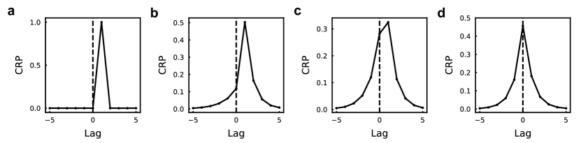
Figure 4: The conditional response probability (CRP) as a function of position lags given different parameter values for CMR. (a) CMR with “sequential chaining” behavior ($\beta_{\rm enc}=\beta_{\rm rec}=1,\gamma_{\rm FT}=0$). The recall has exactly the same order as the study phase without skipping over any word. (b) CMR with moderate updating at both encoding and retrieval, resulting in human-like free recall behavior ($\beta_{\rm enc}=\beta_{\rm rec}=0.7,\gamma_{\rm FT}=0$). Recall is more likely than not to have the same order as during study and sometimes skips words. (c-d) Same as (b) except with $\gamma_{\rm FT}=0.5$ (c) and $\gamma_{\rm FT}=1$ (d). For more examples, see Fig. S1.

4.2 CMR as an induction head

We now proceed to map CMR to a Q-composition-like head (see Fig. 3c and Tab. S2 for details).

(1) The word $\mathbf{f}_{i}$ seen at position $i$ is the same as $TE_{i}$.

(2) The context vector $\mathbf{t}_{i-1}$ (before update) at position $i$ is functionally similar to $PE_{i}$.

(3) The set {$\mathbf{f}_{i}$, $\mathbf{t}_{i-1}$} is functionally similar to the residual stream $z_{i}$, updated by the head outputs.

(4) CMR input-context retrieval resembles the first-layer self-attention. The temporal context is updated by $\mathbf{t}^{\rm IN}_{i}=((1-\gamma_{\rm FT})\mathbf{M}^{\rm FT}_{\rm pre}+\gamma_{\rm FT}\mathbf{M}^{\rm FT}_{\rm exp})\mathbf{f}_{i}$ at decoding. The memory matrix $\mathbf{M}_{\text{exp},i}^{\rm FT}$ acts as a first-layer duplicate token head, where the current word $\mathbf{f}_{i}$ is the query, the past embeddings $\{\mathbf{f}_{j}\}$ make up the keys, and the temporal contexts $\mathbf{t}_{j-1}$ associated with each $\mathbf{f}_{j}$ are values. This head effectively outputs “What’s the position (context vector) at which I encountered the same token $\mathbf{f}_{i}$?”

(5) The pre-experimental context $\mathbf{t}^{\rm IN}_{i}=\mathbf{M}^{\rm FT}_{\rm pre}\mathbf{f}_{i}$ (retrieved contextual information not present in the experiment) is the output of a linear fully-connected layer (functionally similar to MLP; not drawn).

(6) CMR evolution: the context vector is updated by $\mathbf{t}_{k}=\rho\mathbf{t}_{k-1}+\beta\mathbf{t}^{\rm IN}_{k}$. Equivalently, the head $\mathbf{M}^{\rm FT}$ updates the information from {$\mathbf{f}_{k}$, $\mathbf{t}_{k-1}$} to {$\mathbf{f}_{k}$, $\mathbf{t}_{k-1}$, $\mathbf{t}_{k}$}. At the position $k$ during recall, the updated context $\mathbf{t}_{k}$ contains $\mathbf{t}^{\rm IN}_{k}$ ($\approx\mathbf{t}_{j}$) (Fig. 3c).

(7) CMR context-word retrieval is akin to the second-layer self-attention. The retrieved embedding is $\mathbf{f}^{\rm IN}_{k}=\mathbf{M}^{\rm TF}\mathbf{t}_{k}$, where $\mathbf{M}^{\rm TF}$ acts as a second-layer induction head. In complement to point (4) above, now the temporal context $\mathbf{t}_{k}$ is the query, the past contexts $\{\mathbf{t}_{i-1}\}$ make up the keys, and the embeddings $\mathbf{f}_{i}$ associated with each $\mathbf{t}_{i-1}$ are values. This effectively implements Q-composition [19], because $\mathbf{t}_{k}$, as the Query, is affected by the output of the first-layer $\mathbf{M}^{\rm FT}$ head.

(8) CMR word recall: the final retrieved word probability is determined by the inner product between the retrieved memory $\mathbf{f}^{\rm IN}_{i}$ and each studied word $\mathbf{f}_{j}$, similar to the unembedding layer generating the output logits from the residual stream.

(9) The word-to-context matrix is updated by $\mathbf{M}_{\text{exp},i+1}^{\rm FT}=\mathbf{M}_{\text{exp},i}^{\rm FT}+\mathbf{t}_{i-1}\mathbf{f}_{i}^{T}$ (with $\mathbf{M}_{\text{exp},0}^{\rm FT}=\mathbf{0}$), associating $\mathbf{f}_{i}$ (key) and $\mathbf{t}_{i-1}$ (value). It is equivalent to a causal linear attention head, because $\mathbf{M}_{\text{exp}}^{\rm FT}\mathbf{f}_{k}=(\sum_{i<k}\mathbf{t}_{i-1}\mathbf{f}_{i}^{T})\mathbf{f_{k}}=\sum_{i<k}\mathbf{t}_{i-1}(\mathbf{f}_{i}^{T}\mathbf{f_{k}})=\sum_{i<k}\text{sim}(\mathbf{f}_{i},\mathbf{f_{k}})\mathbf{t}_{i-1}$.

(10) The context-to-word matrix, updated by $\mathbf{M}_{i+1}^{\rm TF}=\mathbf{M}_{i}^{\rm TF}+\mathbf{f}_{i}\mathbf{t}_{i-1}^{T}$ (with $\mathbf{M}_{0}^{\rm TF}=\mathbf{0}$), is equivalent to a causal linear attention head, associating $\mathbf{t}_{i-1}$ (key) and $\mathbf{f}_{i}$ (value).

To summarize, the CMR architecture resembles a two-layer transformer with a Q-composition linear induction head. It’s worth noting that although we cast $\mathbf{t}_{i}$ as the position embedding, unlike position embeddings that permit parallel processing in Transformer models, $\mathbf{t}_{i}$ is recurrently updated in CMR (Eq. 1). It is possible that Transformer models might acquire induction heads with a similar circuit mechanism, where $\mathbf{t}_{i}$ corresponds to autoregressively updated context information in the residual stream that serves as the input for downstream attention heads.

5 Experiments

5.1 Quantifying the similarity between an induction head and CMR

We have shown that induction heads in pre-trained LLMs exhibit CMR-like attention biases (Fig. 2c, Fig. 5a-c) and further established the mechanistic similarity between induction heads and CMR (Fig. 3). To further quantify their behavioral similarity, we propose the metric CMR distance, the mean squared error (MSE) between the head’s average attention scores and its CMR-fitted scores (see Appendix B and Fig. 5a-d). In practice, we optimized the parameters $(\beta_{\rm enc},\beta_{\rm rec},\gamma_{\rm FT},\tau^{-1})$ for each head to minimize the MSE.

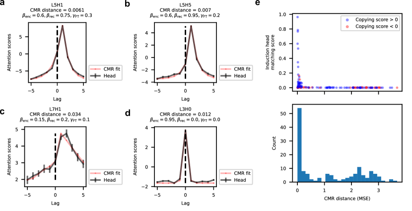
Figure 5: CMR distance provides meaningful descriptions for attention heads in GPT2. (a-c) Average attention scores and the CMR-fitted attention scores of example induction heads (with a non-zero induction-head matching score and positive copying score). (d) Average attention scores and the CMR-fitted attention scores of an example head that is traditionally not considered an induction head but can be well-captured by the CMR. (e) (Top) CMR distance (measured by MSE) and the induction-head matching score for each head. (Bottom) Histogram of the CMR distance.

At the population level, heads with a large induction-head matching score and a positive copying score also have a smaller CMR distance (Fig. 5e), suggesting that the CMR distance captures meaningful behavior of these heads. Notably, certain heads that are not typically considered induction heads (e.g., peaking at lag=0) can be well captured by CMR (Fig. 5d).

Consistent with prior findings that induction heads were primarily observed in the intermediate layers of LLMs [29], we found that the majority of heads in the intermediate layers of GPT2-small have lower CMR distances (Fig. 6a). We also replicated this result in a different set of LLMs called Pythia, a family of models with shared architecture but different sizes. While CMR-like heads tend to be more distributed in larger models (e.g., Pythia models with more than 1B parameters), they tend to distribute around 50%-80% relative layer positions in smaller LLMs (fewer than 1B parameters).

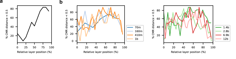
Figure 6: CMR distances vary with relative layer positions in LLMs. (a-b) Percentage of heads with a CMR distance less than 0.5 in different layers. (a) GPT2-small. (b) Pythia models across different model sizes (label indicates the number of model parameters). CMR distances are computed based on the last model checkpoint. Heads with lower CMR distances often emerge in the intermediate layers (more significant for smaller models).

5.2 CMR-like heads develop human-like temporal clustering over training

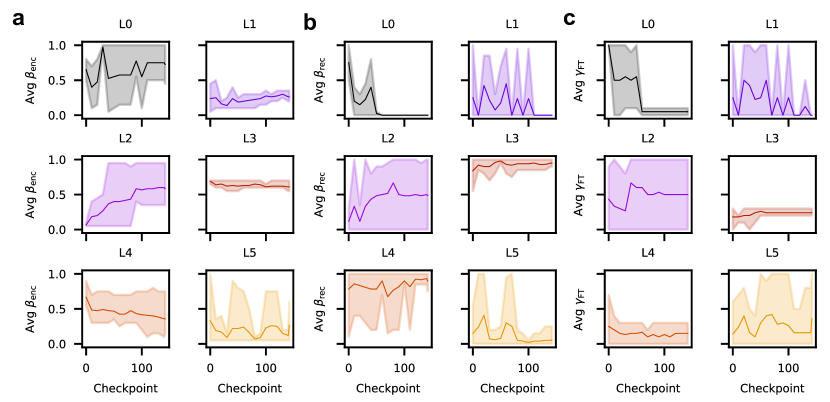
Figure S2: Fitted CMR parameters of Pythia-70m model over training. Solid lines indicate values averaged across heads with a CMR distance lower than 0.5 in the corresponding layer. Shaded areas indicate the range of fitted values (the lower edge indicates the minimum value; the upper edge indicates the maximum value). (a-b) Fitted CMR temporal drift parameters $\beta_{\rm enc}$ (a), and $\beta_{\rm rec}$ (b) in different layers as a function of training time. (c) Fitted experimental context mix parameter $\gamma_{\rm FT}$ in different layers as a function of training time.

As the model’s loss on the designed prompt decreases through training (Fig. 7a), the degree of temporal clustering increases, especially in layers where induction heads usually emerge. For instance, in the Pythia-70m model, heads in intermediate layers (e.g., L3, L4) show the strongest temporal clustering that persists over training compared to early and late layers (Fig. S2a-b). This, combined with an increasing inverse temperature (Fig. 7b), suggests that attention patterns become more deterministic over training, while shaped to mirror human-like asymmetric contiguity biases. In fact, human subjects with better free recall performance tend to exhibit stronger temporal clustering and a higher inverse temperature [30].

For individual heads, those with higher induction-head matching scores (Fig. 7c) (or similarly with smaller CMR distances, see Fig. 7e) consistently exhibit greater temporal clustering (Fig. 7d, f respectively), as the fitted $\beta$’s (both $\beta_{\rm enc}$ and $\beta_{\rm rec}$) were large. The fitted $\beta$’s of these attention heads fall into a similar range as human recall data (0.5-0.8) [31, 23, 32, 30]. We interpret this in light of a normative view of the human memory system: in humans, the asymmetric contiguity bias with a $\beta<1$ is not merely phenomenological; under the CMR framework, it gives rise to an optimal policy to maximize memory recall when encoding and retrieval are noisy [30]. In effect, a large $\beta$ (but less than 1) in Eq. 1 provides meaningful associations beyond adjacent words to facilitate recall, such that even if the immediately following token is poorly encoded or the agent fails to decode it, information from close-by tokens encapsulated in the temporal context still allows the agent to continue decoding.

In addition, we observed an increase in $\beta_{\rm enc}$ and $\beta_{\rm rec}$ (Fig. 7d, f) during the first 10 training checkpoints, when the model loss significantly drops. The increase in $\beta_{\rm rec}$ was particularly prominent, indicating the importance of temporal clustering during decoding for model performance. These results suggest that attention to temporally adjacent tokens with a contiguity bias – especially ones following the queried token (i.e., with asymmetry) – may support ICL in LLMs.

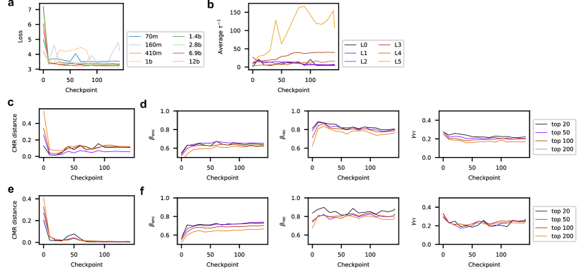
Figure 7: Strong asymmetric contiguity bias arises as model performance improves. (a) Model loss on the designed prompt as a function of training time. Loss is recorded every 10 training checkpoints. (b) Average fitted inverse temperature increases in the intermediate layers of Pythia-70m as training progresses. Values are averaged across heads with CMR distance lower than 0.5 in each layer. (c) CMR distance of top induction heads in Pythia models as a function of training time. Heads are selected based on the highest induction-head matching scores across all Pythia models (e.g., “top 20” corresponds to twenty heads with the highest induction-head matching scores). (d) Fitted CMR temporal drift parameters $\beta_{\rm enc}$(left), $\beta_{\rm rec}$ (middle), $\gamma_{\rm FT}$ (right) as a function of training time in attention heads with the highest induction-head matching scores. (e-f) Same as c-d but for top CMR-like heads (e.g., “top 20” corresponds to those with the lowest CMR distances).

6 Discussion

In this study, we have bridged the gap between LLMs and human episodic memory by comparing Transformer models’ induction heads and the CMR. We revealed the mechanistic similarities between CMR and Q-composition induction heads. We then probed CMR-like attention biases of heads in pre-trained LLMs, showing that induction heads manifest CMR’s asymmetric contiguity bias, a characteristic feature of human free recall. CMR-like behavior tends to appear in the intermediate layers of LLMs, and evolve towards a CMR state similar to that observed in human memory biases.

We have provided a fuller behavioral description and a novel reinterpretation of induction heads through the lens of CMR and the asymmetric contiguity bias in human episodic memory. Though CMR relies on recurrently updated context vectors that are mechanistically different from the K-composition and Q-composition heads, we speculate that deeper Transformer models might acquire similar mechanisms based on autoregressively updated information in the residual stream, a possibility yet to be researched. We further note that CMR-like heads are not exclusively induction heads – there are attention heads that do not fit into the conventional definition of an induction head yet can be well captured by CMR (e.g., Fig. 5d). Taken together, our results suggest an alternative view on the underlying mechanisms of ICL in LLMs, where heads may learn attention biases akin to human episodic memory to empower next-token prediction.

Our study is subject to several limitations. First, similar to previous works on induction heads, using the sequence of repeated random tokens as input to elicit induction behavior can overlook important functions of these heads in more natural language settings. Second, we use CMR to characterize these heads’ behavior, but whether it can serve as a mechanistic model of heads in larger Transformer models is unclear. Third, it is not clear whether our conclusions hold for other untested Transformer models. Addressing these limitations is one of our future directions.

Our findings open many possibilities for both fields. From the viewpoint of mechanistic interpretability, relating CMR to induction heads provides a novel approach to understanding these heads. For example, CMR not only applies to individual words but also to clusters of items [33], indicating potential roles of these heads in processing hierarchically organized, abstract chunks of texts. It has also been shown that Eq. 1 enables model-based action evaluation with sequential memory retrieval [28], suggesting similar roles of these heads in more complex cognitive functions. In addition, the “lost in the middle” phenomenon of LLMs’ attention on long contexts [34] is reminiscent of the well-known recency and primacy effects that are observed in human episodic memory and captured by CMR [17, 23], another phenomenological connection yet to be elucidated.

For the study of human episodic memory, the connection with induction heads might reveal normative principles of memory and hippocampal processing, echoing the view of the hippocampus as a future-predicting machine [35]. The core mechanisms of K-composition and Q-composition induction circuits might serve as alternative models to CMR, while further research is required to clarify whether they can explain experimental phenomena captured or not captured by CMR. K-composition and Q-composition require positional encoding, and we speculate that it can be similarly implemented by grid-like cells with periodic activations that track space and time [36]. It has been hypothesized that Transformers can be implemented in a biologically plausible way [37]. For a Transformer architecture, the MLP layers might be mapped to the cortex and the self-attention layers to the hippocampus. The model parameters could be encoded by slowly updated synapses in the cortex and hippocampus, and the key-value associations stored in fast Hebbian-like hippocampal synapses. The residual stream updated by MLP and attention layers may be akin to the activation-based working memory quickly updated by the cortico-hippocampal circuits. Our study therefore offers an important perspective to understand more general biological memory and hippocampal functions.

Appendix A Additional Experiment Details

A.1 Prompt design

The prompt is constructed by taking the top N=100 most common English tokens with a leading space (to avoid unwanted tokenization behavior), which are tokens with the largest biases in the unembedding layer of GPT2-small (or the Pythia models). The prompt concatenated two copies of the permuted word sequence and had a total length of $2N+1$ (one end-of-sequence token at the beginning). The two copies correspond to the study (encoding) and recall phases, respectively.

A.2 Experiment compute resources

The induction-head matching scores and copying scores of each head in GPT2-small and all Pythia models are computed using Google Colab Notebook. All models were pretrained and accessible through the TransformerLens library [22] with MIT License and used as is. See Table S1 for details.

Transformer Model	Type of compute worker	RAM (GB)	Storage (GB)	Computing time (minutes)
GPT2-small	CPU	12.7	225.8	$<1$
Pythia-70m-deduped-v0	CPU	12.7	225.8	2
Pythia-160m-deduped-v0	CPU	12.7	225.8	5
Pythia-410m-deduped-v0	CPU	12.7	225.8	15
Pythia-1b-deduped-v0	CPU	12.7	225.8	45
Pythia-1.4b-deduped-v0	High-RAM CPU	51.0	225.8	56
Pythia-2.8b-deduped-v0	High-RAM CPU	51.0	225.8	161
Pythia-6.9b-deduped-v0	TPU v2	334.6	225.3	111
Pythia-12b-deduped-v0	TPU v2	334.6	225.3	205

Table S1: Details of compute resources used to compute induction head metrics. All models were pretrained and accessible through the TransformerLens library [22] with MIT License. The numbers in the “Computing time” column indicate the total number of minutes it took to compute all scores for all heads across all checkpoints (except GPT2-small, which was not checkpointed, so only the final pre-trained model was evaluated).

We used an internal cluster to compute the subset of $\mathbf{q}$ (CRP) for model fitting. The internal cluster has 6 nodes with Dual Xeon E5-2699v3, which has 72 threads and 256GB RAM per thread, plus 4 nodes with Dual Xeon E5-2699v3, which has 72 threads and 512GB RAM per thread. This computation took a total of 90 hours.

Finally, model fitting was done on a 2023 MacBook Pro with 16GB RAM. All experiments were completed within 1 hour regardless of model size. This section contains all experiments we conducted that required non-trivial computational resources.

Appendix B Metrics & Definitions

B.1 Metrics for induction heads

Formally, we define the induction-head target pattern (i.e., attention probability distribution of an ideal induction head) $\mathbf{\bar{A}}=(\bar{a}_{d,s})$ over a sequence of tokens $\{x_{i}\}$ as

$$\bar{a}_{d,s}=\begin{cases}1,&\text{if $x_{s-1}=x_{d}$ and $s<d$}\\ 0,&\text{otherwise}\end{cases}.$$

Here, $d$ is the destination position and $s$ is the source position. We then assess the extent to which each attention head performs this kind of prefix matching [13, 22]. Specifically, the induction-head matching score for a head with attention pattern $\mathbf{A}=(a_{d,s})$ is defined as

$$(\sum_{d}\sum_{s}a_{d,s}\bar{a}_{d,s})/(\sum_{d}\sum_{s}a_{d,s})\in[0,1]$$

(Fig. 2a-b). A head that always performs ideal prefix matching will have an induction-head matching score of 1.

Additionally, an induction head should write to the current residual stream to increase the corresponding logit of the attended token (token copying). We adopt the copying score [19] to measure each head’s tendency of token copying. In particular, consider the circuit $W=W_{U}W_{O}W_{V}W_{E}$ for one head, where $W_{E}$ defines token embeddings, $W_{V}$ computes the value of each token from the residual stream (i.e., aggregated outputs from all earlier layers), $W_{O}$ computes the head’s output using a linear combination of the value vectors and the head’s attention pattern, and $W_{U}$ unembeds the output to predict the next token. The copying score of the head is equal to

$$(\sum_{k}\lambda_{k})/(\sum_{k}|\lambda_{k}|)\in[-1,1],$$

where ${\lambda_{k}}$’s are the eigenvalues of the matrix $W$. Since copying requires positive eigenvalues (corresponding to increased logits), an induction head should have a positive copying score. An ideal induction head will have a copying score of 1.

B.2 CRP analysis of attention heads

For a head with attention scores $\mathbf{\tilde{A}}$, the average attention score $\tilde{\alpha}_{\text{lag}}$ is defined as

$$\tilde{\alpha}_{\text{lag}}=\frac{1}{N-|\text{lag}|*2}\sum_{|\text{lag}|<s\leq N-|\text{lag}|}\tilde{a}_{s+N,s+\text{lag}},$$

where $N$ is the length of the first repeat in the prompt. Thus if $\text{lag}=0$, $\tilde{\alpha}_{\text{lag}}$ quantifies how much the first instance of a token is attended to on average; for $\text{lag}=1$, $\tilde{\alpha}_{\text{lag}}$ quantifies the average amount of attention distributed to the immediately following token in the first repeat. We used $\text{lag}\in[-5,5]$ throughout the paper.

B.3 CMR distance

The metric CMR distance is defined as

$$d_{\rm CMR}=\min_{\mathbf{q}}\left\{\sum_{\text{lag}}(q_{\text{lag}}-\tilde{\alpha}_{\text{lag}})^{2}/N_{\text{lag}}\right\}.$$

Here, $N_{\text{lag}}$ is the number of distinct lags, and $q_{\text{lag}}$ is obtained by calculating the CRP using CMR with specific parameter values. Note we did not consider the full set of possible $\mathbf{q}$ but only the subset given by the combinations of parameters $\beta_{\rm enc}=0.05,0.1,\dots,1$, $\beta_{\rm rec}=0,0.05,\dots,1$, and $\gamma_{\rm FT}=0,0.1,\dots,1$ for model fitting.

Appendix C Comparison of composition mechanisms of induction heads and CMR

		K-composition	Q-composition	CMR
Representation (residual stream) before $H_{1}$		$PE_{i}$ & $TE_{i}$ [At $i$] $PE_{j}$ & $TE_{j}$ [At $j$] $PE_{k}$ & $TE_{k}$ [At $k$]	$PE_{i}$ & $TE_{i}$ [At $i$] $PE_{j}$ & $TE_{j}$ [At $j$] $PE_{k}$ & $TE_{k}$ [At $k$]	$t_{i-1}$ & $f_{i}$ [At $i$] $t_{j-1}$ & $f_{j}$ [At $j$] $t_{k-1}$ & $f_{k}$ [At $k$]
First-layer head $H_{1}$	Type	previous token head	duplicate token head	word-to-context matrix $M^{\rm FT}$
	Query	$PE_{i}$ [At $i$]	$TE_{k}$ [At $k$]	$f_{k}$ [At $k$]
	Key	$PE_{j}$ [At $j$]	$TE_{j}$ [At $j$]	$f_{j}$ [At $j$]
	Optimal Q-K match condition	$PE_{j+1}=PE_{i}$	$TE_{j}=TE_{k}$	$f_{j}=f_{k}$
	Activation	Softmax	Softmax	Linear
	Value	$TE_{j}$ [At $j$]	$PE_{j}$ [At $j$]	$t_{j-1}$ [At $j$]
	Output	0 $TE_{j}$ [At $i$]∗	0 $PE_{j}$ [At $k$]∗	0 $t_{j-1}$ [At $k$]
Representation (residual stream) after $H_{1}$		$PE_{i}$ & $TE_{i}$ & $TE_{j}$ [At $i$] $PE_{j}$ & $TE_{j}$ [At $j$] $PE_{k}$ & $TE_{k}$ [At $k$]	$PE_{i}$ & $TE_{i}$ [At $i$] $PE_{j}$ & $TE_{j}$ [At $j$] $PE_{k}$ & $TE_{k}$ & $PE_{j}$ [At $k$]	$t_{i-1}$ & $t_{i}$ & $f_{i}$ [At $i$] $t_{j-1}$ & $t_{j}$ & $f_{j}$ [At $j$] $t_{k-1}$ & $t_{k}$ & $f_{k}$ [At $k$] †
second-layer head $H_{2}$	Type	induction head	induction head	context-to-word matrix $M^{\rm TF}$
	Query	$TE_{k}$ [At $k$]	0 $PE_{j}$ [At $k$]	0 $t_{j}$ [At $k$]†
	Key	0 $TE_{j}$ [At $i$]	$PE_{i}$ [At $i$]	$t_{i-1}$ [At $i$]
	Optimal Q-K match condition	$TE_{j}=TE_{k}$	$PE_{j+1}=PE_{i}$ ††	$t_{j}=t_{i-1}$ ††
	Activation	Softmax	Softmax	Linear
	Value	$TE_{i}$ [At $i$]	$TE_{i}$ [At $i$]	$f_{i}$ [At $i$]
	Output	$TE_{i}$ [At $k$]∗	$TE_{i}$ [At $k$]∗	$f_{k+1}^{\rm IN}$ [At $k$]
Representation (residual stream) after $H_{2}$		$PE_{i}$ & $TE_{i}$ & $TE_{j}$ [At $i$] $PE_{j}$ & $TE_{j}$ [At $j$] $PE_{k}$ & $TE_{k}$ & $TE_{i}$ [At $k$]	$PE_{i}$ & $TE_{i}$ [At $i$] $PE_{j}$ & $TE_{j}$ [At $j$] $PE_{k}$ & $TE_{k}$ & $PE_{j}$ & $TE_{i}$ [At $k$]	$t_{i-1}$ & $t_{i}$ & $f_{i}$ [At $i$] $t_{j-1}$ & $t_{j}$ & $f_{j}$ [At $j$] $t_{k-1}$ & $t_{k}$ & $f_{k}$ & $f_{k+1}^{\rm IN}$ [At $k$]

Table S2: Comparison of mechanisms of induction heads and CMR.
$PE_{i}$: position embedding for the token at index/position $i$.
$TE_{i}$: token embedding for the token at index/position $i$.
$t_{i-1}$: context vector associated with the word at index/position $i$.
$f_{i}$: word embedding for the word at index/position $i$.
$[\text{At }i]$: information available at index/position $i$.
^∗: The output is approximate (due to the weighted-average over all previous tokens).
^†: $t_{k}$ is updated from $t_{k-1}$ by $t_{j-1}$ (due to $M^{\rm FT}_{\rm exp}$) and $t_{j}^{\rm IN}$ (due to $M^{\rm FT}_{\rm pre}$), thus containing the information of $t_{j}$ (updated from $t_{j-1}$ by $t_{j}^{\rm IN}$).
^††: The optimal Q-K match condition in Q-composition requires transformation from $PE_{j}$ to $PE_{j+1}$, implemented by the $W_{Q}W_{K}$ matrix of $H_{2}$. The optimal Q-K match condition in CMR requires transformation from $t_{j-1}$ to $t_{j}$, implemented by $t^{\rm IN}_{\rm pre}$.

Appendix D Additional Figures

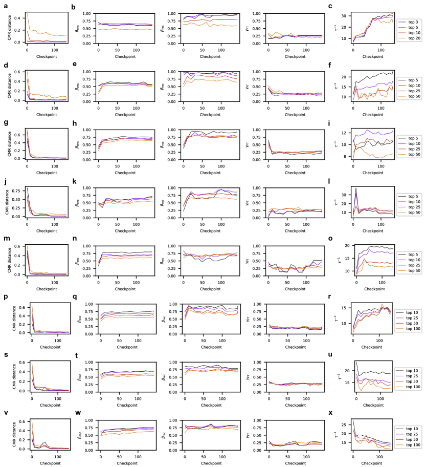
Figure S3: Behavior of top attention heads in different Pythia models. (a) CMR distance of the top CMR-like heads in Pythia-70m as a function of training time. Heads are selected by ranking all attention heads by their CMR distances (e.g., “top 3” heads correspond to the three lowest CMR distances). (b) Fitted CMR temporal drift parameters $\beta_{enc}$(left), $\beta_{rec}$ (middle), $\gamma_{\rm FT}$ (right) of the top CMR-like heads in Pythia-70m as a function of training time. (c) Average fitted inverse temperature of the top CMR-like heads in Pythia-70m as a function of training time. (d-x) Same as a-c except for Pythia-160m (d-f), Pythia-410m (g-i), Pythia-1b (j-l), Pythia-1.4b (m-o), Pythia-2.8b (p-r), Pythia-6.9b (s-u), and Pythia-12b (v-x).

References

- Yamins et al. [2014] Daniel LK Yamins, Ha Hong, Charles F Cadieu, Ethan A Solomon, Darren Seibert, and James J DiCarlo. Performance-optimized hierarchical models predict neural responses in higher visual cortex. Proceedings of the national academy of sciences, 111(23):8619–8624, 2014.
- Yamins and DiCarlo [2016] Daniel LK Yamins and James J DiCarlo. Using goal-driven deep learning models to understand sensory cortex. Nature neuroscience, 19(3):356–365, 2016.
- Schrimpf et al. [2018] Martin Schrimpf, Jonas Kubilius, Ha Hong, Najib J Majaj, Rishi Rajalingham, Elias B Issa, Kohitij Kar, Pouya Bashivan, Jonathan Prescott-Roy, Franziska Geiger, et al. Brain-score: Which artificial neural network for object recognition is most brain-like? BioRxiv, page 407007, 2018.
- Cueva and Wei [2018] Christopher J Cueva and Xue-Xin Wei. Emergence of grid-like representations by training recurrent neural networks to perform spatial localization. arXiv preprint arXiv:1803.07770, 2018.
- Banino et al. [2018] Andrea Banino, Caswell Barry, Benigno Uria, Charles Blundell, Timothy Lillicrap, Piotr Mirowski, Alexander Pritzel, Martin J Chadwick, Thomas Degris, Joseph Modayil, et al. Vector-based navigation using grid-like representations in artificial agents. Nature, 557(7705):429–433, 2018.
- Wang et al. [2018] Jane X Wang, Zeb Kurth-Nelson, Dharshan Kumaran, Dhruva Tirumala, Hubert Soyer, Joel Z Leibo, Demis Hassabis, and Matthew Botvinick. Prefrontal cortex as a meta-reinforcement learning system. Nature neuroscience, 21(6):860–868, 2018.
- Hanson et al. [2018] Catherine Hanson, Leyla Roskan Çağlar, and Stephen José Hanson. Attentional bias in human category learning: The case of deep learning. Frontiers in Psychology, 9, 2018. URL https://api.semanticscholar.org/CorpusID:4789239.
- Vaswani et al. [2017] Ashish Vaswani, Noam Shazeer, Niki Parmar, Jakob Uszkoreit, Llion Jones, Aidan N. Gomez, Lukasz Kaiser, and Illia Polosukhin. Attention is all you need. In Isabelle Guyon, Ulrike von Luxburg, Samy Bengio, Hanna M. Wallach, Rob Fergus, S. V. N. Vishwanathan, and Roman Garnett, editors, Advances in Neural Information Processing Systems 30: Annual Conference on Neural Information Processing Systems 2017, December 4-9, 2017, Long Beach, CA, USA, pages 5998–6008, 2017. URL https://proceedings.neurips.cc/paper/2017/hash/3f5ee243547dee91fbd053c1c4a845aa-Abstract.html.
- Goldstein et al. [2024] Ariel Goldstein, Avigail Grinstein-Dabush, Mariano Schain, Haocheng Wang, Zhuoqiao Hong, Bobbi Aubrey, Mariano Schain, Samuel A Nastase, Zaid Zada, Eric Ham, et al. Alignment of brain embeddings and artificial contextual embeddings in natural language points to common geometric patterns. Nature communications, 15(1):2768, 2024.
- Schrimpf et al. [2020] Martin Schrimpf, Idan Blank, Greta Tuckute, Carina Kauf, Eghbal A Hosseini, Nancy Kanwisher, Joshua Tenenbaum, and Evelina Fedorenko. The neural architecture of language: Integrative reverse-engineering converges on a model for predictive processing. BioRxiv, 2020.
- Antonello et al. [2024] Richard Antonello, Aditya Vaidya, and Alexander Huth. Scaling laws for language encoding models in fmri. Advances in Neural Information Processing Systems, 36, 2024.
- Whittington et al. [2021] James CR Whittington, Joseph Warren, and Timothy EJ Behrens. Relating transformers to models and neural representations of the hippocampal formation. arXiv preprint arXiv:2112.04035, 2021.
- Olsson et al. [2022] Catherine Olsson, Nelson Elhage, Neel Nanda, Nicholas Joseph, Nova DasSarma, Tom Henighan, Ben Mann, Amanda Askell, Yuntao Bai, Anna Chen, et al. In-context learning and induction heads. arXiv preprint arXiv:2209.11895, 2022.
- Radford et al. [2019] Alec Radford, Jeffrey Wu, Rewon Child, David Luan, Dario Amodei, Ilya Sutskever, et al. Language models are unsupervised multitask learners. OpenAI blog, 1(8):9, 2019.
- Brown et al. [2020] Tom Brown, Benjamin Mann, Nick Ryder, Melanie Subbiah, Jared D Kaplan, Prafulla Dhariwal, Arvind Neelakantan, Pranav Shyam, Girish Sastry, Amanda Askell, et al. Language models are few-shot learners. Advances in neural information processing systems, 33:1877–1901, 2020.
- Murdock and Bennet [1962] Murdock and B Bennet. The serial position effect of free recall. Journal of Experimental Psychology, 64:482–488, 1962.
- Howard and Kahana [2002] Marc W Howard and Michael J Kahana. A distributed representation of temporal context. Journal of mathematical psychology, 46(3):269–299, 2002.
- Ratcliff and McKoon [1981] Roger Ratcliff and Gail McKoon. Does activation really spread? Psychological Review, 88(5):454–462, 1981. doi: 10.1037/0033-295x.88.5.454.
- Elhage et al. [2021] Nelson Elhage, Neel Nanda, Catherine Olsson, Tom Henighan, Nicholas Joseph, Ben Mann, Amanda Askell, Yuntao Bai, Anna Chen, Tom Conerly, et al. A mathematical framework for transformer circuits. Transformer Circuits Thread, 1, 2021.
- Reddy [2023] Gautam Reddy. The mechanistic basis of data dependence and abrupt learning in an in-context classification task. arXiv preprint arXiv:2312.03002, 2023.
- Singh et al. [2024] Aaditya K Singh, Ted Moskovitz, Felix Hill, Stephanie CY Chan, and Andrew M Saxe. What needs to go right for an induction head? a mechanistic study of in-context learning circuits and their formation. arXiv preprint arXiv:2404.07129, 2024.
- Nanda [2022] Neel Nanda. Transformerlens, 2022. URL https://github.com/neelnanda-io/TransformerLens.
- Polyn et al. [2009] Sean M Polyn, Kenneth A Norman, and Michael J Kahana. A context maintenance and retrieval model of organizational processes in free recall. Psychological review, 116(1):129, 2009.
- Lohnas et al. [2015a] Lynn Lohnas, Sean Polyn, and Michael Kahana. Expanding the scope of memory search: Modeling intralist and interlist effects in free recall. Psychological review, 122:337–363, 04 2015a. doi: 10.1037/a0039036.
- Cohen and Kahana [2019] Rivka T Cohen and Michael J. Kahana. Retrieved-context theory of memory in emotional disorders. bioRxiv, page 817486, 2019.
- Howard et al. [2005] Marc W Howard, Mrigankka S Fotedar, Aditya V Datey, and Michael E. Hasselmo. The temporal context model in spatial navigation and relational learning: toward a common explanation of medial temporal lobe function across domains. Psychological review, 112 1:75–116, 2005. URL https://api.semanticscholar.org/CorpusID:16459919.
- Gershman et al. [2012] Samuel J Gershman, Christopher D Moore, Michael T Todd, Kenneth A Norman, and Per B Sederberg. The successor representation and temporal context. Neural Computation, 24(6):1553–1568, 2012.
- Zhou et al. [2023] Corey Y. Zhou, Deborah Talmi, Nathaniel D. Daw, and Marcelo G. Mattar. Episodic retrieval for model-based evaluation in sequential decision tasks, 2023. URL https://doi.org/10.31234/osf.io/3sqjh.
- Bansal et al. [2022] Hritik Bansal, Karthik Gopalakrishnan, Saket Dingliwal, S. Bodapati, Katrin Kirchhoff, and Dan Roth. Rethinking the role of scale for in-context learning: An interpretability-based case study at 66 billion scale. In Annual Meeting of the Association for Computational Linguistics, 2022.
- Zhang et al. [2023] Qiong Zhang, Thomas L. Griffiths, and Kenneth A. Norman. Optimal policies for free recall. Psychological Review, 130(4):1104–1124, 2023. doi: 10.1037/rev0000375.
- Sederberg et al. [2008] Per B. Sederberg, Marc W Howard, and Michael J. Kahana. A context-based theory of recency and contiguity in free recall. Psychological review, 115 4:893–912, 2008.
- Lohnas et al. [2015b] Lynn J. Lohnas, Sean M. Polyn, and Michael J. Kahana. Expanding the scope of memory search: Modeling intralist and interlist effects in free recall. Psychological review, 122(2):337–63, 2015b.
- Morton and Polyn [2016] Neal W Morton and Sean M Polyn. A predictive framework for evaluating models of semantic organization in free recall. Journal of memory and language, 86:119–140, 2016. doi: 10.1016/j.jml.2015.10.002.
- Liu et al. [2024] Nelson F Liu, Kevin Lin, John Hewitt, Ashwin Paranjape, Michele Bevilacqua, Fabio Petroni, and Percy Liang. Lost in the middle: How language models use long contexts. Transactions of the Association for Computational Linguistics, 12:157–173, 2024.
- Stachenfeld et al. [2017] Kimberly L Stachenfeld, Matthew M Botvinick, and Samuel J Gershman. The hippocampus as a predictive map. Nature neuroscience, 20(11):1643–1653, 2017.
- Kraus et al. [2015] Benjamin J Kraus, Mark P Brandon, Robert J Robinson, Michael A Connerney, Michael E Hasselmo, and Howard Eichenbaum. During running in place, grid cells integrate elapsed time and distance run. Neuron, 88(3):578–589, 2015.
- Kozachkov et al. [2023] Leo Kozachkov, Ksenia V Kastanenka, and Dmitry Krotov. Building transformers from neurons and astrocytes. Proceedings of the National Academy of Sciences, 120(34):e2219150120, 2023.