Linearized Boundary Control Method for Density Reconstruction in Acoustic Wave Equations

Abstract

We develop a linearized boundary control method for the inverse boundary value problem of determining a density in the acoustic wave equation. The objective is to reconstruct an unknown perturbation in a known background density from the linearized Neumann-to-Dirichlet map. A key ingredient in the derivation is a linearized Blagoves̆c̆enskiĭ’s identity with a free parameter. When the linearization is at a constant background density, we derive two reconstructive algorithms with stability estimates based on the boundary control method. When the linearization is at a non-constant background density, we establish an increasing stability estimate for the recovery of the density perturbation. The proposed reconstruction algorithms are implemented and validated with several numerical experiments to demonstrate the feasibility.

1 Introduction

The paper is concerned with the linearized inverse boundary value problem (IBVP) for the acoustic wave equation with a potential. The goal is to derive uniqueness, stability estimates and reconstruction procedures to numerically compute a small perturbation of a certain parameter in the wave equation from the knowledge of infinite boundary data. This parameter reduces to the slowness (i.e, reciprocal of the wave speed) in the absence of the potential.

Formulation. We begin with the formulation of the inverse boundary value problem for the wave equation. Let $T>0$ be a constant and $\Omega\subset\mathbb{R}^{n}$ be a bounded open subset with smooth boundary $\partial\Omega$. Consider the following boundary value problem for the acoustic wave equation with potential:

$$\left\{\begin{array}[]{rcl}\rho(x)\partial^{2}_{t}u(t,x)-\Delta u(t,x)+q(x)u(t,x)&=&0,\quad\quad\quad\text{ in }(0,2T)\times\Omega\\ \partial_{\nu}u&=&f,\quad\quad\quad\text{ on }(0,2T)\times\partial\Omega\\ u(0,x)=\partial_{t}u(0,x)&=&0\quad\quad\quad\quad x\in\Omega.\end{array}\right.$$ (1)

Here, $\rho(x)\in C^{\infty}(\overline{\Omega})$ is a positive smooth function that is strictly positive, $q(x)\in C^{\infty}(\overline{\Omega})$ is a real-valued function referred to as the potential. We write the wave solution as $u=u^{f}(t,x)$ whenever it is necessary to specify the Neumann data.

Given $f\in C^{\infty}_{c}((0,2T)\times\partial\Omega)$, the well-posedness of this problem is ensured by the standard theory for second order hyperbolic partial differential equations [14]. As a result, the following Neumann-to-Dirichlet map (ND map) is well defined:

$$\Lambda_{\rho}f:=u^{f}|_{(0,2T)\times\partial\Omega}.$$ (2)

Throughout the paper, we will fix a known potential $q$ and only study the dependence of the ND map on the parameter $\rho$. This dependence is indicated by the subscript. The inverse boundary value problem (IBVP) we are interested in concerns recovery of $\rho(x)$ from knowledge of the ND map $\Lambda_{\rho}$, that is, to invert the parameter-to-data map $\rho\mapsto\Lambda_{\rho}$.

Literature. The IBVP has been studied in the mathematical literature for a long time, and most of the results were obtained in the absence of the potential. When $q\equiv 0$, the parameter $\rho(x)$ is related to the wave speed $c(x)$ by $\rho(x)=c^{-2}(x)$. In this circumstance, the IBVP aims to recover the spatial distribution of the wave speed $c$. For $q\equiv 0$ and $c=c(x)$, Belishev [1] proved that $c$ (hence $\rho$) is uniquely determined using the boundary control (BC) method combined with Tataru’s unique continuation result [35, 36]. The method has since been extended to many wave equations. We mention [5] for a generalization to Riemannian manifolds, and [23] for a result covering all symmetric time-independent lower order perturbations of the wave operator. Non-symmetric, time-dependent and matrix-valued lower order perturbations were recovered in [12] [24], and [25], respectively. For a review of the BC method, we refer to [3, 20].

As for the stability, it can be proven that the IBVP to recover the wave speed $c$ is Hölder stable under suitable geometric assumptions [32, 33], even when the speed is anisotropic (hence represented by a Riemannian metric). On the other hand, a low-pass version of $c$ can be recovered with Lipschitz-type stability [27].

The BC method has been implemented numerically to reconstruct the wave speed $c$ in [2], and subsequently in [4, 11, 31, 37]. The implementations [2, 4, 11] involve solving unstable control problems, whereas [31, 37] are based on solving stable control problems but with target functions exhibiting exponential growth or decay. The exponential behaviour leads to instability as well. On the other hand, the linearized approach introduced in the present paper is stable. It should be mentioned that the BC method can be implemented in a stable way in the one-dimensional case, see [21]. For an interesting application of a variant of the method in the one-dimensional case, see [8] on detection of blockage in networks.

Formal Linearization. We are interested in the linearized IBVP in this paper. To this end, let us formally linearize the parameter-to-data map $\rho\mapsto\Lambda_{\rho}$. Recall that the potential $q$ is known and fixed. We write

$$\rho(x)=\rho_{0}(x)+\epsilon\dot{\rho}(x),\quad\quad u(t,x)=u_{0}(t,x)+\epsilon\dot{u}(t,x)$$

where $\rho_{0}$ is a known background potential and $u_{0}$ is the background solution, $\dot{\rho}\in C_{c}^{\infty}(\Omega)$ is a compactly supported smooth perturbation. Equating the $O(1)$-terms gives

$$\left\{\begin{array}[]{rcll}\rho_{0}(x)\partial^{2}_{t}u_{0}(t,x)-\Delta u_{0}(t,x)+q(x)u_{0}(t,x)&=&0,&\quad\text{ in }(0,2T)\times\Omega\\ \partial_{\nu}u_{0}&=&f,&\quad\text{ on }(0,2T)\times\partial\Omega\\ u_{0}(0,x)=\partial_{t}u_{0}(0,x)&=&0,&\quad x\in\Omega.\end{array}\right.$$ (3)

Equating the $O(\epsilon)$-terms gives

$$\left\{\begin{array}[]{rcll}\rho_{0}(x)\partial^{2}_{t}\dot{u}(t,x)-\Delta\dot{u}(t,x)+q(x)\dot{u}(t,x)&=&-\dot{\rho}\partial^{2}_{t}u_{0}(t,x),&\quad\text{ in }(0,2T)\times\Omega\\ \partial_{\nu}\dot{u}&=&0,&\quad\text{ on }(0,2T)\times\partial\Omega\\ \dot{u}(0,x)=\partial_{t}\dot{u}(0,x)&=&0&\quad x\in\Omega.\end{array}\right.$$ (4)

Correspondingly, we write the ND map as $\Lambda_{\rho}=\Lambda_{\rho_{0}}+\epsilon\dot{\Lambda}_{\dot{\rho}}$, where $\Lambda_{\rho_{0}}$ is the ND map for the unperturbed boundary value problem (3), and $\dot{\Lambda}_{\dot{\rho}}$ is defined as

$$\dot{\Lambda}_{\dot{\rho}}:f\mapsto\dot{u}|_{(0,2T)\times\partial\Omega}.$$ (5)

Note that the unperturbed problem (3) can be explicitly solved to obtain $u_{0}$ and $\Lambda_{\rho_{0}}$, since $\rho_{0}$ and $q$ are known. As before, we will write $\dot{u}=\dot{u}^{f}:=\dot{\Lambda}_{\dot{\rho}}f$ if it is necessary to specify the Neumann data $f$. The linearized IBVP concerns recovery of a compactly-supported smooth perturbation $\dot{\rho}\in C^{\infty}_{c}(\Omega)$ near a known $0<\rho_{0}\in C^{\infty}(\overline{\Omega})$ from the data $\dot{\Lambda}_{\dot{\rho}}$.

Contribution of the Paper. The major contribution of this paper consists of novel ideas to tackle linearized acoustic IBVPs as well as several results regarding the uniqueness, stability, and reconstructive algorithms. These include

• A linearized Blagoves̆c̆enskiĭ’s identity with a free parameter. The Blagoves̆c̆enskiĭ’s identity plays a central role in the boundary method by bridging boundary measurement with inner products of waves. For the linearized IBVP, the authors’ earlier work [30] derived a version of the linearized Blagoves̆c̆enskiĭ’s identity with a free parameter in the presence of a potential. The free parameter enlarges the class of testing functions that can be used to probe the unknown parameter, resulting in improved stability and reconstruction. In this paper, we derived another version of the linearized Blagoves̆c̆enskiĭ’s identity with a free parameter in the presence of a density, see Proposition 7. This identity forms the foundation for the derivation of other results.

• Multiple reconstruction formulae and algorithms to recover $\dot{\rho}$. Specifically: (1) For constant $\rho_{0}$ and $q\equiv 0$, we derive a reconstruction formula for $\dot{\rho}$ in Algorithm 1. This algorithm is numerically implemented and validated in 1D with quantitative assessment of the accuracy. Moreover, A pointwise stability estimate for the Fourier transform of $\dot{\rho}$ is established in Theorem 10. (2) For constant $\rho_{0}$ and $q\not\equiv 0$, we derive another reconstruction formula for $\dot{\rho}$ in Algorithm 2.

• An increasing stability estimate. For variable $\rho_{0}\in C^{\infty}(\overline{\Omega})$, we prove a stability estimate for the reconstruction of $\dot{\rho}$ in Theorem 13. This estimate contains the free parameter in the linearized Blagoves̆c̆enskiĭ’s identity. The stability is a blend of a Hölder-type stability and a log-type stability. However, as the free parameter increases, the log-type decreases, leading to a nearly Hölder-type stability. This phenomenon is known as the increasing stability, and has been studied in the frequency domain for the Helmholtz equation [9, 15, 16, 19, 17, 18, 22, 28]. In this paper, we make use of the linearized Blagoves̆c̆enskiĭ’s identity with a free parameter to establish an increasing stability result for the IBVP in the time domain, see Theorem 13. An interesting observation is that the free parameter plays the role of the frequency for the probing test functions.

Paper Structure. The paper is organized as follows. Section 2 reviews fundamental concepts and results in the BC method. Section 3 is devoted to the proof of an integral identity that is essential to the development of our linearized BC method. Section 4 establishes several stability estimates and reconstructive algorithms for the linearized IBVP, which are the main results of the paper. Section 5 consists of numerical implementation of a reconstruction formula as well as multiple numerical experiments for a proof-of-concept validation.

2 Preliminaries

Introduce some notations: Given a function $u(t,x)$, we write $u(t)=u(t,\cdot)$ for the spatial part as a function of $x$. Introduce the time reversal operator $R:L^{2}([0,T]\times\partial\Omega)\rightarrow L^{2}([0,T]\times\partial\Omega)$,

$$Ru(t,\cdot):=u(T-t,\cdot),\quad\quad 0<t<T;$$ (6)

and the low-pass filter $J:L^{2}([0,2T]\times\partial\Omega)\rightarrow L^{2}([0,T]\times\partial\Omega)$

$$Jf(t,\cdot):=\frac{1}{2}\int^{2T-t}_{t}f(\tau,\cdot)\,d\tau,\quad\quad 0<t<T.$$ (7)

Let $\mathcal{T}_{D}$ and $\mathcal{T}_{N}$ be the Dirichlet and Neumann trace operators respectively, that is,

$$\mathcal{T}_{D}u(t,\cdot)=u(t,\cdot)|_{\partial\Omega},\quad\quad\quad\mathcal{T}_{N}u(t,\cdot)=\partial_{\nu}u(t,\cdot)|_{\partial\Omega}.$$

We write $P_{T}:L^{2}([0,2T]\times\partial\Omega)\rightarrow L^{2}([0,T]\times\partial\Omega)$ for the orthogonal projection via restriction. Its adjoint operator $P^{*}_{T}:L^{2}([0,T]\times\partial\Omega)\rightarrow L^{2}([0,2T]\times\partial\Omega)$ is the extension by zero.

Introduce the connecting operator

$$K:=J\Lambda_{\rho}P^{\ast}_{T}-R\Lambda_{\rho,T}RJP^{\ast}_{T}$$ (8)

where $\Lambda_{\rho,T}f:=P_{T}\Lambda_{\rho}P^{*}_{T}f$. Then the following Blagoves̆c̆enskiĭ’s identity holds [6, 7, 10, 29].

Proposition 1.

Let $u^{P^{*}_{T}f},u^{P^{*}_{T}h}$ be the solutions of (1) with the Neumann traces $f,h\in L^{2}((0,T)\times\partial\Omega)$, respectively. Then

$$(\rho u^{P^{*}_{T}f}(T),u^{P^{*}_{T}h}(T))_{L^{2}(\Omega)}=(f,Kh)_{L^{2}((0,T)\times\partial\Omega)}=(Kf,h)_{L^{2}((0,T)\times\partial\Omega)}.$$ (9)

Proof.

We begin with the additional assumption that $f,h\in C^{\infty}_{c}((0,T)\times\partial\Omega)$. Define

$$I(t,s):=(\rho u^{P^{*}_{T}f}(t),u^{P^{*}_{T}h}(s))_{L^{2}(\Omega)}.$$

We compute

$$(\partial^{2}_{t}-\partial^{2}_{s})I(t,s)$$

$$= ((\Delta-q)u^{P^{*}_{T}f}(t),u^{P^{*}_{T}h}(s))_{L^{2}(\Omega)}-(u^{P^{*}_{T}f}(t),(\Delta-q)u^{P^{*}_{T}h}(s))_{L^{2}(\Omega)}$$

$$= (P^{*}_{T}f(t),\Lambda_{\rho}P^{*}_{T}h(s))_{L^{2}(\partial\Omega)}-(\Lambda_{\rho}P^{*}_{T}f(t),P^{*}_{T}h(s))_{L^{2}(\partial\Omega)},$$ (10)

where the last equality follows from the integration by parts. On the other hand, $I(0,s)=\partial_{t}I(0,s)=0$ since $u^{P^{*}_{T}f}(0,x)=\partial_{t}u^{P^{*}_{T}f}(0,x)=0$. Solve the inhomogeneous $1$D wave equation (10) together with these initial conditions to obtain

$$I(T,T) =\frac{1}{2}\int^{T}_{0}\int^{2T-t}_{t}\left[(P^{*}_{T}f(t),\Lambda_{\rho}P^{*}_{T}h(\sigma))_{L^{2}(\partial\Omega)}-(\Lambda_{\rho}P^{*}_{T}f(t),P^{*}_{T}h(\sigma))_{L^{2}(\partial\Omega)}\right]\,d\sigma dt\vspace{1ex}$$

$$=\int^{T}_{0}[(P^{*}_{T}f(t),\frac{1}{2}\int^{2T-t}_{t}\Lambda_{\rho}P^{*}_{T}h(\sigma)\,d\sigma)_{L^{2}(\partial\Omega)}-(\Lambda_{\rho}P^{*}_{T}f(t),\frac{1}{2}\int^{2T-t}_{t}P^{*}_{T}h(\sigma)\,d\sigma)_{L^{2}(\partial\Omega)}]\,dt\vspace{1ex}$$

$$=(f,J\Lambda_{\rho}P^{*}_{T}h)_{L^{2}((0,T)\times\partial\Omega)}-(P_{T}(\Lambda_{\rho}P^{*}_{T}f),JP^{*}_{T}h)_{L^{2}((0,T)\times\partial\Omega)}.$$

Using the relations $P_{T}(\Lambda_{\rho}P^{*}_{T}f)=\Lambda_{\rho,T}f$ and $\Lambda^{\ast}_{\rho,T}=R\Lambda_{\rho,T}R$ on $L^{2}((0,T)\times\partial\Omega)$, we have

$$I(T,T) =(f,J\Lambda_{\rho}P^{\ast}_{T}h)_{L^{2}((0,T)\times\partial\Omega)}-(\Lambda_{\rho,T}f,JP^{\ast}_{T}h)_{L^{2}((0,T)\times\partial\Omega)}$$

$$=(f,J\Lambda_{\rho}P^{\ast}_{T}h)_{L^{2}((0,T)\times\partial\Omega)}-(f,R\Lambda_{\rho,T}RJP^{\ast}_{T}h)_{L^{2}((0,T)\times\partial\Omega)}$$

$$=(f,Kh)_{L^{2}((0,T)\times\partial\Omega)}$$

For general $f,h\in L^{2}((0,T)\times\partial\Omega)$, notice that $K:L^{2}((0,T)\times\partial\Omega)\rightarrow L^{2}((0,T)\times\partial\Omega)$ is a continuous operator since all the operators in the definition (8) are continuous. The result follows from the density of compactly supported smooth functions in $L^{2}$. ∎

Remark 2.

The zero extension $P^{*}_{T}$ plays no special role than other extensions in Proposition 1. In fact, if $Q^{*}_{T}$ is another extension such that $P_{T}Q^{*}_{T}f=f$ for all $f\in L^{2}((0,T)\times\partial\Omega)$, then

$$u^{P^{*}_{T}f}=u^{Q^{*}_{T}f}\quad\text{ on }[0,T]\times\Omega$$

as they satisfy identical initial and boundary conditions on $[0,T]$. Because of this observation, we often omit the notation for extension and simply write $u^{P^{*}_{T}f}$ as $u^{f}$ and write $\dot{\Lambda}_{T}$ as $\dot{\Lambda}$ when considering functions on $[0,T]$.

Corollary 3.

Suppose $f,h\in C^{\infty}_{c}((0,T]\times\partial\Omega)$. Then

$$((\Delta-q)u^{f}(T),u^{h}(T))_{L^{2}(\Omega)}=(\partial^{2}_{t}f,Kh)_{L^{2}((0,T)\times\partial\Omega)}=(K\partial^{2}_{t}f,h)_{L^{2}((0,T)\times\partial\Omega)}.$$ (11)

Proof.

Replacing $f$ by $\partial^{2}_{t}f$ in (9), we get

$$(\rho u^{\partial^{2}_{t}f}(T),u^{h}(T))_{L^{2}(\Omega)}=(\partial^{2}_{t}f,Kh)_{L^{2}((0,T)\times\partial\Omega)}=(K\partial^{2}_{t}f,h)_{L^{2}((0,T)\times\partial\Omega)}.$$

As both $u^{\partial^{2}_{t}f}$ and $\partial^{2}_{t}u^{f}$ satisfy (1) with $f$ replaced by $\partial^{2}_{t}f$, they must be equal thanks to the well-posedness of the boundary value problem. We conclude

$$\rho u^{\partial^{2}_{t}f}=\rho\partial^{2}_{t}u^{f}=\Delta u^{f}-qu^{f}.$$

∎

Recall that $\Lambda_{\rho}=\Lambda_{\rho_{0}}+\epsilon\dot{\Lambda}_{\dot{\rho}}$ in the linearization setting. When there is no risk of confusion, we write $\dot{\Lambda}_{\dot{\rho}}$ simply as $\dot{\Lambda}$.

Accordingly, we decompose $K=K_{0}+\epsilon\dot{K}$. Here $K_{0}$ is the connecting operator for the background medium:

$$K_{0}:=J\Lambda_{\rho_{0}}P^{\ast}_{T}-R\Lambda_{\rho_{0},T}RJP^{\ast}_{T}.$$ (12)

$K_{0}$ can be explicitly computed since $\Lambda_{\rho_{0}}$ is known. $\dot{K}$ is the resulting perturbation in the connecting operator:

$$\dot{K}:=J\dot{\Lambda}P^{\ast}_{T}-R\dot{\Lambda}_{T}RJP^{\ast}_{T}.$$ (13)

where $\dot{\Lambda}_{T}f:=P_{T}\dot{\Lambda}P^{*}_{T}f$. Note that $\dot{K}$ can be explicitly computed once $\dot{\Lambda}$ is given.

Let us introduce some function spaces in order to discuss the mapping properties of $\dot{\Lambda}$ and $\dot{K}$. Denote

$$H^{1}_{cc}((0,T)\times\partial\Omega):= \{f\in H^{1}((0,T)\times\partial\Omega):f(0,x)=0\text{ for all }x\in\partial\Omega\}$$

$$H^{2}_{cc}((0,T)\times\partial\Omega):= \{f\in H^{2}((0,T)\times\partial\Omega):f(0,x)=\partial_{t}f(0,x)=0\text{ for all }x\in\partial\Omega\}.$$

and equip them with the usual $H^{1}$-norm and $H^{2}$-norm, respectively.

Lemma 4.

$$\dot{\Lambda}_{T}: \;H^{1}_{cc}((0,T)\times\partial\Omega)\to L^{2}((0,T)\times\partial\Omega)$$

$$\dot{\Lambda}_{T}: \;H^{2}_{cc}((0,T)\times\partial\Omega)\to H^{1}((0,T)\times\partial\Omega)$$

are bounded linear operators.

Proof.

By [26, Theorem A(2)(4)], we have that

$$\dot{\Lambda}: \;H^{1}_{cc}((0,2T)\times\partial\Omega)\to L^{2}((0,2T)\times\partial\Omega)$$

$$\dot{\Lambda}: \;H^{2}_{cc}((0,2T)\times\partial\Omega)\to H^{1}((0,2T)\times\partial\Omega)$$

are bounded linear operators. By Remark 2, we can choose the extension $P^{*}_{T}$ to be regularity-preserving in the sense that

$$P^{*}_{T}: \;H^{1}_{cc}((0,T)\times\partial\Omega)\rightarrow H^{1}_{cc}((0,2T)\times\partial\Omega)$$

$$P^{*}_{T}: \;H^{2}_{cc}((0,T)\times\partial\Omega)\rightarrow H^{2}_{cc}((0,2T)\times\partial\Omega).$$

Therefore, $\dot{\Lambda}_{T}=P_{T}\dot{\Lambda}P^{*}_{T}$ has the desired mapping properties. ∎

Lemma 5.

$$J: \;L^{2}([0,2T]\times\partial\Omega)\rightarrow L^{2}([0,T]\times\partial\Omega)$$

$$J: \;H^{1}_{cc}((0,2T)\times\partial\Omega)\rightarrow H^{1}((0,T)\times\partial\Omega)$$

are bounded linear operators.

Proof.

The first claim is a consequence of the following estimate

$$\|Jf\|_{L^{2}([0,T]\times\partial\Omega)}^{2}= \int_{0}^{T}\int_{\partial\Omega}\left|\frac{1}{2}\int_{t}^{2T-t}f(\tau,x)\operatorname*{d\!}\tau\right|^{2}\operatorname*{d\!}x\operatorname*{d\!}t$$

$$= \frac{1}{4}\int_{0}^{T}\int_{\partial\Omega}\left(\int_{t}^{2T-t}\left|f(\tau,x)\right|\operatorname*{d\!}\tau\right)^{2}\operatorname*{d\!}x\operatorname*{d\!}t$$

$$\leq \frac{1}{4}\int_{0}^{T}\int_{\partial\Omega}2(T-t)\int_{t}^{2T-t}\left|f(\tau,x)\right|^{2}\operatorname*{d\!}\tau\operatorname*{d\!}x\operatorname*{d\!}t$$

$$\leq \frac{1}{4}\int_{0}^{T}\int_{\partial\Omega}2T\int_{0}^{2T}\left|f(\tau,x)\right|^{2}\operatorname*{d\!}\tau\operatorname*{d\!}x\operatorname*{d\!}t$$

$$= \frac{T^{2}}{2}\|f\|_{L^{2}([0,2T]\times\partial\Omega)}^{2}.$$

To prove the second claim, notice that $\partial_{x_{j}}Jf=J(\partial_{x_{j}}f)$ for all $j=1,2,\dots,n$. Hence the $L^{2}$-estimate above gives

$$\|\partial_{x_{j}}Jf\|^{2}_{L^{2}((0,T)\times\partial\Omega)}=\|J(\partial_{x_{j}}f)\|^{2}_{L^{2}((0,T)\times\partial\Omega)}\leq\frac{T^{2}}{2}\|\partial_{x_{j}}f\|_{L^{2}((0,2T)\times\partial\Omega)}^{2}.$$

On the other hand, using $f(0,x)=0$ for $f\in H^{1}_{cc}((0,2T)\times\partial\Omega)$, we have

$$\partial_{t}Jf(t) =-\frac{1}{2}\left[f(2T-t)+f(t)\right]=-\frac{1}{2}\left[\int^{2T-t}_{0}\partial_{\tau}f(\tau,x)\operatorname*{d\!}\tau+\int^{t}_{0}\partial_{\tau}f(\tau,x)\operatorname*{d\!}\tau\right]$$

$$= -J(\partial_{t}f)(t)-\int^{t}_{0}\partial_{\tau}f(\tau,x)\operatorname*{d\!}\tau,\qquad t\in(0,T).$$

Therefore,

$$\|\partial_{t}Jf\|^{2}_{L^{2}((0,T)\times\partial\Omega)}\leq 2\|J(\partial_{t}f)\|^{2}_{L^{2}((0,T)\times\partial\Omega)}+2\int_{0}^{T}\int_{\partial\Omega}\left|\int^{t}_{0}\partial_{\tau}f(\tau,x)\operatorname*{d\!}\tau\right|^{2}\operatorname*{d\!}x\operatorname*{d\!}t$$

$$\leq T^{2}\|\partial_{t}f\|^{2}_{L^{2}((0,2T)\times\partial\Omega)}+2\int_{0}^{T}\int_{\partial\Omega}t\int^{t}_{0}|\partial_{\tau}f(\tau,x)|^{2}\operatorname*{d\!}\tau\operatorname*{d\!}x\operatorname*{d\!}t$$

$$\leq T^{2}\|\partial_{t}f\|^{2}_{L^{2}((0,2T)\times\partial\Omega)}+2\int_{0}^{T}\int_{\partial\Omega}t\int^{2T}_{0}|\partial_{\tau}f(\tau,x)|^{2}\operatorname*{d\!}\tau\operatorname*{d\!}x\operatorname*{d\!}t$$

$$= T^{2}\|\partial_{t}f\|^{2}_{L^{2}((0,2T)\times\partial\Omega)}+T^{2}\|\partial_{t}f\|^{2}_{L^{2}((0,2T)\times\partial\Omega)}$$

$$= 2T^{2}\|\partial_{t}f\|^{2}_{L^{2}((0,2T)\times\partial\Omega)}.$$

This completes the proof. ∎

Lemma 6.

$$\dot{K}:H^{1}_{cc}((0,T)\times\partial\Omega)\to L^{2}((0,T)\times\partial\Omega)$$

is a bounded linear operator.

Proof.

Based on the definition of $\dot{K}$ in (13), we analyze the two terms $J\dot{\Lambda}P^{*}_{T}$ and $R\dot{\Lambda}_{T}RJP^{*}_{T}$ separately.

By Remark 2, we can choose the extension $P^{*}_{T}$ to be regularity-preserving so that $P^{*}_{T}:H^{1}_{cc}((0,T)\times\partial\Omega)\rightarrow H^{1}_{cc}((0,2T)\times\partial\Omega)$ is bounded. By [26, Theorem A(2)(4)], $\dot{\Lambda}:H^{1}_{cc}((0,2T)\times\partial\Omega)\to L^{2}((0,2T)\times\partial\Omega)$ is bounded. By Lemma 4, $J:L^{2}((0,2T)\times\partial\Omega)\to L^{2}((0,T)\times\partial\Omega)$ is bounded. Hence $J\dot{\Lambda}P^{*}_{T}:H^{1}_{cc}((0,T)\times\partial\Omega)\rightarrow L^{2}((0,T)\times\partial\Omega)$ is bounded.

For the second term, let us take an arbitrary $f\in H^{1}_{cc}((0,T)\times\partial\Omega)$. $P^{*}_{T}$ preserves the $H^{1}$-regularity as we have seen. $R$ is clearly an isometry on $H^{1}((0,T)\times\partial\Omega)$. $J$ preserves the $H^{1}$-regularity by Lemma 5. Moreover, $RJP^{*}_{T}f(0,x)=JP^{*}_{T}f(T,x)=0$ for all $x\in\partial\Omega$. Hence $RJP^{*}_{T}f\in H^{1}_{cc}((0,T)\times\partial\Omega)$. By Lemma 4, $\dot{\Lambda}_{T}:H^{1}_{cc}((0,T)\times\partial\Omega)\to L^{2}((0,T)\times\partial\Omega)$ is bounded. $R$ is also an isometry on $L^{2}((0,T)\times\partial\Omega)$. Therefore, the composition $R\dot{\Lambda}_{T}RJP^{*}_{T}:H^{1}_{cc}((0,T)\times\partial\Omega)\rightarrow L^{2}((0,T)\times\partial\Omega)$ is bounded. ∎

3 Integral Identity and Controllability

We derive an integral identity in Proposition 7 that is essential for our linearized BC method. This identity can be understood as the linearized Blagoves̆c̆enskiĭ’s identity with a free parameter.

Proposition 7.

Let $0\neq\lambda\in\mathbb{R}$ be a nonzero real number. If $f,h\in C^{\infty}_{c}((0,T]\times\partial\Omega)$ satisfy

$$[\Delta-q+\lambda\rho_{0}]u_{0}^{f}(T)=[\Delta-q+\lambda\rho_{0}]u_{0}^{h}(T)=0\quad\text{ in }\Omega,$$ (14)

then the following identity holds:

$$-\lambda(\dot{\rho}u_{0}^{f}(T),u_{0}^{h}(T))_{L^{2}(\Omega)}=(\partial^{2}_{t}f+\lambda f,\dot{K}h)_{L^{2}((0,T)\times\partial\Omega)}+(\dot{\Lambda}f(T),h(T))_{L^{2}(\partial\Omega)}.$$ (15)

Proof.

For $f,h\in C^{\infty}_{c}((0,T]\times\partial\Omega)$, we will make use of (9)  (11) to obtain some identities. First, let $\epsilon=0$ in (9) we obtain

$$(\rho_{0}u_{0}^{f}(T),u_{0}^{h}(T))_{L^{2}(\Omega)}=(f,K_{0}h)_{L^{2}((0,T)\times\partial\Omega)}=(K_{0}f,h)_{L^{2}((0,T)\times\partial\Omega)}.$$

Next, differentiating (9) in $\epsilon$ and let $\epsilon=0$, we obtain

$$(f,\dot{K}h)_{L^{2}((0,T)\times\partial\Omega)}=(\dot{K}f,h)_{L^{2}((0,T)\times\partial\Omega)}$$

$$= (\dot{\rho}u_{0}^{f}(T),u_{0}^{h}(T))_{L^{2}(\Omega)}+(\rho_{0}\dot{u}^{f}(T),u_{0}^{h}(T))_{L^{2}(\Omega)}+(\rho_{0}u_{0}^{f}(T),\dot{u}^{h}(T))_{L^{2}(\Omega)}.$$ (16)

Similarly, let $\epsilon=0$ in (11) we obtain

$$(\Delta u_{0}^{f}(T)-qu_{0}^{f}(T),u_{0}^{h}(T))_{L^{2}(\Omega)}=(\partial^{2}_{t}f,K_{0}h)_{L^{2}((0,T)\times\partial\Omega)}=(K_{0}\partial^{2}_{t}f,h)_{L^{2}((0,T)\times\partial\Omega)}.$$

Next, differentiating (11) in $\epsilon$ and letting $\epsilon=0$, we obtain

$$(\partial^{2}_{t}f,\dot{K}h)_{L^{2}((0,T)\times\partial\Omega)}=(\dot{K}\partial^{2}_{t}f,h)_{L^{2}((0,T)\times\partial\Omega)}$$

$$= ((\Delta-q)\dot{u}^{f}(T),u_{0}^{h}(T))_{L^{2}(\Omega)}+((\Delta-q)u_{0}^{f}(T),\dot{u}^{h}(T))_{L^{2}(\Omega)}$$

$$= (\dot{u}^{f}(T),(\Delta-q)u_{0}^{h}(T))_{L^{2}(\Omega)}-(\dot{\Lambda}f(T),h(T))_{L^{2}(\partial\Omega)}+((\Delta-q)u_{0}^{f}(T),\dot{u}^{h}(T))_{L^{2}(\Omega)}$$

where the last inequality follows from integration by parts along with the fact that $\partial_{\nu}\dot{u}=0$ and $\dot{u}^{f}|_{(0,2T)\times\partial\Omega}=\dot{\Lambda}f$, and $L^{2}(\Omega)=L^{2}(\Omega,dx)$ is the $L^{2}$-space equipped with the usual Lebesgue measure. Add (16) multiplied by $\lambda\in\mathbb{R}$ to get

$$(\partial^{2}_{t}f+\lambda f,\dot{K}h)_{L^{2}((0,T)\times\partial\Omega)}+(\dot{\Lambda}f(T),h(T))_{L^{2}(\partial\Omega)}$$

$$= (\partial^{2}_{t}f,\dot{K}h)_{L^{2}((0,T)\times\partial\Omega)}+(\dot{\Lambda}f(T),h(T))_{L^{2}(\partial\Omega)}+(\lambda f,\dot{K}h)_{L^{2}((0,T)\times\partial\Omega)}$$

$$= (\dot{u}^{f}(T),[\Delta-q+\lambda\rho_{0}]u_{0}^{h}(T))_{L^{2}(\Omega)}+([\Delta-q+\lambda\rho_{0}]u^{f}_{0}(T),\dot{u}^{h}(T))_{L^{2}(\Omega)}+\lambda(\dot{\rho}u_{0}^{f}(T),u_{0}^{h}(T))_{L^{2}(\Omega)}.$$

If $[\Delta-q+\lambda\rho_{0}]u_{0}^{f}(T)=[\Delta-q+\lambda\rho_{0}]u_{0}^{h}(T)=0\text{ in }\Omega$, the first term and second term on the right-hand side vanish, resulting in (15). ∎

The following boundary control estimate is established in [30]. Given a strictly positive $\rho_{0}\in C^{\infty}(\overline{\Omega})$, we will write $g:=\rho_{0}dx^{2}$ for the Riemannian metric associated to $\rho_{0}$, and denote by $S\overline{\Omega}$ the unit sphere bundle over the closure $\overline{\Omega}$ of $\Omega$.

Proposition 8 ([30]).

Let $\rho_{0}\in C^{\infty}(\overline{\Omega})$ be strictly positive and $q_{0}\in C^{\infty}(\overline{\Omega})$. Suppose that all maximal geodesics on $(\overline{\Omega},g)$ have length strictly less than some fixed $T>0$. Then for any $\phi\in C^{\infty}(\overline{\Omega})$ there is $f\in C_{c}^{\infty}((0,T]\times\partial\Omega)$ such that

$$u_{0}^{f}(T)=\phi\quad\text{in $\Omega$},$$ (17)

where $u_{0}$ is the solution of (3). Moreover, there is $C>0$, independent of $\phi$, such that

$$\lVert f\rVert_{H^{2}((0,T)\times\partial\Omega)}\leq C\lVert\phi\rVert_{H^{4}(\Omega)}.$$ (18)

4 Stability and Reconstruction

We derive the stability estimate and reconstruction procedure in this section.

4.1 Case 1: $\rho_{0}=$ const

Without loss of generality, we assume $\rho_{0}=1$. This case can be coped with using a similar method as in [30]. Here, we simply sketch the idea for dimension $n\geq 2$. Details can be found in [30, Section 4].

Let $\lambda>0$. The equations (14) become the perturbed Helmholtz equation

$$[\Delta-q+\lambda]u_{0}^{f}(T)=[\Delta-q+\lambda]u_{0}^{h}(T)=0\quad\text{ in }\Omega.$$

We separate the discussion for $q\equiv 0$ and $q\not\equiv 0$.

When $q\equiv 0$, let $\theta\in\mathbb{S}^{n-1}$ be an arbitrary unit vector. Thanks to Proposition 8, the boundary control equations

$$u^{f}_{0}(T)=u^{h}_{0}(T)=e^{i\sqrt{\lambda}\theta\cdot x}$$

admit solutions $f,h\in C^{\infty}_{c}((0,T]\times\partial\Omega)$. Inserting such $f,h$ into (15) yields $\mathcal{F}[\dot{\rho}](2\sqrt{\lambda}\theta)$, the Fourier transform of $\dot{\rho}$ at $2\sqrt{\lambda}\theta$. Varying $\lambda>0$ and $\theta\in\mathbb{S}^{n-1}$ recovers the full Fourier transform of $\dot{\rho}$. The procedure is summarized in Algorithm 1.

Input: low-pass filter $J$, time-reversal operator $R$, projection operator $P_{T}$, linearized ND map $\dot{\Lambda}_{\dot{\rho}}$

1

2Choose $\lambda>0$ and $\theta\in\mathbb{S}^{n-1}$.

3Solve the boundary control equations $u^{f}_{0}(T)=u^{h}_{0}(T)=e^{i\sqrt{\lambda}\theta\cdot x}$ for $f$ and $h$.

4Construct the linearized connecting operator $\dot{K}$ by $\dot{K}:=J\dot{\Lambda}P^{\ast}_{T}-R\dot{\Lambda}_{T}RJP^{\ast}_{T}$.

5Compute $\mathcal{F}[\dot{\rho}](2\sqrt{\lambda}\theta)$ by

$$\mathcal{F}[\dot{\rho}](2\sqrt{\lambda}\theta)=-\frac{1}{\lambda}\left[(\partial^{2}_{t}f+\lambda f,\dot{K}h)_{L^{2}((0,T)\times\partial\Omega)}+(\dot{\Lambda}f(T),h(T))_{L^{2}(\partial\Omega)}\right].$$ (19)

6Repeat the above steps with various $\lambda>0$ and $\theta\in\mathbb{S}^{n-1}$ to recover the Fourier transform $\mathcal{F}[\dot{\rho}]$.

7Invert the Fourier transform to recover $\dot{\rho}$.

Output: sound speed perturbation $\dot{\rho}$

8

Algorithm 1 Linearized Boundary Control Reconstruction of $\dot{\rho}$ when $q\equiv 0$

Remark 9.

Step 2 of Algorithm 1 requires solving the boundary control equations, for which a solution exists due to Proposition 8. As $\rho_{0}\equiv 1$ and $q$ is known, we can solve these linear systems to find $f$ and $h$. In Section 5.2, we describe a time-reversal procedure to solve these equations in a special 1D setup.

The following Lipschitz-type stability estimate can be readily derived from the reconstruction formula (19). The proof is nearly a word-by-word repetition of [30, Theorem 7] and is omitted.

Theorem 10.

Suppose $q\equiv 0$. There exists a constant $C>0$, independent of $\lambda$, such that

$$\left|\mathcal{F}[{\dot{\rho}}](\sqrt{2\lambda}\theta)\right|\leq C(2+\lambda)\lambda^{3}\left(\|\dot{K}\|_{H^{1}_{cc}((0,T)\times\partial\Omega)\rightarrow L^{2}((0,T)\times\partial\Omega)}+\|\dot{\Lambda}\|_{H^{2}_{cc}((0,T)\times\partial\Omega)\rightarrow H^{1}((0,T)\times\partial\Omega)}\right)$$

Here $\dot{K}$ is viewed as a linear function of $\dot{\Lambda}$ as is defined in (13).

When $q\not\equiv 0$, let $\theta,\omega\in\mathbb{R}^{n}$ be two vectors such that $\theta\perp\omega$, and let $k,l>0$ be two real numbers such that $k^{2}+l^{2}=\lambda$. Define two functions

$$\phi_{+}(x):=e^{i(k\theta+l\omega)\cdot x}+r_{+}(x;\lambda),\quad\quad\phi_{-}(x):=e^{i(k\theta-l\omega)\cdot x}+r_{-}(x;\lambda)$$

where $r_{\pm}$ solve the equation $(\Delta+\lambda-q)r_{\pm}=qe^{i(k\theta\pm l\omega)\cdot x}$ and the outgoing Sommerfeld radiation condition. It is shown [30, Lemma 13] that such solutions $r_{\pm}$ exist, and their Sobolev norms of order $s>0$ have the following asymptotic behavior

$$\|r_{\pm}\|_{H^{s}(\mathbb{R}^{n})}=O(\lambda^{\frac{s-1}{2}}),\quad\quad\text{ as }\lambda\rightarrow\infty.$$

Thanks to Proposition 8, the boundary control equations

$$u^{f}_{0}(T)=\phi_{+},\quad\quad u^{h}_{0}(T)=\phi_{-}$$

admit solutions $f,h\in C^{\infty}_{c}((0,T]\times\partial\Omega)$. Inserting such $f,h$ into (15) then taking the limit $l\rightarrow\infty$ yields $\mathcal{F}[\dot{\rho}](2k\theta)$. Varying $k>0$ and $\theta\in\mathbb{S}^{n-1}$ recovers the full Fourier transform of $\dot{\rho}$. The procedure is summarized in Algorithm 2.

Input: low-pass filter $J$, time-reversal operator $R$, projection operator $P_{T}$, linearized ND map $\dot{\Lambda}_{\dot{\rho}}$

1

2Choose $k,l>0$ with $k^{2}+l^{2}=\lambda^{2}$ and $\theta,\omega\in\mathbb{S}^{n-1}$ with $\theta\perp\omega$.

3Solve the equation $(\Delta+\lambda-q)r_{\pm}=qe^{i(k\theta\pm l\omega)\cdot x}$ along with the outgoing Sommerfeld radiation condition to find $r_{\pm}$.

4Solve the boundary control equation

$$u^{f}_{0}(T)=e^{i(k\theta+l\omega)\cdot x}+r_{+}(x;\lambda),\quad\quad u^{h}_{0}(T)=e^{i(k\theta-l\omega)\cdot x}+r_{-}(x;\lambda)$$

for $f$ and $h$.

5Construct the linearized connecting operator $\dot{K}$ by $\dot{K}:=J\dot{\Lambda}P^{\ast}_{T}-R\dot{\Lambda}_{T}RJP^{\ast}_{T}$.

6Compute $\mathcal{F}[\dot{\rho}](2k\theta)$ by

$$\mathcal{F}[\dot{\rho}](2k\theta)=-\lim_{l\rightarrow\infty}\frac{1}{k^{2}+l^{2}}\left[(\partial^{2}_{t}f+(k^{2}+l^{2}))f,\dot{K}h)_{L^{2}((0,T)\times\partial\Omega)}+(\dot{\Lambda}f(T),h(T))_{L^{2}(\partial\Omega)}\right].$$ (20)

7Repeat the above steps with various $\lambda>0$ and $\theta\in\mathbb{S}^{n-1}$ to recover the Fourier transform $\mathcal{F}[\dot{\rho}]$.

8Invert the Fourier transform to recover $\dot{\rho}$.

Output: sound speed perturbation $\dot{\rho}$

9

Algorithm 2 Linearized Boundary Control Reconstruction of $\dot{\rho}$ when $n\geq 2$ and $q\not\equiv 0$

4.2 Case 2: $\rho_{0}\neq\text{constant}$.

When $\rho_{0}=\rho_{0}(x)>0$ is non-constant, the equations (14) are no longer perturbed Helmholtz equations, but Schrödinger’s equations with the potential $-q+\lambda\rho_{0}\in L^{\infty}(\Omega)$. The idea is to employ Schrödinger solutions to probe based on the identity (15).

The class of solutions we will resort to are the complex geometric optics (CGO) solutions that were first proposed in [34] for dimension $n\geq 3$. A CGO solution $\phi$ is a function of the form

$$\phi(x):=e^{i\zeta\cdot x}(1+r(x)).$$ (21)

where $\zeta\in\mathbb{C}^{n}$ is a complex vector with $\zeta\cdot\zeta=0$, and the remainder term $r(x)$ satisfies

$$\Delta r+2\zeta\cdot\nabla r-(q-\lambda\rho_{0})r=q-\lambda\rho_{0}.$$

Moreover, $r\rightarrow 0$ in a certain function space as $|\zeta|\rightarrow\infty$.

The following proposition is a direct application of [34, Theorem 2.3 and Corollary 2.4] to the Schrödinger’s equation $(\Delta-q+\lambda\rho_{0})\phi=0$.

Lemma 11 ([34, Theorem 2.3 and Corollary 2.4]).

Let $n\geq 3$ and $s\in\mathbb{R}$ a real number such that $s>\frac{n}{2}$. Let $\zeta\in\mathbb{C}^{n}$ be a complex vector with $\zeta\cdot\zeta=0$ and $|\zeta|\geq\varepsilon_{0}>0$ for some positive constant $\varepsilon_{0}$ There exist positive constants $C_{0}$, $C_{1}$, depending on $s,n,\varepsilon_{0}$ and $\Omega$, such that if

$$C_{0}\|q-\lambda\rho_{0}\|_{H^{s}(\Omega)}<|\zeta|,$$

then $\phi=\phi(x)$ defined in (21) satisfies $(\Delta-q+\lambda\rho_{0})\phi=0$; moreover

$$\|r\|_{H^{s}(\Omega)}\leq\frac{C_{1}}{|\zeta|}\|q-\lambda\rho_{0}\|_{H^{s}(\Omega)}.$$

We now construct specific CGO solutions that are useful for our purpose. Let $\xi\in\mathbb{R}^{n}(n\geq 3)$ be an arbitrary non-zero vector, and let $e^{(1)},e^{(2)}\in\mathbb{S}^{n-1}$ be two real unit vectors such that $\{\xi,e^{(1)},e^{(2)}\}$ forms an orthogonal set. Choose a positive number $R$ with $R\geq\frac{|\xi|}{\sqrt{2}}$. Define

$$\zeta^{(1)}:=-\frac{1}{2}\xi+i\frac{R}{\sqrt{2}}e^{(1)}+\sqrt{\frac{R^{2}}{2}-\frac{|\xi|^{2}}{4}}e^{(2)},\quad\quad\zeta^{(2)}:=-\frac{1}{2}\xi-i\frac{R}{\sqrt{2}}e^{(1)}-\sqrt{\frac{R^{2}}{2}-\frac{|\xi|^{2}}{4}}e^{(2)}.$$

It is easy to verify that

$$\zeta^{(1)}+\zeta^{(2)}=-\xi,\quad\zeta^{(j)}\cdot\zeta^{(j)}=0,\quad|\zeta^{(j)}|=R,\quad\textup{for }j=1,2.$$

If $R$ is sufficiently large, by Lemma 11, we can construct CGO solutions

$$\phi_{j}(x)=e^{i\zeta^{(j)}\cdot x}(1+r_{j}(x))$$ (22)

where the remainder term $r_{j}$ satisfies

$$\|r_{j}\|_{H^{s}(\Omega)}\leq\frac{C_{1}}{|\zeta^{(j)}|}\|q-\lambda\rho_{0}\|_{H^{s}(\Omega)}\leq\frac{C_{1}}{C_{0}}.$$ (23)

(Here, $C_{0}$ is the constant in Lemma 11.)

Thus for $s>\frac{n}{2}$,

$$\|\phi_{j}\|_{H^{s}(\Omega)}\leq\|e^{i\zeta^{(j)}\cdot x}\|_{H^{s}(\Omega)}\|1+r_{j}\|_{H^{s}(\Omega)}\leq\left(|\Omega|^{\frac{1}{2}}+\frac{C_{1}}{C_{0}}\right)\|e^{i\zeta^{(j)}\cdot x}\|_{H^{s}(\Omega)}.$$

By choosing $\lambda_{0}$ such that for any $\lambda>\lambda_{0}$, we have

$$C_{0}\|q-\lambda\rho_{0}\|_{H^{s}(\Omega)}\geq\frac{1}{\sqrt{n}},$$

$$\|e^{i\zeta^{(j)}\cdot x}\|_{H^{k}(\Omega)}^{2}= \sum_{i=0}^{k}\sum_{|\alpha|=i}\|D^{\alpha}e^{i\zeta^{(j)}\cdot x}\|_{L^{2}(\Omega)}^{2}=\sum_{i=0}^{k}\sum_{\sum_{m=1}^{n}\alpha_{m}=i}\left(\prod_{m=1}^{n}|\zeta^{(j)}_{m}|^{\alpha_{m}}\right)\|e^{\textup{Im}\zeta^{(j)}\cdot x}\|_{L^{2}(\Omega)}^{2}$$

$$\leq C\sum_{i=0}^{k}\|\zeta^{(j)}\|_{1}^{i}e^{\sqrt{2}R}\leq C\sum_{i=0}^{k}(\sqrt{n}\|\zeta^{(j)}\|_{2})^{i}e^{\sqrt{2}R}=C\sum_{i=0}^{k}(\sqrt{n}R)^{i}e^{\sqrt{2}R}\leq CR^{k}e^{\sqrt{2}R}$$

where $C$ only depend on $k,n,\Omega$. Using an interpolation argument, we obtain

$$\|\phi_{j}\|_{H^{s}(\Omega)}\leq\left(|\Omega|^{\frac{1}{2}}+\frac{C_{1}}{C_{0}}\right)\|e^{i\zeta^{(j)}\cdot x}\|_{H^{s}(\Omega)}\leq CR^{\frac{s}{2}}e^{\frac{R}{\sqrt{2}}}.$$ (24)

We are ready to derive some stability estimates. For simplicity we denote

$$\delta:=\|\dot{K}\|_{H^{1}_{cc}((0,T)\times\partial\Omega)\rightarrow L^{2}((0,T)\times\partial\Omega)}+\|\dot{\Lambda}\|_{H^{2}_{cc}((0,T)\times\partial\Omega)\rightarrow H^{1}((0,T)\times\partial\Omega)}.$$

These norms are valid in view of Lemma 4 and Lemma 6. We begin with a pointwise estimate for $\dot{\rho}$ in the Fourier domain.

Lemma 12.

Let $s>\frac{n}{2}$ with $n\geq 3$. Suppose there exists a constant $M>0$ such that

$$\|q\|_{H^{\max(s,4)}(\Omega)}\leq M,\quad\|\rho_{0}\|_{H^{\max(s,4)}(\Omega)}\leq M.$$

Then there exists a constant $C$, independent of $\lambda$ and $\delta$, such that

$$|\hat{\dot{\rho}}(\xi)|\leq\begin{cases}C\left[\frac{\lambda+1}{\lambda}(\lambda+1)^{\max(s,4)}e^{\sqrt{2}a_{0}(\lambda+1)}\delta+\frac{1}{a_{0}}\|\dot{\rho}\|_{H^{-s}(\Omega)}\right]&|\xi|\leq\sqrt{2}a_{0}(\lambda+1)\vspace{1ex}\\ C\left[\frac{\lambda+1}{\lambda}|\xi|^{\max(s,4)}e^{|\xi|}\delta+\frac{\lambda+1}{|\xi|}\|\dot{\rho}\|_{H^{-s}(\Omega)}\right]&|\xi|\geq\sqrt{2}a_{0}(\lambda+1)\end{cases}$$ (25)

for any $\lambda>0$ and sufficiently small $\delta$. Here, $a_{0}$ is a constant satisfying $a_{0}\geq C_{0}M$, where $C_{0}$ is the constant in Lemma 11.

Proof.

From Proposition 8, there exist boundary controls $f_{j}$ such that $u_{0}^{f_{j}}(T)=\phi_{j}$ for the CGO solutions $\phi_{j}$ defined in (21). By Proposition 7, we have

$$\left|\int_{\Omega}\dot{\rho}\phi_{1}\phi_{2}\operatorname*{d\!}x\right|\vspace{1ex}$$

$$= \frac{1}{\lambda}\left|(\partial^{2}_{t}f_{1}+\lambda f_{1},\dot{K}f_{2})_{L^{2}((0,T)\times\partial\Omega)}+(\dot{\Lambda}f_{1}(T),f_{2}(T))_{L^{2}(\partial\Omega)}\right|\vspace{1ex}$$

$$\leq \frac{1}{\lambda}\left[\|\partial^{2}_{t}f_{1}+\lambda f_{1}\|_{L^{2}((0,T)\times\partial\Omega)}\|\dot{K}f_{2}\|_{L^{2}((0,T)\times\partial\Omega)}+\|\dot{\Lambda}f_{1}(T)\|_{L^{2}(\partial\Omega)}\|f_{2}(T)\|_{L^{2}(\partial\Omega)}\right]$$

$$\leq \frac{1}{\lambda}\big{[}(1+\lambda)\|f_{1}\|_{H^{2}((0,T)\times\partial\Omega)}\|\dot{K}f_{2}\|_{L^{2}((0,T)\times\partial\Omega)}+\|\dot{\Lambda}f_{1}\|_{H^{1}((0,T)\times\partial\Omega)}\|f_{2}\|_{H^{1}((0,T)\times\partial\Omega)}\big{]}$$

$$\leq \frac{1}{\lambda}\big{[}(1+\lambda)\|f_{1}\|_{H^{2}((0,T)\times\partial\Omega)}\|\dot{K}\|_{H^{1}_{cc}((0,T)\times\partial\Omega)\rightarrow L^{2}((0,T)\times\partial\Omega)}\|f_{2}\|_{H^{1}((0,T)\times\partial\Omega)}$$

$$+\|\dot{\Lambda}\|_{H^{2}_{cc}((0,T)\times\partial\Omega)\rightarrow H^{1}((0,T)\times\partial\Omega)}\|f_{1}\|_{H^{2}((0,T)\times\partial\Omega)}\|f_{2}\|_{H^{2}((0,T)\times\partial\Omega)}\big{]}$$

$$\leq C_{\lambda}\delta$$

where the first inequality is by the Cauchy-Schwarz inequality, the second inequality by the trace estimate, and the last inequality by Lemma 6. Here, the constant $C_{\lambda}$ is

$$C_{\lambda}:= \frac{1+\lambda}{\lambda}\|f_{1}\|_{H^{2}((0,T)\times\partial\Omega)}\|f_{2}\|_{H^{2}((0,T)\times\partial\Omega)}$$ (26)

$$\leq C\frac{1+\lambda}{\lambda}\|\phi_{1}\|_{H^{4}(\Omega)}\|\phi_{2}\|_{H^{4}(\Omega)}$$

$$\leq C\frac{1+\lambda}{\lambda}\|\phi_{1}\|_{H^{\max(s,4)}(\Omega)}\|\phi_{2}\|_{H^{\max(s,4)}(\Omega)}$$

$$\leq C\frac{1+\lambda}{\lambda}R^{\max(s,4)}e^{\sqrt{2}R}.$$

where the first inequality is due to Proposotion 8, and the last due to (24) . We obtain the estimate

$$|\hat{\dot{\rho}}(\xi)|\leq \left|\int_{\Omega}\dot{\rho}\phi_{1}\phi_{2}\operatorname*{d\!}x\right|+\left|\int_{\Omega}\dot{\rho}e^{-i\xi\cdot x}(r_{1}+r_{2}+r_{1}r_{2})\operatorname*{d\!}x\right|$$

$$\leq C_{\lambda}\delta+\|\dot{\rho}\|_{H^{-s}(\Omega)}\|r_{1}+r_{2}+r_{1}r_{2}\|_{H^{s}(\Omega)}$$

$$\leq C_{\lambda}\delta+\|\dot{\rho}\|_{H^{-s}(\Omega)}(\|r_{1}\|_{H^{s}(\Omega)}+\|r_{2}\|_{H^{s}(\Omega)}+\|r_{1}\|_{H^{s}(\Omega)}\|r_{2}\|_{H^{s}(\Omega)})$$

$$\leq C_{\lambda}\delta+C\|\dot{\rho}\|_{H^{-s}(\Omega)}\left(\frac{2}{R}\|q-\lambda\rho_{0}\|_{H^{s}(\Omega)}+\frac{1}{R^{2}}\|q-\lambda\rho_{0}\|_{H^{s}(\Omega)}^{2}\right)$$

$$\leq C_{\lambda}\delta+C(\lambda+1)R^{-1}\|\dot{\rho}\|_{H^{-s}(\Omega)},$$

where in the last inequality we used the estimate (23). This derivation holds for any $R\geq\frac{|\xi|}{\sqrt{2}}$. In particular, we choose $R=\frac{|\xi|}{\sqrt{2}}$ when $|\xi|>\sqrt{2}a_{0}(\lambda+1)$, and $R=\sqrt{2}a_{0}(\lambda+1)$ when $|\xi|\leq\sqrt{2}a_{0}(\lambda+1)$ to obtain (25).

The condition $a_{0}\geq C_{0}M$ arises since

$$C_{0}\|q-\lambda\rho_{0}\|_{H^{s}(\Omega)}\leq C_{0}(\|q\|_{H^{s}(\Omega)}+\lambda\|\rho_{0}\|_{H^{s}(\Omega)})\leq C_{0}M(\lambda+1)$$

is a natural upper bound, thus we require $|\zeta^{(j)}|=R>C_{0}M(\lambda+1)$ to fulfill the assumption of Lemma 11. For either choice of $R$ above, it holds that $R>a_{0}(\lambda+1)$. It remains to require $a_{0}\geq C_{x}0M$.

∎

With the help of Lemma 12, the following stability estimate can be established for $\dot{\rho}$.

Theorem 13.

Let $s>\frac{n}{2}$ with $n\geq 3$. Suppose there exists a constant $M>0$ such that

$$\|q\|_{H^{\max(s,4)}(\Omega)}\leq M,\quad\|\rho_{0}\|_{H^{\max(s,4)}(\Omega)}\leq M,\quad\|\dot{\rho}\|_{H^{s}(\Omega)}\leq M.$$

and $\dot{\rho}$ is compact supported in $\Omega$, then there exist a constant $C$ (independent of $\lambda$ and $\delta$) and a positive constant $\lambda_{0}>0$ such that

$$\|\dot{\rho}\|_{L^{\infty}(\Omega)}\leq C\left[(\lambda+1)^{\max(s,4)}e^{C(\lambda+1)}\delta+\left(\lambda+\ln\frac{1}{\delta}\right)^{\frac{n-2s}{2}}\right]^{\frac{2s-n}{8s}}$$

for any $\lambda>\lambda_{0}>0$ and $0<\delta\leq e^{-1}$. Here, $e=2.71828...$ is the Euler’s number.

Remark 14.

For any fixed $\delta>0$, it is clear that $\left(\lambda+\ln\frac{1}{\delta}\right)^{\frac{n-2s}{2}}\rightarrow 0$ as $\lambda\rightarrow\infty$ since $n-2s<0$. Therefore, for a large $\lambda>0$, the estimate in Proposition 13 becomes a nearly Hölder-type stability.

Proof.

We follow the idea in the proof of the increasing stability result [28] and name all the constants that are independet of $\lambda$ and $\delta$ as $C$.

Let $\xi_{0}$ be a constant such that $\xi_{0}\geq\sqrt{2}a_{0}(\lambda+1)$, then

$$\|\dot{\rho}\|_{H^{-s}(\Omega)}^{2}= \int_{\mathbb{R}^{n}}(1+|\xi|^{2})^{-s}|\hat{\dot{\rho}}(\xi)|^{2}\operatorname*{d\!}\xi$$

$$= \int_{|\xi|>\xi_{0}}(1+|\xi|^{2})^{-s}|\hat{\dot{\rho}}(\xi)|^{2}\operatorname*{d\!}\xi+\int_{\sqrt{2}a_{0}(\lambda+1)\leq|\xi|\leq\xi_{0}}(1+|\xi|^{2})^{-s}|\hat{\dot{\rho}}(\xi)|^{2}\operatorname*{d\!}\xi$$

$$+\int_{|\xi|\leq\sqrt{2}a_{0}(\lambda+1)}(1+|\xi|^{2})^{-s}|\hat{\dot{\rho}}(\xi)|^{2}\operatorname*{d\!}\xi$$

$$\eqqcolon I_{1}+I_{2}+I_{3}.$$

We estimate $I_{1},I_{2},I_{3}$ as follows. For $I_{1}$, as $\dot{\rho}$ is compact supported in $\Omega$, Hölder’s inequality gives $|\hat{\dot{\rho}}(\xi)|\leq\int_{\Omega}\left|\dot{\rho}(x)e^{i\xi\cdot x}\right|\operatorname*{d\!}x\leq C\|\dot{\rho}\|_{L^{2}(\Omega)}$. Thus,

$$I_{1} :=\int_{|\xi|>\xi_{0}}(1+|\xi|^{2})^{-s}|\hat{\dot{\rho}}(\xi)|^{2}\operatorname*{d\!}\xi$$

$$\leq C\|\dot{\rho}\|_{L^{2}(\Omega)}^{2}\int_{|\xi|>\xi_{0}}(1+|\xi|^{2})^{-s}\operatorname*{d\!}\xi$$

$$\leq C\|\dot{\rho}\|_{H^{s}(\Omega)}^{2}\xi_{0}^{n-2s}\leq\underbrace{C\xi_{0}^{n-2s}}_{:=\Phi_{1}(\xi_{0})}$$

where the last inequality follows from $\|\dot{\rho}\|_{H^{s}(\Omega)}\leq M$. The function $\Phi_{1}(\xi_{0})$ denotes an upper bound of $I_{1}$.

For $I_{3}$, we use $|\hat{\dot{\rho}}(\xi)|\leq\|\hat{\dot{\rho}}\|_{L^{\infty}(B(0,\sqrt{2}a_{0}(\lambda+1)))}$ (here $B(0,t)$ means the unit ball of center $0$ and radius $t$) to get

$$I_{3} :=\int_{|\xi|\leq\sqrt{2}a_{0}(\lambda+1)}(1+|\xi|^{2})^{-s}|\hat{\dot{\rho}}(\xi)|^{2}\operatorname*{d\!}\xi$$

$$\leq\|\hat{\dot{\rho}}\|_{L^{\infty}(B(0,\sqrt{2}a_{0}(\lambda+1)))}^{2}\int_{\mathbb{R}^{n}}(1+|\xi|^{2})^{-s}\operatorname*{d\!}\xi$$

$$\leq C\|\hat{\dot{\rho}}\|_{L^{\infty}(B(0,\sqrt{2}a_{0}(\lambda+1)))}^{2}$$

$$\leq C\left[\frac{(\lambda+1)^{2}}{\lambda^{2}}(\lambda+1)^{2\max(s,4)}e^{2\sqrt{2}a_{0}(\lambda+1)}\delta^{2}+\frac{1}{a_{0}^{2}}\|\dot{\rho}\|_{H^{-s}(\Omega)}^{2}\right].$$

where the last inequality is a consequence of (25) combined with the estimate $(a+b)^{2}\leq 2a^{2}+2b^{2}$.

For $I_{2}$, we apply the estimate (25) to get

$$I_{2} :=\int_{\sqrt{2}a_{0}(\lambda+1)\leq|\xi|\leq\xi_{0}}(1+|\xi|^{2})^{-s}|\hat{\dot{\rho}}(\xi)|^{2}\operatorname*{d\!}\xi$$

$$\leq C\int_{\sqrt{2}a_{0}(\lambda+1)\leq|\xi|\leq\xi_{0}}(1+|\xi|^{2})^{-s}\left|\frac{\lambda+1}{\lambda}|\xi|^{\max(s,4)}e^{|\xi|}\delta+\frac{\lambda+1}{|\xi|}\|\dot{\rho}\|_{H^{-s}(\Omega)}\right|^{2}\operatorname*{d\!}\xi$$

$$\leq C\int_{\sqrt{2}a_{0}(\lambda+1)\leq|\xi|\leq\xi_{0}}(1+|\xi|^{2})^{-s}\left[\frac{(\lambda+1)^{2}}{\lambda^{2}}|\xi|^{2\max(s,4)}e^{2|\xi|}\delta^{2}+\frac{(\lambda+1)^{2}}{|\xi|^{2}}\|\dot{\rho}\|^{2}_{H^{-s}(\Omega)}\right]\operatorname*{d\!}\xi$$

$$=I_{21}+I_{22}$$

Let $t:=|\xi|$ be the radial variable, then

$$I_{21} :=C\int_{\sqrt{2}a_{0}(\lambda+1)\leq|\xi|\leq\xi_{0}}(1+|\xi|^{2})^{-s}\frac{(\lambda+1)^{2}}{\lambda^{2}}|\xi|^{2\max(s,4)}e^{2|\xi|}\delta^{2}\operatorname*{d\!}\xi$$

$$\leq C\frac{(\lambda+1)^{2}}{\lambda^{2}}\delta^{2}\int^{\xi_{0}}_{\sqrt{2}a_{0}(\lambda+1)}(1+t^{2})^{-s}t^{2\max(s,4)+n-1}e^{2t}\,dt$$

$$\leq C\frac{(\lambda+1)^{2}}{\lambda^{2}}e^{2\xi_{0}}\delta^{2}\int^{\xi_{0}}_{0}t^{2\max(s,4)+n-1-2s}\,dt$$

$$=C\frac{(\lambda+1)^{2}}{\lambda^{2}}\xi_{0}^{2\max(s,4)+n-2s}e^{2\xi_{0}}\delta^{2};$$

and

$$I_{22} :=C\int_{\sqrt{2}a_{0}(\lambda+1)\leq|\xi|\leq\xi_{0}}(1+|\xi|^{2})^{-s}\frac{(\lambda+1)^{2}}{|\xi|^{2}}\|\dot{\rho}\|^{2}_{H^{-s}(\Omega)}\operatorname*{d\!}\xi$$

$$=C(\lambda+1)^{2}\|\dot{\rho}\|^{2}_{H^{-s}(\Omega)}\int^{\xi_{0}}_{\sqrt{2}a_{0}(\lambda+1)}(1+t^{2})^{-s}t^{n-3}\,dt$$

$$\leq C(\lambda+1)^{2}\|\dot{\rho}\|^{2}_{H^{-s}(\Omega)}\int^{\infty}_{\sqrt{2}a_{0}(\lambda+1)}t^{n-3-2s}\,dt$$

$$\leq C(\lambda+1)^{2}\|\dot{\rho}\|^{2}_{H^{-s}(\Omega)}[\sqrt{2}a_{0}(\lambda+1)]^{n-2-2s}$$

$$\leq C(\lambda_{0}+1)^{n-2s}a_{0}^{n-2s}\frac{1}{a_{0}^{2}}\|\dot{\rho}\|^{2}_{H^{-s}(\Omega)}$$

$$=\frac{C}{a_{0}^{2}}\|\dot{\rho}\|^{2}_{H^{-s}(\Omega)}.$$

Putting these estimates together, we have the following upper bound for $I_{2}$:

$$I_{2}\leq I_{21}+I_{22}\leq\underbrace{C\frac{(\lambda+1)^{2}}{\lambda^{2}}\xi_{0}^{2\max(s,4)+n-2s}e^{2\xi_{0}}\delta^{2}}_{:=\Phi_{2}(\xi_{0})}+\frac{C}{a_{0}^{2}}\|\dot{\rho}\|_{H^{-s}(\Omega)}^{2}.$$

Combining the estimate for $I_{1},I_{2},I_{3}$, we conclude

$$\|\dot{\rho}\|_{H^{-s}(\Omega)}^{2}= I_{1}+I_{2}+I_{3}$$ (27)

$$\leq \Phi_{1}(\xi_{0})+\left[\Phi_{2}(\xi_{0})+\frac{C}{a_{0}^{2}}\|\dot{\rho}\|_{H^{-s}(\Omega)}^{2}\right]+\left[C\frac{(\lambda+1)^{2}}{\lambda^{2}}(\lambda+1)^{2\max(s,4)}e^{2\sqrt{2}a_{0}(\lambda+1)}\delta^{2}+\frac{C}{a_{0}^{2}}\|\dot{\rho}\|_{H^{-s}(\Omega)}^{2}\right]$$

where the right hand side has been combined into three groups which are the upper bounds of $I_{1},I_{2},I_{3}$, respectively. By choosing $a_{0}$ sufficiently large, the $H^{-s}$ norm can be absorbed by the left hand side to yield

$$\|\dot{\rho}\|_{H^{-s}(\Omega)}^{2}\leq \Phi_{1}(\xi_{0})+\Phi_{2}(\xi_{0})+C\frac{(\lambda+1)^{2}}{\lambda^{2}}(\lambda+1)^{2\max(s,4)}e^{2\sqrt{2}a_{0}(\lambda+1)}\delta^{2}$$ (28)

The estimate will henceforth be split into two cases: $\frac{1}{2}\ln\frac{1}{\delta}\geq\sqrt{2}a_{0}(\lambda+1)$ and $\frac{1}{2}\ln\frac{1}{\delta}<\sqrt{2}a_{0}(\lambda+1)$. When $\frac{1}{2}\ln\frac{1}{\delta}\geq\sqrt{2}a_{0}(\lambda+1)$, we choose $\xi_{0}=\frac{1}{2}\ln\frac{1}{\delta}$ to get

$$\Phi_{1}(\xi_{0})+\Phi_{2}(\xi_{0})= C\xi_{0}^{n-2s}+C\frac{(\lambda+1)^{2}}{\lambda^{2}}\xi_{0}^{2\max(s,4)+n-2s}e^{2\xi_{0}}\delta^{2}$$

$$= C\left[1+\frac{(\lambda+1)^{2}}{\lambda^{2}}\xi_{0}^{2\max(s,4)}e^{2\xi_{0}}\delta^{2}\right]\xi_{0}^{n-2s}$$

$$\leq C\left[1+\frac{(\lambda+1)^{2}}{\lambda^{2}}\left(\ln\frac{1}{\delta}\right)^{2\max(s,4)}\delta\right]\left(\ln\frac{1}{\delta}\right)^{n-2s}.$$

As $\lim_{\delta\to 0_{+}}\delta\left(\ln\frac{1}{\delta}\right)^{2\max(s,4)}=0$ and $\lim_{\lambda\rightarrow\infty}\frac{(\lambda+1)^{2}}{\lambda^{2}}=1$, the square parenthesis is bounded whenever $\delta\in(0,e^{-1}]$ and $\lambda\geq\lambda_{0}$ for some $\lambda_{0}>0$. Hence,

$$\Phi_{1}(\xi_{0})+\Phi_{2}(\xi_{0}) \leq C\left(\ln\frac{1}{\delta}\right)^{n-2s}=C\left(\frac{\ln\frac{1}{\delta}}{\lambda+\ln\frac{1}{\delta}}\right)^{n-2s}\left(\lambda+\ln\frac{1}{\delta}\right)^{n-2s}$$

$$\leq C\left(\frac{2\sqrt{2}a_{0}}{2\sqrt{2}a_{0}+1}\right)^{n-2s}\left(\lambda+\ln\frac{1}{\delta}\right)^{n-2s}$$

$$\leq C\left(\lambda+\ln\frac{1}{\delta}\right)^{n-2s}$$

where the second but last inequality holds since the function $(\frac{t}{\lambda+t})^{n-2s}$ is decreasing in $t>0$. When $\frac{1}{2}\ln\frac{1}{\delta}<\sqrt{2}a_{0}(\lambda+1)$, we choose $\xi_{0}=\sqrt{2}a_{0}(\lambda+1)$, then $I_{2}=0$. As a result, we can simply choose $\Phi_{2}(\xi_{0})=0$ as an upper bound of $I_{2}$, hence

$$\Phi_{1}(\xi_{0})+\Phi_{2}(\xi_{0}) =\Phi_{1}(\xi_{0})=C\xi_{0}^{n-2s}=C(\lambda+1)^{n-2s}$$

$$=C\left(\frac{\lambda+1}{\lambda+\ln\frac{1}{\delta}}\right)^{n-2s}\left(\lambda+\ln\frac{1}{\delta}\right)^{n-2s}\leq C\left(\frac{1}{1+2\sqrt{2}a_{0}}\right)^{n-2s}\left(\lambda+\ln\frac{1}{\delta}\right)^{n-2s}.$$

In either case, we have

$$\Phi_{1}(\xi_{0})+\Phi_{2}(\xi_{0})\leq C\left(\lambda+\ln\frac{1}{\delta}\right)^{n-2s}$$

for some constant $C>0$ that is independent of $\lambda\in[\lambda_{0},\infty)$ and $\delta\in(0,e^{-1}]$. In view of (28), we conclude

$$\|\dot{\rho}\|_{H^{-s}(\Omega)}^{2}\leq C\frac{(\lambda+1)^{2}}{\lambda^{2}}(\lambda+1)^{2\max(s,4)}e^{2\sqrt{2}a_{0}(\lambda+1)}\delta^{2}+C\left(\lambda+\ln\frac{1}{\delta}\right)^{n-2s}$$

$$\leq C(\lambda+1)^{2\max(s,4)}e^{C(\lambda+1)}\delta^{2}+C\left(\lambda+\ln\frac{1}{\delta}\right)^{n-2s}.$$

Finally, we interpolate to obtain an estimate for the infinity norm. Let $\eta>0$ such that $s=\frac{n}{2}+2\eta$, choose $k_{0}=-s$, $k_{1}=s$, $k=\frac{n}{2}+\eta=s-\eta$. Then

$$k=(1-p)k_{0}+pk_{1},\textup{ where }p=\frac{2s-\eta}{2s}.$$

Using the interpolation theorem and the Sobolev embedding, we have

$$\|\dot{\rho}\|_{L^{\infty}(\Omega)}\leq C\|\dot{\rho}\|_{H^{k}(\Omega)}\leq C\|\dot{\rho}\|_{H^{-s}(\Omega)}^{1-p}\|\dot{\rho}\|_{H^{s}(\Omega)}^{p}\leq C\|\dot{\rho}\|_{H^{-s}(\Omega)}^{\frac{2s-n}{8s}}$$ (29)

$$\leq C\left[(\lambda+1)^{2\max(s,4)}e^{C(\lambda+1)}\delta^{2}+C\left(\lambda+\ln\frac{1}{\delta}\right)^{n-2s}\right]^{\frac{2s-n}{16s}}$$

$$\leq C\left[(\lambda+1)^{\max(s,4)}e^{C(\lambda+1)}\delta+C\left(\lambda+\ln\frac{1}{\delta}\right)^{\frac{n-2s}{2}}\right]^{\frac{2s-n}{8s}}$$

∎

5 Numerical Experiments

5.1 Setup

In this section we implement Algorithm 1 for the case $\rho_{0}=1$, $q\equiv 0$ in one dimension(1D). We choose $\Omega=[-1,1]$ as the computational domain, $T=5$ as the terminal time, and $\lambda=\lambda_{j}=\frac{j^{2}\pi^{2}}{4}$ with $j=1,2,\dots,10$. The idea is to compute the Fourier coefficients of $\dot{\rho}$ using (15) with respect to the Fourier basis functions

$$\left\{1,\;\cos(j\pi x),\;\sin(j\pi x)\right\}^{10}_{j=1}.$$ (30)

Specifically, for each $\lambda_{j}>0$, we solve the boundary control equations

$$u^{f}_{0}(T)=\cos(\frac{j\pi}{2}x),\quad\quad u^{h}_{0}(T)=\cos(\frac{j\pi}{2}x),$$

then the Fourier coefficient $(\dot{\rho},\cos(j\pi x))_{L^{2}(-1,1)}$ can be computed using (15). If we instead solve the boundary control equations

$$u^{f}_{0}(T)=\cos(\frac{j\pi}{2}x),\quad\quad u^{h}_{0}(T)=\sin(\frac{j\pi}{2}x),$$

then the Fourier coefficient $(\dot{\rho},\sin(j\pi x))_{L^{2}(-1,1)}$ becomes available. It remains to obtain the zeroth-order Fourier coefficient $(\dot{\rho},1)_{L^{2}(-1,1)}$. This term, however, cannot be computed by solving the boundary control equations $u^{f}_{0}(T)=u^{h}_{0}(T)=1$, since these Helmholtz solutions correspond to the eigenvalue $\lambda=0$, for which the left hand side of (15) vanishes. Instead, we can take an arbitrary positive eigenvalue $\lambda_{j}=\frac{j^{2}\pi^{2}}{4}$ for some $j$, compute the inner products $(\dot{\rho},\cos^{2}(\frac{j\pi}{2}x))_{L^{2}(-1,1)}$ and $(\dot{\rho},\sin^{2}(\frac{j\pi}{2}x))_{L^{2}(-1,1)}$ using (15), then add them to get $(\dot{\rho},1)_{L^{2}(-1,1)}$.

5.2 Solving the Boundary Control Equations

Here, we adopt the analytic approach in the authors’ earlier work [30] to solve the boundary control equations. The idea is to back-propagate a desired final state $\phi(x)$ to $t=0$ in $\mathbb{R}^{n}$, then the Neumann trace is a suitable boundary control.

Specifically, for $\phi\in C^{\infty}([-1,1])$, define

$$\tilde{\phi}:=\begin{cases}\phi&x\in[-1,1],\\ \phi\cdot\exp\{1-\frac{1}{1-(x+1)^{4}}\}&x\in(-2,-1),\\ \phi\cdot\exp\{1-\frac{1}{1-(x-1)^{4}}\}&x\in(1,2),\\ 0&x\notin(-2,2),\end{cases}$$

then $\tilde{\phi}$ is a $C^{3}$-extension of $\phi$. According to the D’Alembert formula, the solution of the problem

$$\left\{\begin{aligned} u_{tt}-u_{xx}&=0\\ u(0,x)=u_{t}(0,x)&=0\\ u(T,x)&=\phi(x)\end{aligned}\right.$$

is

$$u(t,x)=\frac{1}{2}[\tilde{\phi}(x+t-T)+\tilde{\phi}(x-t+T)]$$

when $T$ is sufficiently large. Thus, if we choose

$$f(t,\pm 1):=\left.\pm\frac{1}{2}[\tilde{\phi}^{\prime}(x+t-T)+\tilde{\phi}^{\prime}(x-t+T)]\right|_{x=\pm 1},$$

then $u_{0}^{f}(T)=\phi$. In this case, $\partial^{2}_{t}f$ can be analytically computed.

5.3 Discretization

Since the right hand side of (4) involves the second order derivative $\partial^{2}_{t}u_{0}$, we use a fourth order finite difference method for the spatial discretization so that the discretization error of the second derivative converges to zero as the grid size tends to zero. For a function $f$, the finite difference approximation of its $k$-th order derivative using $m$ ($k\leq m-1$) grid points is

$$f^{(k)}(x)\approx\sum_{i=1}^{m}c_{i}f(x+h_{i}).$$

Matching the Taylor expansions up to order $m-1$ shows that the coefficients $c_{i}$ should satisfy

$$\mathbf{A}\mathbf{c}=k!\times\mathbf{e}_{k}$$ (31)

to guarantee at least $(m-k)$-th order accuracy. Here, $\mathbf{A}$ is an $m\times m$ Vandermonde matrix with entries $\mathbf{A}_{ij}=h_{j}^{i-1}$; $\mathbf{c}$ is the vector whose components are the coefficients $c_{i}$; $\mathbf{e}_{k}$ is the vector whose $k$-th component is one and all the others are zeros.

We choose the spatial grid points $x_{j}:=-1+j\Delta x$ with spacing $\Delta x$, $j=0,1,\dots,N$. In the following experiments, we choose $\Delta x=0.004$ so that $N=500$. To apply the Neumann derivative, we add two additional ghost points $x_{-1}:=x_{0}-\Delta x$, $x_{N+1}:=x_{N}+\Delta x$. We choose $T=5$ with $\Delta t=0.1\Delta x$ to fulfill the CFL condition. Solving (31) gives the following fourth order finite difference approximations of the first order derivatives as well as the second order derivatives:

$$f^{\prime}(x_{0}) \approx\frac{1}{12\Delta x}(-3f(x_{-1})-10f(x_{0})+18f(x_{1})-6f(x_{2})+f(x_{3})),$$ (32)

$$f^{\prime}(x_{N}) \approx\frac{1}{12\Delta x}(3f(x_{N+1})+10f(x_{N})-18f(x_{N-1})+6f(x_{N-2})-f(x_{N-3})),$$

$$f^{\prime\prime}(x_{0}) \approx\frac{1}{12\Delta x^{2}}(10f(x_{-1})-15f(x_{0})-4f(x_{1})+14f(x_{2})-6f(x_{3})+f(x_{4})),$$

$$f^{\prime\prime}(x_{i}) \approx\frac{1}{12\Delta x^{2}}(-f(x_{i-2})+16f(x_{i-1})-30f(x_{i})+16f(x_{i+1})-f(x_{i+2})),\qquad(1\leq i\leq N-1)$$

$$f^{\prime\prime}(x_{N}) \approx\frac{1}{12\Delta x^{2}}(f(x_{N-4})-6f(x_{N-3})+14f(x_{N-2})-4f(x_{N-1})-15f(x_{N})+10f(x_{N+1})),$$

The wave equation is solved using the finite difference time domain method. For each time step, the values of the solution at $x_{-1}$ and $x_{N+1}$ are updated using the first two approximations in (32) along with the boundary condition $f^{\prime}(x_{0})=f^{\prime}(x_{N})=0$, then we calculate $\Delta u$ and $u_{tt}$ using the last three approximations in (32). The next time step is updated using $u_{tt}$ and the last approximation in (32). Since the Neumann data for each wave equation close to $t=0$ is zero and the initial conditions are zeros, the numerical solution for the first few time steps are zero when $\Delta t$ is sufficiently small, we can start iteration at the sixth time step to avoid involving wave solution before initial state.

5.4 Numerical Experiment

Recall that $\rho_{0}\equiv 1$ and $q\equiv 0$ in all the experiments.

Experiment 1. We start with a continuous perturbation

$$\dot{\rho}=\sin(\pi x)+\sin(2\pi x)-\cos(5\pi x)+\cos(7\pi x)-1,$$

which is in the span of the Fourier basis functions (30). The graph of $\dot{\rho}$ is shown in Figure 1. The Gaussian random noise are added to the measurement $\dot{\Lambda}$ by adding to the numerical solutions on the boundary nodes. The reconstructions and corresponding errors with noise level $0\%,1\%,5\%$ are illustrated in Figure 2.

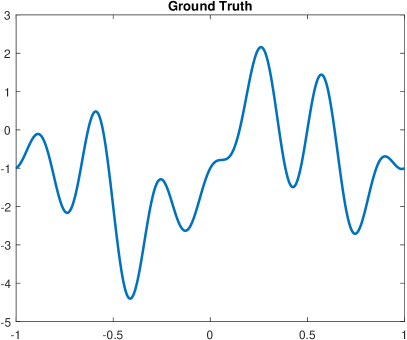
Figure 1: Ground truth $\dot{\rho}$

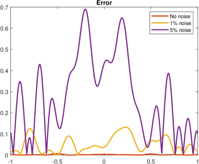
Figure 2: Left: Reconstructed $\dot{\rho}$ with $0\%,1\%,5\%$ Gaussian noise and the ground truth. Right: The corresponding error between the reconstruction result and the ground truth. The relative $L^{2}$-errors are $0.14\%,3.66\%$ and $19.37\%$, respectively.

Experiment 2. In this experiment, we consider a discontinuous perturbation

$$\dot{\rho}=\chi_{[-1,-\frac{1}{6}]}-\chi_{[-\frac{1}{6},\frac{1}{4}]},$$

where $\chi$ is the characteristic function. The Fourier series of $\dot{\rho}$ is given by

$$\dot{\rho}=\frac{5}{24}+\sum_{n=1}^{\infty}\left[-\frac{\sin\left(\frac{n\pi}{4}\right)+2\sin\left(\frac{n\pi}{6}\right)}{n\pi}\cos(n\pi x)+\frac{\cos(n\pi)+\cos\left(\frac{n\pi}{4}\right)+2\cos\left(\frac{n\pi}{6}\right)}{n\pi}\sin(n\pi x)\right].$$

With the choice of the basis functions (30), we can only expect to reconstruct the orthogonal projection:

$$\dot{\rho}_{N}\coloneqq\frac{5}{24}+\sum_{n=1}^{N}\left[-\frac{\sin\left(\frac{n\pi}{4}\right)+2\sin\left(\frac{n\pi}{6}\right)}{n\pi}\cos(n\pi x)+\frac{\cos(n\pi)+\cos\left(\frac{n\pi}{4}\right)+2\cos\left(\frac{n\pi}{6}\right)}{n\pi}\sin(n\pi x)\right],$$

see Figure 3. We plot the reconstruction result and the corresponding error with respect to the orthogonal projection $\dot{\rho}_{N}$ with different noise level in Figure 4.

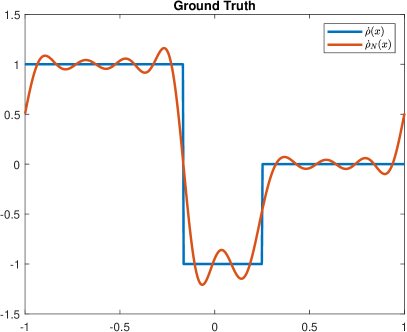
Figure 3: Ground truth $\dot{\rho}$

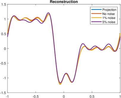
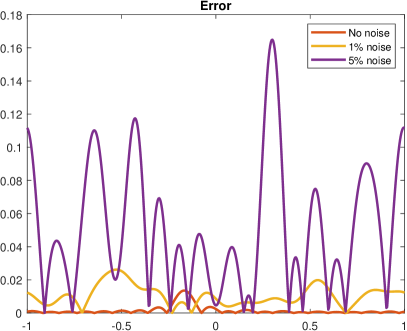
Figure 4: Left: Reconstructed $\dot{\rho}$ with $0\%,1\%,5\%$ Gaussian noise and the ground truth. Right: The corresponding error between the reconstruction result and the ground truth. The relative $L^{2}$-errors are $0.39\%,1.57\%$ and $8.15\%$, respectively.

Experiment 3. In this experiment, we apply the algorithm to the non-linear IBVP where

$$\rho=\rho_{0}+\varepsilon\dot{\rho}+\varepsilon^{2}\ddot{\rho},$$

with $\varepsilon=0.001$ and

$$\dot{\rho}=\sin(\pi x)+\sin(2\pi x)-\cos(5\pi x)+\cos(7\pi x)-1,\qquad\ddot{\rho}=200\sin(25\pi x).$$

See Figure 5 for the graph of $\rho$. Since

$$\Lambda_{\rho}-\Lambda_{\rho_{0}}\approx\varepsilon\dot{\Lambda}_{\dot{\rho}}=\dot{\Lambda}_{\varepsilon\dot{\rho}}$$

when $\varepsilon$ is small, we can use $\varepsilon^{-1}(\Lambda_{\rho}-\Lambda_{\rho_{0}})$ as an approximation of $\dot{\Lambda}_{\dot{\rho}}$ in (15). In this case, $\Lambda_{\rho}f$ and $\Lambda_{\rho_{0}}f$ are computed by numerically solving the forward problem (3) with $\rho$ and $\rho_{0}\equiv 1$. We then apply Algorithm 1 to find $\dot{\rho}$, and view $1+\dot{\rho}$ as an approximation of the ground truth $\rho$. In the experiment, we added the Gaussian noise to the difference $\Lambda_{\rho}-\Lambda_{\rho_{0}}$ rather than to $\Lambda_{\rho}f$ and $\Lambda_{\rho_{0}}f$ individually, see [30] for discussion of the difference. The reconstruction and the respective errors with $0\%,1\%,5\%$ Gaussian noise are illustrated in Figure 6.

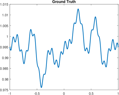
Figure 5: Ground truth $\rho$

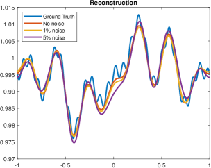
Figure 6: Left: Reconstructed $\rho$ with $0\%,1\%,5\%$ Gaussian noise and the ground truth. Right: The corresponding error between the reconstruction result and the ground truth. The relative $L^{2}$-errors are $18.09\%,20.95\%$ and $26.46\%$, respectively.

Appendix

We provide a rigorous proof to show that the operator $\dot{\Lambda}_{\dot{\rho}}$ derived in the introduction using the formal argument is indeed the Fréchet derivative of the nonlinear map $\rho\mapsto\Lambda_{\rho}$ at $\rho_{0}$ along $\dot{\rho}$.

Denote by $\mathcal{L}(X,Y)$ the Banach space of bounded linear operators from $X$ to $Y$. The IBVP (1) aims to invert the following nonlinear map

$$\mathcal{F}:\rho\in C^{\infty}(\overline{\Omega})\mapsto\Lambda_{\rho}\in\mathcal{L}(H^{\frac{5}{2}}((0,2T)\times\partial\Omega),H^{\frac{1}{2}}((0,2T)\times\partial\Omega))$$

Suppose $\rho=\rho_{0}+\dot{\rho}$ with $\rho_{0}\in C^{\infty}(\overline{\Omega})$ and $\dot{\rho}\in C_{c}^{\infty}(\Omega)$, define the following linear operator

$$\operatorname*{d\!}\mathcal{F}:\dot{\rho}\in C_{c}^{\infty}(\Omega)\mapsto\dot{\Lambda}_{\dot{\rho}}\in\mathcal{L}(H^{\frac{5}{2}}((0,2T)\times\partial\Omega),H^{\frac{1}{2}}((0,2T)\times\partial\Omega))$$

where $\dot{\Lambda}_{\dot{\rho}}$ is the linearized ND map defined in (5).

Proposition 15.

The nonlinear map $\mathcal{F}$ is Frechét differentiable at $\rho_{0}\in C^{\infty}(\overline{\Omega})$, and the Frechét derivative along the direction $\dot{\rho}\in C_{c}^{\infty}(\Omega)$ is $\dot{\Lambda}_{\dot{\rho}}$.

Proof.

In order to show that $\mathcal{F}$ is Frechét differentiable, we will show that

$$\|\mathcal{F}(\rho)-\mathcal{F}(\rho_{0})-\operatorname*{d\!}\mathcal{F}(\dot{\rho})\|_{\mathcal{L}(H^{\frac{5}{2}}((0,2T)\times\partial\Omega),H^{\frac{1}{2}}((0,2T)\times\partial\Omega))}=O(\|\dot{\rho}\|_{W^{1,\infty}(\Omega)}^{2})$$

as $\|\dot{\rho}\|_{W^{1,\infty}(\Omega)}\to 0$, which is equivalent to

$$\|\Lambda_{\rho}f-\Lambda_{\rho_{0}}f-\dot{\Lambda}_{\dot{\rho}}f\|_{H^{\frac{1}{2}}((0,2T)\times\partial\Omega)}=O(\|\dot{\rho}\|_{W^{1,\infty}(\Omega)}^{2}\|f\|_{H^{\frac{5}{2}}((0,2T)\times\partial\Omega)})$$

for any $f\in H^{\frac{5}{2}}((0,2T)\times\partial\Omega)$ as $\|\dot{\rho}\|_{W^{1,\infty}(\Omega)}\to 0$.

Write $u=u_{0}+\delta u$, where $u$ and $u_{0}$ are the solutions of (1) and (3), respectively. Then $\delta u$ satisfies the equation

$$\left\{\begin{aligned} \rho_{0}\delta u_{tt}-\Delta\delta u+q\delta u&=-\dot{\rho}\partial^{2}_{t}u\qquad\qquad&&\text{in }(0,2T)\times\Omega\\ \partial_{\nu}\delta u&=0&&\text{on }(0,2T)\times\partial\Omega\\ \delta u(0,x)=\delta u_{t}(0,x)&=0&&x\in\Omega\end{aligned}\right.$$

Using the regularity estimate for wave euation and the trace theorem, we have

$$\|\delta u\|_{H^{2}((0,2T)\times\Omega)}\leq C\|\dot{\rho}u_{tt}\|_{H^{1}((0,2T)\times\Omega)}\leq C\|u\|_{H^{3}((0,2T)\times\Omega)}\|\dot{\rho}\|_{W^{1,\infty}(\Omega)}$$

On the other hand, denote $w\coloneqq\delta u-\dot{u}$; it satisfies

$$\left\{\begin{aligned} \rho_{0}w_{tt}-\Delta w+qw&=-\dot{\rho}\partial^{2}_{t}\delta u\qquad\qquad&&\text{in }(0,2T)\times\Omega\\ \partial_{\nu}w&=0&&\text{on }(0,2T)\times\partial\Omega\\ w(0,x)=w_{t}(0,x)&=0&&x\in\Omega\end{aligned}\right.$$

Applying similar estimates yield

$$\|w\|_{H^{\frac{1}{2}}((0,2T)\times\partial\Omega)}\leq\|w\|_{H^{1}((0,2T)\times\Omega)}\leq C\|\dot{\rho}\delta u_{tt}\|_{L^{2}((0,2T)\times\Omega)}\leq C\|\delta u\|_{H^{2}((0,2T)\times\Omega)}\|\dot{\rho}\|_{W^{1,\infty}(\Omega)}.$$

Notice that $w|_{[0,2T]\times\partial\Omega}=\Lambda_{\rho}f-\Lambda_{\rho_{0}}f-\dot{\Lambda}_{\dot{\rho}}f$. These estimates combined give

$$\|\Lambda_{\rho}f-\Lambda_{\rho_{0}}f-\dot{\Lambda}_{\dot{\rho}}f\|_{H^{\frac{1}{2}}((0,2T)\times\partial\Omega)}\leq C\|u\|_{H^{3}((0,2T)\times\Omega)}\|\dot{\rho}\|^{2}_{W^{1,\infty}(\Omega)}.$$

Finally, the well-posedness estimate for the forward boundary value problem [13] gives

$$\|u\|_{H^{3}((0,2T)\times\Omega)}\leq C\|f\|_{H^{\frac{5}{2}}((0,2T)\times\partial\Omega)}.$$

This completes the proof. ∎

References

- [1] M. Belishev. On an approach to multidimensional inverse problems for the wave equation. In Soviet Math. Dokl, volume 36, pages 481–484, 1988.
- [2] M. Belishev and V. Y. Gotlib. Dynamical variant of the bc-method: theory and numerical testing. Journal of Inverse and Ill-Posed Problems, 7(3):221–240, 1999.
- [3] M. I. Belishev. Recent progress in the boundary control method. Inverse Problems, 23(5):R1–R67, 2007.
- [4] M. I. Belishev, I. B. Ivanov, I. V. Kubyshkin, and V. S. Semenov. Numerical testing in determination of sound speed from a part of boundary by the bc-method. Journal of Inverse and Ill-posed Problems, 24(2):159–180, 2016.
- [5] M. I. Belishev and Y. V. Kuryiev. To the reconstruction of a Riemannian manifold via its spectral data (bc–method). Communications in partial differential equations, 17(5-6):767–804, 1992.
- [6] K. Bingham, Y. Kurylev, M. Lassas, and S. Siltanen. Iterative time-reversal control for inverse problems. Inverse Problems & Imaging, 2(1):63, 2008.
- [7] A. Blagoveshchenskii. The inverse problem in the theory of seismic wave propagation. In Spectral Theory and Wave Processes, pages 55–67. Springer, 1967.
- [8] E. Blåsten, F. Zouari, M. Louati, and M. S. Ghidaoui. Blockage detection in networks: The area reconstruction method. arXiv preprint arXiv:1909.05497, 2019.
- [9] J. Cheng, V. Isakov, and S. Lu. Increasing stability in the inverse source problem with many frequencies. Journal of Differential Equations, 260(5):4786–4804, 2016.
- [10] M. V. De Hoop, P. Kepley, and L. Oksanen. An exact redatuming procedure for the inverse boundary value problem for the wave equation. SIAM Journal on Applied Mathematics, 78(1):171–192, 2018.
- [11] M. V. de Hoop, P. Kepley, and L. Oksanen. Recovery of a smooth metric via wave field and coordinate transformation reconstruction. SIAM Journal on Applied Mathematics, 78(4):1931–1953, 2018.
- [12] G. Eskin. Inverse hyperbolic problems with time-dependent coefficients. Communications in Partial Differential Equations, 32(11):1737–1758, 2007.
- [13] L. C. Evans. Partial differential equations and monge-kantorovich mass transfer. Current developments in mathematics, 1997(1):65–126, 1997.
- [14] L. C. Evans. Partial differential equations. Graduate studies in mathematics, 19(4):7, 1998.
- [15] T. Hrycak and V. Isakov. Increased stability in the continuation of solutions to the helmholtz equation. Inverse problems, 20(3):697, 2004.
- [16] V. Isakov. Increasing stability for the schrödinger potential from the dirichlet-to neumann map. Discrete and Continuous Dynamical Systems-S, 4(3):631–640, 2010.
- [17] V. Isakov, R.-Y. Lai, and J.-N. Wang. Increasing stability for the conductivity and attenuation coefficients. SIAM Journal on Mathematical Analysis, 48(1):569–594, 2016.
- [18] V. Isakov and S. Lu. Increasing stability in the inverse source problem with attenuation and many frequencies. SIAM Journal on Applied Mathematics, 78(1):1–18, 2018.
- [19] V. Isakov, S. Nagayasu, G. Uhlmann, and J.-N. Wang. Increasing stability of the inverse boundary value problem for the schrödinger equation. Contemp. Math, 615:131–141, 2014.
- [20] A. Katchalov, Y. Kurylev, and M. Lassas. Inverse boundary spectral problems, volume 123 of Chapman & Hall/CRC Monographs and Surveys in Pure and Applied Mathematics. Chapman & Hall/CRC, Boca Raton, FL, 2001.
- [21] J. Korpela, M. Lassas, and L. Oksanen. Discrete regularization and convergence of the inverse problem for 1+1 dimensional wave equation. Inverse Problems & Imaging, 13(3):575–596, 2019.
- [22] P.-Z. Kow, G. Uhlmann, and J.-N. Wang. Optimality of increasing stability for an inverse boundary value problem. SIAM Journal on Mathematical Analysis, 53(6):7062–7080, 2021.
- [23] Y. Kurylev. An inverse boundary problem for the Schrödinger operator with magnetic field. J. Math. Phys., 36(6):2761–2776, 1995.
- [24] Y. Kurylev and M. Lassas. Gelf’and inverse problem for a quadratic operator pencil. J. Funct. Anal., 176(2):247–263, 2000.
- [25] Y. Kurylev, L. Oksanen, and G. P. Paternain. Inverse problems for the connection Laplacian. J. Differential Geom., 110(3):457–494, 2018.
- [26] I. Lasiecka and R. Triggiani. Regularity theory of hyperbolic equations with non-homogeneous neumann boundary conditions. ii. general boundary data. Journal of Differential Equations, 94(1):112–164, 1991.
- [27] S. Liu and L. Oksanen. A lipschitz stable reconstruction formula for the inverse problem for the wave equation. Transactions of the American Mathematical Society, 368(1):319–335, 2016.
- [28] S. Nagayasu, G. Uhlmann, and J.-N. Wang. Increasing stability in an inverse problem for the acoustic equation. Inverse Problems, 29(2):025012, 2013.
- [29] L. Oksanen. Solving an inverse obstacle problem for the wave equation by using the boundary control method. Inverse Problems, 29(3):035004, 2013.
- [30] L. Oksanen, T. Yang, and Y. Yang. Linearized boundary control method for an acoustic inverse boundary value problem. Inverse Problems, 38(11):114001, 2022.
- [31] L. Pestov, V. Bolgova, and O. Kazarina. Numerical recovering of a density by the bc-method. Inverse Problems & Imaging, 4(4):703, 2010.
- [32] P. Stefanov and G. Uhlmann. Stability estimates for the hyperbolic Dirichlet to Neumann map in anisotropic media. journal of functional analysis, 154(2):330–358, 1998.
- [33] P. Stefanov and G. Uhlmann. Stable determination of generic simple metrics from the hyperbolic Dirichlet-to-Neumann map. International Mathematics Research Notices, 2005(17):1047–1061, 2005.
- [34] J. Sylvester and G. Uhlmann. A global uniqueness theorem for an inverse boundary value problem. Annals of mathematics, pages 153–169, 1987.
- [35] D. Tataru. Unique continuation for solutions to PDE’s; between Hormander’s theorem and Holmgren’s theorem. Communications in Partial Differential Equations, 20(5-6):855–884, 1995.
- [36] D. Tataru. Unique continuation for operatorswith partially analytic coefficients. Journal de mathématiques pures et appliquées, 78(5):505–521, 1999.
- [37] T. Yang and Y. Yang. A stable non-iterative reconstruction algorithm for the acoustic inverse boundary value problem. Inverse Problems & Imaging, 2021.