How Does Bayes Error Limit Probabilistic Robust Accuracy
Abstract
Adversarial examples pose a security threat to many critical systems built on neural networks. Given that deterministic robustness often comes with significantly reduced accuracy, probabilistic robustness (i.e., the probability of having the same label with a vicinity is ) has been proposed as a promising way of achieving robustness whilst maintaining accuracy. However, existing training methods for probabilistic robustness still experience non-trivial accuracy loss. It is unclear whether there is an upper bound on the accuracy when optimising towards probabilistic robustness, and whether there is a certain relationship between and this bound. This work studies these problems from a Bayes error perspective. We find that while Bayes uncertainty does affect probabilistic robustness, its impact is smaller than that on deterministic robustness. This reduced Bayes uncertainty allows a higher upper bound on probabilistic robust accuracy than that on deterministic robust accuracy. Further, we prove that with optimal probabilistic robustness, each probabilistically robust input is also deterministically robust in a smaller vicinity. We also show that voting within the vicinity always improves probabilistic robust accuracy and the upper bound of probabilistic robust accuracy monotonically increases as grows. Our empirical findings also align with our results.
1 Introduction
Neural networks (NNs) achieve remarkable success in various applications, including many security-critical systems [18, 37]. At the same time, several security vulnerabilities in NNs have been identified, including adversarial attacks that generate adversarial examples. Adversarial examples are inputs that are carefully crafted by adding human imperceptible perturbation to normal inputs to trigger wrong predictions [19]. Their presence is particularly concerning in security-critical NN applications.
To defend against adversarial examples, various methods for improving a model’s robustness have been proposed. Adversarial training works by training NNs with a mix of normal and adversarial examples, either pre-generated or generated during training. As it does not carry a formal guarantee on the achieved robustness [49], adversarially trained NNs are potentially vulnerable to new types of adversarial attacks [24, 43]. In contrast, certified training aims to provide a formal guarantee of robustness. A method in this category typically incorporates robustness verification techniques during training [47], i.e., they aim to find a valuation of network parameters such that the model is provably robust to the training samples and some definition of vicinity. However, they are often impractical for multiple reasons including the irreducible errors due to Bayes error (the unavoidable inaccuracy in collecting or labelling training samples) which limits the level of accuracy that is achievable [7, 52].
Recent studies propose that probabilistic robustness, i.e., the probability of having adversarial examples within a vicinity is no more than a certain tolerance level , could be sufficient for many practical applications [35, 22, 53]. Furthermore, it is shown to be achievable with a smaller accuracy drop (5% when ) and less computational cost compared to certified training methods [35]. Probabilistic robustness thus balances between achieving high degrees of security and maintaining accuracy. However, it remains unclear if Bayes errors also limit the achievable performance when optimising towards probabilistic robustness i.e., probabilistic robust accuracy. Further, if an upper limit does exist, how is such a limit correlated to the tolerance level ?
In this work, we aim to answer these questions. The Bayes error, in the context of statistics and machine learning, is a fundamental concept related to the inherent uncertainty in any classification system [15]. It represents the minimum error for any classifier on a given problem and is determined by the overlap in the probability distributions of different classes [10]. We remark that the relevance of Bayes error in simple classification tasks may occasionally be questioned given that many datasets, such as MNIST, provide a single, definite label for each input [20]. However, real-world data often lacks this clarity due to inevitable information loss, e.g., during image capture or compression. For instance, the CIFAR-10H dataset showcases that over a third of CIFAR-10 inputs can be re-annotated with uncertain labels by human annotators (CIFAR-10H) [32]. Thus, this uncertainty leads to Bayes errors, which fundamentally constrain not only vanilla accuracy [15] but also deterministic robust accuracy [52] and probabilistic robust accuracy (as what will be shown in this work).
We study the limit on the probabilistic robust accuracy resulting from Bayes error. We first derive an optimal decision rule that maximises probabilistic robust accuracy. Similar to the Bayes classifier [9], the optimal decision rule for probabilistic robustness is also a Maximum A Posteriori (MAP [3]) probability decision, except that the posterior is regarding the vicinity, not a single input. Then, we show that the error from this optimal decision rule regarding probabilistic robustness is lower bounded by the Bayes error for deterministic robustness, but within a much smaller vicinity. After that, a relationship is established between the upper bound of probabilistic robust accuracy and the upper bound of vanilla accuracy or deterministic robust accuracy. We further show that the bound monotonically increases as grows. Empirically, we show that our bounds are consistent with what is observed on those probabilistically robust neural networks trained on various distributions.
2 Preliminary and Problem Definition
This section first reviews the background of robustness in machine learning. Then, we recall the Bayes error for the deterministic robustness of classification. Finally, we define our research problem.
2.1 Robustness in Neural Network Classification
We put the context in a -class classification problem where a classifier learns to fit a joint distribution over input space and label space . Let denote prediction, and an error captures the difference between and . That is, vanilla accuracy is and thus its error is . The capital Upsilon with a plus sign denotes accuracy itself, while a minus sign denotes its corresponding error.
Robustness measures the change in prediction when a perturbation occurs on the input [41]. If the prediction changes when an input is perturbed, then this input is an adversarial example. Formally, an input is an adversarial example of an input-label pair if [13, 19], where is the vicinity at . We define robustness to be the probability of not observing an adversarial example [23], as defined in Equation 1.
| (1) |
Remark 2.1 (Vicinity).
-vicinity also has an equivalent distribution notation . Let denote its probability density function (PDF) such that means is in -vicinity. is an even and quasiconcave function e.g., the Gaussian function. Section A.1 shows the equivalence.
Deterministic Robustness Deterministic robustness requires a zero probability of adversarial examples occurring in a vicinity. It is difficult as achieving is challenging. Although adversarial training [13] empirically reduces adversarial examples [11], it lacks a formal guarantee. Meanwhile, certified training [28] guarantees deterministic robustness through integrating NN verification during training, often resulting in a significant accuracy drop (35%) [21].
Probabilistic Robustness While deterministic robustness is often infeasible without seriously compromising accuracy, probabilistic robustness claims to balance robustness and accuracy [35]. Probabilistic robustness is defined as in Equation 2, where a tolerance level limits the probability of having adversarial examples in a vicinity . Here, a small portion (such as 1% [53]-50% [8]) of adversarial examples within the vicinity is considered acceptable. Probabilistic robustness is often sufficient in practice [35]. Indeed, safety certification of many safety-critical domains such as aviation requires keeping safety violation probabilities below a non-zero threshold [14].
| (2) |
2.2 An Upper Bound of Deterministic Robustness from Bayes Error
The Bayes Error
In the presence of uncertainty in data distribution, a classifier (no matter how it is trained) inevitably makes some wrong predictions. Bayes error quantifies this inherent uncertainty and represents the irreducible error in accuracy [10, 12, 34], formally captured in Equation 3.
| (3) |
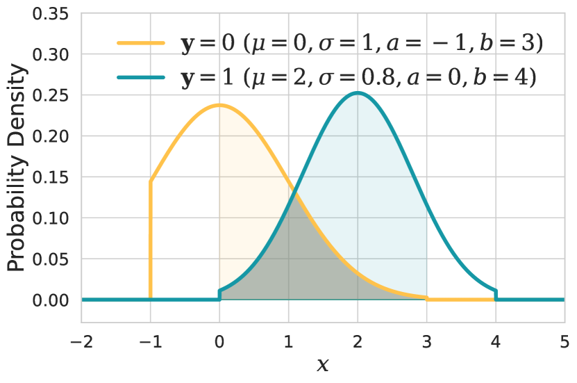
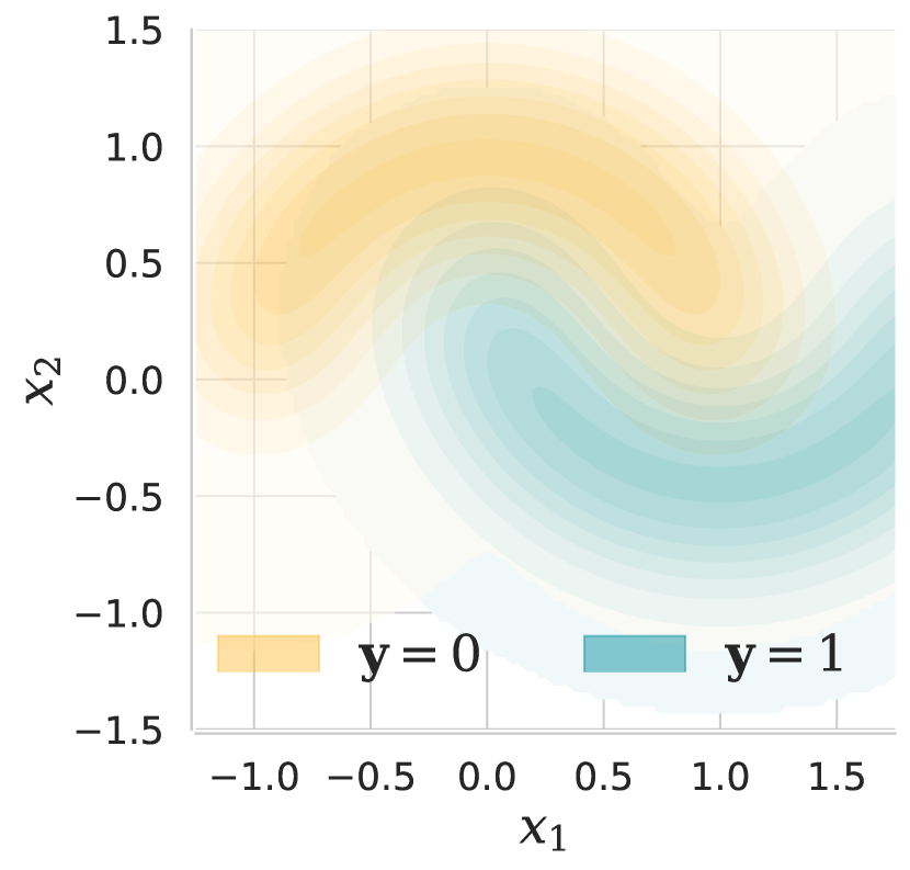
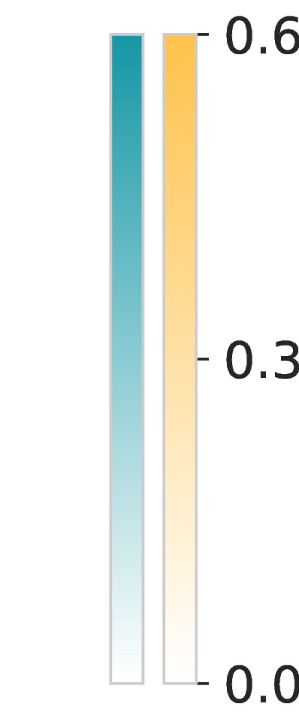
A classifier achieves the Bayes error when its predictions correspond to the class with maximal posterior probability. Such a classifier is known as a Bayes classifier. The posterior of other classes thus contributes to the irreducible error. An example illustrating the Bayes error is shown in Figure 1(a).
Bayes Error for Deterministic Robustness
Prior work [52] shows that optimising towards deterministic robustness makes the Bayes error worse. Besides the posterior of other classes, forcing a prediction to be consistent with its neighbours constitutes another source of Bayes error [52]. As in Equation 4, the Bayes error for deterministic robustness can be derived from the Bayes error of a convolved distribution . In , is convolved from vicinity and in .
| (4) |
where . where is the “hardened” distribution of , i.e., one-hot of Argmax posterior. represents a domain near the boundary where the marginal probability rather than joint probability contributes to the Bayes error for deterministic robustness. Therefore, the Bayes error for deterministic robustness of is the Bayes error of plus the joint probability of non-max classes in . As shown in [52], deterministic robustness has an upper bound of 1 minus this irreducible error. Figure 1(b) illustrates the Bayes error for deterministic robustness.
2.3 Problem Definition
The fundamental problem in this study is finding an upper bound of probabilistic robust accuracy. Further, we aim to establish a relation between this upper bound and the tolerance level, i.e., . Formally, we solve the minimisation problem in Equation 5 where .
| (5) |

3 Method
In the following, we study the upper bound of probabilistic robust accuracy. We first model the error when optimising towards probabilistic robustness and derive an optimal decision rule. Then, we study the Bayes error obtained from this rule. Further, we formally establish the relationship between the upper bounds of vanilla accuracy, probabilistic robust accuracy, and deterministic robust accuracy.
3.1 Error Modelling and Optimal Decision Rule for Probabilistic Robustness
To find Bayes error when optimising towards probabilistic robustness given distribution , we first model . Intuitively, an error happens if the prediction is wrong or many of the samples in the vicinity are predicted wrongly. We denote the error from the former case as incorrectness and the latter as inconsistency. We analyze each type of error and their combined effect.
Incorrectness
The incorrectness for any example is simply . The incorrectness of a prediction at an input given all possible labels considers posterior at , as in Equation 6. Incorrectness is minimum when equals the class with the highest posterior.
| (6) |
Inconsistency
Inconsistency results from prediction at being not the same as some of its neighbours. Let denote the probability of a neighbour of having a prediction different from . Since this probability is parameterised by , it can be reformulated as . Let and . Intuitively, is the probability of a neighbour predicted as class-. Thus, the probability of a neighbour of having a different prediction from can be written as Equation 7.
| (7) |
Inconsistency exists when . This thresholding can be represented by a unit step function () that takes an input . Thus, inconsistency at is expressed as Equation 8. Also, Lemma 3.1 suggests that takes value from .
| (8) |
Lemma 3.1.
For the prediction of input to be consistent, at most one class has a prediction probability in -vicinity. Thus, . (Proof is provided in Section B.1.)
The overall error across the distribution
Considering probabilistic robustness, the error at input is a combined error of and at . We need two intuitions to derive the combined error. First, if , the combined error is always 1. Second, if , the combined error equals . Note that takes value from and takes binary value from . The combined error is expressed as Equation 9 whose derivation is in Section B.2.
| (9) | ||||
Note that in general, the errors are functions of , and . For simplicity, when , , , or can be inferred from the context, we simply omit them, e.g., the simplest case is written as to denote the incorrectness, to denote inconsistency, and to denote the combined error.
To model the distribution-wise error of classifier on , we compute the expectation of across . Formally, , where is the marginal probability in . Hereby, we get , the error when optimising towards probabilistic robustness.
To minimise of any measurable classification function , we explore the optimal decision rules for probabilistic robustness. From Equation 9, we can establish a Maximum A Posteriori optimal decision rule, whose formal statement is given in Theorem 3.2.
Theorem 3.2.
If is optimal for the probabilistic robustness on a given distribution, i.e., , we would always have .
Proof.
Let and be two distinct classification functions such that and . If we can prove , then we can know must be optimal for probabilistic robustness. First, we denote and . Then,
| (10) |
Since , we get . Recall from Lemma 3.1, we get . Consequently, we have . Therefore, . This inequality applies to any input . Hence, a classification function like is optimal. An extended proof is in Section B.3. ∎
Intuitively, the theorem states that when optimising towards probabilistic robustness, a Bayes (optimal) classifier would always classify a sample with the most popular label in the vicinity.
3.2 Bayes Error for Probabilistic Robustness from Bayes Error for Deterministic Robustness
The Bayes classifier, regarding probabilistic robustness, is closely related to the most popular label in its vicinity, leading us to study the properties of . Intuitively, is the probability of a neighbour predicted as class-. Formally, has an equivalent convolutional form as
| (11) |
where denotes convolution and denotes an indicator function returning 1 if of input equals . is the probability density function of vicinity distribution, e.g., uniform distribution.
Intuitively, convolution acts as a smoothing operation. Thus, is expected to change gradually as moves in . Similarly, is unlikely to switch frequently. This implies that under the optimal probabilistic robustness condition, predictions do not change randomly or frequently (in ) but exhibit a form of continuity. Lemma 3.3 and Theorem 3.4 formally states this intuition. Specifically, Lemma 3.3 states that changes gradually as moves in . Moreover, Theorem 3.4 states that the Bayes classifier (for probabilistic robustness) achieves deterministic robustness with a much smaller vicinity at any input that achieves probabilistic robustness.
Lemma 3.3.
The change in resulting from shifting an input by a certain distance within the vicinity is bounded in any direction . Formally: where is the set of all unit vectors in ,
| (12) | |||
Proof of Lemma 3.3 is given in Section B.4. Essentially, for all inputs shifting a distance , the value difference between the original input and the shifted input will be bounded by the 1 minus the minimum overlap between two vicinities that are apart. From Equation 12, the correlation between the distance and maximum change of can be modelled as a function of expressed as
| (13) |
Note that is a monotonic function, i.e., a greater shift distance is required if the maximal change in needs to be increased. Theorem 3.4 leverages this monotonicity to formally show the connection between the Bayes error when optimising towards probabilistic robustness and that towards deterministic robustness.
Theorem 3.4.
If is optimal for the probabilistic robustness on a given distribution, i.e., , then there is a lower bound on the distance between an input and any of its adversarial examples if probabilistic consistency is satisfied on . Formally,
| (14) | |||
Proof.
Suppose an input whose prediction is consistent, i.e., . Let denote this predicted class. Let and denote two scalar distances to shift and assume the following features of these two distances. First, and . The latter indicates that in some direction, moving the input by a distance of results in a change in greater than . Second, . From the first condition, we can derive that
| (15) |
In other words, we can find some vector such that this shift results in a vicinity overlap smaller than the minimum vicinity overlap caused by a -magnitude shift.
Next, we further shift along direction but with the magnitude . This new position, , is farther away from than is because . Additionally, results in at most the same vicinity overlap (size) as does because is quasiconcave. Formally,
| (16) |
Observe that Equation 16 contradicts (15). Therefore, the two assumptions cannot hold simultaneously. An adversarial example requires . Thus, if , the distance between a consistent input and any of its adversarial examples is greater than (or equal to) . The rationale of is proven in Section B.5. ∎
Intuitively, at optimal probabilistic robust accuracy, if an input has a probabilistically consistent prediction, all its neighbours in some specific vicinity are predicted the same. Namely, the prediction at this input is deterministically robust within this (likely smaller) vicinity. Corollary 3.5 suggests that the bounds stated in Theorem 3.4 persist even as the shift approaches zero.
Corollary 3.5.
There exists a finite real value such that for all inputs, the directional derivative value with respect to any arbitrary nonzero vector (unit vector) does not exceed this finite value and does not fall below the negative of this value. Formally: where denotes the dot product,
| (17) |
Proof of Corollary 3.5 is provided in Section B.6. A one-dimensional example in Section B.7 illustrates this idea. We then present an implication of Theorem 3.4 for -norm in Corollary 3.6.
Corollary 3.6.
If is optimal for the probabilistic robustness with respect to an -vicinity on distribution , then the vicninty size of the deterministically robust vicinity around each probabilistically consistent input is .
Proof of Corollary 3.6 is in Section B.8. We visualise its effect using a two-dimensional example in Figure 1(d). Let be two probabilistically consistent inputs and . To minimise , must be in the diagonal direction (as in Corollary 3.6). The shift from to is . Each triangle accounts for of the original vicinity volume. Box has side length . Thus, solving , we get has vicinity size . Although Corollary 3.6 concerns , we can analyse other types similarly, i.e., find the direction with the fastest vicinity overlap decrease and measure the distance to the nearest adversarial example.
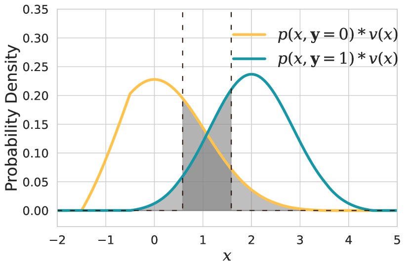
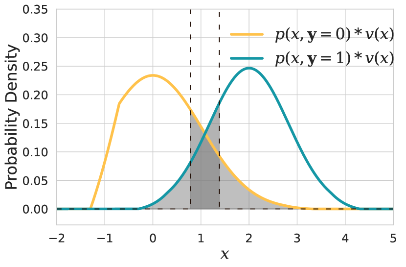
In brief, an optimal probabilistic robust accuracy has the following implications. Theorem 3.4 suggests that each probabilistically robust input is also deterministically robust, but within a much smaller vicinity. Corollary 3.6 further quantifies the size of this vicinity. Particularly, the order lets vicinity shrink fast as grows, making probabilistic robust accuracy higher. Overall, deterministic robust accuracy with the smaller vicinity bounds probabilistic robust accuracy. This is formally captured in Theorem 3.7. The effect of this reduced Bayes uncertainty is illustrated in Figure 1(c).
Theorem 3.7.
Given distribution , vicinity with size , and tolerance level , the probabilistic robust accuracy has an upper bound as shown in Equation 18, where or is the “smaller” vicinity and follows the definition in Equation 4, denoting the domain near the boundary.
| (18) | ||||
Proof.
Theorem 3.4 infers at optimal probabilistic robust accuracy. Consider this expression in the form of . This implies that the occurrence rate of Event 2 (deterministic robust accuracy with ) always upper bounds the rate of Event 1 (probabilistic robust accuracy with ). Additionally, the deterministic robust accuracy with has an upper bound, as what has been shown in [52]. ∎
Besides the upper bound, we also find a relatively loose lower bound of probabilistic robust accuracy as shown in Theorem 3.8. This lower bound is the deterministic robust accuracy when the vicinity size is the same as the vicinity size assumed for probabilistic robustness.
Theorem 3.8.
The upper bound of probabilistic robust accuracy monotonically increases as grows. Further, for all tolerance levels , the upper bound of probabilistic robust accuracy lies between the upper bound of deterministic robust accuracy and the upper bound of vanilla accuracy. Formally,
| (19) | ||||
Proof.
Let and , and then we get the sign of is the same as . This is because the posterior probability is non-negative. Since , and unit step function monotonically increases, we get . A smaller leads to a lower or equal upper bound of probabilistic robust accuracy. For deterministic robust accuracy, , which is the least value. Thus, deterministic robust accuracy has a smaller upper bound than probabilistic robust accuracy does.
On the other hand, from the intuition of error combination in Section 3.1, we get that the combined error is . As , we get . Note that the expectation of is the error in vanilla accuracy. Thus, . So it is with their upper bounds. We also provide an extended proof for this theorem in Section B.9. ∎
In summary, we show that probabilistic robust accuracy is both lower and upper bounded. We also show why the upper bound of probabilistic robust accuracy can be much greater than that of deterministic robust accuracy. Intuitively, our result suggests that probabilistic robustness indeed allows us to sacrifice much less accuracy, compared to that of deterministic robustness. Furthermore, adopting a larger (more relaxed) (up to 1/2) can effectively increase probabilistic robust accuracy.
4 Experiment
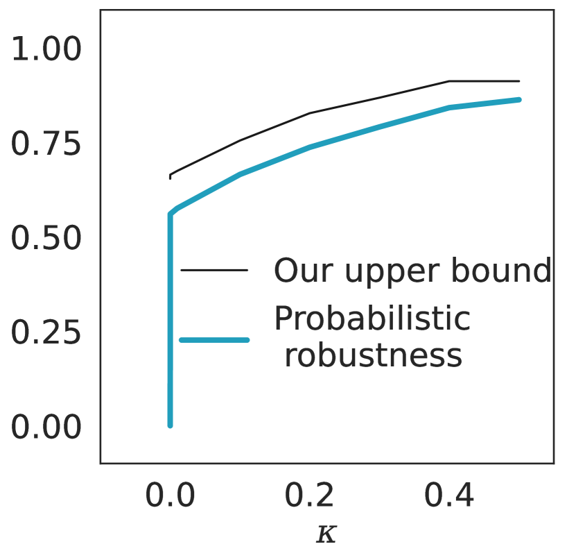
We conduct experiments111Available at https://github.com/soumission-anonyme/irreducible.git to validate the above established results empirically. Note that Theorem 3.2 infers voting is optimal. Section 3.2 establishes the probabilistic robust accuracy upper bound. Do these match empirical results? Further, ablation experiments on real-world distribution study how this upper bound changes as grows. The relationship between accuracy, probabilistic, and deterministic robust accuracy is also studied. In the following, we describe the setups and then answer these questions.
Setup
Our setup follows prior Bayes error studies [15, 52]. We include four datasets: Moons [31], Chan [6], FashionMNIST [46], and CIFAR-10 [17]. Given each dataset, we apply a direct method [15] to compute the Bayes error. -vicinity is set with for defining robustness on respective distribution. For deterministic robustness, the Bayes error follows Equation 4 [52]. For probabilistic robustness, we set by default [35] and vary only for the ablation study. More details are in Section C.1. Statistic significance is included in Section C.2.
Does voting always increase probabilistic robust accuracy empirically?
We first compute the probabilistic robust accuracy of some classifier . We then compute that of a voting classifier , where , with sample size 100. They are compared in Table 1. Training algorithms of include data augmentation (DA [39]), randomised smoothing (RS [8]), and condition value-at-risk (CVaR [35]) which is state-of-the-art (SOTA) for probabilistic robust accuracy. Note that voting always improves probabilistic robust accuracy (at least by +0.1% or on average +1.58% ). On DA and RS, the increase is significant (avg + 1.95%), partly because they are not designed specifically for probabilistic robustness. On CVaR, while modest (avg + 0.85%), we do observe an increase. This trend is maintained with a larger voting sample size (Section C.3).

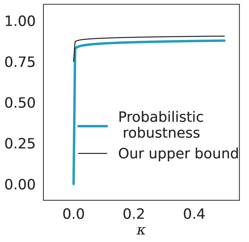
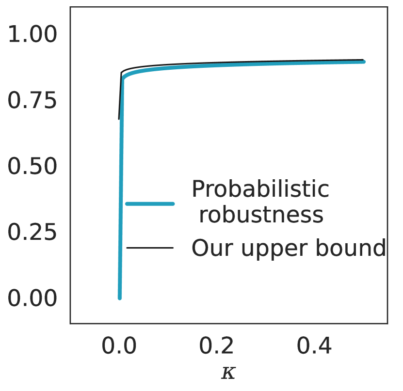
Is our upper bound empirically valid on existing neural networks?
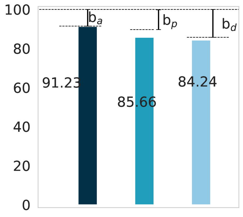
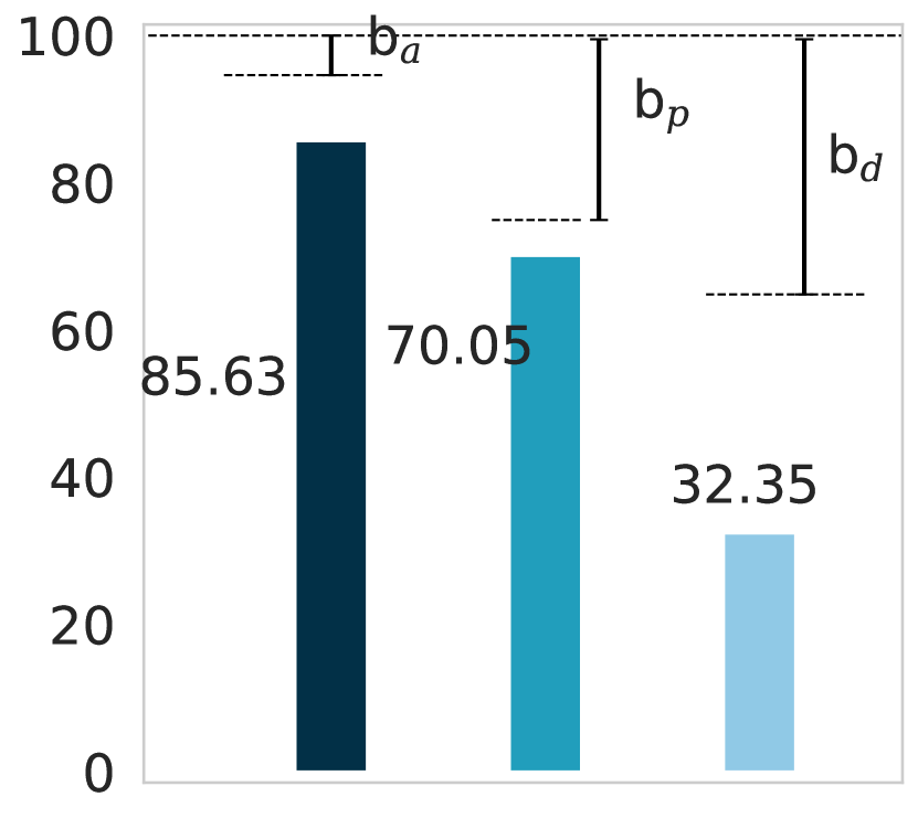
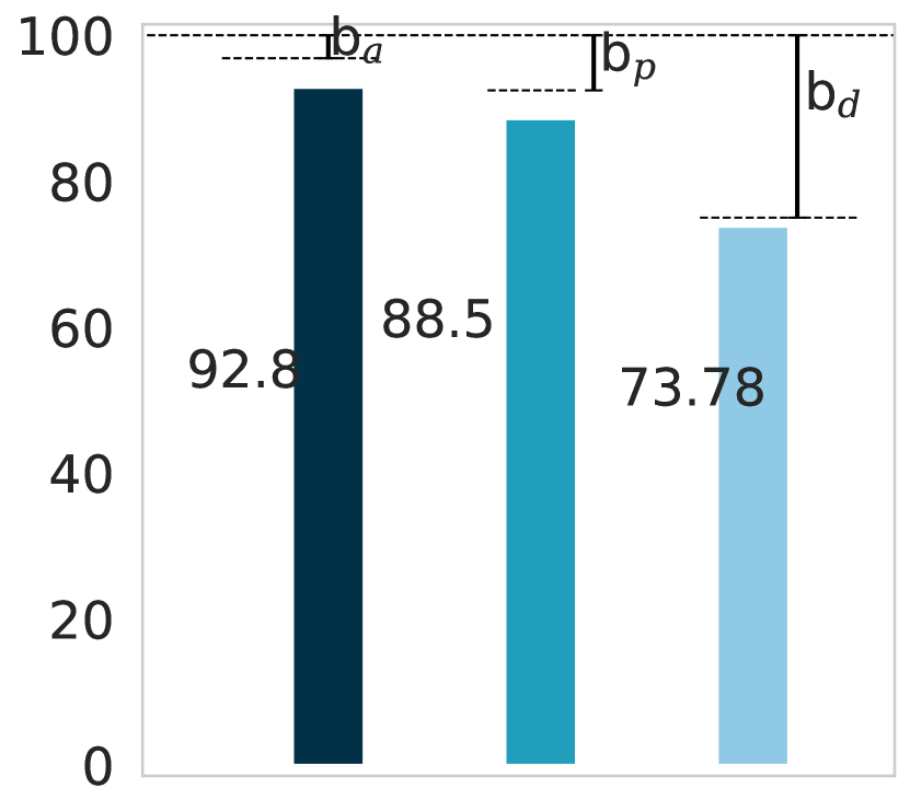
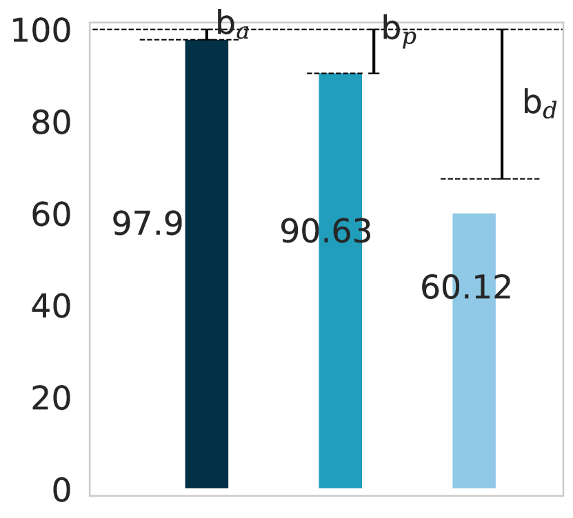
To check if indeed all trained classifiers respect the theoretical upper bound of probabilistic robust accuracy on any distribution, we compare the SOTA CVaR training and the bound. The middle column of each plot in Figure 2 demonstrates this comparison. We observe that the SOTA probabilistic robust accuracy never exceeds our theoretical bound. Intriguingly, on certain distributions like CIFAR-10, SOTA training almost meets its upper bound with a small gap (0.2%), while on others, a gap remains (on average 4.06%). Theoretically, a negative gap may also occur when a classifier overfits the data samples [15]. Our upper bound is empirically useful in approximating the room for improvement.
How does probabilistic robust accuracy compare to vanilla accuracy and deterministic robust accuracy in terms of upper bounds?
We observe in Figure 2 that invariably, the upper bound of probabilistic robust accuracy is lower than that of vanilla accuracy and higher than that of deterministic robust accuracy. In high-dimensional distributions, the upper bound of probabilistic robust accuracy is close to that of vanilla accuracy but over 27% higher than that of deterministic robust accuracy. This could be a result of the curse of dimensionality and much-reduced vicinity size according to Corollary 3.6. On Chan, the upper bound of probabilistic robustness is close to that of deterministic robust accuracy but over 20% lower than that of vanilla accuracy. This could be due to the high-frequency features in the distribution [52]. On Moons, these three bounds are close (at most 7% difference). The reason could be that this distribution is relatively smooth.
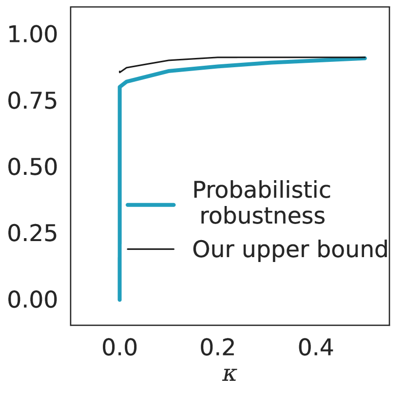
What is the effect of on the upper bound of probabilistic robust accuracy?
Given different , the upper bound of probabilistic robust accuracy can be different. We vary in increasing each time by 0.01. Figure 3 shows that this upper bound monotonically grows as grows, which matches Theorem 3.8. Besides, the growth is fast when is small (slope at ), and the growth rate decreases as grows (slope at ). Especially, for high-dimensional distributions, a small change in when is small, e.g. can significantly increase the upper bound. This could be explained by the order in Corollary 3.6. This is encouraging as it shows that by sacrificing deterministic robustness only slightly, we can already improve the accuracy significantly.
5 Related Work
This work is closely related to studies on Bayes errors and probabilistic robustness. Computing the Bayes error of a given distribution has been studied for over half a century [9], and one interesting topic is to derive or empirically estimate the upper and lower bounds of the Bayes error. Various -divergences, such as the Bhattacharyya distance [10] or the Henze-Penrose divergence [4, 36], have been studied. Other approaches include directly estimating the Bayes error with -divergence representation instead of using a bound [30], computing the Bayes error of generative models learned using normalizing flows [16, 42], or evaluate the Bayes error from data sample reassessment [15]. Recent studies apply Bayes error estimation to deterministic robustness beyond a vanilla accuracy perspective [52]. Our study extends this line of research and focuses on probabilistic robustness.
Improving robustness is a core topic in the recent decade [51, 44]. Adversarial training considers adversarial examples in the training phase [26, 13, 48, 45]. However, adversarially trained models do not come with a theoretical guarantee [50, 40, 2]. Certified training provides this guarantee by optimising bounds from formal verification during training but compromises performance on clean inputs [38, 28]. To mitigate these problems, probabilistic robustness methods such as PRoA [53] or CVaR [35] are proposed. Probabilistic robustness offers a desirable balance between robustness and accuracy, making it more applicable in real-world scenarios.
6 Conclusion
We investigate probabilistic robustness by formally deriving its upper bound. We find that the optimal prediction should be the Maximum A Posteriori of predictions in the vicinity. Then, we show that any probabilistically robust input is also deterministically robust within a smaller vicinity. Thus, the upper bound of probabilistic robust accuracy can be obtained from that of deterministic robust accuracy. We verify the empirical impact of this upper bound by comparing it with SOTA training and the upper bounds of vanilla accuracy or deterministic robust accuracy. Experiments match our theorems and show that our bounds could indicate room for improvement in practice.
Limitation
A limitation of our upper bound is that Theorem 3.4 requires the posterior probability to calculate the probabilistic robust accuracy upper bound whereas it might be difficult to obtain the posterior for some cases. This generally occurs for Bayes uncertainty analyses [9] in finding bounds of accuracy [42, 29, 27] or deterministic robustness [52]. Yet, this can be compensated by various density estimation methods [33, 52] or reevaluating the probability from a dataset [15].
References
- [1] Anish Athalye, Logan Engstrom, Andrew Ilyas, and Kevin Kwok. Synthesizing robust adversarial examples. In Jennifer Dy and Andreas Krause, editors, Proceedings of the 35th International Conference on Machine Learning, volume 80 of Proceedings of Machine Learning Research, pages 284–293. PMLR, 10–15 Jul 2018.
- [2] Mislav Balunovic and Martin T. Vechev. Adversarial training and provable defenses: Bridging the gap. In 8th International Conference on Learning Representations, ICLR 2020, Addis Ababa, Ethiopia, April 26-30, 2020. OpenReview.net, 2020.
- [3] Robert Bassett and Julio Deride. Maximum a posteriori estimators as a limit of bayes estimators. Mathematical Programming, 174(1):129–144, Mar 2019.
- [4] Visar Berisha, Alan Wisler, Alfred O. Hero, and Andreas Spanias. Empirically estimable classification bounds based on a nonparametric divergence measure. IEEE Transactions on Signal Processing, 64(3):580–591, 2016.
- [5] Saswati Bhattacharya and Mousumi Gupta. A survey on: Facial emotion recognition invariant to pose, illumination and age. In 2019 Second International Conference on Advanced Computational and Communication Paradigms (ICACCP), pages 1–6. IEEE, 2019.
- [6] Qingqiang Chen, Fuyuan Cao, Ying Xing, and Jiye Liang. Evaluating classification model against bayes error rate. IEEE Transactions on Pattern Analysis and Machine Intelligence, 45(8):9639–9653, 2023.
- [7] Ping-yeh Chiang, Renkun Ni, Ahmed Abdelkader, Chen Zhu, Christoph Studer, and Tom Goldstein. Certified defenses for adversarial patches. In 8th International Conference on Learning Representations, ICLR 2020, Addis Ababa, Ethiopia, April 26-30, 2020. OpenReview.net, 2020.
- [8] Jeremy Cohen, Elan Rosenfeld, and Zico Kolter. Certified adversarial robustness via randomized smoothing. In Kamalika Chaudhuri and Ruslan Salakhutdinov, editors, Proceedings of the 36th International Conference on Machine Learning, volume 97 of Proceedings of Machine Learning Research, pages 1310–1320. PMLR, PMLR, 09–15 Jun 2019.
- [9] K. Fukunaga and L. Hostetler. k-nearest-neighbor bayes-risk estimation. IEEE Transactions on Information Theory, 21(3):285–293, 1975.
- [10] Keinosuke Fukunaga. Introduction to Statistical Pattern Recognition (2nd Ed.). Academic Press Professional, Inc., USA, 1990.
- [11] Yaroslav Ganin, Evgeniya Ustinova, Hana Ajakan, Pascal Germain, Hugo Larochelle, François Laviolette, Mario March, and Victor Lempitsky. Domain-adversarial training of neural networks. Journal of Machine Learning Research, 17(59):1–35, 2016.
- [12] F.D. Garber and A. Djouadi. Bounds on the bayes classification error based on pairwise risk functions. IEEE Transactions on Pattern Analysis and Machine Intelligence, 10(2):281–288, 1988.
- [13] Ian J. Goodfellow, Jonathon Shlens, and Christian Szegedy. Explaining and harnessing adversarial examples. In Yoshua Bengio and Yann LeCun, editors, 3rd International Conference on Learning Representations, ICLR 2015, San Diego, CA, USA, May 7-9, 2015, Conference Track Proceedings, 2015.
- [14] Joris Guerin, Kevin Delmas, and Jérémie Guiochet. Certifying emergency landing for safe urban uav. In 2021 51st Annual IEEE/IFIP International Conference on Dependable Systems and Networks Workshops (DSN-W), pages 55–62, 2021.
- [15] Takashi Ishida, Ikko Yamane, Nontawat Charoenphakdee, Gang Niu, and Masashi Sugiyama. Is the performance of my deep network too good to be true? a direct approach to estimating the bayes error in binary classification. In The Eleventh International Conference on Learning Representations, 2023.
- [16] Durk P Kingma and Prafulla Dhariwal. Glow: Generative flow with invertible 1x1 convolutions. In S. Bengio, H. Wallach, H. Larochelle, K. Grauman, N. Cesa-Bianchi, and R. Garnett, editors, Advances in Neural Information Processing Systems, volume 31. Curran Associates, Inc., 2018.
- [17] Alex Krizhevsky, Geoffrey Hinton, et al. Learning multiple layers of features from tiny images. 2009.
- [18] Alexey Kurakin, Ian J. Goodfellow, and Samy Bengio. Adversarial examples in the physical world. In 5th International Conference on Learning Representations, ICLR 2017, Toulon, France, April 24-26, 2017, Workshop Track Proceedings. OpenReview.net, 2017.
- [19] Alexey Kurakin, Ian J. Goodfellow, and Samy Bengio. Adversarial machine learning at scale. In 5th International Conference on Learning Representations, ICLR 2017, Toulon, France, April 24-26, 2017, Conference Track Proceedings. OpenReview.net, 2017.
- [20] Yann LeCun, Corinna Cortes, and Chris Burges.
- [21] Linyi Li, Tao Xie, and Bo Li. Sok: Certified robustness for deep neural networks. In 44th IEEE Symposium on Security and Privacy, SP 2023, San Francisco, CA, USA, 22-26 May 2023. IEEE, 2023.
- [22] Renjue Li, Pengfei Yang, Cheng-Chao Huang, Youcheng Sun, Bai Xue, and Lijun Zhang. Towards practical robustness analysis for dnns based on pac-model learning. In Proceedings of the 44th International Conference on Software Engineering, ICSE ’22, page 2189–2201, New York, NY, USA, 2022. Association for Computing Machinery.
- [23] Wang Lin, Zhengfeng Yang, Xin Chen, Qingye Zhao, Xiangkun Li, Zhiming Liu, and Jifeng He. Robustness verification of classification deep neural networks via linear programming. In Proceedings of the IEEE/CVF Conference on Computer Vision and Pattern Recognition (CVPR), pages 11418–11427, June 2019.
- [24] Hao Liu, Xiangyu Zhu, Zhen Lei, and Stan Z. Li. Adaptiveface: Adaptive margin and sampling for face recognition. In Proceedings of the IEEE/CVF Conference on Computer Vision and Pattern Recognition (CVPR), June 2019.
- [25] Xingjun Ma, Bo Li, Yisen Wang, Sarah M. Erfani, Sudanthi N. R. Wijewickrema, Grant Schoenebeck, Dawn Song, Michael E. Houle, and James Bailey. Characterizing adversarial subspaces using local intrinsic dimensionality. In 6th International Conference on Learning Representations, ICLR 2018, Vancouver, BC, Canada, April 30 - May 3, 2018, Conference Track Proceedings. OpenReview.net, 2018.
- [26] Aleksander Madry, Aleksandar Makelov, Ludwig Schmidt, Dimitris Tsipras, and Adrian Vladu. Towards deep learning models resistant to adversarial attacks. In 6th International Conference on Learning Representations, ICLR 2018, Vancouver, BC, Canada, April 30 - May 3, 2018, Conference Track Proceedings. OpenReview.net, 2018.
- [27] Kevin R. Moon, Alfred O. Hero, and B. Véronique Delouille. Meta learning of bounds on the bayes classifier error. In 2015 IEEE Signal Processing and Signal Processing Education Workshop (SP/SPE), pages 13–18, 2015.
- [28] Mark Niklas Müller, Franziska Eckert, Marc Fischer, and Martin T. Vechev. Certified training: Small boxes are all you need. CoRR, abs/2210.04871, 2022.
- [29] Frank Nielsen. Generalized bhattacharyya and chernoff upper bounds on bayes error using quasi-arithmetic means. Pattern Recognition Letters, 42:25–34, 2014.
- [30] Morteza Noshad, Li Xu, and Alfred Hero. Learning to benchmark: Determining best achievable misclassification error from training data. arXiv preprint arXiv:1909.07192, 2019.
- [31] F. Pedregosa, G. Varoquaux, A. Gramfort, V. Michel, B. Thirion, O. Grisel, M. Blondel, P. Prettenhofer, R. Weiss, V. Dubourg, J. Vanderplas, A. Passos, D. Cournapeau, M. Brucher, M. Perrot, and E. Duchesnay. Scikit-learn: Machine learning in Python. Journal of Machine Learning Research, 12:2825–2830, 2011.
- [32] Joshua C. Peterson, Ruairidh M. Battleday, Thomas L. Griffiths, and Olga Russakovsky. Human uncertainty makes classification more robust. In Proceedings of the IEEE/CVF International Conference on Computer Vision (ICCV), October 2019.
- [33] Cédric Renggli, Luka Rimanic, Nora Hollenstein, and Ce Zhang. Evaluating bayes error estimators on real-world datasets with feebee. In Joaquin Vanschoren and Sai-Kit Yeung, editors, Proceedings of the Neural Information Processing Systems Track on Datasets and Benchmarks 1, NeurIPS Datasets and Benchmarks 2021, December 2021, virtual, 2021.
- [34] Brian D. Ripley. Pattern Recognition and Neural Networks. Cambridge University Press, 1996.
- [35] Alexander Robey, Luiz Chamon, George J. Pappas, and Hamed Hassani. Probabilistically robust learning: Balancing average and worst-case performance. In Kamalika Chaudhuri, Stefanie Jegelka, Le Song, Csaba Szepesvari, Gang Niu, and Sivan Sabato, editors, Proceedings of the 39th International Conference on Machine Learning, volume 162 of Proceedings of Machine Learning Research, pages 18667–18686. PMLR, 17–23 Jul 2022.
- [36] Salimeh Yasaei Sekeh, Brandon Oselio, and Alfred O. Hero. Learning to bound the multi-class bayes error. IEEE Transactions on Signal Processing, 68:3793–3807, 2020.
- [37] Mahmood Sharif, Sruti Bhagavatula, Lujo Bauer, and Michael K. Reiter. Accessorize to a crime: Real and stealthy attacks on state-of-the-art face recognition. In Proceedings of the 2016 ACM SIGSAC Conference on Computer and Communications Security, CCS ’16, pages 1528–1540, New York, NY, USA, 2016. Association for Computing Machinery.
- [38] Zhouxing Shi, Yihan Wang, Huan Zhang, Jinfeng Yi, and Cho-Jui Hsieh. Fast certified robust training with short warmup. In M. Ranzato, A. Beygelzimer, Y. Dauphin, P.S. Liang, and J. Wortman Vaughan, editors, Advances in Neural Information Processing Systems, volume 34, pages 18335–18349. Curran Associates, Inc., 2021.
- [39] Connor Shorten and Taghi M. Khoshgoftaar. A survey on image data augmentation for deep learning. Journal of Big Data, 6(1):60, Jul 2019.
- [40] Gagandeep Singh, Timon Gehr, Markus Püschel, and Martin Vechev. An abstract domain for certifying neural networks. Proc. ACM Program. Lang., 3(POPL), jan 2019.
- [41] Christian Szegedy, Wojciech Zaremba, Ilya Sutskever, Joan Bruna, Dumitru Erhan, Ian J. Goodfellow, and Rob Fergus. Intriguing properties of neural networks. In Yoshua Bengio and Yann LeCun, editors, 2nd International Conference on Learning Representations, ICLR 2014, Banff, AB, Canada, April 14-16, 2014, Conference Track Proceedings, 2014.
- [42] Ryan Theisen, Huan Wang, Lav R Varshney, Caiming Xiong, and Richard Socher. Evaluating state-of-the-art classification models against bayes optimality. In M. Ranzato, A. Beygelzimer, Y. Dauphin, P.S. Liang, and J. Wortman Vaughan, editors, Advances in Neural Information Processing Systems, volume 34, pages 9367–9377. Curran Associates, Inc., 2021.
- [43] Florian Tramer, Nicholas Carlini, Wieland Brendel, and Aleksander Madry. On adaptive attacks to adversarial example defenses. In H. Larochelle, M. Ranzato, R. Hadsell, M.F. Balcan, and H. Lin, editors, Advances in Neural Information Processing Systems, volume 33, pages 1633–1645. Curran Associates, Inc., 2020.
- [44] Jingyi Wang, Jialuo Chen, Youcheng Sun, Xingjun Ma, Dongxia Wang, Jun Sun, and Peng Cheng. Robot: Robustness-oriented testing for deep learning systems. In 2021 IEEE/ACM 43rd International Conference on Software Engineering (ICSE), pages 300–311, 2021.
- [45] Yisen Wang, Difan Zou, Jinfeng Yi, James Bailey, Xingjun Ma, and Quanquan Gu. Improving adversarial robustness requires revisiting misclassified examples. In 8th International Conference on Learning Representations, ICLR 2020, Addis Ababa, Ethiopia, April 26-30, 2020. OpenReview.net, 2020.
- [46] Han Xiao, Kashif Rasul, and Roland Vollgraf. Fashion-mnist: a novel image dataset for benchmarking machine learning algorithms. CoRR, abs/1708.07747, 2017.
- [47] Kaidi Xu, Zhouxing Shi, Huan Zhang, Yihan Wang, Kai-Wei Chang, Minlie Huang, Bhavya Kailkhura, Xue Lin, and Cho-Jui Hsieh. Automatic perturbation analysis for scalable certified robustness and beyond. In H. Larochelle, M. Ranzato, R. Hadsell, M.F. Balcan, and H. Lin, editors, Advances in Neural Information Processing Systems, volume 33, pages 1129–1141. Curran Associates, Inc., 2020.
- [48] Hongyang Zhang, Yaodong Yu, Jiantao Jiao, Eric Xing, Laurent El Ghaoui, and Michael Jordan. Theoretically principled trade-off between robustness and accuracy. In Kamalika Chaudhuri and Ruslan Salakhutdinov, editors, Proceedings of the 36th International Conference on Machine Learning, volume 97 of Proceedings of Machine Learning Research, pages 7472–7482. PMLR, 09–15 Jun 2019.
- [49] Huan Zhang, Hongge Chen, Zhao Song, Duane S. Boning, Inderjit S. Dhillon, and Cho-Jui Hsieh. The limitations of adversarial training and the blind-spot attack. In 7th International Conference on Learning Representations, ICLR 2019, New Orleans, LA, USA, May 6-9, 2019. OpenReview.net, 2019.
- [50] Huan Zhang, Tsui-Wei Weng, Pin-Yu Chen, Cho-Jui Hsieh, and Luca Daniel. Efficient neural network robustness certification with general activation functions. In Proceedings of the 32nd International Conference on Neural Information Processing Systems, volume 31 of NIPS’18, page 4944–4953, Red Hook, NY, USA, 2018. Curran Associates Inc.
- [51] Quan Zhang, Yongqiang Tian, Yifeng Ding, Shanshan Li, Chengnian Sun, Yu Jiang, and Jiaguang Sun. Coophance: Cooperative enhancement for robustness of deep learning systems. In Proceedings of the 32nd ACM SIGSOFT International Symposium on Software Testing and Analysis, ISSTA 2023, page 753–765, New York, NY, USA, 2023. Association for Computing Machinery.
- [52] Ruihan Zhang and Jun Sun. Certified robust accuracy of neural networks are bounded due to bayes errors. In Computer Aided Verification. Springer International Publishing, 2024.
- [53] Tianle Zhang, Wenjie Ruan, and Jonathan E. Fieldsend. Proa: A probabilistic robustness assessment against functional perturbations. In Massih-Reza Amini, Stéphane Canu, Asja Fischer, Tias Guns, Petra Kralj Novak, and Grigorios Tsoumakas, editors, Machine Learning and Knowledge Discovery in Databases, pages 154–170, Cham, 2023. Springer Nature Switzerland.
Appendix A Notations
A.1 Vicinity Notations
Definition A.1 (Vicinity).
Inputs within the vicinity of an input are imperceptible from . We call this vicinity an -vicinity. To capture imperceptibility, an -vicinity can be denoted in (at least four) different but equivalent notations, i.e., distance-threshold, set, distribution, and function notations. Occasionally, an input within -vicinity is called a neighbour of .
Distance-threshold Notation of Vicinity
The distance-threshold notation is one of the earliest notations to depict vicinity [25, 1, 5]. Here, the neighbour of a sample refers to an input that lies within a certain threshold distance from . Formally, is within -vicinity if and only if
| (20) |
where measures the distance between two inputs, and this distance needs to be smaller than a threshold to be considered imperceptible.
Specifically, the distance function can be defined in a variety of ways e.g., norm ( or ) or domain-specific transformations that preserve labels, such as tilting or zooming.
| (21) | ||||
where the transformation function can be, for example, an image rotation with a parameter determining the degree of rotation.
Set Notation of Vicinity
Here, the vicinity of a sample refers to a set containing all neighbours of . Given an input, all inputs whose distance to the given input is within a certain threshold form a set, defined as a vicinity of the given input. For any , its vicinity is expressed as
| (22) |
Since the corresponding distance function can be a representation of different distance measures, the set notation can also be a representation of various sets, i.e., could be -vicinities defined in two different ways.
Function Notation of Vicinity
The set or distance representation may be inconvenient sometimes [52]. We may sometimes need the notion of to quantify if is a neighbour of . For instance, if we would like to sum the marginal probability of all neighbours of , we can instead of to avoid a varying interval of integration.
In this case, a vicinity function, which is an equivalent form of the set, can be defined as
| (23) |
Essentially, Equation 23 can be viewed as a probability density function (PDF) uniformly defined over the vicinity around an input . Now we shift the x-coordinate by , we get
| (24) |
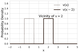
Assuming that the vicinity function is translation invariant, we can drop the subscript , and use a positive constant to represent , i.e., the volume of the vicinity. Thus, the vicinity function can be expressed as
| (25) |
An example of a one-dimensional input’s vicinity is shown in Figure 4.
Distribution Notation of Vicinity
When we need to sample from the vicinity, we need its distribution notation. The distribution notation for -vicinity is whose PDF is denoted as . If , we say is within -vicinity.
An imperceptible perturbation from any to means that is a ‘neighbour’ of , or equivalently, is in the -vicinity. -vicinity is a (probabilistic) distribution centred at . A standard vicinity is centred at the origin and its PDF is denoted as . Thus, the PDF centred any specific would be .
is typically an even and quasiconcave function. Formally,
| (26) | ||||
A uniform -vicinity assumes that all inputs outside an -norm of are distinguishable from and all inputs within this norm are equally imperceptible from . This vicinity function is captured in Equation 27 where parameter specifies a size.
| (27) |
The fraction in Equation 27 represents the inverse of the -norm volume, where denotes the gamma function. Vicinity functions assess the likelihood of being a neighbour to . In the uniform -norm context, all inputs within the norm are equally valid as neighbours and no inputs outside the norm are neighbours.
Remark A.2.
Adversarial examples of an input always reside -vicinity.
Appendix B Complete Proofs and Derivations
This section provides detailed proofs for various lemmas, theorems, or corollaries. For each, we restate the original claim followed by a more comprehensive proof than what appears in the main text. Additionally, we include detailed derivations for certain equations not covered in the theorems.
B.1 Proof of Lemma 3.1
Lemma 3.1.
For the predictions within the vicinity (of an input ) to be consistent, at most one class has a prediction probability exceeding in this vicinity. Thus, .
Proof.
Assume that such that any that is greater than or equal to satisfies the consistency condition because . Hence, there may exist some such that and
| (28) |
The existence of such distinct indices implies that if prediction at is , it is consistent with its neighbours. Similarly, if prediction at is , it is consistent with its neighbours. However, since , it is not possible for the neighbours’ predictions to simultaneously be consistent with both and . This scenario contradicts Equation 28, and thus the initial assumption does not hold. ∎
B.2 Derivation of the Combined Error Considering probabilistic robustness
Considering probabilistic robustness, the error at input is a combined error of and at . As discussed, we use two intuitions to derive the combined error. First, if , the combined error is always 1. Second, if , the combined error equals . Note that inconsistency is a binary value that takes either 0 or 1 while incorrectness takes a real value from 0 to 1 depending on the posterior at input. In the following, we derive the combined error as expressed in Equation 9.
| (29) | ||||
B.3 Extended Proof of Theorem 3.2
Theorem 3.2.
If is optimal for the probabilistic robustness on a given distribution, i.e., , we would always have .
Proof.
Let and be two distinct classification functions such that and . We want to prove , such that must be optimal for probabilistic robustness. First, we denote . Then,
| (30) | ||||
Since , we get . Recall from Lemma 3.1, we get
| (31) |
Consequently, when the input of a unit step function is negative, we have . Therefore, we get the following expression where the value of a unit step function and the value of conditional probability are both non-negative.
| (32) |
Hence, the error of is no greater than the error of . This inequality applies to any input . Hence, a classification function like is optimal. ∎
B.4 Proof of Lemma 3.3
Lemma 3.3.
A change in results from shifting an input by a certain distance within the vicinity. This change is bounded in any direction . Formally,
| (33) | |||
where denotes the set of all unit vectors in .
Proof.
Each has a convolutional form as provided in Equation 11. Therefore, the change of resulting from a shift with magnitude in direction can be expressed as
| (34) |
For simplicity, let for the moment. Then, according to the linearity of integration, we can put the two integrands under the same integral as
| (35) |
Observe that we can combine like terms shared by two parts of the integrands. Thus,
| (36) |
Applying the symmetry of the vicinity function about axes, we can get
| (37) |
Next, we shift the integral limit by , the integrand becomes , and the interval of integration remains the same. To find the upper and lower bounds of , we want to find those for this integrand. Observe that either takes value 0 or 1. Thus, letting if and only if will maximise the integrand, and letting if and only if will minimise the integrand. Formally,
| (38) |
Substitute this inequality back into the integral gives rise to
| (39) |
Now we add 1 minus 1 to the right-hand side. Note that integrating a probability density function across the entire domain also equals 1.
| RHS | (40) | |||
Hence, the difference between and is bounded by the complement of a vicinity from another vicinity shifted by .
Further, recall , the integrand thus becomes , and
| (41) |
As a result, the problem of maximising the change in by a shifting magnitude is converted into the optimisation of finding the direction that results in the minimum overlap between the original vicinity function () and the vicinity function shifted by in that direction. The resulting upper bound can be expressed as Equation 13, which is re-displayed as follows.
| (42) |
Similarly, the lower bound is the negative of the upper bound. Also, as long as two vicinities overlap, the change of is less than 1. ∎
B.5 Extented Proof of Theorem 3.4
In the original proof of Theorem 3.4, a value is involved. Here, we explain how we get this value, and why it stands for the minimum required drop to allow an adversarial example.
Why marks the minimum change to have an adversarial example.
For any consistent input , we have , where is the major prediction in -vicinity. Consider as a neighbour of . If , then we know that according to Theorem 3.2, i.e., has the same prediction as does. In this way can be possibly an adversarial example of only if . Thus, we get the minimum requirement of drop to allow an adversarial example to appear to be . ∎
B.6 Proof of Corollary 3.5
Corollary 3.5.
There exists a finite real value such that for all inputs, the directional derivative value with respect to any arbitrary nonzero vector (unit vector) does not exceed this finite value and does not fall below the negative of this value. Formally, denotes the dot product, and
| (43) |
Proof.
The directional derivative of in the direction of can be expressed as
| (44) |
According to Lemma 3.3, we can re-express the numerator such that the directional derivative is
| (45) | ||||
The directional derivative of is maximised when the binary function takes 1 if and only if . Also, is even in every dimension, and when , it is necessary that if . Thus, the direction that maximises the directional derivative of can be expressed as
| (46) |
Thus, the upper bound of the directional derivative of can be written as
| (47) | ||||
Since function is not a delta distribution PDF, this bound is always a finite number. ∎
B.7 Example of Corollary 3.5
Example 1.
| (48) | ||||
Suppose we have input , , and is a symmetric uniform distribution function. According to Corollary 3.5, the slope of in this example is within . We can validate this value in Equation 49 using Leibniz’s rule for differentiation under the integral sign.
| (49) |
The intuition of this example is that when a vicinity shifts from a region where all samples are labelled with one class to a region where all samples are labelled with another class, the slope reaches its maximum.
B.8 Proof of Corollary 3.6
Corollary 3.6.
If is optimal for the probabilistic robustness with respect to an -vicinity on a given distribution, then the vicninty size for the deterministically robust region around each consistent is .
Proof.
An norm looks like a -dimensional cube. A two-dimensional illustration is given in Figure 1(d). Generally, the vicinity function can be expressed as
| (50) |
According to Theorem 3.4, if we would like to find the closest adversarial example to a consistent input at the upper right centre of the yellow vicinity, we first need to find a shift magnitude that causes as large as a drop by . Suppose this drop goes further and the closest (probabilistucally) consistent input is found. In this way, the minimum drop from consistent point and its (probabilistucally) consistent adversarial example is In an vicinity scenario, the magnitude of shift can be solved based on Equation 51.
| (51) |
where is each element of the unit directional vector . Since the shift is within the vicinity, we can write as . For two identical n-dimensional cubes, the fastest way to reduce the overlap is to move one of them in the diagonal direction, such that . Then the overlap volume becomes . Then, Equation 51 can be simplified as . Solving this equation, we get . This also serves as the vicinity size for deterministic robustness at this input. As grows, this vicinity size decreases. As grows, this vicinity size may grow. ∎
We may visualise the effect of Corollary 3.6 using a two-dimensional example in Figure 1(d). Let be two probabilistically consistent inputs and . Suppose is the nearest adversarial example (of ) that achieves its own probabilistic consistency. Thus, must be in the direction (that travels away from ) that fastest decreases the vicinity overlap (suggested by Theorem 3.4), i.e., the diagonal (suggested by Corollary 3.6). Consequently, the nearest adversarial example of would occur on the midpoint between and . The shift from to is . Each triangle accounts for a portion of the original vicinity volume, and the vicinity overlap is . The dashed box has side length . Thus, solving , we get has vicinity size . Although Corollary 3.6 specifically captures the scenario, we remark that other vicinity types can be analysed similarly. First, the direction that fastest decreases the vicinity overlap needs to be found. Then, the distance between the input and its nearest adversarial example can be measured.
B.9 Extended Proof of Theorem 3.8
Theorem 3.8.
The upper bound of probabilistic robust accuracy monotonically increases as grows. Further, for all tolerance levels , the upper bound of probabilistic robust accuracy lies between the upper bound of deterministic robust accuracy and vanilla accuracy. Formally,
| (52) | ||||
Proof.
Let , such that for , we have their corresponding error as the following equation.
| (53) | ||||
Note the cancelled 1 and the like terms in the rest of the terms, we can further write the above equation as Equation 54, where we let . Note that is just a temporary substituting variable, and we do not mean to use is to denote any particular quantity.
| (54) |
Now that is a product of two expressions. Since the posterior probability is non-negative, the sum of posteriors, i.e., the former expression, is non-negative. Thus, the sign of is the same as .
Since , we get . Further, the unit step function () is monotonically increasing, we get . A more stringent (i.e., smaller) leads to a lower or equal upper bound of probabilistic robust accuracy. For deterministic robust accuracy, , which is the least value. Thus, deterministic robust accuracy has a lower upper bound than probabilistic robust accuracy does.
On the other hand, from the intuition of error combination in Section 3.1, we get that the combined error is . As , we get . Note that the expectation of is the error in accuracy. Thus, . So it is with their upper bounds. ∎
Appendix C Additional Experiments and Plots
In this section, we present the results of some additional experiments in which we investigate the effect of the upper bounds and decision rules.
C.1 Setup Details
The experiments are conducted with four data sets: two synthetic ones (i.e., Moons and Chan [6], whose distributions are illustrated in Figure 5) and two standard benchmarks (i.e., FashionMNIST [46] and CIFAR-10 [17]). Moons is used for binary classification with two-dimensional features, where each class’s distribution is described analytically with specific likelihood equations, and uses a three-layer Multi-Layer Perceptron (MLP) neural network for classification. The Chan data set, also for binary classification with two-dimensional features, differs in that it does not follow a standard PDF pattern, requiring kernel density estimation (KDE) for non-parametric PDF estimation, and also uses the three-layer MLP. FashionMNIST, a collection of fashion item images, involves a 10-class classification task with 784-dimensional inputs (2828 pixel grayscale images). Each class has an equal prior probability, and their conditional distributions are estimated non-parametrically using KDE. CIFAR-10 uses images with a resolution of 3232 pixels. Similar to FashionMNIST, it has a balanced class distribution and is estimated using KDE. We use a seven-layer convolutional neural network (CNN-7) [38] as the classifier of both FashionMNIST and CIFAR-10. We adopt a direct approach [15, 52] to compute the original Bayes error and deterministic Bayes error of both real-world data sets [15].

C.2 Statistical Significance of Experiments
We include confidence levels of performances of trained classifiers Table 2 and their corresponding voting classifiers Table 3. We provide their statistical significance to support the claims addressed by our research questions.
Besides, the train/validation splits follow that of the data set [46, 17] if there is already a split guideline. For Moons [31] and Chan [6], we follow the setup in [52].
C.3 How does the sample size affect the voting effectiveness?
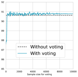
The voting process of classifier can be viewed as a process of taking the expected value of prediction within the vicinity. The law of large numbers is key to understanding the relationship between sample size and expectation. It states that as the sample size increases, the sample mean converges to the true expectation.
To validate this effect empirically, as well as to verify a suitable sample size at which the performance of the voting classifiers can be properly represented, we gradually increase the sample size from 10 to 10,000. As demonstrated in Figure 6, at a small sample size, the voting may result in an increase or a decrease in the performance. However, as the sample exceeds 100, its positive impact on the probabilistic robust accuracy becomes more noticeable. Thus, our empirical intuition matches Theorem 3.2.