Interpretable Price Bounds Estimation with Shape Constraints in Price Optimization

Abstract

This paper addresses the interpretable estimation of price bounds within the context of price optimization. In recent years, price optimization methods have become indispensable for maximizing revenues and profits. However, effectively applying these methods to real-world pricing operations remains a significant challenge. It is crucial for operators, who are responsible for setting prices, to utilize reasonable price bounds that are not only interpretable but also acceptable. Despite this necessity, most studies assume that price bounds are given constant values, and few have explored the reasonable determination of these bounds. In response, we propose a comprehensive framework for determining price bounds, which includes both the estimation and adjustment of these bounds. Specifically, we first estimate the price bounds using three distinct approaches based on historical pricing data. We then adjust the estimated price bounds by solving an optimization problem that incorporates shape constraints. This method allows for the implementation of price optimization under practical and reasonable price bounds, suitable for real-world applications. We report the effectiveness of our proposed method through numerical experiments conducted with historical pricing data from actual services.

1 Introduction

1.1 Background

The prices of products and services have a significant impact on consumer demand, allowing companies to increase revenues and profits through appropriate pricing strategies. Moreover, rapid advancements in information technology and the development of e-commerce have facilitated the integration of real-time consumer demand data into pricing strategies. This integration has increased the impact of pricing strategies on revenues and profits. Consequently, the significance of data-driven price optimization is increasingly being highlighted.

Despite these advancements, many companies continue to rely on the intuition and experience of pricing operators to set prices for products and services. Manual pricing by operators incurs labor costs and is inherently limited in its ability to maximize revenues and profits. Consequently, there is a growing trend towards developing automated pricing systems that optimize revenues and profits by incorporating analyses of customer and competitor responses, sales performance, and pricing trends. Investments in such systems and tools have become particularly prevalent in the retail industry levy2004emerging .

However, their implementation and practical application of these systems in real operations is not straightforward. In practice, although the optimal price suggested by the systems should ideally be adopted as the product price, operators must still take responsibility for setting prices. For example, operators may find it difficult to trust the system if the suggested prices frequently deviate significantly from the prices they have previously set. Therefore, to support effective decision-making, it is essential that these systems propose prices within a range deemed acceptable by operators.

1.2 Related work

Price optimization is a critical decision-making challenge for many organizations and has been extensively studied as a central topic in the field of marketing. Price optimization has been successfully applied across a diverse range of industries, including retail bitran1997periodic ; subrahmanyan1996developing , car rental carroll1995evolutionary ; geraghty1997revenue , hotels bitran1995application ; bitran1996managing , internet providers nair2001application , passenger railways ciancimino1999mathematical , cruise lines ladany1991optimal , and electricity schweppe2013spot ; smith1993linear ; oren1993service ; see also comprehensive surveys klein2020review ; kunz2014demand ; bitran2003overview on revenue management and price optimization.

These price optimization problems are typically designed to derive an optimal price that maximizes revenue or profit within a given price range (i.e., lower and upper price bounds). While many studies assume fixed constant values for price bounds, in real business operations, price bounds vary depending on the product type and the current prices, requiring adaptation according to the situation.

Thus, in real business operations, setting appropriate price bounds for each product is essential. However, to the best of our knowledge, few studies have thoroughly considered or discussed how to determine appropriate price bounds for real-world applications. Consequently, determining the price bounds of products based on historical pricing data remains a critical challenge for making price optimization methods more applicable.

1.3 Our Contribution

The goal of this paper is to establish a framework for determining the price bounds of products in price optimization, using historical pricing data. To this end, we propose an interpretable framework consisting of two phases: estimation and adjustment of price bounds.

First, we introduce three approaches for estimating price bounds based on naive rules (NR), data mining (DM) techniques, and machine learning (ML) techniques. However, due to the limited availability of historical data, these approaches can sometimes lead to overfitting, complicating the interpretation of price bounds by operators. To address this issue, we adjust the estimated price bounds by solving an optimization problem that involves shape constraints such as monotonicity, convexity, and concavity. This problem is formulated as a convex quadratic optimization problem, which can be easily solved using optimization solvers.

To validate the effectiveness of our proposed framework in determining appropriate price bounds, we conducted numerical experiments with actual historical pricing data from Recruit Co., Ltd. We evaluated the accuracy of two methods: one that relies solely on estimation approaches, and another that integrates mathematical optimization with shape constraints. The results of these experiments indicate that our method not only improves the accuracy of price bounds estimation by mitigating overfitting, but also provides highly interpretable price bounds.

2 Problem Setting

In this paper, we focus on the case where the prices of multiple products are optimized simultaneously to maximize revenue. Let $p_{m}$ and $q_{m}$ denote the price and demand of product $m\in\mathcal{M}$, respectively. The price vector is defined as $\bm{p}=(p_{m})_{m\in\mathcal{M}}$. The demand $q_{m}$ for product $m$ depends on both its own price and the prices of other products; hence, it is described as a function of the price vector $\bm{p}$, denoted by $q_{m}(\bm{p})$.

Furthermore, let $\mathcal{P}_{m}$ be the feasible region for the price $p_{m}$. The multi-product price optimization problem can be subsequently formulated as follows soon2011review ; ito2017optimization ; ikeda2023prescriptive :

$$\underset{\bm{p}~{}~{}}{\parbox{50.00008pt}{maximize}} \sum_{m\in\mathcal{M}}p_{m}q_{m}(\bm{p}),$$ (1)

subject to $$~{}p_{m}\in\mathcal{P}_{m},\quad\forall m\in\mathcal{M},$$ (2)

where the objective function (1) represents total revenue, and the constraints (2) ensure that the price $p_{m}$ is selected from a feasible set of prices satisfying operational constraints.

In real-world pricing operations, there are a variety of operational constraints, including price bounds and markup/markdown constraints bitran2003overview . Integrating these constraints into an optimization model is essential for developing a price optimization system that is practically applicable. However, given the diverse range of products, it is often challenging for operators to thoroughly examine these constraints. Operators also frequently rely on their intuition and experience in decision-making, which complicates the explicit definition of these constraints within the model. Consequently, formulating a price optimization problem that fully accounts for all real-world operational constraints becomes particularly challenging. Moreover, even when these constraints can be explicitly defined, their inclusion often makes the optimization problem significantly more complex to solve gallego2019revenue .

To address this issue, we derive the feasible region $\mathcal{P}_{m}$ for the price $p_{m}$ using historical pricing data as a constraint on the price bounds for each current price. In this paper, we focus on determining the profit margin rate driven by cost-based pricing, rather than setting direct prices. Let $c_{m}$ and $r_{m}$ represent the cost and profit margin rate of product $m$, respectively. The price of product $p_{m}$ can then be described as follows:

$$p_{m}=(1+r_{m})\cdot c_{m},\quad\forall m\in\mathcal{M}.$$ (3)

Consequently, the task of estimating the feasible region $\mathcal{P}_{m}$ for the price $p_{m}$ shifts to determining the feasible region $\mathcal{R}_{m}$ for the profit margin rate $r_{m}$.

Fig. 1 shows the real historical pricing data for three products, scaled by a uniform value. The data in the lower right triangle (i.e., the area below the red diagonal line) indicates a decrease in prices, whereas the data in the upper left triangle indicates an increase. This figure also illustrates that the operating range of the profit margin rate highly depends on the current profit margin rate. Moreover, it reveals that the operating ranges of the profit margin rate differ across various product types, even when the current profit margin rates are identical.

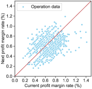
(a) Product A

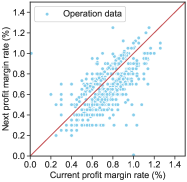
(b) Product B

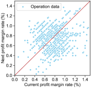
(c) Product C

Figure 1: Real historical pricing data for three products

Therefore, we estimate the bounds of the profit margin rate based on the current profit margin rate. We first discretize the domain of the profit margin rate, $[r^{\min},r^{\max}]$, using a specified step size $\delta$. Let $i\in\mathcal{I}$ denote an index corresponding to a current profit margin rate, with $\mathcal{I}$ defined as $\{1,2,\dots,\lceil(r^{\max}-r^{\min})/\delta\rceil\}$. We define $r^{\text{lb}}_{im}$ and $r^{\text{ub}}_{im}$ as the lower and upper bounds of the profit margin rate for index $i$ and product $m$, respectively. For index $i$ and product $m$, the price bound constraint is equivalent to the following constraint:

$$r^{\text{lb}}_{im}\leq r_{m}\leq r^{\text{ub}}_{im}.$$ (4)

The main purpose of this paper is to determine appropriate bounds of the profit margin rate (i.e., $r^{\text{lb}}_{im}$ and $r^{\text{ub}}_{im}$) using historical pricing data. Note that in subsequent discussions, subscripts denoting product $m$ are omitted because the bounds of the profit margin rate are estimated individually for each product $m$.

3 Our Framework of Interpretable Price Bounds Estimation

In this section, we propose a framework for determining appropriate bounds of the profit margin rate, incorporating both estimation and adjustment processes. First, we present three different estimation approaches, which are based on naive rules, DM techniques, and ML techniques. Subsequently, we detail the adjustment of the estimated bounds via mathematical optimization.

3.1 Price Bounds Estimation

While we have many alternatives to estimate price bounds from two-dimensional pricing data, in this paper, we present three representative estimation approaches: the NR-based approach, the DM-based approach, and the ML-based approach.

NR-Based Approach

First, we estimate the bounds of the profit margin rate using quantiles. Quantiles are values that divide a finite set of data into $q$ subsets of approximately equal size, ensuring that each subset contains approximately the same number of data.

Let $\mathcal{R}_{i}$ denote the set of the next profit margin rates in historical pricing data corresponding to index $i$. We then sort the elements of $\mathcal{R}_{i}$ in ascending order as $\bar{r}_{i1}\leq\bar{r}_{i2}\leq\cdots\leq\bar{r}_{i|\mathcal{R}_{i}|}$. For a real number $q\in[0,1]$, the $q$-quantile $r^{\text{qnt}}_{i}(q)$ of $\mathcal{R}_{i}$ is defined as follows:

$$t =1-q+q|\mathcal{R}_{i}|,$$ (5)

$$r_{i}^{\text{qnt}}(q) =\begin{cases}\bar{r}_{it},&\text{ if }t\in\mathbb{N},\\ (\lceil t\rceil-t)\bar{r}_{i\lfloor t\rfloor}+(t-\lfloor t\rfloor)\bar{r}_{i\lceil t\rceil},&\text{ otherwise }.\end{cases}$$ (6)

Fig. 2 shows an example of estimating the bounds of the profit margin rate using quantiles. In this approach, the $q$-quantile is designated as the estimated lower bound, $\hat{r}^{\text{lb}}_{i}$, and the $1-q$ quantile as the estimated upper bound, $\hat{r}^{\text{ub}}_{i}$, as follows:

$$\hat{r}^{\text{lb}}_{i}=r_{i}^{\text{qnt}}(q),\quad\hat{r}^{\text{ub}}_{i}=r_{i}^{\text{qnt}}(1-q),\quad\forall i\in\mathcal{I}.$$ (7)

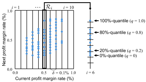
Figure 2: Example of estimated bounds using quantiles

DM-Based Approach

Next, we use association rules to estimate the bounds of the profit margin rate. Association rule mining, proposed by Agrawal et al. agrawal1993mining , is a fundamental technique in data mining. This method excels at extracting rules from large datasets and has been extensively applied across various fields. For instance, it is utilized to analyze relationships between products, as detailed in several comprehensive surveys karthikeyan2014survey ; zhang2010survey ; hipp2000algorithms .

In particular, we use a single association rule for one-dimensional numerical data to estimate the bounds of the profit margin rate (i.e., $r^{\text{lb}}_{i}$ and $r^{\text{ub}}_{i}$) for each index $i$. The performance of association rules is evaluated using two critical metrics: support and confidence.

Analogous to index $i$, let $j\in\mathcal{J}$ denote an index of a profit margin rate subsequent to index $i$ of the current profit margin rate. Additionally, define $[s,t]$ as the index range corresponding to the estimated bounds, $\hat{r}^{\text{lb}}_{i}$ and $\hat{r}^{\text{ub}}_{i}$. Let $v_{ij}$ be a binary value, set to 1 if any operation within the profit margin rate occurs between indices $j$ and $j+1$ for index $i$, and 0 otherwise.

The support, denoted as $\textit{sup}_{i}\in[0,1]$, and the confidence, denoted as $\textit{conf}_{i}\in[0,1]$, for the index range $[s,t]$ corresponding to index $i$ of the current profit margin rate, are then defined as follows:

$$\textit{sup}_{i}=\frac{\sum_{j=s}^{t}v_{ij}}{\sum_{j\in\mathcal{J}}v_{ij}},\quad\forall i\in\mathcal{I},$$ (8)

$$\textit{conf}_{i}=\frac{\sum_{j=s}^{t}v_{ij}}{\sum_{j=s}^{t}1},\quad\forall i\in\mathcal{I}.$$ (9)

The estimated bounds of the profit margin rate, $\hat{r}^{\text{lb}}_{i}$ and $\hat{r}^{\text{ub}}_{i}$, are determined using optimized confidence rules, which are association rules with the highest confidence satisfying the given minimum support. Fig. 3 illustrates an example of estimating the bounds of the profit margin rate using an optimized confidence rule, with the minimum support set to $0.8$.

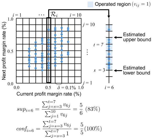
Figure 3: Example of estimated bounds using association rules

ML-Based Approach

Finally, we employ a One-Class SVM scholkopf1999support as a machine learning method to estimate the bounds of the profit margin rate. One-Class SVMs are models primarily used for anomaly detection tasks. This model is designed to train the boundaries that encapsulate the regions within the dataset where samples are predominantly located. It subsequently identifies data that lie outside these predefined boundaries as anomalies.

Let $K$ denote the number of operation data and $k$ denote the index of these data, where each operation point $\bm{x}_{k}$ is characterized by coordinates $(r^{\text{cur}}_{k},r^{\text{next}}_{k})$, representing the current and next profit margin rates, respectively. Let $\bm{w}$ represent the weight vector of the model in the feature space, and let $\phi(\bm{x}_{k})$ denote the function that maps $\bm{x}_{k}$ to a higher dimensional space. Let $\rho$ be the threshold of the discriminant function and $\xi_{k}$ be the slack variable, where $\bm{\xi}=(\xi_{1},\xi_{2},\ldots,\xi_{K})$. The regularization parameter is defined as $\nu$.

The One-Class SVM problem is then formulated as follows:

$$\underset{\bm{w},\bm{\xi},\rho~{}~{}~{}}{\parbox{50.00008pt}{minimize}}~{} \frac{1}{2}|\bm{w}|^{2}+\frac{1}{\nu K}\sum_{k=1}^{K}\xi_{k}-\rho,$$ (10)

subject to $$\langle\bm{w},\phi(\bm{x}_{k})\rangle\geq\rho-\xi_{k},\quad k=1,\ldots,K,$$ (11)

$$\xi_{k}\geq 0,\quad k=1,\ldots,K,$$ (12)

where $\langle\cdot,\cdot\rangle$ denotes the inner product. Furthermore, for the operation data $\bm{x}_{k}$, the anomaly score is calculated as follows:

$$f(\bm{x}_{k})=\operatorname{sgn}(\langle\bm{w},\phi(\bm{x}_{k})\rangle-\rho),$$ (13)

where $\operatorname{sgn}(\cdot)$ denotes the sign function. This function returns $+1$ (indicating normal) if the calculated score exceeds $\rho$, and $-1$ (indicating abnormal) otherwise. The boundary is defined as the point where the output of the function switches from $-1$ to $+1$, or vice versa.

Let $\mathcal{B}_{i}$ denote the set of the next profit margin rates that are located on the boundary corresponding to index $i$. In this approach, the estimated lower bound $\hat{r}^{\text{lb}}_{i}$ and the estimated upper bound $\hat{r}^{\text{ub}}_{i}$ are defined as follows:

$$\hat{r}^{\text{lb}}_{i}=\min\{b\mid b\in\mathcal{B}_{i}\},\quad\hat{r}^{\text{ub}}_{i}=\max\{b\mid b\in\mathcal{B}_{i}\},\quad\forall i\in\mathcal{I}.$$ (14)

3.2 Price Bounds Adjustment

Fig. 4 illustrates the estimated bounds derived using association rules as an example. While these bounds cover most of the historical operations, several issues remain.

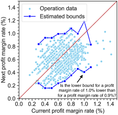
(a) Step size: 0.1% (i.e., $\delta=0.001$)      

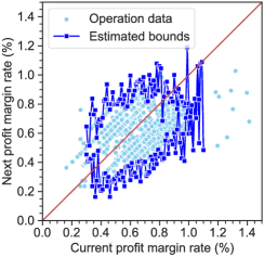
(b) Step size: 0.01% (i.e., $\delta=0.0001$)

Figure 4: Estimated bounds of the profit margin rate using DM-based approach (for the minimum support of 1.0)

As shown in the left figure, the lower bound for the historical profit margin rate of 1.0% is smaller than that for 0.9%, resulting in an inconsistent trend in the estimated bounds that may be difficult for operators to interpret. Furthermore, the sample size varies significantly across the different profit margin rates, which greatly affects the accuracy of the estimated bounds.

In the right-hand figure, where the step size, $\delta$, of the profit margin rate is set to 0.01%, the bounds of the profit margin rate exhibit high volatility and multiple extremes. Such volatility and extremes deviate from operators’ expectations, making it difficult to identify a clear and consistent trend and challenging the effective use of pricing systems.

To address these issues, we employ mathematical optimization to adjust the estimated bounds derived by the aforementioned approaches. During this process, we introduce shape constraints into the optimization problem to reflect the characteristics of pricing operations. The proposed method builds on our previous work iwanaga2016estimating ; nishimura2018latent ; iwanaga2019improving ; nishimura2023predicting , where shape constraints based on prior knowledge were used to estimate product choice probabilities on e-commerce platforms.

We introduce three shape constraints to reflect the following properties of pricing operations:

• Monotonicity: Both the lower and upper bounds of the profit margin rate are adjusted to increase monotonically as the current profit margin rate increases.

• Convexity of Lower Bounds: The rate of increase for the lower bound of the profit margin rate accelerates as the current profit margin rate increases.

• Concavity of Upper Bounds: The rate of increase for the upper bound of the profit margin rate decelerates as the current profit margin rate increases.

Let $\hat{r}_{i}^{\text{lb}}$ and $\hat{r}_{i}^{\text{ub}}$ denote the estimated lower and upper bounds of the profit margin rate, respectively, as obtained using the estimation approaches described in Section 3.1. Additionally, let $w_{i}$ represent the weight coefficient for index $i$, defined in this paper as the number of data for index $i$, and let $r_{i}^{\text{lb}}$ and $r_{i}^{\text{ub}}$ denote the adjusted lower and upper bounds, respectively. The vector of these adjusted bounds is defined as $\bm{r}^{\text{lb}}=(r_{i}^{\text{lb}})_{i\in\mathcal{I}}$ and $\bm{r}^{\text{ub}}=(r_{i}^{\text{ub}})_{i\in\mathcal{I}}$.

The optimization problem for adjusting the estimated bounds can be formulated as a convex quadratic optimization problem, incorporating the aforementioned properties of pricing operations, as follows:

$$\underset{\bm{r}^{\text{lb}},\bm{r}^{\text{ub}}}{\parbox{50.00008pt}{minimize}}~{} \sum_{i\in\mathcal{I}}w_{i}\Bigl{\{}(r_{i}^{\text{lb}}-\hat{r}_{i}^{\text{lb}})^{2}+(r_{i}^{\text{ub}}-\hat{r}_{i}^{\text{ub}})^{2}\Bigr{\}},$$ (15)

subject to $$r_{i-1}^{\text{lb}}\leq r_{i}^{\text{lb}},\quad\forall i\in\mathcal{I}\backslash\{1\},$$ (16)

$$r_{i-1}^{\text{ub}}\leq r_{i}^{\text{ub}},\quad\forall i\in\mathcal{I}\backslash\{1\},$$ (17)

$$r_{i}^{\text{lb}}-r_{i-1}^{\text{lb}}\geq r_{i-1}^{\text{lb}}-r_{i-2}^{\text{lb}},\quad\forall i\in\mathcal{I}\backslash\{1,2\},$$ (18)

$$r_{i}^{\text{ub}}-r_{i-1}^{\text{ub}}\leq r_{i-1}^{\text{ub}}-r_{i-2}^{\text{ub}},\quad\forall i\in\mathcal{I}\backslash\{1,2\},$$ (19)

$$r_{i}^{\text{lb}}\leq r_{i}^{\text{ub}},\quad\forall i\in\mathcal{I},$$ (20)

where the objective function (15) represents the weighted sum of the squares of the differences between the estimated and adjusted lower and upper bounds of the profit margin rate. The constraints (16) and (17) ensure the monotonicity of the lower and upper bounds, respectively. The constraints (18) and (19) impose convexity on the lower bound and concavity on the upper bound, respectively. Finally, the constraint (20) guarantees that the lower bound remains below the upper bound.

4 Numerical Experiments

In this section, we evaluate the effectiveness of our framework for estimating interpretable price bounds through numerical experiments conducted on historical pricing data from real services.

4.1 Experimental Design

In our experiments, we used real pricing data for three main products offered by Recruit Co., Ltd. for the period from January 1, 2019, to December 31, 2019. In this paper, these products are referred to as Product A, Product B, and Product C. We also set the minimum and maximum values of the current profit margin rate at 0.3% and 1.1%, respectively (i.e., $r^{\text{min}}=0.003,r^{\text{max}}=0.011$). The domain $[r^{\text{min}},r^{\text{max}}]$ of the current profit margin rate covers more than $97\%$ of all operations.

To evaluate the proposed method, we employed cross-validation and divided the data into five folds based on the operation date for each pricing operation. Subsequently, for each estimation approach (i.e., NR-based, DM-based, and ML-based approaches), we compared the Root Mean Squared Error (RMSE) between the estimated values without adjustment and those with adjustment for four different methods:

NA:

No adjustment i.e., price bounds estimation only;

MN:

Monotonicity adjustment only;

CC:

Convexity-concavity adjustment only;

MN-CC:

Both monotonicity and convexity-concavity adjustments.

To validate the effectiveness of the proposed method, we define the improvement rate as follows:

$$\text{Improvement rate~{}(\%)}=100\cdot\biggl{(}1-\frac{\text{RMSE of the best method}}{\text{RMSE of NA}}\biggr{)}.$$ (21)

Additionally, we consider two cases for the step size: 0.1% and 0.01% (i.e., $\delta$ values of 0.001 and 0.0001, respectively). The hyperparameters for each estimation approach were set as follows, with other hyperparameters maintained at their default values:

• For the NR-based approach, the parameter $q$ was set to $\{0.00,0.05,0.10\}$.

• For the DM-based approach, the minimum support was set to $\{0.8,0.9,1.0\}$.

• For the ML-based approach, the regularization parameter $\nu$ was set to $\{0.01,0.03,0.05\}$.

In the NR-based approach, quantiles were calculated using the quantile function from Numpy 1.24.2, a Python library designed for efficient numerical calculations. In the ML-based approach, One-Class SVM models were implemented using the OneClassSVM function in scikit-learn 1.2.2 pedregosa2011scikit , a comprehensive Python library for machine learning tools. The quadratic optimization problem was solved using OSQP version 0.6.1, a state-of-the-art solver for continuous optimization.

4.2 Results and Discussion

Tables 1, 2, and 3 show the estimation errors derived from the NR-based approach, the DM-based approach, and the ML-based approach, respectively. Both the NR-based and DM-based approaches exhibit similar trends, with the errors arranged in ascending order as follows: MN-CC, CC, MN, and NA.

Conversely, for the ML-based approach (i.e., Table 3), the errors are ranked in ascending order: CC, NA, MN-CC, and MN. This ranking results from the tendency for the One-Class SVM to initially generate a boundary for our pricing data that closely approximates the shape of the convex hull.

Therefore, although the appropriate shape constraints need to be selected based on the estimation approach, these results indicate that for various estimation approaches, the shape constraints improve the accuracy of the price bounds estimation. Note also that the improvement rates in Tables 1 and 2 are calculated for MN-CC and those in Table 3 are calculated for CC.

Table 1: RMSE by using NR-based approach

Step size	$q$	Product	NA	MN	CC	MN-CC	Improvement
0.01%	0.00	A	0.193	0.181	0.184	0.182	5.7%
		B	0.186	0.172	0.174	0.174	6.4%
		C	0.295	0.274	0.275	0.273	7.5%
0.01%	0.05	A	0.176	0.159	0.162	0.159	9.5%
		B	0.169	0.149	0.150	0.149	11.8%
		C	0.284	0.259	0.261	0.258	9.1%
0.01%	0.10	A	0.173	0.155	0.158	0.155	10.7%
		B	0.156	0.136	0.137	0.136	13.0%
		C	0.285	0.252	0.256	0.252	11.7%
0.1%	0.00	A	0.191	0.194	0.175	0.179	6.6%
		B	0.214	0.195	0.192	0.186	13.1%
		C	0.289	0.287	0.276	0.274	5.2%
0.1%	0.05	A	0.150	0.141	0.132	0.131	13.2%
		B	0.156	0.149	0.130	0.131	16.2%
		C	0.194	0.193	0.170	0.175	10.1%
0.1%	0.10	A	0.146	0.134	0.129	0.125	14.3%
		B	0.131	0.127	0.119	0.118	9.5%
		C	0.193	0.187	0.167	0.168	13.1%
Average			0.199	0.186	0.180	0.179	10.0%

Table 2: RMSE by using DM-based approach

Step size	Min. support	Product	NA	MN	CC	MN-CC	Improvement
0.01%	0.8	A	0.143	0.121	0.120	0.119	16.2%
		B	0.131	0.120	0.118	0.118	9.5%
		C	0.190	0.165	0.165	0.163	14.2%
0.01%	0.9	A	0.145	0.131	0.129	0.129	10.5%
		B	0.153	0.136	0.136	0.136	11.3%
		C	0.209	0.180	0.180	0.179	14.3%
0.01%	1.0	A	0.161	0.149	0.149	0.148	7.6%
		B	0.166	0.148	0.149	0.149	10.3%
		C	0.223	0.200	0.200	0.199	10.7%
0.1%	0.8	A	0.092	0.091	0.090	0.091	0.7%
		B	0.115	0.118	0.113	0.115	-0.1%
		C	0.159	0.143	0.147	0.138	13.6%
0.1%	0.9	A	0.107	0.105	0.102	0.102	4.8%
		B	0.144	0.141	0.136	0.135	6.3%
		C	0.185	0.173	0.164	0.154	16.3%
0.1%	1.0	A	0.150	0.157	0.144	0.149	7.6%
		B	0.206	0.183	0.189	0.181	12.0%
		C	0.272	0.269	0.263	0.263	4.8%
Average			0.164	0.152	0.150	0.148	9.6%

Table 3: RMSE by ML-based approach

Step size	$\nu$	Product	NA	MN	CC	MN-CC	Improvement
0.01%	0.01	A	0.095	0.100	0.091	0.097	4.5%
		B	0.119	0.120	0.119	0.121	0.0%
		C	0.215	0.217	0.215	0.217	0.0%
0.01%	0.03	A	0.087	0.093	0.086	0.092	1.1%
		B	0.056	0.062	0.056	0.061	0.1%
		C	0.176	0.180	0.173	0.179	1.6%
0.01%	0.05	A	0.101	0.104	0.095	0.100	6.2%
		B	0.062	0.068	0.062	0.068	0.1%
		C	0.153	0.154	0.146	0.152	4.1%
0.1%	0.01	A	0.160	0.162	0.151	0.157	5.2%
		B	0.126	0.129	0.126	0.129	0.0%
		C	0.234	0.241	0.234	0.231	0.0%
0.1%	0.03	A	0.113	0.117	0.125	0.123	-10.2%
		B	0.091	0.103	0.091	0.103	0.0%
		C	0.207	0.206	0.200	0.204	3.4%
0.1%	0.05	A	0.111	0.112	0.129	0.121	-15.7%
		B	0.093	0.108	0.093	0.108	0.0%
		C	0.157	0.165	0.155	0.161	1.6%
Average			0.131	0.136	0.130	0.135	0.1%

Figs. 5, 6, and 7 show the estimated bounds of the profit margin rate for Product A, derived using the NR-based approach, the DM-based approach, and the ML-based approach, respectively, with step sizes set to $0.01\%$.

In particular, when the step size is set to $0.01\%$ for both the rule-based approach and DM-based approaches, as shown in Figs. 5 and 6, the estimated bounds fluctuate considerably without adjustment, making it difficult for operators to interpret the trends. It can be observed that these estimation approaches manage to avoid overfitting through the use of shape constraints.

On the other hand, the ML-based approach estimates the bounds based on all historical pricing data and is less susceptible to variation due to smaller sample sizes. However, even in such cases, it is evident that the application of shape constraints corrects the estimated bounds to more appropriate and easily interpretable levels.

(a) NA

(b) MN

(c) CC

(d) MN-CC

Figure 5: Estimated bounds of the profit margin rate for Product A using NR-based approach ($q=0.00$) with the step size of $0.01\%$

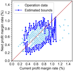
(a) NA

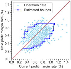
(b) MN

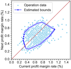
(c) CC

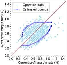
(d) MN-CC

Figure 6: Estimated bounds of the profit margin rate for Product A using DM-based approach with the minimum support of $1.0$ and the step size of $0.01\%$

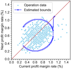
(a) NA

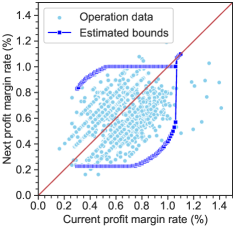
(b) MN

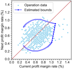
(c) CC

(d) MN-CC

Figure 7: Estimated bounds of the profit margin rate for Product A using ML-based approach ($\nu=0.01$) with the step size of $0.01\%$

Tables 1, 2 and 3 illustrate that under both monotonicity and convexity-concavity adjustments (i.e., MN-CC), the RMSE decreases in the order: ML-based approach ¡ DM-based approach ¡ NR-based approach. However, because the profit margin rate bounds estimated by the ML-based approach did not conform to the operator’s intuition, the DM-based approach was selected for implementation in the actual service.

Fig. 8 presents the results of adjusting the bounds of the profit margin rate for each product derived from the DM-based approach, by incorporating both monotonicity and convexity-concavity constraints. The proposed adjustment approach facilitates the following interpretations of the trends in the profit margin rate bounds:

• Product A: Generally, both the lower and upper bounds of the profit margin rate vary in accordance with the current profit margin rate. However, when the current profit margin rate exceeds approximately 0.6%, the upper bounds tend to be suppressed. Conversely, when the rate falls below this threshold, the lower bounds are similarly restrained.

• Product B: Both the lower and upper bounds of the margin rate are tight. In particular, the upper bounds tend to be restrictive, resulting in infrequent price increases.

• Product C: The lower bounds of the profit margin rate are independent of the current profit margin up to approximately 0.8%; for higher profit margins, the lower bounds increase in proportion to the current profit margin rates. The increase in the upper bounds becomes slower around 0.4% and is less sensitive to changes in the current profit margin rate.

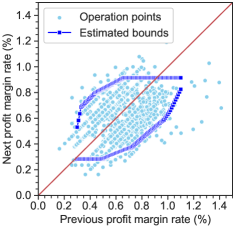
(a) Product A

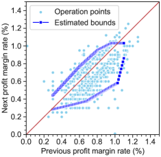
(b) Product B

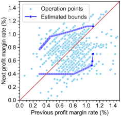
(c) Product C

Figure 8: Estimated bounds of the profit margin rate for each product using DM-based approach with the minimum support of 1.0 and the step size of $0.01\%$

5 Conclusion

We propose an interpretable framework for determining price bounds that consists of two main components: price bounds estimation and adjustment using historical pricing data. First, we introduce three approaches for estimating the bounds of the profit margin rate: an NR-based approach, a DM-based approach, and an ML-based approach. Subsequently, we present a method for adjusting these estimated bounds through mathematical optimization.

In numerical experiments using real pricing data from Recruit Co., Ltd., we found that the proposed method not only improved estimation accuracy, but also that the adjusted bounds increased stability and were less susceptible to outliers, making them highly practical and easier for operators to interpret. These improvements are expected to strengthen the validity of pricing strategies and facilitate more strategic decision-making by providing clearer insights into pricing practices.

A segment of our framework, specifically the estimation using the DM-based approach coupled with adjustments via mathematical optimization, was actually implemented in the price optimization system at Recruit Co., Ltd. This implementation significantly facilitated the seamless integration of the price optimization system into actual pricing operations, aiding in the interpretation of price bounds. Consequently, this led to considerable savings in labor costs for pricing operations and an increase in the revenue and profits of the services.

References

- (1) Agrawal, R., Imieliński, T., Swami, A.: Mining association rules between sets of items in large databases. In: Proceedings of the 1993 ACM SIGMOD international conference on Management of data, pp. 207–216 (1993)
- (2) Bitran, G., Caldentey, R.: An overview of pricing models for revenue management. Manufacturing & Service Operations Management 5(3), 203–229 (2003)
- (3) Bitran, G.R., Gilbert, S.M.: Managing hotel reservations with uncertain arrivals. Operations Research 44(1), 35–49 (1996)
- (4) Bitran, G.R., Mondschein, S.V.: An application of yield management to the hotel industry considering multiple day stays. Operations Research 43(3), 427–443 (1995)
- (5) Bitran, G.R., Mondschein, S.V.: Periodic pricing of seasonal products in retailing. Management Science 43(1), 64–79 (1997)
- (6) Carroll, W.J., Grimes, R.C.: Evolutionary change in product management: Experiences in the car rental industry. Interfaces 25(5), 84–104 (1995)
- (7) Ciancimino, A., Inzerillo, G., Lucidi, S., Palagi, L.: A mathematical programming approach for the solution of the railway yield management problem. Transportation Science 33(2), 168–181 (1999)
- (8) Gallego, G., Topaloglu, H.: Revenue management and pricing analytics, vol. 209. Springer, New York (2019)
- (9) Geraghty, M.K., Johnson, E.: Revenue management saves national car rental. Interfaces 27(1), 107–127 (1997)
- (10) Hipp, J., Güntzer, U., Nakhaeizadeh, G.: Algorithms for association rule mining—a general survey and comparison. ACM SIGKDD explorations newsletter 2(1), 58–64 (2000)
- (11) Ikeda, S., Nishimura, N., Sukegawa, N., Takano, Y.: Prescriptive price optimization using optimal regression trees. Operations Research Perspectives 11, 100290 (2023)
- (12) Ito, S., Fujimaki, R.: Optimization beyond prediction: Prescriptive price optimization. In: Proceedings of the 23rd ACM SIGKDD international conference on knowledge discovery and data mining, pp. 1833–1841 (2017)
- (13) Iwanaga, J., Nishimura, N., Sukegawa, N., Takano, Y.: Estimating product-choice probabilities from recency and frequency of page views. Knowledge-Based Systems 99, 157–167 (2016)
- (14) Iwanaga, J., Nishimura, N., Sukegawa, N., Takano, Y.: Improving collaborative filtering recommendations by estimating user preferences from clickstream data. Electronic Commerce Research and Applications 37, 100877 (2019)
- (15) Karthikeyan, T., Ravikumar, N.: A survey on association rule mining. International Journal of Advanced Research in Computer and Communication Engineering 3(1), 2278–1021 (2014)
- (16) Klein, R., Koch, S., Steinhardt, C., Strauss, A.K.: A review of revenue management: Recent generalizations and advances in industry applications. European Journal of Operational Research 284(2), 397–412 (2020)
- (17) Kunz, T.P., Crone, S.F.: Demand models for the static retail price optimization problem-a revenue management perspective. In: 4th Student conference on operational research. Schloss Dagstuhl-Leibniz-Zentrum fuer Informatik (2014)
- (18) Ladany, S.P., Arbel, A.: Optimal cruise-liner passenger cabin pricing policy. European Journal of Operational Research 55(2), 136–147 (1991)
- (19) Levy, M., Grewal, D., Kopalle, P.K., Hess, J.D.: Emerging trends in retail pricing practice: implications for research. Journal of Retailing 80(3), xiii–xxi (2004)
- (20) Nair, S.K., Bapna, R.: An application of yield management for internet service providers. Naval Research Logistics (NRL) 48(5), 348–362 (2001)
- (21) Nishimura, N., Sukegawa, N., Takano, Y., Iwanaga, J.: A latent-class model for estimating product-choice probabilities from clickstream data. Information Sciences 429, 406–420 (2018)
- (22) Nishimura, N., Sukegawa, N., Takano, Y., Iwanaga, J.: Predicting online item-choice behavior: A shape-restricted regression approach. Algorithms 16(9), 415 (2023)
- (23) Oren, S.S., Smith, S.A.: Service Opportunities for Electric Utilities: Creating Differentiated Products: Creating Differentiated Products;[papers Presented at a Symposium Held at the University of California at Berkeley, Sept. 12-14, 1990], vol. 13. Springer Science & Business Media, Heidelberg (1993)
- (24) Pedregosa, F., Varoquaux, G., Gramfort, A., Michel, V., Thirion, B., Grisel, O., Blondel, M., Prettenhofer, P., Weiss, R., Dubourg, V., et al.: Scikit-learn: Machine learning in python. The Journal of Machine Learning Research 12, 2825–2830 (2011)
- (25) Schölkopf, B., Williamson, R.C., Smola, A., Shawe-Taylor, J., Platt, J.: Support vector method for novelty detection. Advances in Neural Information Processing Systems 12 (1999)
- (26) Schweppe, F.C., Caramanis, M.C., Tabors, R.D., Bohn, R.E.: Spot pricing of electricity. Springer Science & Business Media, Heidelberg (2013)
- (27) Smith, S.A.: A linear programming model for real-time pricing of electric power service. Operations Research pp. 470–483 (1993)
- (28) Soon, W.: A review of multi-product pricing models. Applied Mathematics and Computation 217(21), 8149–8165 (2011)
- (29) Subrahmanyan, S., Shoemaker, R.: Developing optimal pricing and inventory policies for retailers who face uncertain demand. Journal of Retailing 72(1), 7–30 (1996)
- (30) Zhang, M., He, C.: Survey on association rules mining algorithms. Advancing Computing, Communication, Control and Management pp. 111–118 (2010)