DETAIL: Task DEmonsTration Attribution for Interpretable In-context Learning

Abstract

In-context learning (ICL) allows transformer-based language models that are pre-trained on general text to quickly learn a specific task with a few “task demonstrations” without updating their parameters, significantly boosting their flexibility and generality. ICL possesses many distinct characteristics from conventional machine learning, thereby requiring new approaches to interpret this learning paradigm. Taking the viewpoint of recent works showing that transformers learn in context by formulating an internal optimizer, we propose an influence function-based attribution technique, DETAIL, that addresses the specific characteristics of ICL. We empirically verify the effectiveness of our approach for demonstration attribution while being computationally efficient. Leveraging the results, we then show how DETAIL can help improve model performance in real-world scenarios through demonstration reordering and curation. Finally, we experimentally prove the wide applicability of DETAIL by showing our attribution scores obtained on white-box models are transferable to black-box models in improving model performance.

1 Introduction

The rapid development of transformer-based language models [10, 12, 15] has inspired a new in-context learning (ICL) paradigm [12], which allows a language model sufficiently pre-trained on general text to quickly adapt to specific tasks. This lightweight approach of customizing a general model for specific tasks is in contrast to fine-tuning [25, 52] that necessitates both access to the model parameters and resource-intensive step of tuning these parameters for model adaptation. In ICL, a few task demonstrations are included in the input text (i.e., prompt) together with a query to help the language model better understand how to answer the query. It has been shown that including task demonstrations in the prompt can enhance the capability of language models to apply common sense and logical reasoning [50, 54] and learn patterns from the supplied demonstrations [12], significantly enhancing the flexibility and generality of language models. In the ICL paradigm, each demonstration can be viewed as a “training data point” for ICL. Analogous to how the performance of a conventional supervised machine learning (ML) model depends on the quality of training data, the performance of ICL depends on the quality of task demonstrations [31]. A research question naturally arises: How to attribute and interpret ICL demonstrations that are helpful or harmful for model prediction?

Though there are many prior works on interpreting and attributing model prediction for conventional ML models [21, 27, 41], these methods are not readily applicable to ICL due to its unique characteristics. Firstly, many existing attribution techniques require either computing the gradients [45] or multiple queries to the model [17], both of which are slow and computationally expensive. In contrast, ICL is often applied in real-time to a large foundation model [10] that necessitates the attribution approaches for ICL to be fast and efficient. Secondly, ICL is known to be sensitive to ordering: The same set of demonstrations can result in significantly different model performance under different permutations [32, 34]. However, conventional methods do not explicitly consider the ordering of training examples. Thirdly, ICL demonstration is usually supplied as a sentence comprising a sequence of tokens, rendering conventional token-level attribution methods ineffective, as they do not capture contextual information of each ICL demonstration [6, 45]. Lastly, ICL does not update model parameters, rendering conventional techniques that analyze model parameter change [27] not applicable. Moreover, the absence of the need to update model parameters also allows a good attribution result for ICL to be transferable across different language models.

To address these challenges, we propose DETAIL, a novel technique that takes advantage of a classical attribution approach while tackling the unique characteristics of ICL. We adopt the perspective that transformers formulate an internal optimizer [3, 14, 47, 53] for ICL. Based on this internal optimizer, we design a method to understand the impact of each demonstration on the transformer’s prediction. Notably, this approach allows us to leverage powerful existing analysis tools for transformer-based models in ICL, where otherwise the characteristics of ICL make applying these tools difficult.

Specifically, we describe an intuitive (re-)formulation of the influence function [27], a popular attribution method for conventional ML, on the internal optimizer and show that DETAIL addresses the challenges of computational cost, sensitivity to order, and attribution quality. Then, we empirically verify that our formulation can identify demonstrations helpful for model prediction and outlier demonstrations. Additionally, we apply our method to tasks with real-world implications including prompt reordering, noisy demonstration detection, and demonstration curation to show its effectiveness. We demonstrate that DETAIL achieves improved performance when applied to typical white-box large language models (LLMs). Furthermore, as many powerful LLMs are currently closed-source (thus black-box), we show that our DETAIL score obtained on a white-box LLM (e.g., Vicuna-7b [59]) exhibits transferable characteristics to the performance on a popular black-box model (ChatGPT).

2 Related Work

Understanding in-context learning.

Prior works have attempted to understand the ICL capability of transformer-based language models [2, 3, 12, 20, 30, 39, 47, 53, 56]. [12] empirically demonstrated that language models can act as few-shot learners for unseen NLP tasks. [39] explained ICL by viewing attention heads as implementing simple algorithms for token sequence completion. [53] studied the ICL capability of transformers by casting it as an implicit Bayesian inference. [3, 20] further showed that transformers can learn (regularized) linear functions in context. [30] provided a statistical generalization bound for in-context learning. [47, 48, 56] mathematically showed that transformers with specific parameters can perform gradient descent on parameters of an internal optimizer given the demonstrations. [2, 56] further proved that the parameters (of the internal optimizer) can converge during forward passing. Inspired by the theoretical grounding, which is the focus of these works, we design our novel attribution technique for task demonstrations by adopting a similar view (i.e. transformers learn in context by implementing an optimization algorithm internally).

Data attribution.

Past works have focused on explaining and attributing model performance to training data of conventional ML [7, 17, 21, 22, 27, 41]. The rise of LLMs has inspired research efforts on attribution w.r.t. prompts with a focus on task demonstrations [9, 33, 35, 43, 55], which is distinct from training data attribution since demonstrations are provided in context. Specifically, [33] used human annotators to evaluate the verifiability of attributing model answers to a prompt. [9, 55] relied on LLMs to evaluate attribution errors. These prior works are either computationally heavy (requiring additional queries of LLMs) or time-consuming (requiring human annotators). [43] proposed an interpretability toolkit for sequence generation models using gradient- and perturbation-based methods. [35], a contemporary work, proposed to use a decoder module on the token embeddings for per-token attribution but requires costly training to learn the decoder weights. Moreover, these methods do not specifically target demonstration attribution. Some prior techniques [17, 21] can be adapted for attributing ICL in LLMs but may be costly or ineffective. We empirically compare our method with those and the attribution methods consolidated in [43].

Using influence in LLMs.

Past works have attempted to apply the notion of influence in language models [22, 28, 38, 42, 52, 57]. [38] considered a simplification of the influence function for task demonstration curation. [22, 28, 52] applied influence to pre-training and fine-tuning data of LLMs. [57] used influence to select demonstration inputs for annotation. [42] builds a classifier on the embeddings of demonstrations using a small LLM and computes influence w.r.t. the classifier for demonstration selection. In contrast, we demonstrate various use cases of our method including on-the-fly demonstration curation, reordering, and noisy demonstration detection. A contemporary work that shares technical similarity [42] focuses on demonstration selection whereas we focus on attribution and  [42] is shown to be less effective than our method in Sec. 5.3. Additionally, compared to prior works leveraging influence to address specific problems, we apply influence function to provide a general attribution for demonstrations, with many applications that we empirically show.

3 Preliminaries

In-context learning (ICL).

ICL is a learning paradigm that provides a few task demonstrations with formatted input and output for a pre-trained transformer (e.g., an LLM) to learn the mapping function from inputs to outputs in context (i.e., via the forward pass) [12]. Formally, a transformer model $f$ takes in a prompt $p(\mathcal{S},x_{\text{query}})$ comprising a formatted sequence of demonstrations $\mathcal{S}=(z_{1},z_{2},\dots,z_{n})$ where $z_{i}=\{x_{i},y_{i}\}$ from a specific downstream task along with a query input $x_{\text{query}}$ (i.e., prompt) to predict its label as $\hat{y}_{\text{query}}=f(p(\mathcal{S},x_{\text{query}}))$. An visual for an example prompt is provided in App. C. We wish to attribute the model prediction $\hat{y}_{\text{query}}$ to each $z_{i}\in\text{set}(\mathcal{S})$.

ICL as implementing an internal optimizer.

With the growing interest in the internal mechanism of transformers, previous works [3, 47, 48, 56] have theoretically shown that ICL can be treated as the transformer implementing an internal optimizer on the ICL demonstrations. Specifically, [47, 48, 56] formulated the objective of ICL optimizer with (regularized) mean-squared error on a linear weight applied to the token itself in linear self-attentions (LSAs) [56] or a transformation of tokens (i.e., kernelized mean-squared error) if an extra multi-layered perception is attached before the LSA [47, Proposition 2] in a recurrent transformer architecture. The transformer layers then function as performing gradient descent on the weight to minimize the objective [47, 56].

Influence function.

Influence function [27] approximates the change of the loss of a test data point $z_{\text{test}}$ when up-weighting a training data point $z_{i}$. Formally, the influence of $z_{i}$ on predicting $z_{\text{test}}$ is

$$\textstyle\mathcal{I}(z_{i},z_{\text{test}})\coloneqq\nabla_{\theta}L(z_{\text{test}},\hat{{\theta}})^{\top}\mathcal{I}_{\text{reg}}(z_{i})=\nabla_{\theta}L(z_{\text{test}},\hat{{\theta}})^{\top}H^{-1}_{\hat{\theta}}\nabla_{\theta}L(z_{i},\hat{\theta})$$ (1)

where $L(z_{\text{test}},\hat{\theta})$ refers to the loss (function) on a test point $z_{\text{test}}$ of the model parameterized by $\hat{{\theta}}$ and $H_{\hat{\theta}}\coloneqq 1/n\sum_{i=1}^{n}\nabla_{\theta}^{2}L(z_{i},\hat{\theta})$ is the Hessian. However, this definition cannot be directly applied to ICL since there is no model parameter change during ICL, unlike the learning settings in [7, 27]. We show how to adapt the formulation of Eq. 1 to ICL in our proposed method DETAIL next.

4 Influence Function on Internal Kernel Regression

Following the idea that transformers learn in context by implementing an internal kernelized least-square objective, we present our formulation of DETAIL by computing the influence function on a kernelized linear regression [24]. Specifically, we build the regression w.r.t. the following kernel

$$\textstyle k(x,x^{\prime})\coloneqq m(x)^{\top}m(x^{\prime})$$ (2)

where $m(x)\in\mathbb{R}^{1\times d}$ refers to (the mapping of an ICL demonstration to) an internal representation of $x$ (e.g., hidden state of a transformer layer) with output dimension $d$. Let $X\coloneqq(x_{1},x_{2},\cdots,x_{n})$ and $Y\coloneqq(y_{1},y_{2},\cdots,y_{n})$ be the vectors of inputs and outputs in $\mathcal{S}$ respectively. The equivalent kernel regression can be written as $\textstyle\hat{Y}\coloneqq m(X)\beta$ where $\beta\in\mathbb{R}^{d\times 1}$ is the weight vector over the kernelized feature space. In practice, the dimension $d$ of $m$ is usually much larger than the number of demonstrations, causing severe over-parameterization. Such over-parameterization renders the influence values fragile [8]. As such, we follow [8] and adopt an $\ell_{2}$ regularization on $\beta$ controlled by a hyper-parameter $\lambda$, which forms a kernelized ridge regression [37] with loss:

$$\textstyle L(x,y)=[m(x)\beta-y]^{2}+\lambda\beta^{\top}\beta\ .$$ (3)

Taking the $2$nd derivative of Eq. 3, we obtain the hessian $H_{\beta}$ as

$$\textstyle H_{\beta}\coloneqq(1/n)\sum_{i=1}^{n}\nabla_{\beta}^{2}L(x_{i},y_{i})=(2/n)\sum_{i=1}^{n}\left(m(x_{i})^{\top}m(x_{i})+\lambda I\right)\ .$$ (4)

Adopting a matrix multiplication form for the summation in Eq. 4, we write the influence of training data on the model parameters $\beta$ as follows,

$$\textstyle\mathcal{I}_{\text{reg}}(z)\coloneqq H_{\beta}^{-1}\nabla_{\beta}L(x,y)=n(K+\lambda I)^{-1}[m(x)^{\top}(m(x)\beta-y)+\lambda\beta]$$ (5)

where $K\coloneqq m(X)^{\top}m(X)\in\mathbb{R}^{d\times d}$ is the Gram matrix and $\mathcal{I}_{\text{reg}}\in\mathbb{R}^{d}$ refers to the influence of a particular demonstration $(x,y)$ w.r.t. the kernel regression weights $\beta$. Then, combining Eqs. 1, 3 and 5, we can express the DETAIL score as the influence of a demonstration $z$ on a query $z_{\text{test}}$:

$$\mathcal{I}(z_{\text{test}},z)\coloneqq\nabla_{\beta}L(x_{\text{test}},y_{\text{test}})^{\top}\mathcal{I}_{\text{reg}}(z)$$ (6)

$$=n[m(x_{\text{test}})^{\top}(m(x_{\text{test}})\beta-y_{\text{test}})+\lambda\beta](K+\lambda I)^{-1}[m(x)^{\top}(m(x)\beta-y)+\lambda\beta]$$

where $\beta$ has a closed-form expression (shown in Alg. 1 in App. B). While inverting matrices in Eq. 6 requires $\mathcal{O}(d^{3})$ time, $d$ is usually in the thousands: A typical LLM like Llama-2-7b [46] has an embedding size $d=4096$, allowing reasonable computation time of $\mathcal{I}$ (e.g., a few seconds). In practice, this computation is accelerated by the techniques already implemented in existing scientific computation libraries admitting sub-cubic complexity for matrix inversion.

Computing self-influence.

One important application of the influence function in ML is identifying outliers via self-influence [7, 27]. The conventional definition of $\mathcal{I}$ trivially admits computing self-influence simply by replacing $z_{\text{test}}$ in Eq. 1 with $z_{i}$. While the same approach applies to DETAIL, there are two shortcomings: (i) As the embedding is sensitive to the position, placing the same demonstration at the end of the prompt (as a query) or in the middle (as a demonstration) results in different embeddings, leading to unreasonable influence score. (ii) For each demonstration, it needs one forward pass of the model to compute the self-influence, which can be costly when the ICL dataset size is large. Instead, we implement self-influence for DETAIL by reusing the demonstration’s embedding. This way, we keep the two sides of Eq. 1 consistent and only require one forward pass of the model to compute the self-influence for all demonstrations.

Further speedup via random matrix projection.

While the current formulation in Eq. 6 is already computationally cheap, a relatively large embedding size (e.g. $d=4096$ for Llama-2-7b) can become a bottleneck as inverting the matrix can be relatively slow. We apply an insight that for ICL, much of the information in the embedding $m$ is redundant (we do not need a $4096$-dimensional $\beta$ to fit $20$ demonstrations). Hence, we project $m$ to a much lower dimensional space via a random matrix projection while preserving the necessary information, following the Johnson-Lindenstrauss lemma [18, 26], precisely represented as a projection matrix $P\in\mathbb{R}^{d\times d^{\prime}}$ with each entry i.i.d. from $\mathcal{N}(0,1/d^{\prime})$. We provide a more detailed discussion in App. C. Empirically, we show that we can compress $m$ to a much smaller dimension $d^{\prime}\leq 1000$, resulting in a $10\times$ computation speedup on a typical 7B LLM on an NVIDIA L40 GPU (see Sec. 5.2).

A visualization of our proposed method is in Fig. 1 and a pseudo-code implementation is in App. B.

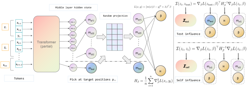
Figure 1: Illustration of computing DETAIL score for transformer-based ICL. Note that we use the same notation $m_{p[\cdot]}$ before and after the random projection since the projection is optional.

5 Empirical Evaluation

We evaluate the effectiveness of DETAIL (i.e., Eq. 6) on two metrics: computational time (via logged system time required) and effectiveness in attribution (via performance metrics for tasks). We start by visualizing how the DETAIL scores, particularly $\mathcal{I}(z_{\text{test}},z_{i})$ (test influence, abbreviated as $\mathcal{I}_{\text{test}}$) and $\mathcal{I}(z_{i},z_{i})$ (self influence, abbreviated as $\mathcal{I}_{\text{self}}$) following [27, Sections 5.1 & 5.4], attribute demonstrations to a query first on a custom transformer and then on LLMs. Note that the hyper-parameter $\lambda$ varies under different scenarios and we discuss some heuristics for setting $\lambda$ in App. C.

Enforcing ICL behavior.

We consider tasks where transformers learn from the demonstrations and form an internal optimizer. To evaluate the effectiveness of our method, we enforce the ICL behavior by mapping the labels of the demonstrations to a token that carries no semantic meaning, This way, pre-trained transformers cannot leverage memorized knowledge to produce answers but have to learn the correct answer from the supplied demonstrations. Specifically, we map all labels to one of $\{A,B,C,D,E\}$ depending on the number of classes. More details are in each section.

5.1 Evaluation on a Custom Transformer

We use the MNIST dataset [19] to visualize how $\mathcal{I}_{\text{test}}$ can be applied to attribute model prediction to each demonstration. We design a task where the transformer needs to learn a mapping of the digit image to a label letter in context. Specifically, for each image of $28\times 28$ pixels, we flatten the pixels and concatenate them with a mapped label to form a $785$-dimensional token vector. For simplicity of illustration, we only use images of digits in $\{0,1\}$. For each ICL dataset, we assign to each distinct digit a letter in $\{A,B,C,D,E\}$ randomly. We build a recurrent transformer based on the design in [47] with $10$ recurrent layers each consisting of $15$ attention heads. We pre-train the transformer with random label mappings from randomly selected digits so that the transformer cannot memorize the mapping but has to infer from the demonstrations. We use the hidden state after the $1$st layer as $m$ to compute $\mathcal{I}_{\text{test}}$. A qualitative visualization of $\mathcal{I}_{\text{test}}$’s attribution and a quantitative plot showing how the test prediction varies by removing demonstrations with the highest (lowest) $\mathcal{I}_{\text{test}}$ are in Fig. 2. Left shows that removing tokens (represented by the image pixels and the corresponding label) with the largest $\mathcal{I}_{\text{test}}$ makes the model make wrong predictions, whereas removing tokens with the lowest $\mathcal{I}_{\text{test}}$ can retain the correct model predictions. Right shows that removing tokens with the lowest $\mathcal{I}_{\text{test}}$ results in a slower decrease in prediction accuracy than removing the highest $\mathcal{I}_{\text{test}}$, demonstrating that tokens with the highest $\mathcal{I}_{\text{test}}$’s are more helpful and vice versa.

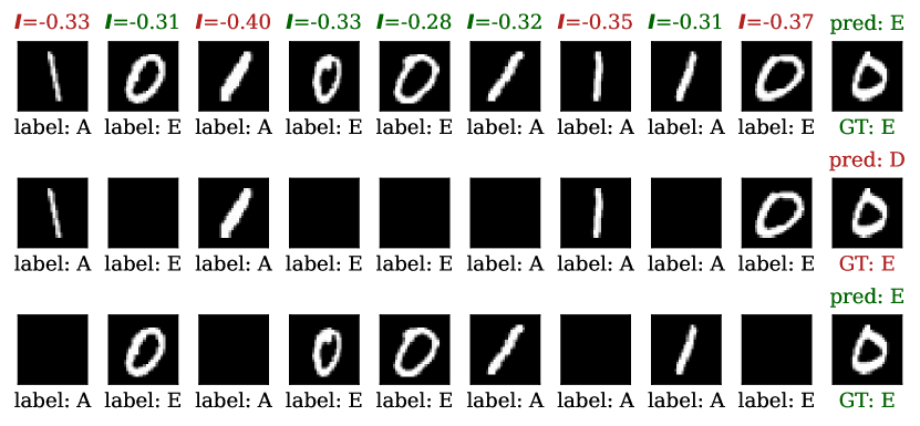
Figure 2: (Left) Visualization of learning label mapping of MNIST digits in context. The left $9$ images in each row are demonstrations while the right-most one is a query image. Below each image shows its mapped label (“A” to “E”). Above each ICL image is its $\mathcal{I}_{\text{test}}$ w.r.t. the query image with high values highlighted in green and low values highlighted in red. Above the query image is the prediction (pred) made by the pre-trained transformer which is in green if consistent with the ground truth (GT) and red otherwise. Top row shows that using all $9$ demonstrations allows the transformer to learn the mapping in context as GT$=$pred$=$“E”. Middle shows removing $5$ demonstrations with the highest $\mathcal{I}_{\text{test}}$ results in most digit $0$’s removed, leading to a wrong prediction. Bottom shows removing $5$ demonstrations with the lowest $\mathcal{I}_{\text{test}}$ results in $3$ digit $0$’s remaining for the transformer to learn in context, leading to correct prediction. (Right) Average accuracy on $1013$ ICL datasets repeated over $10$ trials; $\lambda=0.01$; Lines and shades represent mean and standard error over $10$ independent trials.

5.2 Evaluation on Large Language Models

With the insight obtained in Sec. 5.1, we now apply DETAIL to full-fledged LLMs. We start with demonstration perturbation and noisy demonstration detection to demonstrate that DETAIL can be used to interpret the quality of a demonstration. Then, leveraging these results, we further show how we can apply the DETAIL scores to tasks more closely related to real-world scenarios.

A distinction between LLMs and the custom transformer used above is that demonstrations in LLMs are usually a sequence of tokens, whereas demonstrations in the custom transformer are single tokens representing the actual numerical values of the problems (see Fig. 2). This distinction makes it difficult to find an appropriate internal representation for each demonstration (i.e., $m$). To overcome this challenge, we draw inspiration from prior works [49, 53] which suggest that information flows from input words to output labels in ICL. As an implementation detail, we take the embedding of the last token before the label token (hereafter referred to as the target position) in the middle layer where most of the information has flown to the target token positions. We include ablation studies on using different layers’ embeddings in Sec. D.6 and using different target positions in Sec. D.7.

Setup.

We consider (for white-box models) mainly a Vicuna-7b v1.3 [59] and also a Llama-2-13b [46] on some tasks using greedy decoding to show that DETAIL works on models with different training data and of varying sizes. While our theoretical backing stands for transformer-based models, we experiment DETAIL on Mamba-2.8b [23], a state-space model architecture that has received increased attention recently in Sec. D.8. We primarily evaluate our method on AG News ($4$ classes) [58], SST-2 ($2$ classes) [44], Rotten Tomatoes ($2$ classes) [40], and Subj ($2$ classes) [16] datasets which all admit classification tasks. Due to space limits, some results are deferred to App. D.

Demonstration perturbation.

We show that DETAIL can explain LLM predictions by showing how perturbation (i.e., corrupting the labels of some demonstrations to an incorrect class or removing some demonstrations) with the high/low $\mathcal{I}_{\text{test}}$ affects the model’s predictive power. We randomly pick $20$ ICL datasets each comprising $20$ demonstrations and $1$ query from AG News and find the average and standard error of the accuracy of predicting the query after perturbation using Vicuna-7b and Llama-2-13b, shown in Fig. 3 (results for other datasets deferred to Sec. D.1). It can be observed that perturbing demonstrations with low $\mathcal{I}_{\text{test}}$ results in a slower drop (or even improvement) in accuracy and vice versa, similar to the trend observed in Fig. 2, showcasing the applicability of DETAIL to LLMs. We additionally include the results using Falcon-7b [4] and Llama-2-7b [46] in Sec. D.1 where we perturb $10$ demonstrations and observe a similar accuracy gap.

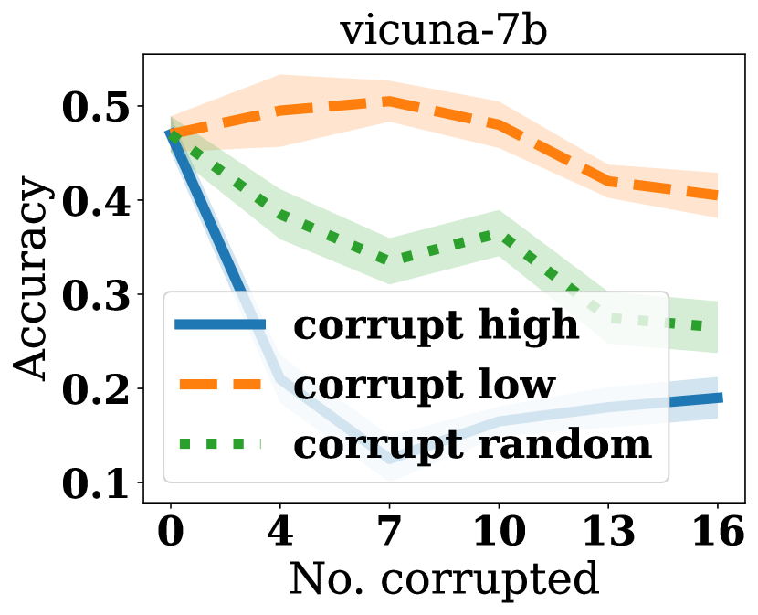
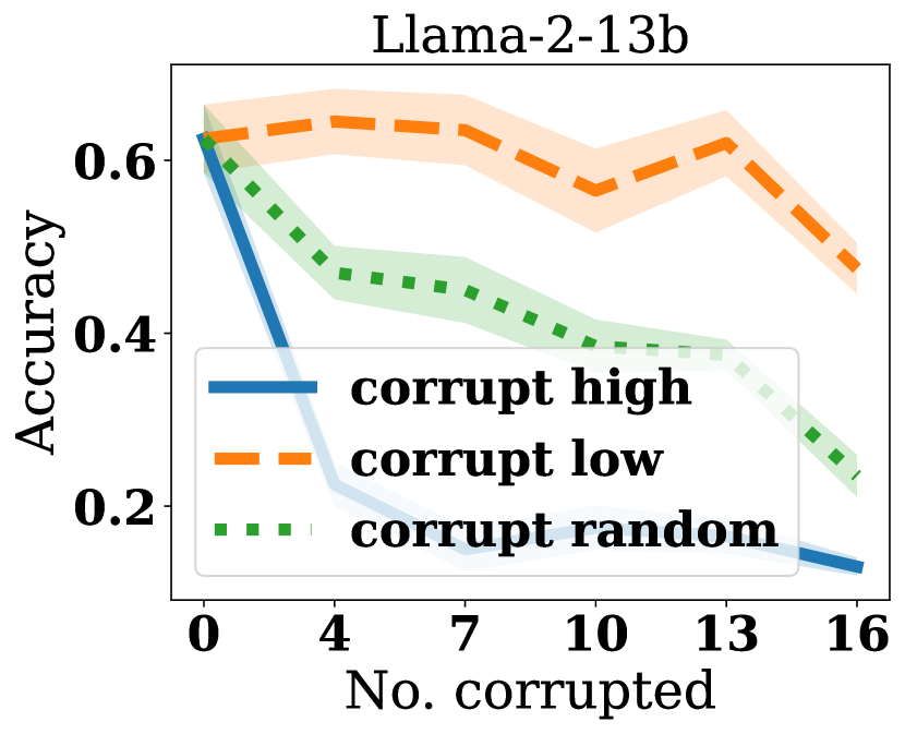
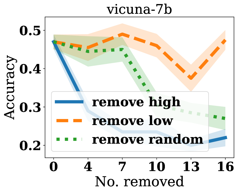
Figure 3: ($1$st and $2$nd) Corrupting labels of demonstrations and ($3$rd and $4$th) removing demonstrations with high/low DETAIL scores ($\mathcal{I}_{\text{test}}$) on AG News. Perturbing demonstrations randomly result in an accuracy in the middle as expected. All experiments are repeated $10$ trials. $\lambda=1.0$. Lines and shades represent the mean and standard error respectively.

Noisy demonstration detection.

We utilize the DETAIL score to detect noisy demonstrations with corrupted labels. The experiment setup largely follows [27, Section 5.4]. We randomly draw $100$ ICL datasets each consisting of $20$ demonstrations and $1$ query. For each ICL dataset, we randomly corrupt the labels of $4$ demonstrations (i.e., flipping the label to an incorrect class). The demonstrations are then ranked in descending order of their $\mathcal{I}_{\text{self}}$. The fraction of noisy demonstrations detected is plotted in the first $3$ figures of Fig. 4 (result for other datasets deferred to Sec. D.2). We compare our method with the leave-one-out (LOO) score [17] where the difference in cross-entropy loss of the model output is used as the utility. It can be observed that LOO performs close to random selection, whereas our method has a much higher identification rate w.r.t. the number of demonstrations checked. We also note that our method not only outperforms LOO in effectiveness but is also around $10\times$ faster than LOO since LOO requires multiple LLM inferences for each demonstration in the ICL dataset.

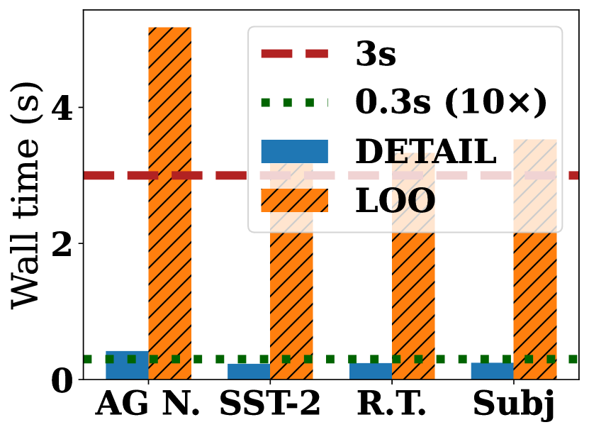
Figure 4: ($1$st and $2$nd) Fraction of noisy labels identified vs. number of demonstrations ranked by DETAIL (with $d^{\prime}=1000$) and LOO checked on Subj using Vicuna-7b and Llama-2-13b respectively. ($3$rd) Wall time comparison between DETAIL and LOO on all datasets. ($4$th) wall time in seconds (left $y$-axis) and AUCROC (right $y$-axis) vs. projection dimension on Subj using Vicuna-7b. All experiments are repeated $10$ trials. $\lambda=10^{-9}$. Lines and shades represent the mean and std. error.

Dimension reduction via random projection.

We analyze the impact of random projection on the effectiveness of DETAIL. Intuitively, dimension reduction trades off the effectiveness of DETAIL with computational efficiency, specifically the $\mathcal{O}(d^{3})$ cost for inverting $K_{\mathcal{I}}$. To understand the trade-off, we follow the same setup as the noisy demonstration detection experiment and compare the change in AUC ROC of detection and system wall time as the dimension $d^{\prime}$ of the projection matrix $P$ decreases. The result for Subj is in the last figure of Fig. 4 (results for other datasets deferred to Sec. D.3), showing that wall time stays minimal ($\approx 0.3$s) for project dimensions up to $1000$ generally before it exponentially increases. Effectiveness measured in terms of AUC reaches optimal with $d^{\prime}\geq 1000$. The results suggest a “sweet spot” –  $d^{\prime}\approx 1000$ –  for a low running time and high performance.

5.3 Applications of DETAIL

With the two experiments above verifying the effectiveness of DETAIL ($\mathcal{I}_{\text{self}}$ and $\mathcal{I}_{\text{test}}$) and the experiment on random projection which ensures computational efficiency, we demonstrate next how DETAIL, with $\mathcal{I}_{\text{self}}$ for noisy demonstration detection and $\mathcal{I}_{\text{test}}$ for demonstration perturbation, can be applied to real-world scenarios, achieving superior performance and speed.

ICL order optimization.

One distinctive trait of ICL compared to conventional ML is that the order of demonstrations affects the model’s predictive performance [32, 34]. We show that $\mathcal{I}_{\text{self}}$ helps reorder the demonstrations with improved model predictive performance. We first show, using a Vicuna-7b model, that moving demonstrations with lower quality to the front (or back) of the prompt tends to improve the test accuracy of the model. To see this, we corrupt the label of a random demonstration and allocate this corrupted demonstration to different positions of the ICL dataset (each with $20$ demonstrations with permutations drawn from a Sobol sequence [36] to capture the average performance better). A general trend with decreasing-then-increasing accuracy can be observed in Fig. 5: Allocating noisy demonstrations to the front (or the back) results in much higher test accuracy. Leveraging this insight, we utilize $\mathcal{I}_{\text{self}}$ to reorder a random permutation of ICL demonstrations and show the reordered prompt improves the test accuracy. For each randomly ordered prompt, $\mathcal{I}_{\text{self}}$ for each demonstration is computed (note that this computation only requires $1$ pass of the LLM). Then, based on the trend observed in Fig. 5, for Subj and Rotten Tomatoes datasets, the demonstrations are reordered by placing the two demonstrations with the largest $\mathcal{I}_{\text{self}}$ in front followed by the rest in ascending order. For SST-2, the demonstrations are reordered in descending order of $\mathcal{I}_{\text{self}}$. To simulate situations where demonstrations have varying quality, we additionally consider randomly perturbing $3$ demonstrations (and $6$ demonstrations in Sec. D.4) in each ICL dataset. We note a clear improvement in test accuracy of $1.4\%\sim 3.0\%$ via reordering demonstrations only, as shown in Sec. 5.3. The improvement demonstrates that $\mathcal{I}_{\text{self}}$ can identify demonstrations that are low-quality or inconsistent with other demonstrations in the ICL dataset.

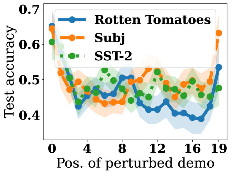
Figure 5: Test accuracy (mean and std. error) vs. position of the demonstration with the corrupted label over $50$ trials.

Table 1: Predictive accuracy of demonstrations permuted randomly and based on $\mathcal{I}_{\text{self}}$, respectively. The mean and standard error (in bracket) with $80$ repeated trials is shown.

	Subj	SST-2	Rotten Tomatoes
No corrupted demo
Baseline (random)	0.722 (7.22e-03)	0.665 (5.24e-03)	0.660 (1.08e-02)
Reorder (DETAIL)	0.743 (7.10e-03)	0.679 (5.42e-03)	0.684 (1.15e-02)
Difference $\uparrow$	0.0206 (7.40e-03)	0.0139 (6.08e-03)	0.0244 (1.11e-02)
Corrupt $3$ demos
Baseline (random)	0.655 (8.54e-03)	0.607 (7.61e-03)	0.553 (1.10e-02)
Reorder (DETAIL)	0.685 (9.39e-03)	0.630 (7.04e-03)	0.582 (1.42e-02)
Difference $\uparrow$	0.0300 (9.10e-03)	0.0230 (7.22e-03)	0.0291 (1.06e-02)

ICL demonstration curation.

In the demonstration perturbation experiment, we have verified that our $\mathcal{I}_{\text{test}}$ can correctly attribute helpful demonstrations w.r.t. a query. A direct application is demonstration curation where a subset of most helpful demonstrations are selected to prompt the LLM while maintaining accuracy on a test dataset. This application is useful, especially for saving the cost of querying LLMs. For proprietary LLMs, reducing the prompt length can also significantly save inference time which scales quadratically in the prompt length. As a setup, we fix a randomly selected set of $120$ demonstrations as the test set. In each trial, we randomly pick $20$ demonstrations to form an ICL dataset and another $20$ demonstrations as the validation set. The individual $\mathcal{I}_{\text{test}}$’s on each validation demonstration are summed as the final score. Then, demonstrations with the lowest scores are removed (in position). We randomly corrupt $5$ demonstrations in each ICL dataset to simulate prompts with varying qualities. The results are shown in Fig. 6 (results on other datasets deferred to Sec. D.5). A clear gap between the test accuracy after removing demonstrations with high/low $\mathcal{I}_{\text{test}}$ can be observed for both Vicuna-7b and Llama-2-13 on both binary (Rotten Tomatoes) and $4$-way classification (AG News). Removing demonstrations with lower $\mathcal{I}_{\text{test}}$’s maintains (or even improves) the test accuracy. Moreover, the gap for the 13B model is wider and more certain (shorter error bars), signaling better curation. We attribute this phenomenon to the better capability of the larger model to formulate an “internal optimizer”, which enhances the attributive power of $\mathcal{I}_{\text{test}}$.

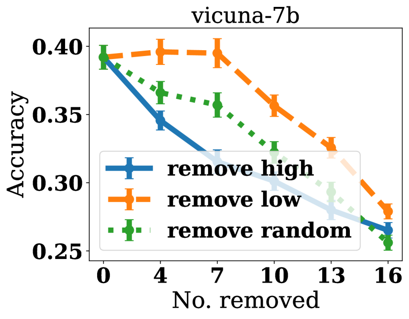
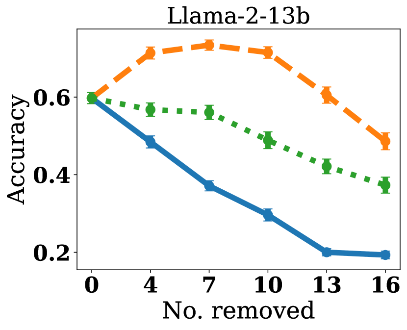
Figure 6: Test accuracy vs. number of demonstrations removed using $\mathcal{I}_{\text{test}}$ on ($1$st and $2$nd) AG news and ($3$rd and $4$th) Rotten Tomatoes using Vicuna-7b and Llama-2-13b. All experiments are repeated with $80$ trials. Lines and bars represent the mean and standard error.

5.4 Comparison with Other Attribution Methods

We compare our DETAIL score with other metrics proposed for demonstration attribution/selection or can be directly extended to attributing demonstrations. We analyze both the attributability via a demonstration curation experiment and the computational cost via recording the system wall time for performing the attribution. We select representative conventional approaches from different paradigms, including integrated gradients (IG) [45] and LIME [41] (Attention [6] in Sec. D.5). As these methods are originally designed for token-level attribution, we use the sum of the scores of all tokens in each demonstration as the attribution score. We also compare recent efforts on demonstration selection [13, 38, 42]. We select an ICL dataset of $20$ demonstrations, compute the attribution scores on a validation set of $20$ demonstrations, and record the accuracy after removing $10$ demonstrations in place on $120$ test queries. The results are tabulated in Table 2. For hyper-parameter, we choose $M=100$ and $k=1$ for [38], $5$ iterations of LiSSA update [1] for [42], and $M=10,K=4$ for datamodel [13]. We do not perform batch inference for a fair comparison of computational time as some approaches do not admit batch inference. We also use a projection of $d^{\prime}=1000$ to compute $\mathcal{I}_{\text{test}}$. It can be observed that DETAIL outperforms all other attribution methods in test accuracy. Our computation is efficient (with wall time of $4\sim 10$s), achieving over $5\times$ speedup compared to other methods except [42] which achieves a comparable computational time to ours but a lower accuracy. Notably, IG and LIME perform close to random removal, which is likely because these methods are designed for token-level attribution and generalize poorly to demonstration-level attribution.

Table 2: Test accuracy after curating the ICL dataset and the incurred wall time (in seconds on one L40 GPU). The mean and std. error (in bracket) is shown with $20$ repeated trials.

Metric	DETAIL ($d^{\prime}=1000$)	IG [45]	LIME [41]	[38]	[42]	Datamodel [13]	Random
Subj
Accuracy $\uparrow$	0.747 (2.60e-02)	0.658 (2.22e-02)	0.665 (2.41e-02)	0.583 (2.75e-02)	0.556 (1.38e-02)	0.658 (2.62e-02)	0.654 (2.54e-02)
Wall time $\downarrow$	5.22 (1.17e-01)	593 (1.20e+01)	393 (2.44e+01)	54.3 (3.78e-01)	9.37 (4.19e-01)	746 (3.42e+00)	N.A.
SST-2
Accuracy $\uparrow$	0.607 (2.12e-02)	0.458 (2.06e-02)	0.476 (1.87e-02)	0.513 (1.88e-02)	0.493 (1.34e-02)	0.460 (2.36e-02)	0.469 (2.15e-02)
Wall time $\downarrow$	4.88 (1.35e-01)	458 (7.99e+00)	337 (1.69e+01)	121 (4.79e+00)	10.6 (7.80e-01)	713 (1.96e+00)	N.A.
Rotten Tomatoes
Accuracy $\uparrow$	0.555 (1.94e-02)	0.442 (2.13e-02)	0.435 (1.39e-02)	0.520 (2.17e-02)	0.498 (1.72e-02)	0.484 (1.87e-02)	0.457 (2.19e-02)
Wall time $\downarrow$	5.11 (1.06e-01)	525 (1.23e+01)	245 (6.32e+01)	122 (4.68e+00)	9.74 (5.57e-01)	732 (2.10e+00)	N.A.
AG News
Accuracy $\uparrow$	0.412 (1.35e-02)	0.351 (1.65e-02)	0.368 (1.73e-02)	0.392 (1.42e-02)	0.361 (1.83e-02)	0.373 (1.31e-02)	0.379 (1.70e-02)
Wall time $\downarrow$	10.4 (1.07e-01)	1208 (2.16e+01)	599 (1.03e+01)	81.3 (6.05e-01)	6.94 (4.78e-02)	997 (7.55e+00)	N.A.

5.5 Transferability to Black-box Models

We evaluate the transferability of DETAIL on GPT-3.5, a popular black-box model. We experiment with both the demonstration reordering and demonstration curation tasks where we compute the DETAIL scores on a Vicuna-7b model (white-box) and then test the performance on GPT. Our method produces promising results on both tasks as shown in Sec. 5.5 and Sec. 5.5 respectively. Notably, curating demonstrations with our method achieves a $17.9\%$ average improvement in accuracy compared to random curating on the demonstration curation task (Sec. 5.5). We also note an over $2\%$ improvement in accuracy for reordering task if we corrupt $3$ demonstrations (Sec. 5.5). With no corrupted demonstration, reordering with our approach does not improve performance on GPT-3.5, which we attribute to the stronger inference power of GPT-3.5, resulting in less variance w.r.t. demonstration orders, consistent with the findings in [34].

Table 3: Accuracy (on GPT-3.5) of demonstrations (demos) permuted randomly and based on $\mathcal{I}_{\text{self}}$. Mean and std. error (in bracket) with $80$ trials is shown.

	Subj	SST-2	Rotten Tomatoes
No corrupted demo
Baseline (random)	0.708(7.79e-04)	0.799(7.52e-04)	0.901(6.01e-04)
Reorder (DETAIL)	0.711(7.51e-04)	0.792(9.01e-04)	0.909(4.84e-04)
Difference $\uparrow$	0.002(7.52e-04)	-0.007(6.49e-04)	0.008(6.14e-04)
Corrupt $3$ demos
Baseline (random)	0.628(8.21e-04)	0.720(1.11e-03)	0.788(1.44e-03)
Reorder (DETAIL)	0.660(9.57e-04)	0.742(1.20e-03)	0.816(1.60e-03)
Difference $\uparrow$	0.032(8.61e-04)	0.022(8.92e-04)	0.028(1.10e-03)

Table 4: Accuracy (on GPT-3.5) on a test dataset of size $20$ after curating $10$ demonstrations from the ICL dataset. The mean and std. error (in bracket) of accuracy after removal is shown with $20$ repeated trials.

Dataset	DETAIL ($d^{\prime}=1000$)	Random
Subj	0.842 (2.16e-02)	0.660 (3.47e-02)
SST-2	0.812 (1.96e-02)	0.618 (5.51e-02)
Rotten Tomatoes	0.690 (4.66e-02)	0.420 (5.14e-02)
AG News	0.515 (3.08e-02)	0.447 (2.73e-02)

6 Conclusion, Limitation, and Future Work

We tackle the problem of attributing demonstrations in ICL for transformers. Based on the well-known influence function commonly used for attributing conventional ML, we propose DETAIL, an innovative adoption of the influence function to ICL through the lens of treating the transformer as implementing an internal kernelized ridge regression. Combined with a dimension reduction technique using random projection, DETAIL can be computed in real-time with an impressive performance on various real-world related tasks such as demonstration order optimization and demonstration curation. One limitation of our approach is the need to access the internal state of the transformer, which we mitigate by additionally showing that DETAIL scores are transferable to black-box models. As a first step toward attributing demonstrations w.r.t. a transformer’s internal optimizer, we hope this work serves as a building block for future research to develop attribution techniques for more generalized in-context learning settings such as chain-of-thought [50].

Appendix A Computational Resources

Hardware.

All our experiments about 7B white-box models are conducted on a single L40 GPU. All experiments involving 13B white-box models are conducted on a single H100 GPU. Total budget for GPT-3.5 API calls to conduct the transferability experiments in Sec. 5.5 is estimated to be around US$500 (at the rate of US$0.5/1mln tokens for input and US$1.50/1mln tokens for output).

Software.

All our experiments are conducted using Python3.10 on a Ubuntu 22.04.4 LTS distribution. We use Jax [11] for the experiments in Sec. 5.1 and use PyTorch 2.1.0 [5] for the experiments in Sec. 5.2 and Sec. 5.3. We adopt the implementations of the LLMs (transformer-based and SSM-based) provided in the Huggingface’s “transformers” [51] system throughout this work. The NLP datasets are also obtained from Huggingface’s “datasets” API [29]. The precise repository references and other dependencies can be found in the code provided in the supplemental materials.

Appendix B Algorithmic Implementation

We provide an implementation of computing our DETAIL score for LLM in Alg. 1. Line 6 shows the (optional) random projection where a random matrix $P$ is multiplied by the embeddings. In line 8, $\beta$ has a closed-form expression as the solution to a regularized ridge regression. In line 10 and line 14, we select the embeddings of the target positions. Then, depending on whether we use self-influence, we use different embeddings for computing $\nabla_{\beta}L$ as shown in lines 15-19. Line 20 computes the inverse hessian $H_{\beta}^{-1}=(K_{\mathcal{I}}+\lambda I)^{-1}$ before finally calculating $\mathcal{I}_{i}$ in line 21.

Algorithm 1 DETAIL

1:Input: model $M$, prompt tokens $x_{[1:n]}$, label tokens $y_{[1:t]}$, target positions $p_{[1:t]}$, total number of transformer layers $L$, transformer layer to compute DETAIL score $l$, regularization constant $\lambda$, projection matrix $P\in\mathbb{R}^{d\times d^{\prime}}$ (default $I$)

2:$\mathcal{I}_{i}\leftarrow 0$ for $i\in\{1,2,\cdots,t-1\}$

3:$h_{1},h_{2},\cdots,h_{L}\leftarrow M(x_{[1:n]})$

4:$p_{\text{demo}}\leftarrow p_{[1:t-1]}$ $\triangleright$ Remove the last target which is the test query

5:$y_{\text{demo}}\leftarrow\text{one\_hot}(y_{[1:t-1]})$ $\triangleright$ Remove the last label and convert to one-hot

6:$m_{\text{demo}}\leftarrow h_{l}[p_{\text{demo}}]P$ $\triangleright$ Optional dimensionality reduction

7:$K_{\beta}\leftarrow m_{\text{demo}}m_{\text{demo}}^{\top}$ $\triangleright$ $K_{\beta}\in\mathbb{R}^{(t-1)\times(t-1)}$ for speed-up as $t\ll d^{\prime}$

8:$\beta\leftarrow[(K_{\beta}+\lambda{I})^{-1}m_{\text{demo}}]^{\top}y_{\text{demo}}$

9:$p_{\text{test}}\leftarrow p_{[t-1:t]}$

10:$m_{\text{test}}\leftarrow h_{l}[p_{\text{test}}]$

11:$y_{\text{test}}\leftarrow\text{one\_hot}(y_{[t-1:t]})$

12:$K_{\mathcal{I}}\leftarrow m_{\text{demo}}^{\top}m_{\text{demo}}$ $\triangleright$ $K_{\mathcal{I}}\in\mathbb{R}^{d^{\prime}\times d^{\prime}}$

13:for $i\in\{1,2,\cdots,t-1\}$ do

14:     $m_{i}\leftarrow h_{l}[p_{[i:i+1]}]P$

15:     if self influence then

16:         $\nabla_{\beta}L\leftarrow m_{i}^{\top}(m_{i}\beta-y_{\text{demo}}[i])+\lambda\beta$

17:     else if 

18:          then$\nabla_{\beta}L\leftarrow m_{\text{test}}^{\top}(m_{\text{test}}\beta-y_{\text{test}})+\lambda\beta$

19:     end if

20:     $\mathcal{I}_{\text{reg}}\leftarrow(K_{\mathcal{I}}+\lambda{I})^{-1}[m_{i}^{\top}(m_{i}\beta-y_{\text{demo}}[i])+\lambda\beta]$ $\triangleright$ Eq. 5 with the constant dropped

21:     $\mathcal{I}_{i}\leftarrow\mathcal{I}_{i}+(\nabla_{\beta}L)^{\top}\mathcal{I}_{\text{reg}}$ $\triangleright$ Eq. 6

22:end for

23:Return $\mathcal{I}$

Appendix C Additional Discussion

Potential societal impact.

We propose an attribution technique for improving the interpretability of in-context learning. We believe our research has potential positive societal impacts in improving the safety of LLMs via filtering out corrupted/harmful demonstrations as demonstrated by our experiments as well as saving energy by curating the demonstration, hence reducing the cost of querying LLMs. We do not find any direct negative societal impact posed by our research contribution.

Setting $\lambda$.

Generally, there is no golden rule for the most appropriate $\lambda$ that regularizes the ridge parameters $\beta$. Intuitively, a larger $\lambda$ likely works better when the dimension of $\beta$ is large since the model tends to be over-parameterized (i.e., in a LLM). Therefore, we set a relatively large $\lambda=1.0$ for LLMs and a relatively small $\lambda=0.01$ for our custom transformer. When detecting noisy demonstrations, we may not want to regularize $\beta$ too much because we wish to retain the information captured by the eigenvalues of the hessian $H$ which can be eroded with a larger $\lambda$. As such, for the noisy demonstration detection task, we set a very small $\lambda=10^{-9}$ to retain most of the information captured by $H$ while ensuring that it is invertible.

Random projection matrix.

We recall the Johnson-Lindenstrauss (JL) lemma [18, 26].

Theorem C.1 (Johnson-Lindenstrauss Lemma).

For any $0<\epsilon<1$ and any integer $n$, let $d^{\prime}$ be a positive integer such that

$$d^{\prime}\geq\frac{24}{3\epsilon^{2}-2\epsilon^{3}}\log{n}\ ,$$

then for any set $A$ of $n$ points $\in\mathbb{R}^{d}$, there exists a mapping $f:\mathbb{R}^{d}\to\mathbb{R}^{d^{\prime}}$ such that for all $x_{i},x_{j}\in A$,

$$(1-\epsilon)\|x_{i}-x_{j}\|^{2}\leq\|f(x_{i})-f(x_{j})\|^{2}\leq(1+\epsilon)\|x_{i}-x_{j}\|^{2}\ .$$

A specific constructive proof is by setting $A\coloneqq\frac{1}{\sqrt{d^{\prime}}}R$ where $R_{i,j}\overset{\text{i.i.d.}}{\sim}\mathcal{N}(0,1)$. In our work, we treat each embedding $m$ as $x$ and the projected embedding $mP$ as $f(x)$. The specific construction follows the abovementioned constructive proof defining

$$P\coloneqq\frac{1}{\sqrt{d^{\prime}}}R\sim\mathcal{N}(\boldsymbol{0},\frac{1}{d^{\prime}}\boldsymbol{I})\ .$$

Empirically, our threshold $d^{\prime}=1000$ corresponds to $\epsilon\lessapprox 0.164$, ensuring a good preservation of (Euclidean) distance between points.

ICL prompt example.

We include a visualization of a prompt for ICL below. Each input-output pair consists of a task demonstration. The query is appended at the end of the prompt with only the input and the output header.

Appendix D Additional Experiments

D.1 Additional Results for Demonstration Perturbation Task

We include the full results for the demonstration perturbation task using a Vicuna-7b v1.3 model in Fig. 7 and using a Llama-2-13b model in Fig. 8. A consistent trend can be observed across different datasets using both models.

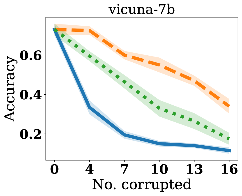
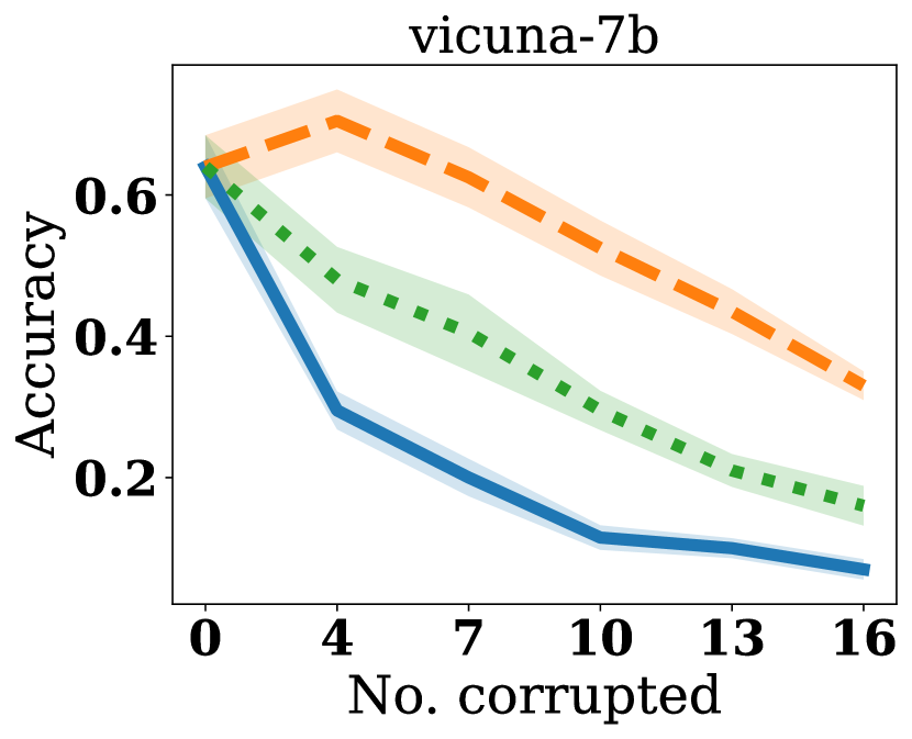
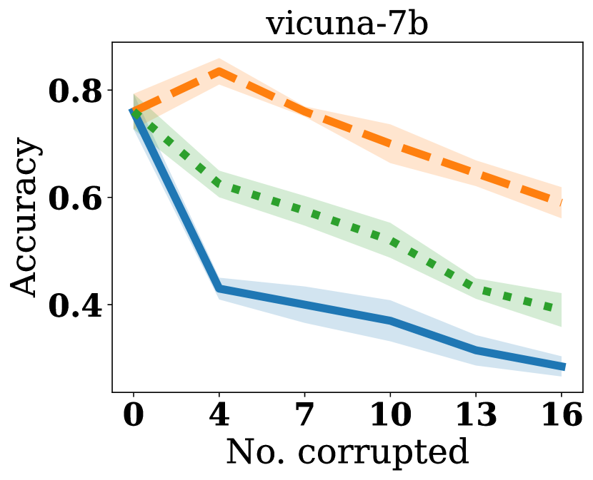
Figure 7: Corrupting and removing demonstration on datasets affects the model predictive power differently on AG News and SST-2, Rotten Tomatoes, and Subj from left to right using Vicuna-7b. Corrupting/removing demonstrations with high DETAIL scores results in lower model accuracy and vice versa. Corrupting/removing demonstrations randomly results in an accuracy in the middle as expected. All experiments are repeated with $10$ independent trials. $\lambda=1.0$. Lines and shades represent the mean and standard error respectively.

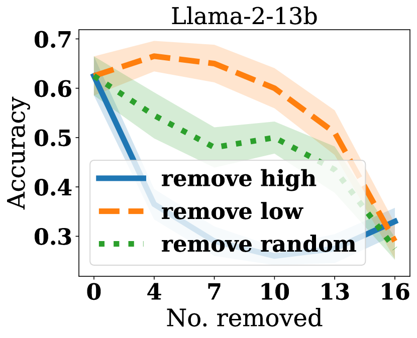
(a) AG News Removal

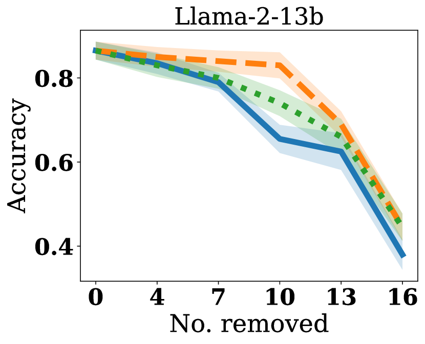
(b) SST-2 Removal

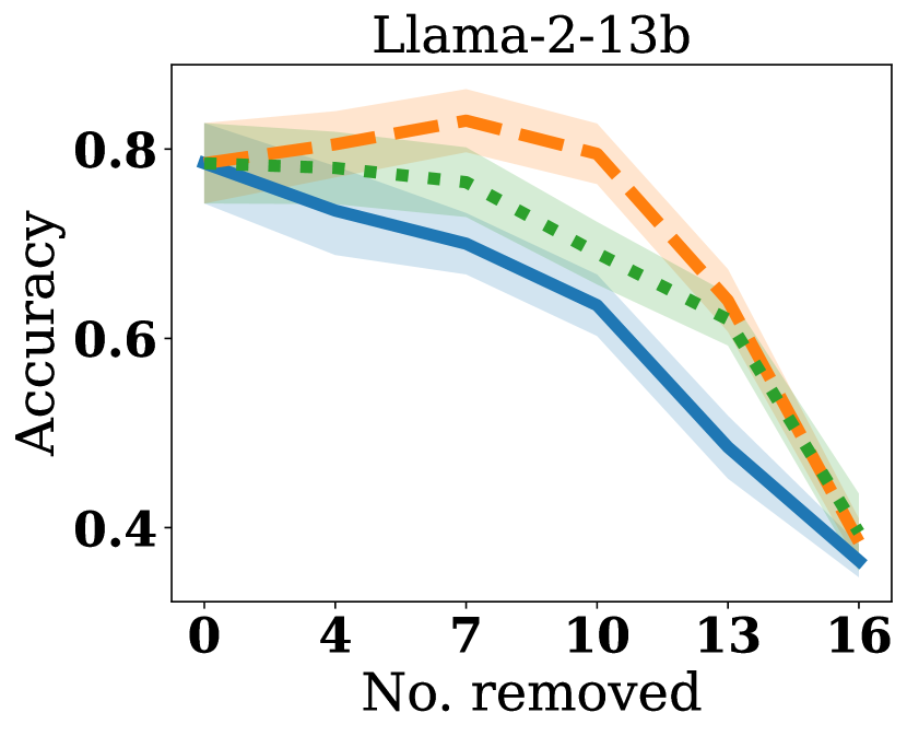
(c) Rotten Tomatoes Removal

(d) Subj Removal

(e) AG News Corrupt

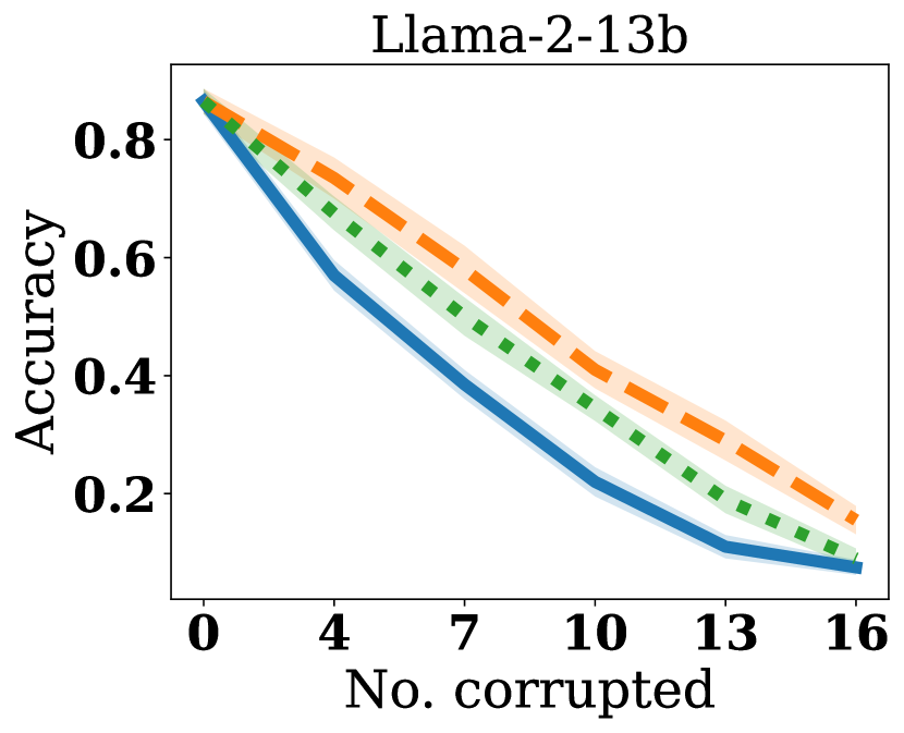
(f) SST-2 Corrupt

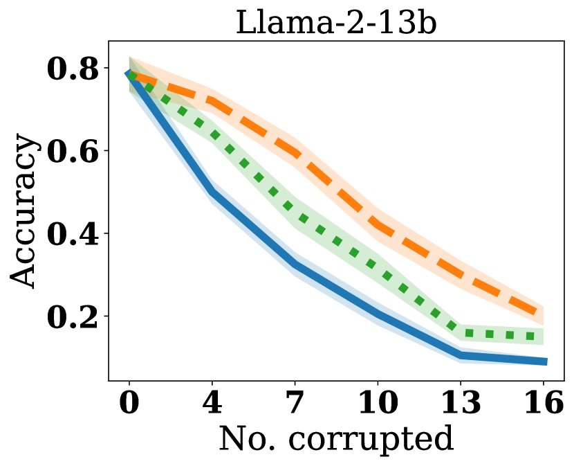
(g) Rotten Tomatoes Corrupt

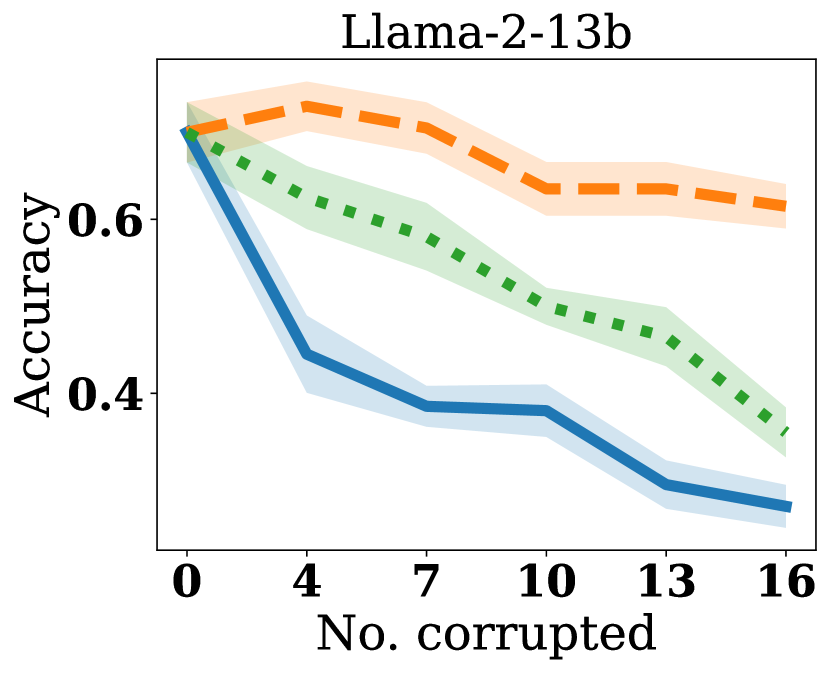
(h) Subj Corrupt

Figure 8: Results of model prediction accuracy vs. number of demonstrations removed/corrupted on Llama-2-13b model. $\lambda=1.0$. Lines and shades represent the mean and standard error respectively.

We compare (in addition to Vicuna-7b) a total of $3$ LLMs: Llama-2-7b [46], Llama-2-13b [46] and Falcon-7b [4]. We reuse the same experimental setup as the demonstration label perturbation task and compare the accuracy by removing and corrupting $10$ among $20$ ICL data with high/low DETAIL scores computed in different models. The results are tabulated in Table 5. A similar trend can be observed across these models where removing/corrupting demonstrations with high $\mathcal{I}_{\text{test}}$ results in lower accuracy and vice versa. The results demonstrate that our method is robust against model pre-training/fine-tuning data as well as model size.

Table 5: Performance on demonstration perturbation task across different models. The mean and standard error (in bracket) of predictive accuracy after removal or corruption $10$ out of $20$ demonstrations of $20$ randomly drawn ICL datasets is shown. All experiments are independently repeated $20$ times.

	remove high $\downarrow$	remove low $\uparrow$	remove random	corrupt high $\downarrow$	corrupt low $\uparrow$	corrupt random
Subj
Llama-2-7b	0.380 (0.034)	0.675 (0.025)	0.535 (0.035)	0.250 (0.036)	0.690 (0.031)	0.445 (0.019)
Llama-2-13b	0.570 (0.029)	0.700 (0.032)	0.575 (0.038)	0.380 (0.030)	0.635 (0.031)	0.500 (0.021)
Falcon-7b	0.450 (0.026)	0.690 (0.028)	0.580 (0.042)	0.280 (0.026)	0.630 (0.023)	0.445 (0.043)
SST-2
Llama-2-7b	0.480 (0.031)	0.670 (0.030)	0.540 (0.042)	0.145 (0.018)	0.445 (0.042)	0.275 (0.039)
Llama-2-13b	0.655 (0.034)	0.830 (0.031)	0.740 (0.031)	0.220 (0.025)	0.410 (0.031)	0.345 (0.022)
Falcon-7b	0.560 (0.043)	0.775 (0.028)	0.680 (0.032)	0.225 (0.031)	0.545 (0.030)	0.340 (0.023)
Rotten toamtoes
Llama-2-7b	0.435 (0.034)	0.670 (0.060)	0.540 (0.045)	0.120 (0.025)	0.420 (0.039)	0.235 (0.026)
Llama-2-13b	0.635 (0.032)	0.795 (0.032)	0.690 (0.033)	0.205 (0.028)	0.420 (0.040)	0.315 (0.035)
Falcon-7b	0.475 (0.037)	0.780 (0.024)	0.620 (0.024)	0.225 (0.023)	0.590 (0.031)	0.445 (0.025)
AG News
Llama-2-7b	0.145 (0.018)	0.525 (0.036)	0.360 (0.026)	0.150 (0.016)	0.520 (0.030)	0.325 (0.037)
Llama-2-13b	0.260 (0.018)	0.600 (0.041)	0.500 (0.032)	0.175 (0.026)	0.565 (0.049)	0.385 (0.031)
Falcon-7b	0.155 (0.019)	0.460 (0.021)	0.335 (0.025)	0.085 (0.020)	0.465 (0.017)	0.265 (0.027)

D.2 Additional Results for Noisy Demonstration Detection

We include the results on AG News, SST-2, Rotten Tomatoes, and Subj datasets using a Vicuna-7b model in Fig. 9. Similar trends as in the main text is observed. A counterpart experiment using Llama-2-13b is in Fig. 10, where a similar trend is observed.

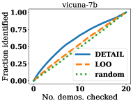
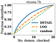
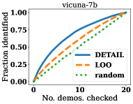
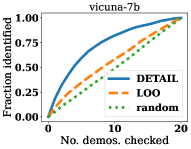
Figure 9: (Left to right) Fraction of all noisy labels identified vs. the number of demonstrations ranked by our method (with projection down to $1000$ dimension) and LOO checked respectively on AG News, SST-2, Rotten Tomatoes, and Subj datasets. $\lambda=10^{-9}$. All experiments are repeated with $10$ independent trials. Lines and shades represent the mean and standard error respectively.

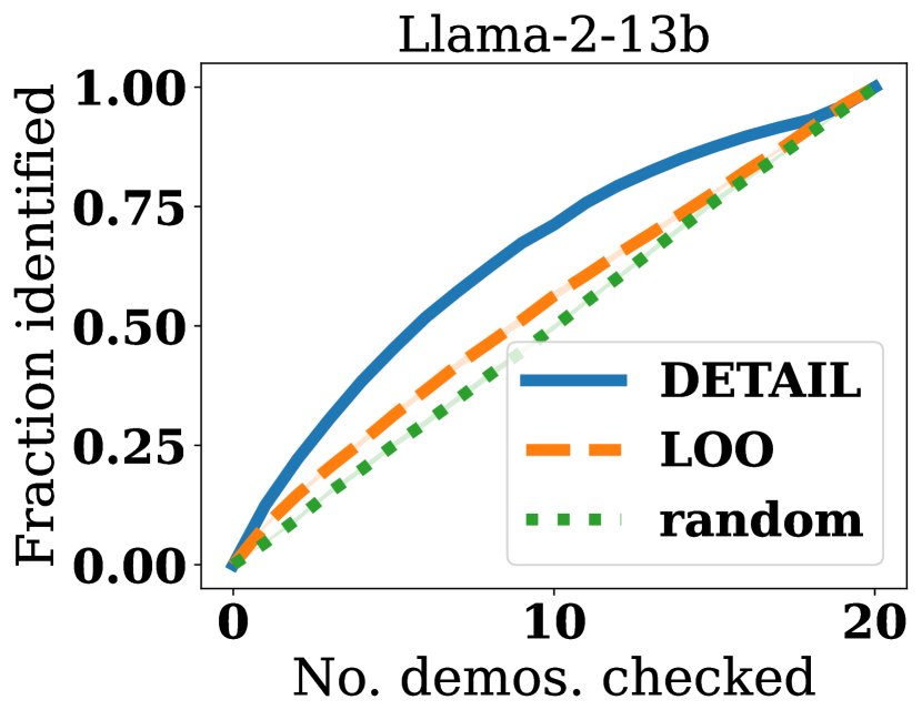
(a) Detecting noisy label on AG News

(b) Detecting noisy label on SST-2

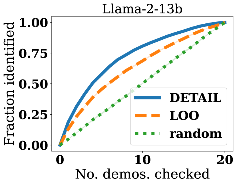
(c) Detecting noisy label on Rotten Tomatoes

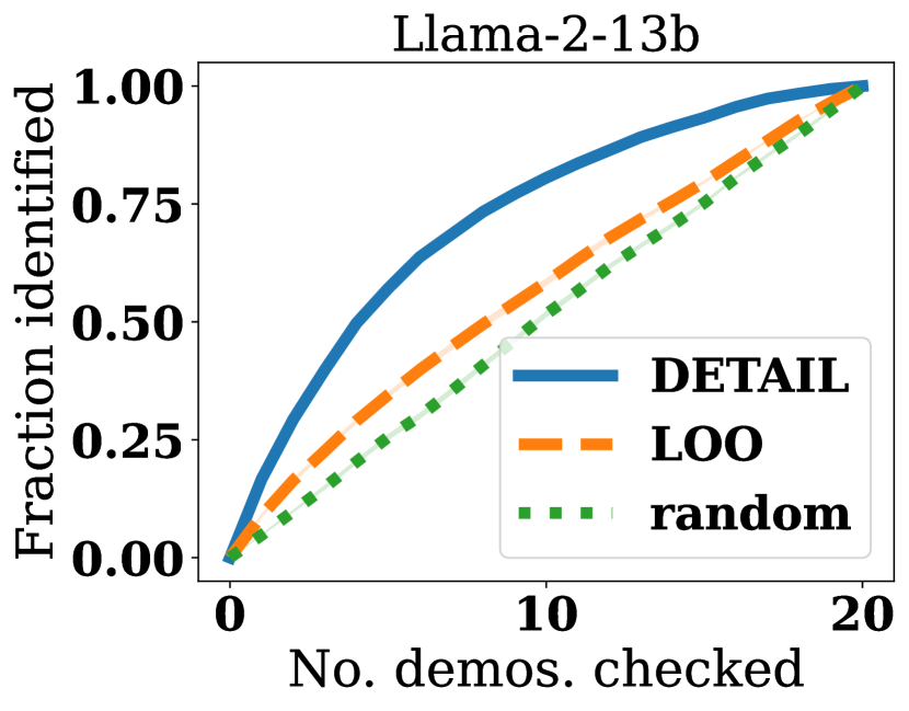
(d) Detecting noisy label on Subj

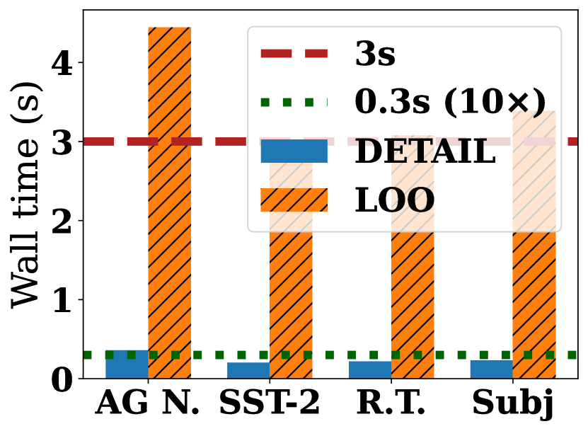
(e) Wall time comparison

Figure 10: (a-d) Fraction of all noisy labels identified vs. the number of demonstrations ranked by our method (with projection down to $1000$ dimension) and LOO checked respectively. (e) Wall time comparison across all datasets. $\lambda=10^{-9}$. All experiments are repeated with $10$ independent trials using a Llama-2-13b model. Lines and shades represent the mean and standard error respectively.

D.3 Additional Results for Dimension Reduction

The experiments using Vicuna-7b on AG News, SST-2, Rotten Tomatoes, and Subj can be found in Fig. 11. It can be observed that the trend is consistent across different datasets.

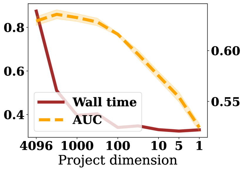
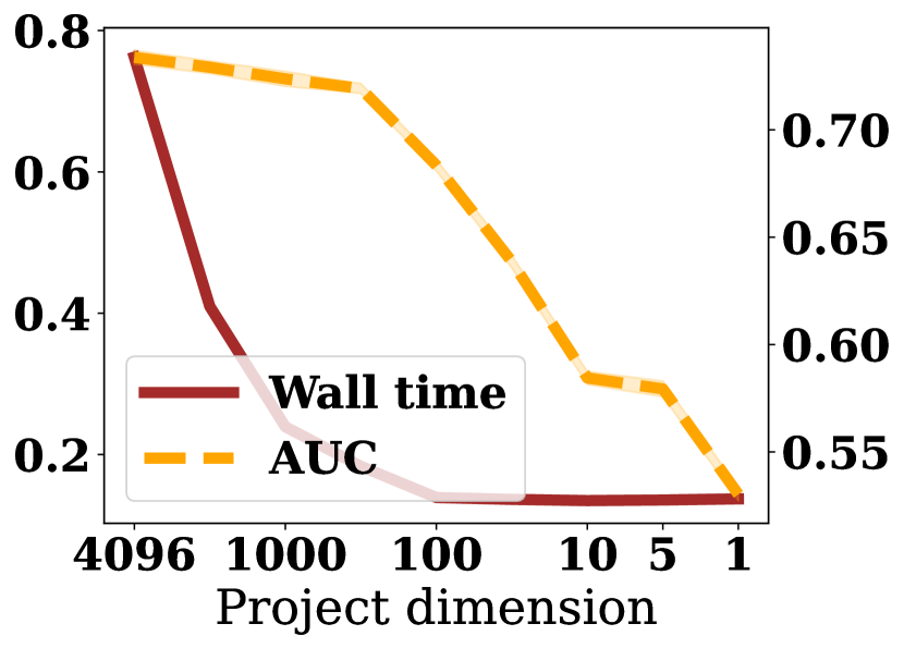
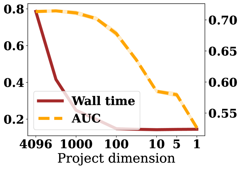
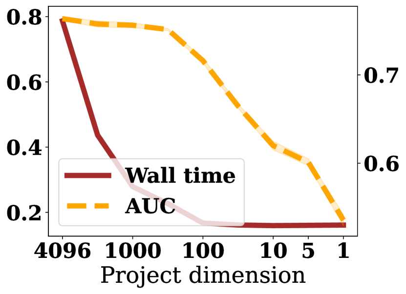
Figure 11: (Left to right) wall time in seconds (left $y$-axis) and AUCROC (right $y$-axis) vs. projection dimension $d^{\prime}$ on AG news, SST-2, Rotten Tomatoes, and Subj datasets. Experiments are repeated with $10$ trials. Lines and shades represent the mean and standard error respectively.

D.4 Additional Results for Demonstration Reordering Task

We conduct additional experiments on the demonstration reordering task by perturbing $6$ demonstrations in each ICL dataset of $20$ demonstrations. The results are shown in Sec. D.4. It can be observed that reordering with $\mathcal{I}_{\text{self}}$ still achieves an improvement in test accuracy, demonstrating the robustness of our method.

Table 6: Predictive accuracy of demonstrations permuted randomly and based on $\mathcal{I}_{\text{self}}$ respectively. The mean and standard error (in bracket) with $80$ repeated trials is shown.

	Subj	SST-2	Rotten Tomatoes
Corrupt $6$ demonstrations
Baseline (random)	0.588 (7.96e-03)	0.487 (9.45e-03)	0.398 (1.12e-02)
Reorder (DETAIL)	0.604 (7.39e-03)	0.520 (1.01e-02)	0.425 (1.37-02)
Difference $\uparrow$	0.0164 (7.05e-03)	0.0323 (8.13e-03)	0.0267 (1.01e-02)

D.5 Additional Results for Demonstration Curation Task

We include the full results for all datasets on both Vicuna-7b and Llama-2-13b in Fig. 12. It can be observed that the gap between removing demonstrations with high/low $\mathcal{I}_{\text{test}}$ is wider with Llama-2-13b. We believe this is because Llama-2-13b being a larger model possesses better capability of formulating the internal optimizer as compared to Vicuna-7b which is smaller.

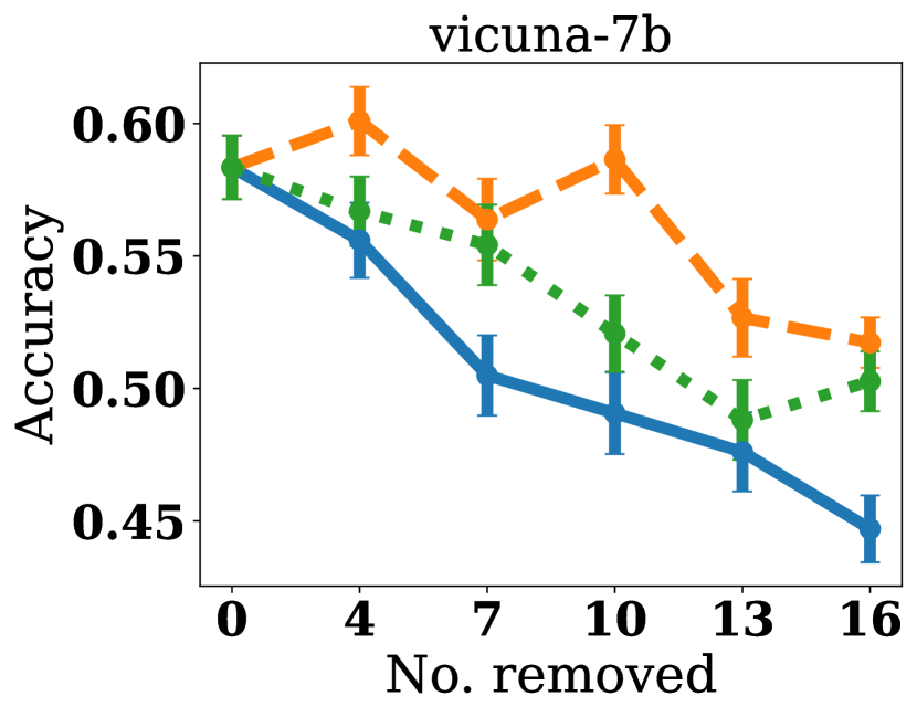
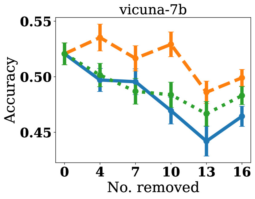
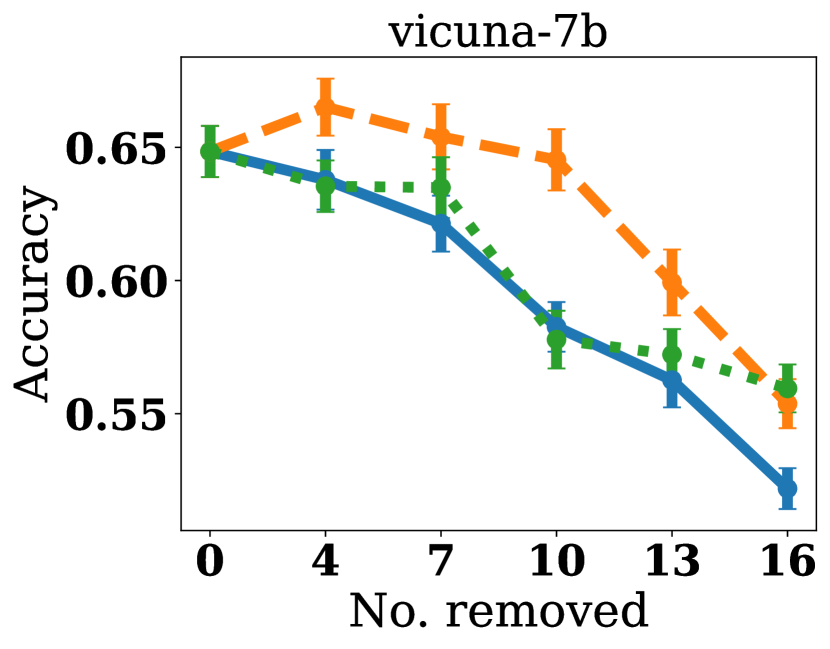
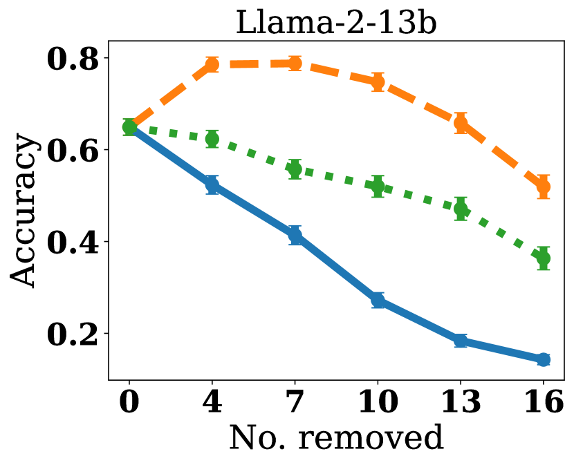
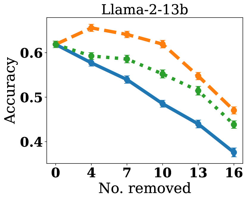
Figure 12: (Left to right) test accuracy vs. number of demonstrations removed using $\mathcal{I}_{\text{test}}$ on AG news, SST-2, Rotten Tomatoes, and Subj datasets using (top) Vicuna-7b and (bottom) Llama-2-13b. All experiments are repeated with $80$ independent trials. Lines and bars represent the mean and standard error respectively.

We additionally provide the result for the demonstration curation task with Attention [6] and [42] using $10$ iterations of LiSSA update for computing the hessian vector product [1] and compare it with the case with $5$ iterations. The result is shown in Table 7. With $10$ iterations, the wall time is much higher (over $20\times$) but accuracy is comparable to the case with $5$ iterations. For Attention, the performance is comparable to random removal as shown in Table 2.

Table 7: Test accuracy after curating the ICL dataset and the incurred wall time (in seconds on one L40 GPU). The mean and std. error (in bracket) is shown with $20$ repeated trials.

Metric	Attention [6]	[42] (#5)	[42] (#10)
Subj (curate $10$ demonstrations)
Accuracy $\uparrow$	0.627 (2.01e-02)	0.556 (1.38e-02)	0.597 (3.23e-02)
Wall time $\downarrow$	37.6 (1.09e+00)	9.37 (4.19e-01)	245 (8.80e-01)
SST-2 (curate $10$ demonstrations)
Accuracy $\uparrow$	0.460 (2.60e-02)	0.493 (1.34e-02)	0.499 (1.64e-02)
Wall time $\downarrow$	24.9 (7.26e-01)	10.6 (7.80e-01)	241 (9.63e-01)
Rotten Tomatoes (curate $10$ demonstrations)
Accuracy $\uparrow$	0.488 (2.05e-02)	0.498 (1.72e-02)	0.494 (1.74e-02)
Wall time $\downarrow$	36.8 (1.09e+00)	9.74 (5.57e-01)	240 (4.61e-01)
AG News (curate $10$ demonstrations)
Accuracy $\uparrow$	0.350 (1.35e-02)	0.416 (2.10e-02)	0.346 (2.07e-02)
Wall time $\downarrow$	138 (3.28e+00)	11.9 (5.78e-01)	441 (4.0e-01)

D.6 Ablation of Different Transformer Layers for Computing DETAIL scores.

We experiment with the difference in the effectiveness DETAIL using the embeddings of different layers. We conduct experiments on demonstration removal, demonstration perturbation, and noisy label detection tasks. The results are shown in Fig. 13. It can be observed that obtaining the DETAIL scores from the later layers of the model consistently produces desirable results.

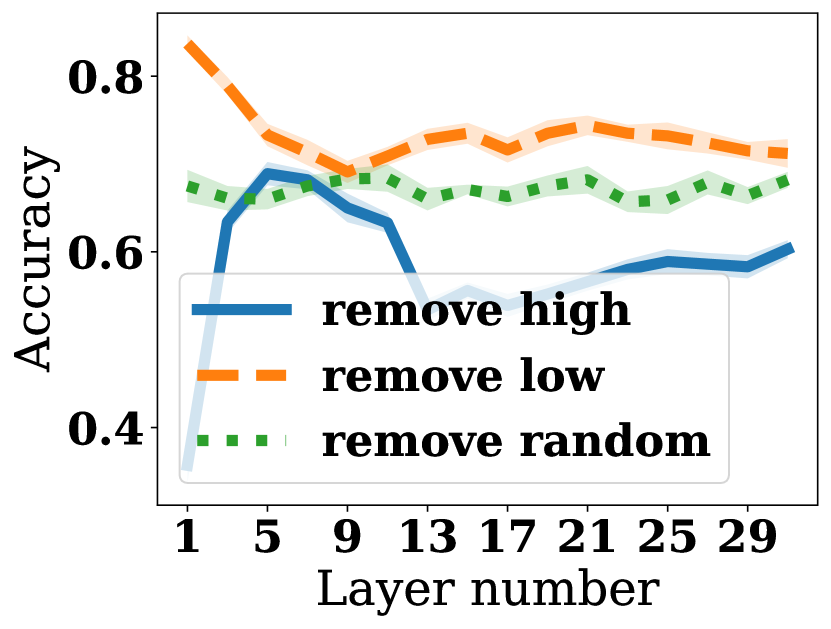
(a) Remove demonstration on Subj

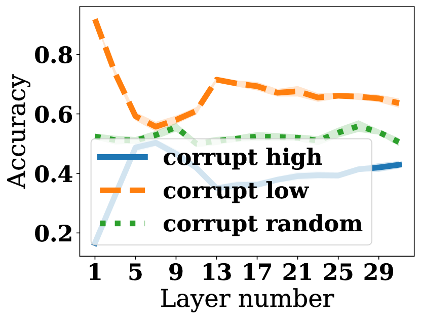
(b) Corrupt demonstration on Subj

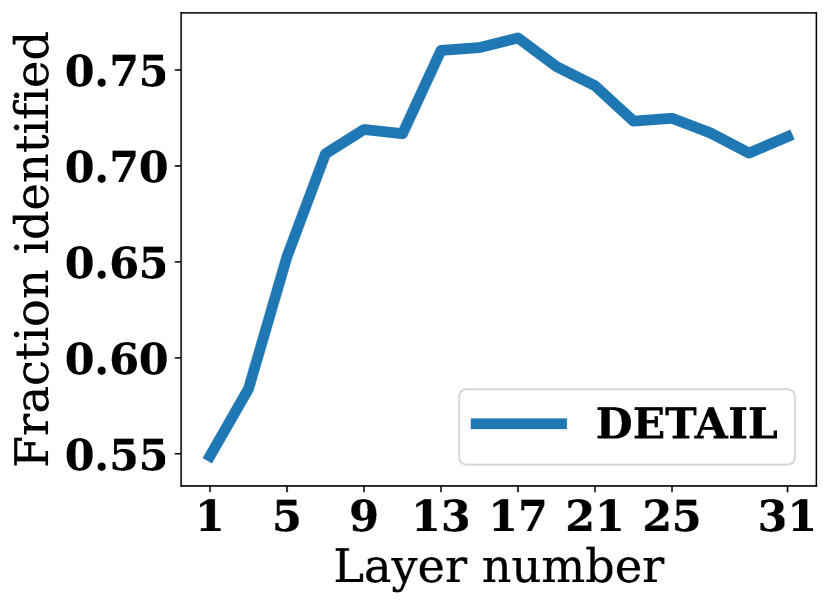
(c) Detecting noisy label on Subj

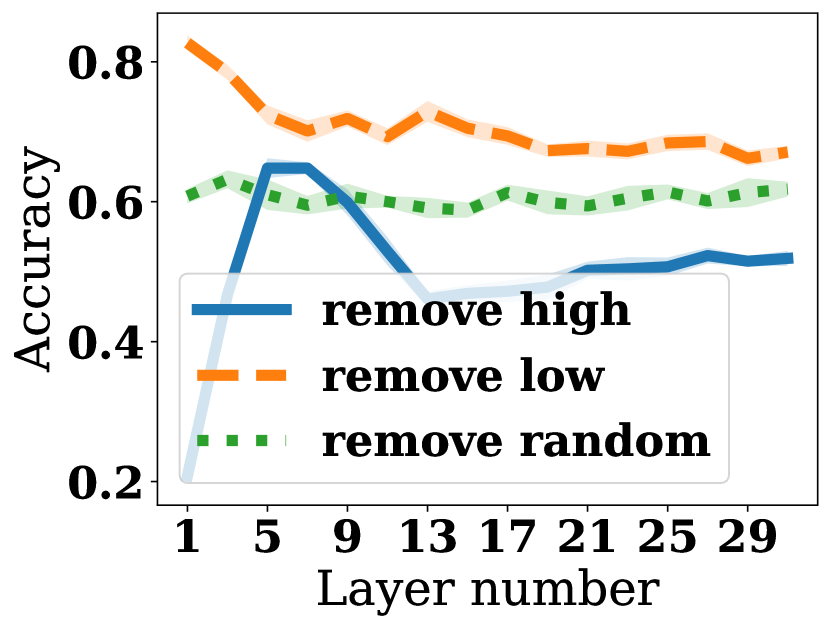
(d) Remove demonstration on SST-2

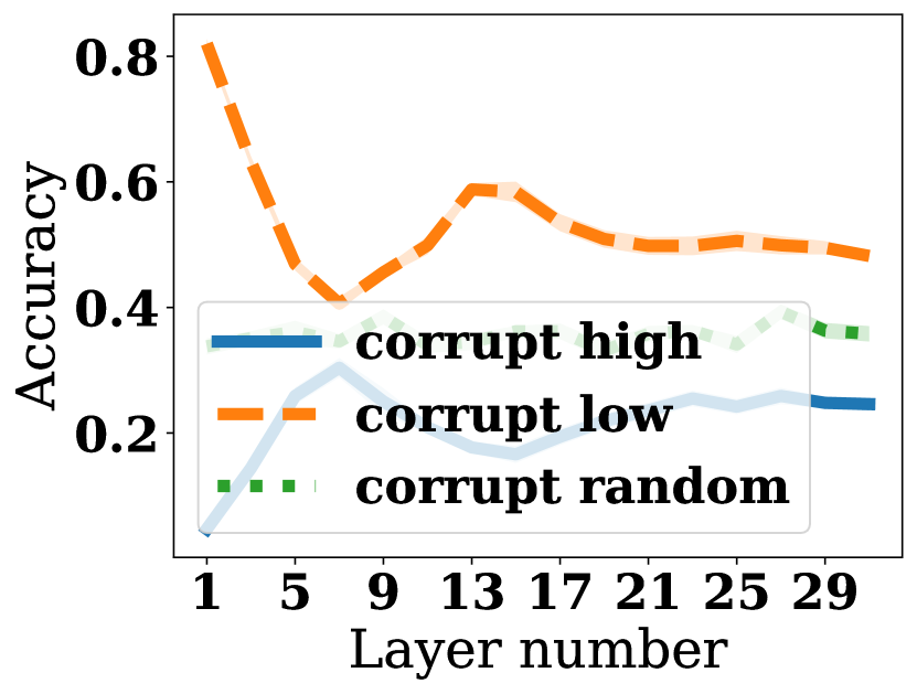
(e) Corrupt demonstration on SST-2

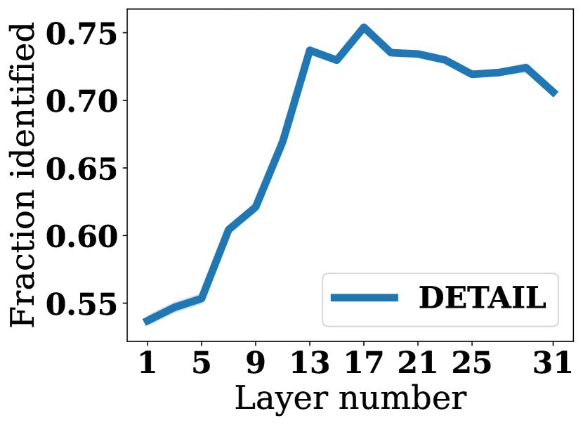
(f) Detecting noisy label on SST-2

Figure 13: Results of different task performance vs. the layer number in a Vicuna-7b model which consists of $31$ layers. Experiments are repeated with $10$ trials. $\lambda=1.0$ for (a,b,d,e) and $\lambda=10^{-9}$ for (c,f). Lines and shades represent the mean and standard error respectively.

D.7 Ablation of Target Position for Computing DETAIL.

As a rule of thumb, for each demonstration, we generally want to take the embedding of its last few tokens because of the causal nature of inference and because information generally flows toward the end of the sequence [49]. We compare two possible choices of target position: the column position (immediately before the label) and the label position. We experiment on the demonstration removal task with these two choices of embeddings. The results are shown in Fig. 14. Using embeddings of both positions achieves decent task performance as reflected by the clear distinction in accuracy between removing demonstrations with high/low DETAIL scores, demonstrating that our method is robust against the choice of token embeddings. In our experiments, we adopt the column position to isolate information about the label from the embedding.

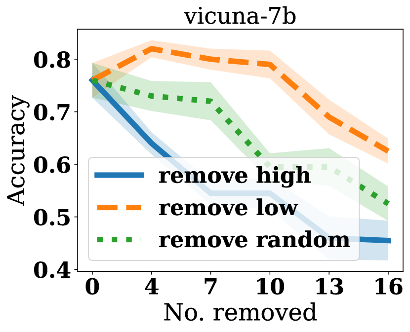
(a) Subj using label position

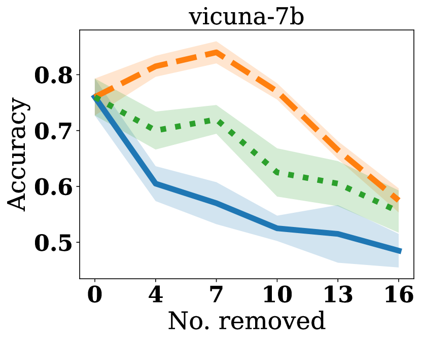
(b) Subj using column position

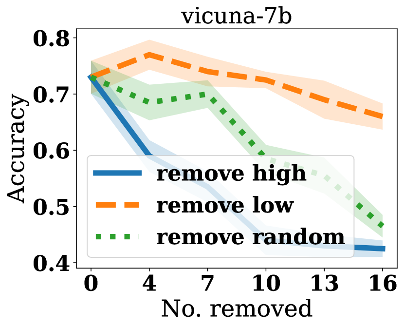
(c) SST-2 using label position

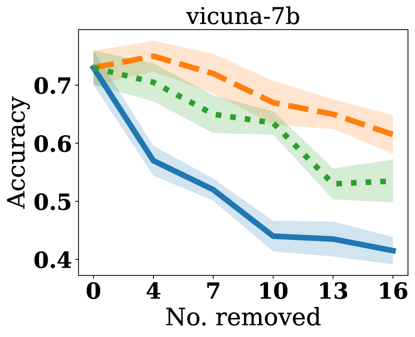
(d) SST-2 using column position

Figure 14: Results of model prediction accuracy vs. number of demonstrations removed using different positions for taking embeddings. $\lambda=1.0$. Lines and shades represent the mean and standard error respectively.

D.8 Experiment on State-Space Model Architecture

We consider experiments on a popular state-space model (SSM) architecture, a Mamba-2.8b model [23], which consists of $64$ layers with $d=2560$. The tasks are described in the main text in detail. While we find that DETAIL can still successfully attribute Mamba on certain tasks and datasets, the performance is inconsistent. One hypothesis is that the largest currently available Mamba model (2.8B) is still significantly smaller than the 7B LLMs we conduct experiments on in the main text. A smaller model size reduces the inductive power of the model to formulate the “internal optimizer”, leading to less interpretive DETAIL scores. We would also like to note that DETAIL is not designed to work on SSMs.

Demonstration removal.

The demonstration removal experiment follows the same setup as Sec. 5.2 but uses a Mamba-2.8b model instead, which is the largest model officially open-sourced. The results are shown in Fig. 15. Interestingly, removing demonstrations according to DETAIL scores still can influence predictive performance in the desirable manner where removing demonstrations with high $\mathcal{I}_{\text{test}}$ leads to lower accuracy and vice versa.

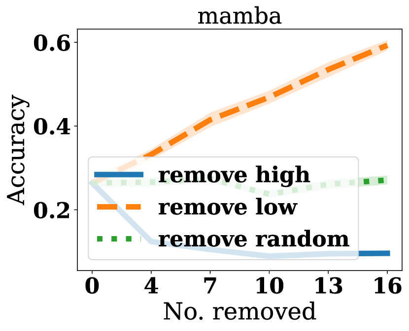
(a) AG News removal

(b) SST-2 removal

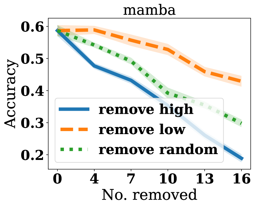
(c) Rotten Tomatoes removal

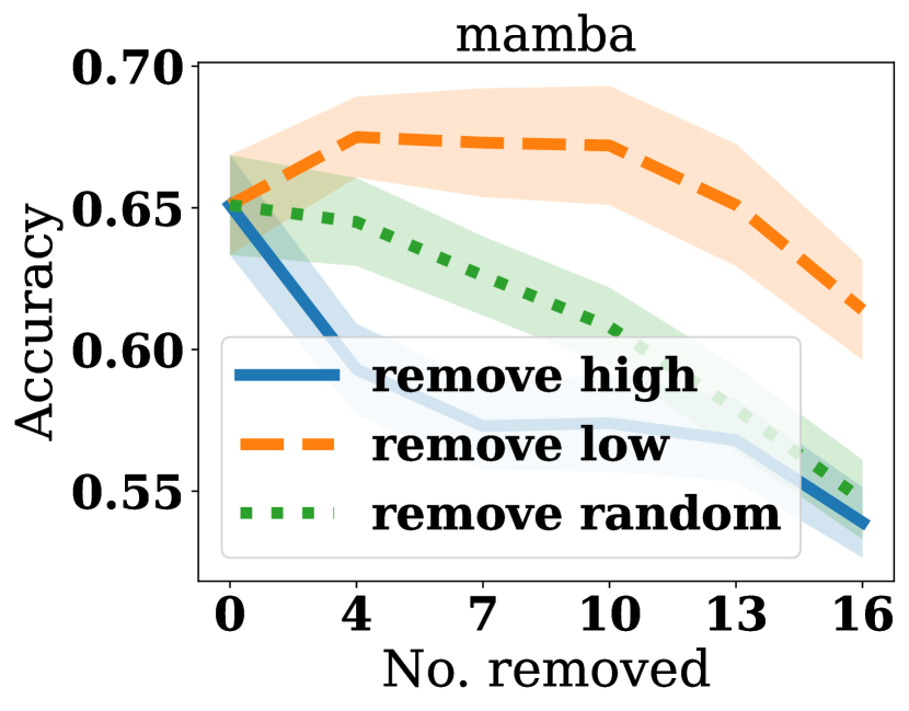
(d) Subj removal

Figure 15: Results of model prediction accuracy vs. number of demonstrations removed on Mamba. $\lambda=1.0$. Lines and shades represent the mean and standard error respectively.

Noisy demonstration detection.

We further consider the noisy demonstration detection task as described in Sec. 5.2 on Mamba. Unfortunately, the performance is not consistent across datasets, as shown in Fig. 16: detecting demonstrations with high $\mathcal{I}_{\text{self}}$ performs close to random selection on SST-2 and Rotten Tomatoes datasets, although the inference speedup is still significant. We leave the analysis of these failure cases to future work.

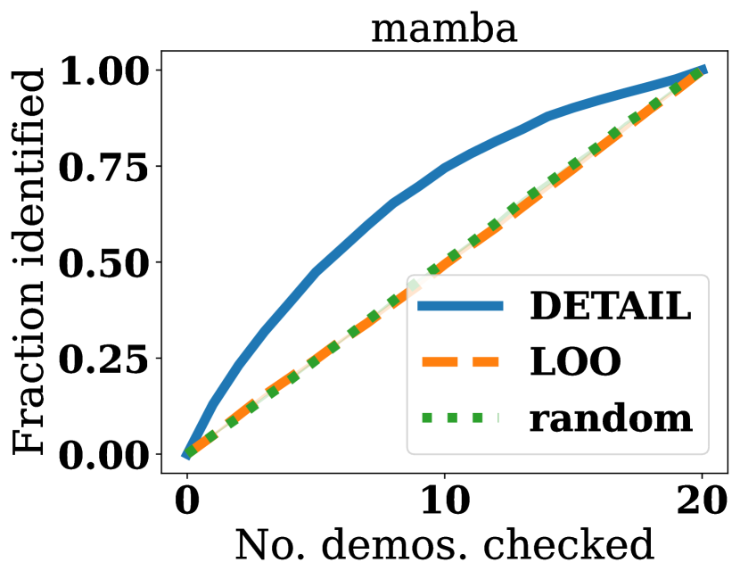
(a) Detecting noisy label on AG News

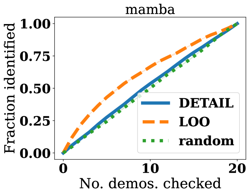
(b) Detecting noisy label on SST-2

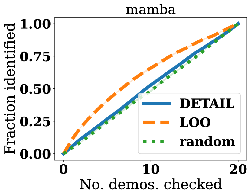
(c) Detecting noisy label on Rotten Tomatoes

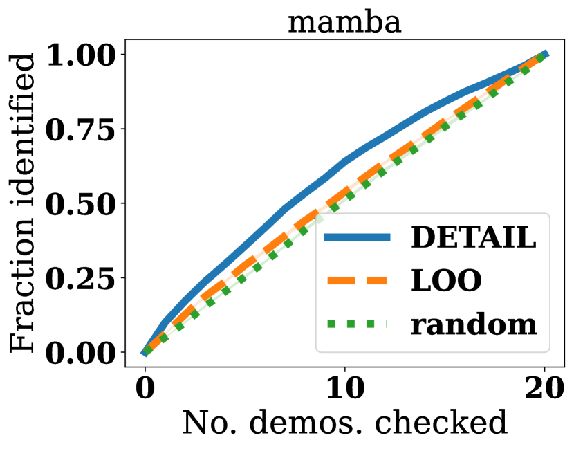
(d) Detecting noisy label on Subj

(e) Wall time comparison

Figure 16: (a-d) Fraction of all noisy labels identified vs. the number of demonstrations ranked by our method (with projection down to $1000$ dimension) and LOO checked respectively. (e) Wall time comparison across all datasets. $\lambda=10^{-9}$. All experiments are repeated with $10$ independent trials. Lines and shades represent the mean and standard error respectively.

Demonstration curation.

As DETAIL performs well using Mamba on the demonstration removal task, it is reasonable to hope that it works well on the demonstration curation task as well. As it turns out, DETAIL performs well on binary classification tasks as shown in Fig. 17 but performs poorly on AG News which is $4$-way classification. We hypothesize that this is due to Mamba’s worse inductive power to formulate an internal algorithm successfully.

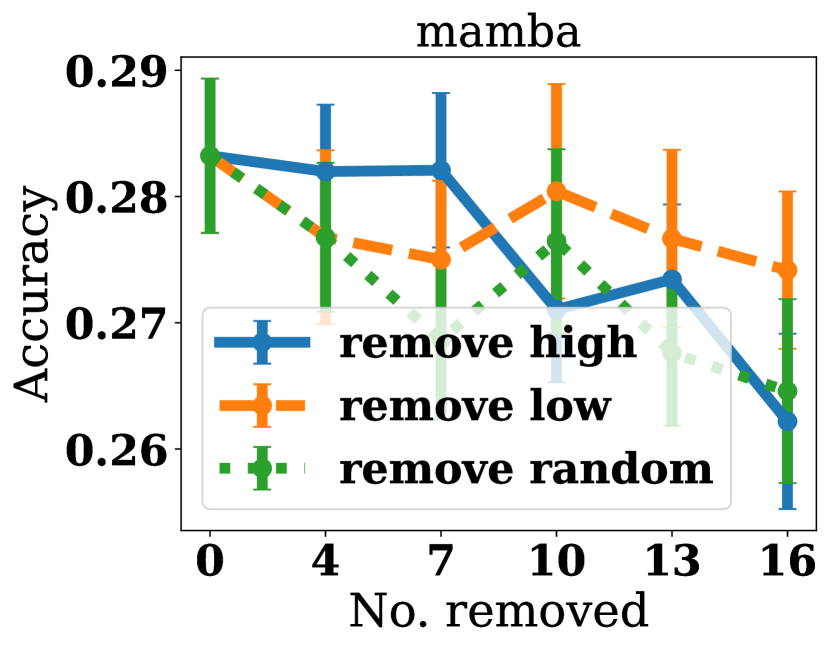
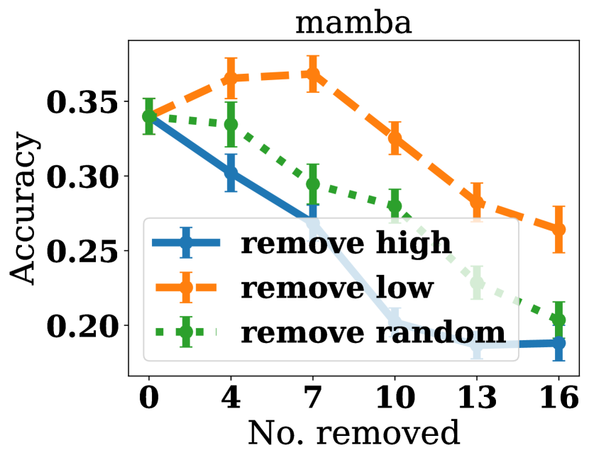
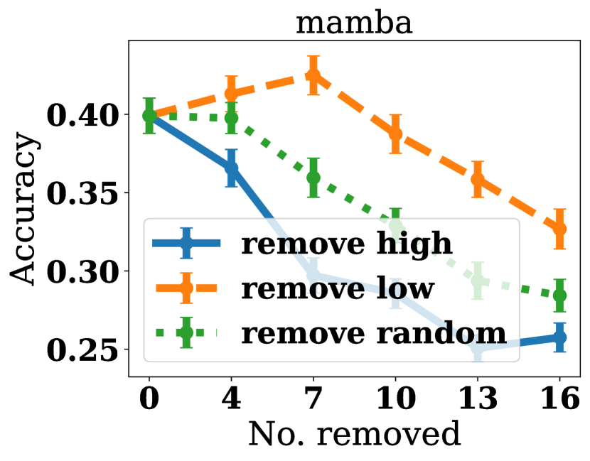
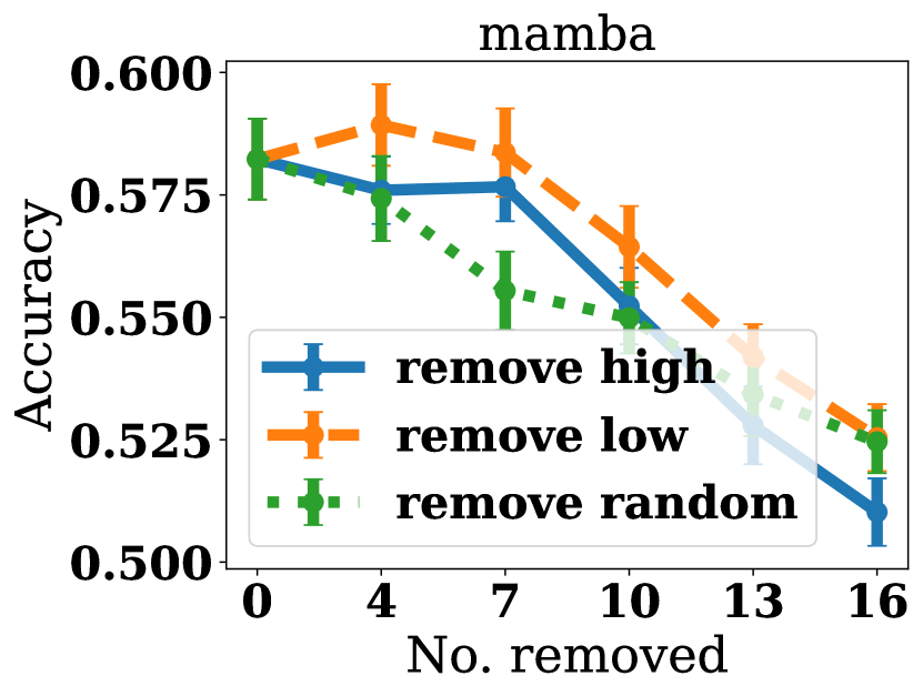
Figure 17: (Left to right) test accuracy vs. number of demonstrations removed using $\mathcal{I}_{\text{test}}$ on AG news, SST-2, Rotten Tomatoes, and Subj datasets using Mamba-2.8b. All experiments are repeated with $80$ independent trials. Lines and bars represent the mean and standard error respectively.

References

- Agarwal et al. [2017] Naman Agarwal, Brian Bullins, and Elad Hazan. Second-order stochastic optimization for machine learning in linear time. Journal of Machine Learning Research, 2017.
- Ahn et al. [2023] Kwangjun Ahn, Xiang Cheng, Hadi Daneshmand, and Suvrit Sra. Transformers learn to implement preconditioned gradient descent for in-context learning. In Advances in Neural Information Processing Systems, 2023.
- Akyürek et al. [2023] Ekin Akyürek, Dale Schuurmans, Jacob Andreas, Tengyu Ma, and Denny Zhou. What learning algorithm is in-context learning? investigations with linear models, 2023.
- Almazrouei et al. [2023] Ebtesam Almazrouei, Hamza Alobeidli, Abdulaziz Alshamsi, Alessandro Cappelli, Ruxandra Cojocaru, Mérouane Debbah, Étienne Goffinet, Daniel Hesslow, Julien Launay, Quentin Malartic, Daniele Mazzotta, Badreddine Noune, Baptiste Pannier, and Guilherme Penedo. The falcon series of open language models, 2023.
- Ansel et al. [2024] Jason Ansel, Edward Yang, Horace He, Natalia Gimelshein, Animesh Jain, Michael Voznesensky, Bin Bao, Peter Bell, David Berard, Evgeni Burovski, Geeta Chauhan, Anjali Chourdia, Will Constable, Alban Desmaison, Zachary DeVito, Elias Ellison, Will Feng, Jiong Gong, Michael Gschwind, Brian Hirsh, Sherlock Huang, Kshiteej Kalambarkar, Laurent Kirsch, Michael Lazos, Mario Lezcano, Yanbo Liang, Jason Liang, Yinghai Lu, CK Luk, Bert Maher, Yunjie Pan, Christian Puhrsch, Matthias Reso, Mark Saroufim, Marcos Yukio Siraichi, Helen Suk, Michael Suo, Phil Tillet, Eikan Wang, Xiaodong Wang, William Wen, Shunting Zhang, Xu Zhao, Keren Zhou, Richard Zou, Ajit Mathews, Gregory Chanan, Peng Wu, and Soumith Chintala. Pytorch 2: Faster machine learning through dynamic Python bytecode transformation and graph compilation. In ACM International Conference on Architectural Support for Programming Languages and Operating Systems, 2024.
- Bahdanau et al. [2016] Dzmitry Bahdanau, Kyunghyun Cho, and Yoshua Bengio. Neural machine translation by jointly learning to align and translate. In Proceedings of the International Conference on Learning Representations, 2016.
- Barshan et al. [2020] Elnaz Barshan, Marc-Etienne Brunet, and Gintare Karolina Dziugaite. Relatif: Identifying explanatory training samples via relative influence. In Proceedings of the International Conference on Artificial Intelligence and Statistics, 2020.
- Basu et al. [2021] Samyadeep Basu, Philip Pope, and Soheil Feizi. Influence functions in deep learning are fragile. In Proceedings of the International Conference on Learning Representations, 2021.
- Bohnet et al. [2022] Bernd Bohnet, Vinh Q. Tran, Pat Verga, Roee Aharoni, Daniel Andor, Livio Baldini Soares, Massimiliano Ciaramita, Jacob Eisenstein, Kuzman Ganchev, Jonathan Herzig, Kai Hui, Tom Kwiatkowski, Ji Ma, Jianmo Ni, Lierni Sestorain Saralegui, Tal Schuster, William W. Cohen, Michael Collins, Dipanjan Das, Donald Metzler, Slav Petrov, and Kellie Webster. Attributed question answering: Evaluation and modeling for attributed large language models, 2022. URL https://arxiv.org/abs/2212.08037.
- Bommasani et al. [2022] Rishi Bommasani, Drew A. Hudson, Ehsan Adeli, Russ Altman, Simran Arora, Sydney von Arx, Michael S. Bernstein, Jeannette Bohg, Antoine Bosselut, Emma Brunskill, Erik Brynjolfsson, Shyamal Buch, Dallas Card, Rodrigo Castellon, Niladri Chatterji, Annie Chen, Kathleen Creel, Jared Quincy Davis, Dora Demszky, Chris Donahue, Moussa Doumbouya, Esin Durmus, Stefano Ermon, John Etchemendy, Kawin Ethayarajh, Li Fei-Fei, Chelsea Finn, Trevor Gale, Lauren Gillespie, Karan Goel, Noah Goodman, Shelby Grossman, Neel Guha, Tatsunori Hashimoto, Peter Henderson, John Hewitt, Daniel E. Ho, Jenny Hong, Kyle Hsu, Jing Huang, Thomas Icard, Saahil Jain, Dan Jurafsky, Pratyusha Kalluri, Siddharth Karamcheti, Geoff Keeling, Fereshte Khani, Omar Khattab, Pang Wei Koh, Mark Krass, Ranjay Krishna, Rohith Kuditipudi, Ananya Kumar, Faisal Ladhak, Mina Lee, Tony Lee, Jure Leskovec, Isabelle Levent, Xiang Lisa Li, Xuechen Li, Tengyu Ma, Ali Malik, Christopher D. Manning, Suvir Mirchandani, Eric Mitchell, Zanele Munyikwa, Suraj Nair, Avanika Narayan, Deepak Narayanan, Ben Newman, Allen Nie, Juan Carlos Niebles, Hamed Nilforoshan, Julian Nyarko, Giray Ogut, Laurel Orr, Isabel Papadimitriou, Joon Sung Park, Chris Piech, Eva Portelance, Christopher Potts, Aditi Raghunathan, Rob Reich, Hongyu Ren, Frieda Rong, Yusuf Roohani, Camilo Ruiz, Jack Ryan, Christopher Ré, Dorsa Sadigh, Shiori Sagawa, Keshav Santhanam, Andy Shih, Krishnan Srinivasan, Alex Tamkin, Rohan Taori, Armin W. Thomas, Florian Tramèr, Rose E. Wang, William Wang, Bohan Wu, Jiajun Wu, Yuhuai Wu, Sang Michael Xie, Michihiro Yasunaga, Jiaxuan You, Matei Zaharia, Michael Zhang, Tianyi Zhang, Xikun Zhang, Yuhui Zhang, Lucia Zheng, Kaitlyn Zhou, and Percy Liang. On the opportunities and risks of foundation models, 2022.
- Bradbury et al. [2018] James Bradbury, Roy Frostig, Peter Hawkins, Matthew James Johnson, Chris Leary, Dougal Maclaurin, George Necula, Adam Paszke, Jake VanderPlas, Skye Wanderman-Milne, and Qiao Zhang. JAX: composable transformations of Python+NumPy programs, 2018. URL http://github.com/google/jax.
- Brown et al. [2020] Tom Brown, Benjamin Mann, Nick Ryder, Melanie Subbiah, Jared D Kaplan, Prafulla Dhariwal, Arvind Neelakantan, Pranav Shyam, Girish Sastry, Amanda Askell, Sandhini Agarwal, Ariel Herbert-Voss, Gretchen Krueger, Tom Henighan, Rewon Child, Aditya Ramesh, Daniel Ziegler, Jeffrey Wu, Clemens Winter, Chris Hesse, Mark Chen, Eric Sigler, Mateusz Litwin, Scott Gray, Benjamin Chess, Jack Clark, Christopher Berner, Sam McCandlish, Alec Radford, Ilya Sutskever, and Dario Amodei. Language models are few-shot learners. In Advances in Neural Information Processing Systems, 2020.
- Chang & Jia [2023] Ting-Yun Chang and Robin Jia. Data curation alone can stabilize in-context learning. In Proceedings of the Annual Meeting of the Association for Computational Linguistics, 2023.
- Chen et al. [2024] Siyu Chen, Heejune Sheen, Tianhao Wang, and Zhuoran Yang. Training dynamics of multi-head softmax attention for in-context learning: Emergence, convergence, and optimality, 2024.
- Chowdhery et al. [2022] Aakanksha Chowdhery, Sharan Narang, Jacob Devlin, Maarten Bosma, Gaurav Mishra, Adam Roberts, Paul Barham, Hyung Won Chung, Charles Sutton, Sebastian Gehrmann, Parker Schuh, Kensen Shi, Sasha Tsvyashchenko, Joshua Maynez, Abhishek Rao, Parker Barnes, Yi Tay, Noam Shazeer, Vinodkumar Prabhakaran, Emily Reif, Nan Du, Ben Hutchinson, Reiner Pope, James Bradbury, Jacob Austin, Michael Isard, Guy Gur-Ari, Pengcheng Yin, Toju Duke, Anselm Levskaya, Sanjay Ghemawat, Sunipa Dev, Henryk Michalewski, Xavier Garcia, Vedant Misra, Kevin Robinson, Liam Fedus, Denny Zhou, Daphne Ippolito, David Luan, Hyeontaek Lim, Barret Zoph, Alexander Spiridonov, Ryan Sepassi, David Dohan, Shivani Agrawal, Mark Omernick, Andrew M. Dai, Thanumalayan Sankaranarayana Pillai, Marie Pellat, Aitor Lewkowycz, Erica Moreira, Rewon Child, Oleksandr Polozov, Katherine Lee, Zongwei Zhou, Xuezhi Wang, Brennan Saeta, Mark Diaz, Orhan Firat, Michele Catasta, Jason Wei, Kathy Meier-Hellstern, Douglas Eck, Jeff Dean, Slav Petrov, and Noah Fiedel. Palm: Scaling language modeling with pathways, 2022.
- Conneau & Kiela [2018] Alexis Conneau and Douwe Kiela. Senteval: An evaluation toolkit for universal sentence representations. In Proceedings of the International Conference on Language Resources and Evaluation, 2018.
- Cook [1977] R. Dennis. Cook. Detection of influential observation in linear regression. Technometrics, 1977.
- Dasgupta & Gupta [2003] Sanjoy Dasgupta and Anupam Gupta. An elementary proof of a theorem of Johnson and Lindenstrauss. Random Structures & Algorithms, 2003.
- Deng [2012] Li Deng. The MNIST database of handwritten digit images for machine learning research. IEEE Signal Processing Magazine, 2012.
- Garg et al. [2023] Shivam Garg, Dimitris Tsipras, Percy Liang, and Gregory Valiant. What can transformers learn in-context? A case study of simple function classes, 2023.
- Ghorbani & Zou [2019] Amirata Ghorbani and James Zou. Data Shapley: Equitable valuation of data for machine learning. In Proceedings of the International Conference on Machine Learning, 2019.
- Grosse et al. [2023] Roger Grosse, Juhan Bae, Cem Anil, Nelson Elhage, Alex Tamkin, Amirhossein Tajdini, Benoit Steiner, Dustin Li, Esin Durmus, Ethan Perez, Evan Hubinger, Kamilė Lukošiūtė, Karina Nguyen, Nicholas Joseph, Sam McCandlish, Jared Kaplan, and Samuel R. Bowman. Studying large language model generalization with influence functions, 2023.
- Gu & Dao [2023] Albert Gu and Tri Dao. Mamba: Linear-time sequence modeling with selective state spaces, 2023.
- Hainmueller & Hazlett [2014] Jens Hainmueller and Chad Hazlett. Kernel regularized least squares: Reducing misspecification bias with a flexible and interpretable machine learning approach. Political analysis, 2014.
- Hu et al. [2022] Edward J Hu, Yelong Shen, Phillip Wallis, Zeyuan Allen-Zhu, Yuanzhi Li, Shean Wang, Lu Wang, and Weizhu Chen. LoRA: Low-rank adaptation of large language models. In Proceedings of the International Conference on Learning Representations, 2022.
- Johnson & Lindenstrauss [1984] William Johnson and Joram Lindenstrauss. Extensions of Lipschitz maps into a Hilbert space. Contemporary Mathematics, 1984.
- Koh & Liang [2017] Pang Wei Koh and Percy Liang. Understanding black-box predictions via influence functions. In Proceedings of the International Conference on Machine Learning, 2017.
- Kwon et al. [2024] Yongchan Kwon, Eric Wu, Kevin Wu, and James Zou. DataInf: Efficiently estimating data influence in LoRA-tuned LLMs and diffusion models. In Proceedings of the International Conference on Learning Representations, 2024.
- Lhoest et al. [2021] Quentin Lhoest, Albert Villanova del Moral, Yacine Jernite, Abhishek Thakur, Patrick von Platen, Suraj Patil, Julien Chaumond, Mariama Drame, Julien Plu, Lewis Tunstall, Joe Davison, Mario Šaško, Gunjan Chhablani, Bhavitvya Malik, Simon Brandeis, Teven Le Scao, Victor Sanh, Canwen Xu, Nicolas Patry, Angelina McMillan-Major, Philipp Schmid, Sylvain Gugger, Clément Delangue, Théo Matussière, Lysandre Debut, Stas Bekman, Pierric Cistac, Thibault Goehringer, Victor Mustar, François Lagunas, Alexander Rush, and Thomas Wolf. Datasets: A community library for natural language processing. In Proceedings of the Conference on Empirical Methods in Natural Language Processing, 2021.
- Li et al. [2023] Yingcong Li, M. Emrullah Ildiz, Dimitris Papailiopoulos, and Samet Oymak. Transformers as algorithms: generalization and stability in in-context learning. In Proceedings of the International Conference on Machine Learning, 2023.
- Liu et al. [2023a] Hanxi Liu, Xiaokai Mao, Haocheng Xia, Jian Lou, and Jinfei Liu. Prompt valuation based on Shapley values, 2023a.
- Liu et al. [2023b] Nelson F. Liu, Kevin Lin, John Hewitt, Ashwin Paranjape, Michele Bevilacqua, Fabio Petroni, and Percy Liang. Lost in the middle: How language models use long contexts. Transactions of the Association for Computational Linguistics, 2023b.
- Liu et al. [2023c] Nelson F. Liu, Tianyi Zhang, and Percy Liang. Evaluating verifiability in generative search engines, 2023c.
- Lu et al. [2022] Yao Lu, Max Bartolo, Alastair Moore, Sebastian Riedel, and Pontus Stenetorp. Fantastically ordered prompts and where to find them: Overcoming few-shot prompt order sensitivity. In Proceedings of the Annual Meeting of the Association for Computational Linguistics, 2022.
- Machiraju et al. [2024] Gautam Machiraju, Alexander Derry, Arjun Desai, Neel Guha, Amir-Hossein Karimi, James Zou, Russ Altman, Christopher Ré, and Parag Mallick. Prospector heads: Generalized feature attribution for large models & data, 2024.
- Mitchell et al. [2022] Rory Mitchell, Joshua Cooper, Eibe Frank, and Geoffrey Holmes. Sampling permutations for Shapley value estimation. Journal of Machine Learning Research, 2022.
- Murphy [2012] Kevin P. Murphy. Machine Learning: A Probabilistic Perspective. The MIT Press, 2012.
- Nguyen & Wong [2023] Tai Nguyen and Eric Wong. In-context example selection with influences, 2023.
- Olsson et al. [2022] Catherine Olsson, Nelson Elhage, Neel Nanda, Nicholas Joseph, Nova DasSarma, Tom Henighan, Ben Mann, Amanda Askell, Yuntao Bai, Anna Chen, Tom Conerly, Dawn Drain, Deep Ganguli, Zac Hatfield-Dodds, Danny Hernandez, Scott Johnston, Andy Jones, Jackson Kernion, Liane Lovitt, Kamal Ndousse, Dario Amodei, Tom Brown, Jack Clark, Jared Kaplan, Sam McCandlish, and Chris Olah. In-context learning and induction heads, 2022.
- Pang & Lee [2005] Bo Pang and Lillian Lee. Seeing stars: Exploiting class relationships for sentiment categorization with respect to rating scales. In Proceedings of the Annual Meeting of the Association for Computational Linguistics, 2005.
- Ribeiro et al. [2016] Marco Tulio Ribeiro, Sameer Singh, and Carlos Guestrin. "Why should I trust you?": Explaining the predictions of any classifier. In Proceedings of the ACM SIGKDD International Conference on Knowledge Discovery and Data Mining, 2016.
- S. et al. [2024] Vinay M. S., Minh-Hao Van, and Xintao Wu. In-context learning demonstration selection via influence analysis, 2024.
- Sarti et al. [2023] Gabriele Sarti, Nils Feldhus, Ludwig Sickert, Oskar van der Wal, Malvina Nissim, and Arianna Bisazza. Inseq: An interpretability toolkit for sequence generation models. In Proceedings of the Annual Meeting of the Association for Computational Linguistics, 2023.
- Socher et al. [2013] Richard Socher, Alex Perelygin, Jean Wu, Jason Chuang, Christopher D. Manning, Andrew Ng, and Christopher Potts. Recursive deep models for semantic compositionality over a sentiment treebank. In Proceedings of the Conference on Empirical Methods in Natural Language Processing, 2013.
- Sundararajan et al. [2017] Mukund Sundararajan, Ankur Taly, and Qiqi Yan. Axiomatic attribution for deep networks. In Proceedings of the International Conference on Machine Learning, 2017.
- Touvron et al. [2023] Hugo Touvron, Louis Martin, Kevin Stone, Peter Albert, Amjad Almahairi, Yasmine Babaei, Nikolay Bashlykov, Soumya Batra, Prajjwal Bhargava, Shruti Bhosale, Dan Bikel, Lukas Blecher, Cristian Canton Ferrer, Moya Chen, Guillem Cucurull, David Esiobu, Jude Fernandes, Jeremy Fu, Wenyin Fu, Brian Fuller, Cynthia Gao, Vedanuj Goswami, Naman Goyal, Anthony Hartshorn, Saghar Hosseini, Rui Hou, Hakan Inan, Marcin Kardas, Viktor Kerkez, Madian Khabsa, Isabel Kloumann, Artem Korenev, Punit Singh Koura, Marie-Anne Lachaux, Thibaut Lavril, Jenya Lee, Diana Liskovich, Yinghai Lu, Yuning Mao, Xavier Martinet, Todor Mihaylov, Pushkar Mishra, Igor Molybog, Yixin Nie, Andrew Poulton, Jeremy Reizenstein, Rashi Rungta, Kalyan Saladi, Alan Schelten, Ruan Silva, Eric Michael Smith, Ranjan Subramanian, Xiaoqing Ellen Tan, Binh Tang, Ross Taylor, Adina Williams, Jian Xiang Kuan, Puxin Xu, Zheng Yan, Iliyan Zarov, Yuchen Zhang, Angela Fan, Melanie Kambadur, Sharan Narang, Aurelien Rodriguez, Robert Stojnic, Sergey Edunov, and Thomas Scialom. Llama 2: Open foundation and fine-tuned chat models, 2023.
- Von Oswald et al. [2023] Johannes Von Oswald, Eyvind Niklasson, Ettore Randazzo, João Sacramento, Alexander Mordvintsev, Andrey Zhmoginov, and Max Vladymyrov. Transformers learn in-context by gradient descent. In Proceedings of the International Conference on Machine Learning, 2023.
- von Oswald et al. [2023] Johannes von Oswald, Eyvind Niklasson, Maximilian Schlegel, Seijin Kobayashi, Nicolas Zucchet, Nino Scherrer, Nolan Miller, Mark Sandler, Blaise Agüera y Arcas, Max Vladymyrov, Razvan Pascanu, and João Sacramento. Uncovering mesa-optimization algorithms in transformers, 2023.
- Wang et al. [2023] Lean Wang, Lei Li, Damai Dai, Deli Chen, Hao Zhou, Fandong Meng, Jie Zhou, and Xu Sun. Label words are anchors: An information flow perspective for understanding in-context learning. In Proceedings of the Conference on Empirical Methods in Natural Language Processing, 2023.
- Wei et al. [2023] Jason Wei, Xuezhi Wang, Dale Schuurmans, Maarten Bosma, Brian Ichter, Fei Xia, Ed Chi, Quoc Le, and Denny Zhou. Chain-of-thought prompting elicits reasoning in large language models. In Advances in Neural Information Processing Systems, 2023.
- Wolf et al. [2020] Thomas Wolf, Lysandre Debut, Victor Sanh, Julien Chaumond, Clement Delangue, Anthony Moi, Pierric Cistac, Tim Rault, Rémi Louf, Morgan Funtowicz, Joe Davison, Sam Shleifer, Patrick von Platen, Clara Ma, Yacine Jernite, Julien Plu, Canwen Xu, Teven Le Scao, Sylvain Gugger, Mariama Drame, Quentin Lhoest, and Alexander M. Rush. Transformers: State-of-the-art natural language processing. In Proceedings of the Conference on Empirical Methods in Natural Language Processing, 2020.
- Xia et al. [2024] Mengzhou Xia, Sadhika Malladi, Suchin Gururangan, Sanjeev Arora, and Danqi Chen. Less: Selecting influential data for targeted instruction tuning, 2024.
- Xie et al. [2022] Sang Michael Xie, Aditi Raghunathan, Percy Liang, and Tengyu Ma. An explanation of in-context learning as implicit Bayesian inference. In Proceedings of the International Conference on Learning Representations, 2022.
- Yao et al. [2023] Shunyu Yao, Dian Yu, Jeffrey Zhao, Izhak Shafran, Thomas L. Griffiths, Yuan Cao, and Karthik Narasimhan. Tree of Thoughts: Deliberate problem solving with large language models. In Advances in Neural Information Processing Systems, 2023.
- Yue et al. [2023] Xiang Yue, Boshi Wang, Kai Zhang, Ziru Chen, Yu Su, and Huan Sun. Automatic evaluation of attribution by large language models. arXiv preprint arXiv:2305.06311, 2023.
- Zhang et al. [2024a] Ruiqi Zhang, Spencer Frei, and Peter L. Bartlett. Trained transformers learn linear models in-context. Journal of Machine Learning Research, 2024a.
- Zhang et al. [2024b] Shaokun Zhang, Xiaobo Xia, Zhaoqing Wang, Ling-Hao Chen, Jiale Liu, Qingyun Wu, and Tongliang Liu. Ideal: Influence-driven selective annotations empower in-context learners in large language models. In Proceedings of the International Conference on Learning Representations, 2024b.
- Zhang et al. [2015] Xiang Zhang, Junbo Jake Zhao, and Yann LeCun. Character-level convolutional networks for text classification. In Advances in Neural Information Processing Systems, 2015.
- Zheng et al. [2023] Lianmin Zheng, Wei-Lin Chiang, Ying Sheng, Siyuan Zhuang, Zhanghao Wu, Yonghao Zhuang, Zi Lin, Zhuohan Li, Dacheng Li, Eric. P Xing, Hao Zhang, Joseph E. Gonzalez, and Ion Stoica. Judging LLM-as-a-judge with MT-bench and chatbot arena. In Advances in Neural Information Processing Systems, 2023.