LookUp3D: Data-Driven 3D Scanning

Abstract.

We introduce a novel calibration and reconstruction procedure for structured light scanning that foregoes explicit point triangulation in favor of a data-driven lookup procedure. The key idea is to sweep a calibration checkerboard over the entire scanning volume with a linear stage and acquire a dense stack of images to build a per-pixel lookup table from colors to depths. Imperfections in the setup, lens distortion, and sensor defects are baked into the calibration data, leading to a more reliable and accurate reconstruction. Existing structured light scanners can be reused without modifications while enjoying the superior precision and resilience that our calibration and reconstruction algorithms offer. Our algorithm shines when paired with a custom-designed analog projector, which enables 1 megapixel slow-motion 3D scanning at up to 500 fps.

We describe our algorithm and hardware prototype for slow-motion 3D scanning and compare them with commercial and open-source structured light scanning methods.

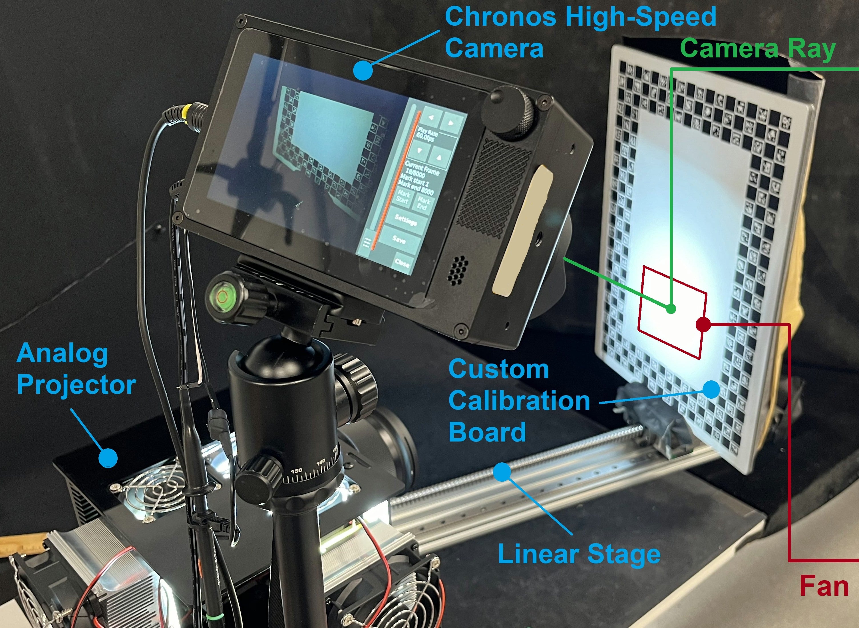
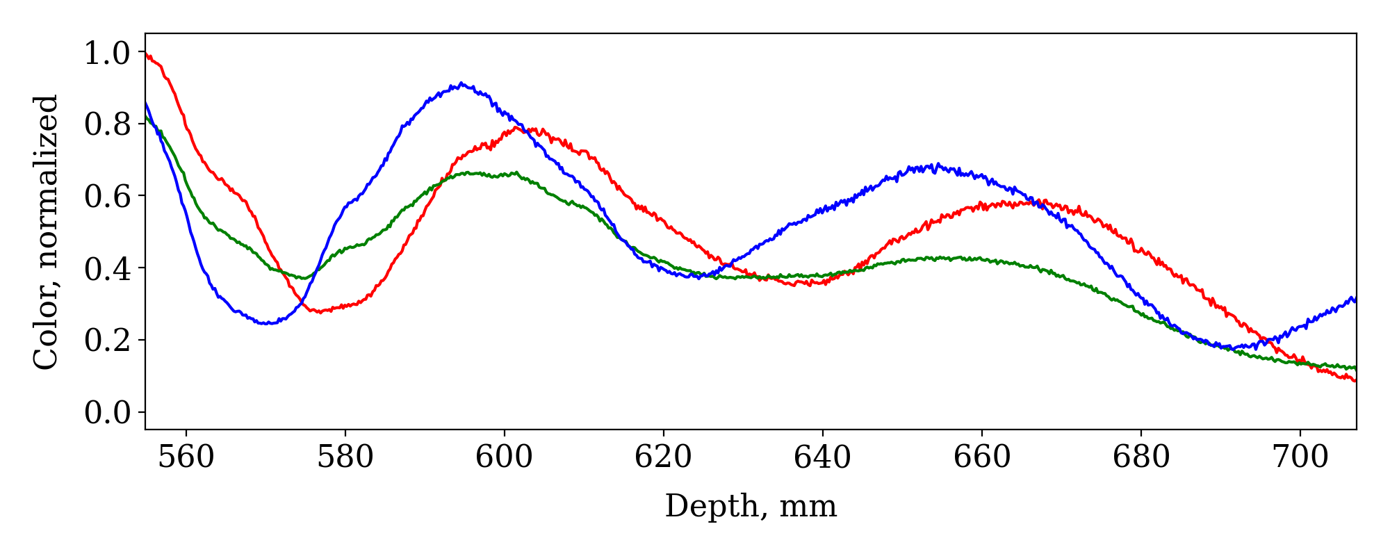
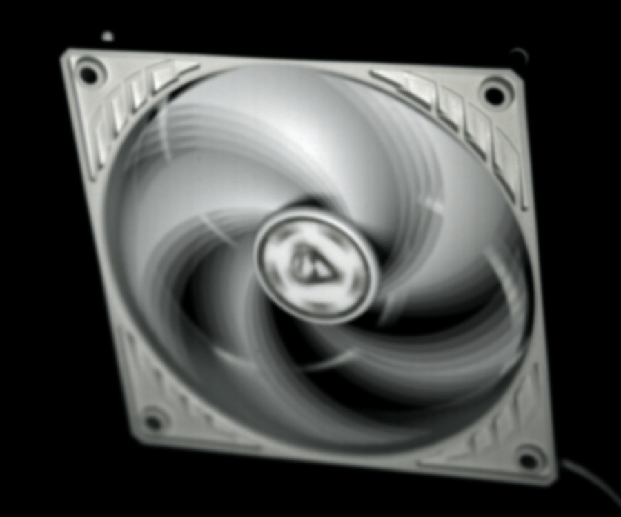
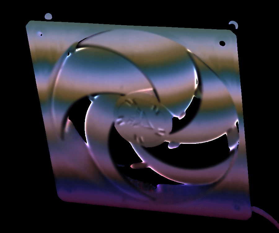
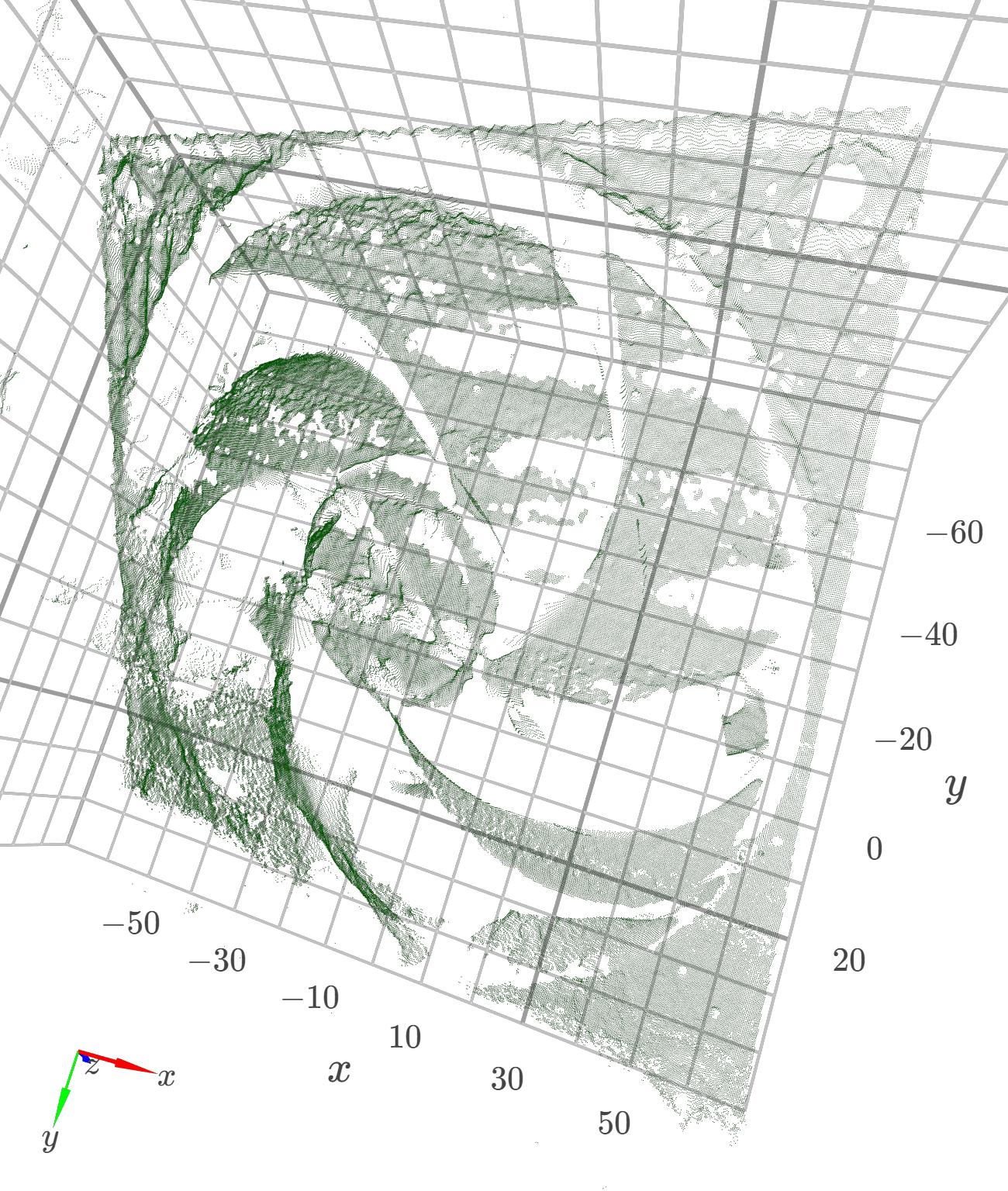
Figure 1. LookUp3D uses an analog projector to acquire slow-motion depth sequences. The reconstruction algorithm relies on calibration data acquired by covering the entire calibration volume with a moving calibration board. In this example, we are acquiring a fan spinning at 300 rpm.

1. Introduction

3D geometry acquisition is ubiquitous in our lives, with its use in face recognition, car navigation, manufacturing, and virtual reality. Various hardware solutions have been introduced to tackle this problem, using touch, time-of-flight, stereo imaging, structured light, x-rays, or magnetic resonance (Section 2).

Structured Light.

Structured light (using visible or non-visible frequencies) is popular due to its high resolution and possibility for acquisition of moving objects, with frame rates up to 90fps. Many of us use it daily to 3D scan our faces to unlock digital devices. A structured light scanner usually comprises a projector and a camera. An initial calibration is used to create a model of the scanner by estimating the intrinsic and extrinsic parameters of the camera and projector. The model is then used to triangulate points in the scene by projecting a unique code per pixel and decoding it on the image plane. The quality of the reconstruction depends on the accuracy of the model used to simulate the camera and projector, usually leading to the use of expensive electronics and high-quality lenses in the hardware setup (Koch et al., 2021) to achieve high resolution and accuracy. The calibration of the scanner leads to a small set of parameters describing the geometry of the scanner and lenses for the camera and projector (Lanman and Taubin, 2009a). When many patterns are used, this approach is limited to objects moving at low speed due to the necessity of projecting and acquiring multiple coded patterns for each depth reconstruction. For fast-moving objects, the different patterns are projected on a different, moving geometry and thus create large reconstruction errors.

Our Contribution.

We introduce LookUp3D (LU3D), a novel structured light scanning approach that eliminates the need for a digital twin model, relying entirely on the raw calibration data for 3D reconstruction. Our core observation is that it is not necessary to use the calibration procedure to fit a low-parametric scanner model, as the model’s accuracy will be an upper bound on the reconstruction accuracy. Instead, we extend the calibration procedure to acquire a dense per-pixel function mapping colors to depth: that is, during calibration, we acquire normalized colors for all possible depth values; with this data, the reconstruction is a search on a per-pixel color lookup table. While at first glance, this might seem unwieldy in terms of calibration complexity, time, and storage, we show that this is not the case: the calibration can be performed in 10 minutes with a motorized uni-axial linear stage with a large calibration board mounted on top; the storage of the calibration data is less than 10 Gb; and the reconstruction time of our CPU-only implementation is around 3 seconds per frame.

We evaluate our approach in two complementary settings: (1) to compare with existing structured light methods, we use our calibration and reconstruction procedure using existing structured light hardware and patterns, and (2) we propose a novel analog projector with a single pattern exploiting the additional flexibility that our method offers, enabling slow-motion 3D depth sensing.

Existing Hardware.

Interestingly, we can use the existing hardware without modifications, we only need to use our calibration device, leading to a slightly longer calibration time. The benefit of our approach is an increase in precision and similar accuracy. On the downside, our approach is less resilient to specularities, which are captured as surface bumps.

Slow-Motion Depth Scanning.

A key benefit of our approach is that we do not require a specific sequence of patterns — any pattern sequence can be used in our calibration and reconstruction procedure, even a sequence of random patterns. We study in Section 4 the effect of using different patterns and, after extensive analysis and experimentation, we show that a single pattern with three channels (RGB image) is sufficient for high-quality reconstruction. The use of a single pattern enables us to replace the digital projector with a custom analog projector composed of two LED lights, a beam splitter, a camera lens, and a 35mm film slide. The analog projector has significant advantages over the digital one of supporting a higher framerate and a lower cost and complexity. When the analog projector is paired with a high-speed camera, we obtain a high-speed acquisition system for 3D geometry at framerates up to 500 fps at a 1 megapixel resolution. Interestingly, the calibration and the reconstruction algorithm are identical to the setup above, making our approach very flexible and adaptable to specific 3D acquisition requirements.

Contributions.

Our major contributions are:

1. A novel approach for structured light 3D scanning. This includes novel calibration hardware and a simple yet novel and effective reconstruction algorithm.

2. An analysis of this approach using a standard structured light 3D scanner.

3. An analysis of patterns in the context of our reconstruction method. The analysis led to the design of the Spiral pattern as the preferred option for RGB single-exposure.

4. A hybrid scanner hardware comprising a digital camera and an analog projector that enables depth acquisition at 400 fps and a 1 megapixel resolution.

We believe our contribution will have a major impact on the multitude of applications requiring the acquisition of 3D data, as it opens the door to high-quality and high-framerate scanning with low-cost hardware.

2. Related Work

There is a large literature on the acquisition of 3D geometry (Lanman and Taubin, 2009b), using a variety of hardware solutions including touch probes (Ferreira et al., 2013; Dobosz and Woźniak, 2005), time-of-flight cameras (Horaud et al., 2016; Gao et al., 2015; Tang et al., 2010), structured light (Zhang, 2018; Salvi et al., 2004), and stereo reconstruction (Furukawa and Hernández, 2015). We focus our review on structured light scanning (SLS) methods as they are popular due to their quality and accuracy tradeoffs and they are the closest to our method.

Structured Light Scanning.

(Zhang, 2018) provides an overview of structured light scanning (SLS) methods. SLS is a non-contact active technique where we emit light and detect its reflection to probe the shape of the scene. This is often done by triangulating matching samples from calibrated projector and camera pairs. We refer to (Lanman and Taubin, 2009a)’s excellent tutorial for detailed coverage of the triangulation process and how to perform camera and projector calibration and to (Koch et al., 2021) for a detailed open-hardware and open-software implementation.

SLS approaches strive to triangulate a point by finding an intersection between a camera ray and a projector plane. The wide range of techniques proposed varies the number or types of patterns projected (Salvi et al., 2004), the number of cameras and projectors used, and the technique to extract the projector plane from the image data.

(Posdamer and Altschuler, 1982) pioneered the area by proposing to use a sequence of $m$ image patterns to encode $2^{m}$ stripes using a plain binary code (Hall-Holt and Rusinkiewicz, 2001), further improved by (Inokuchi et al., 1984) using Gray codes. (Carrihill and Hummel, 1985) proposes linear patterns. (Boyer and Kak, 1987; Caspi et al., 1998; Je et al., 2012) stack 3 patterns into a RGB image. A major breakthrough is the use of 3 phase-shifted overlapping color fringes (Wust and Capson, 1991; Gupta and Nayar, 2012).

In all these methods, the accuracy is inherently limited by the need to do triangulation, and they require an involved procedure to reconstruct the projector plane from the image. We propose a novel approach that uses the projected colors to directly encode a per-pixel depth, avoiding the need for triangulation. We perform a comparison against the more common patterns proposed by these approaches (binary and continuous) in Section 5.

Slow-Motion 3D Scanning.

(Zhang et al., 2010) proposes the use of a DLP projector (usually limited to 120fps) in binary mode, with special hardware that converts it into a phase-shifting pattern. In binary mode, the projector can dramatically increase its framerate (up to a few thousand fps), allowing it to acquire range scans at 667 fps. The paper is however only showing static reconstructions, and their approach has a negative impact on the intensity of the projector, which is crucial for high-speed acquisition. We propose an analog projector that allows us to acquire a range scan with only two patterns, one of them with three color channels (Section 6), which enables for the design of efficient high-speed projectors given adequate engineering resources.

Commercial Solutions.

SLS has been used successfully in commercial products. For instance, the first version of Microsoft Kinect (Anon, 2023a) was based on the structured light system originally developed by PrimeSense (Anon, 2023c). We compare our work with three commercial scanners: the Microsoft Kinect, the Intel RealSense, and Photoneo MotionCam.

3. Lookup Scanning

We first describe our calibration and reconstruction algorithm (Section 3) and then how to design patterns with only three channels (Section 4). We then evaluate our approach in static (Section 5) scenes, comparing it to triangulation-based SLS, and dynamic scenes (Section 6), comparing it with three commercial scanners.

3.1. Calibration

We refer to (Lanman and Taubin, 2009a) for a complete description of traditional calibration methods for structured light scanning, and here we focus on our method. Instead of scanning an object with known geometry to find the parameters of a projector and camera model, we are interested in finding the normalized color for all points within the scanning volume. If we know the color of all possible points, and if this color is unique (hard to achieve as discussed in Section 4), then the 3D reconstruction for a ray becomes a color lookup on a table.

Input.

In the following, we assume to have a sequence of $n$ user-provided mono-chromatic patterns $P_{k},k\in(1,n)$ (for example, a sequence of binary or gray patterns (Posdamer and Altschuler, 1982)), and we postpone to Section 4 the discussion of the effect of using different sequences. We also assume to know the intrinsic parameters of the camera (but not of the projector), and, optionally, the response function of the projector, which we acquire with the open-source implementation of (Koch et al., 2021).

Output.

We discretize the frustum in front of the camera as a discrete collection of camera rays $R^{i,j}(d):\mathbb{R}\rightarrow\mathbb{R}^{3}$, where $i,j$ are the integer coordinates of the pixel the ray intersects, and $d$ is the distance to the camera (Figure 2). We denote with $C^{i,j}_{P_{k}}(d):\mathbb{R}\rightarrow\mathbb{R}$ the normalized intensity (defined below) measured at distance $d$ along the corresponding ray $R^{i,j}$ when projecting the pattern $P_{k}$.

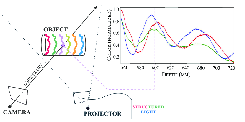
Figure 2. Schematic of LookUp reconstruction. A projector illuminates the scene with a specific structured light pattern $P_{i}$, whereas we highlight a single camera array in the scene. We search for the closest color in L2-norm for each camera ray to identify its depth.

The goal of our calibration is to acquire a complete volume of normalized colors for each pattern $P_{k}$. That is, we want to find a per-ray and per-pattern 1D function $C^{i,j}_{P_{n}}(d)$ storing the normalized intensity that an object placed at $d$ distance on the ray would have if the pattern $P_{n}$ is projected.

Normalized Intensity.

To factor out object texture and lens vignetting we normalize the color at each pixel (Caspi et al., 1998) against a projected white image (Figure 3). For each series of projected patterns $P_{k}$, we always add a full white pattern $P_{W}$ (ambient light is subtracted beforehand). We denote as $I_{P_{k}}(i,j)$ the image acquired by the camera with the pattern $P_{k}$. We define the normalized color image as (see Figure 3 for example):

(1) $$\tilde{I}_{P_{k}}(i,j)=I_{P_{k}}(i,j)/I_{P_{W}}(i,j).$$

/ =

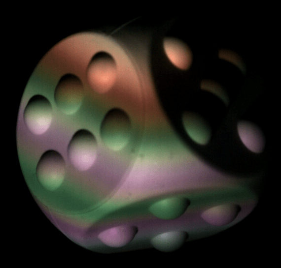
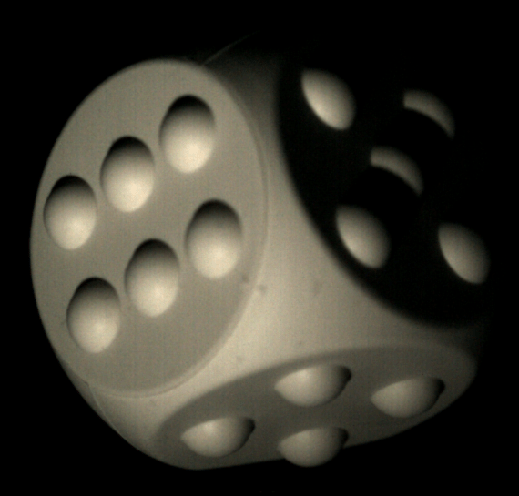
Figure 3. Normalized colors (right) are obtained by dividing each pixel of an image acquired while projecting a pattern (left) with the corresponding pixel of an image obtained by projecting white (middle).

Acquisition.

To perform these measurements, we propose an active calibration hardware composed of an off-the-shelf motorized linear stage and a custom calibration board (Figure 1, left). The calibration board is fabricated using an aluminum honeycomb and is assumed to be flat, a reasonable assumption given that the fabrication tolerance is negligible compared to our target resolution. The pattern on the calibration board is a custom pattern with ChArUco tiles on the boundary and uniform white in the center. During calibration, the pattern is moved in a linear trajectory, stopped every 150 microns, and a stack of images (one for each input pattern $P_{k}$ plus one for the white pattern $P_{W}$) is acquired with the camera while the patterns are projected. We note that if using a color camera and projector it is possible to pack up to 3 patterns in a single image by using the three color channels. The board’s position is reconstructed in each frame relying on the ChArUco tiles using OpenCV. The reference frame of each board plane is then least-square fitted to a linear trajectory (exploiting the fact that the linear stage fabrication tolerances are low) to further reduce measurement errors.

Spline Fitting.

This procedure provides us with a set of measurements on each camera ray, one for each intersection between a calibration board and the ray. To obtain a smooth per-ray color function, we fit a 1D cubic B-spline. The spline fitting is done using the function scipy.interpolate.splrep in SciPy. We note that the fitting is done independently for each projected pattern. After fitting, the calibration data can be discarded: the output of this stage is a set of 1D splines, one for each pixel of the camera and each pattern.

3.2. Scanning and Reconstruction

The scanning procedure is identical to calibration: the patterns are projected in sequence, and the corresponding images are acquired and normalized against the projected white pattern, leading to a stack of normalized images $\tilde{I}_{P_{n}}(i,j)$. The reconstruction is embarrassingly parallel and done independently on each pixel $(i,j)$. For convenience, we define $c=(\tilde{I}_{P_{1}}(i,j),...,\tilde{I}_{P_{n}}(i,j))$ as the $n$-vector stacking the intensity for the pixel $(i,j)$ of all acquired images, and $C(d):R\rightarrow R^{n}$ the multivariate function returning the stacked intensity of all calibration rays corresponding to the pixel $(i,j)$: $C(d)=(C^{i,j}_{P_{1}}(d),...,C^{i,j}_{P_{n}}(d)).$

The reconstruction algorithm is a lookup on the ray to find the color closest to the one acquired:

(2) $$x=\operatorname*{arg\,min}_{d}|C(d)-c|_{2}^{2}.$$

Implementation.

The algorithm is implemented by sampling with a spacing of 10 microns for each ray, and performing a brute-force search to find the color with the smaller L2 distance.

Discussion.

A key assumption for our algorithm to reliably construct depth is that each depth value in a ray should have a corresponding distinct color to ensure that the lookup is unique. This is, in general, very difficult to achieve, and figuring out which pattern gets closer to this idealized desiderata is a challenging and interesting problem. Since we do not want to change the projector or the camera focus for different depths, the acquired color will depend not only on the pattern but also on how the projector and the camera blur and distort it.

We will first discuss how to design and evaluate patterns (Section 4), and then study how our method compares to alternatives in static (Section 5) and dynamic (Section 6) settings.

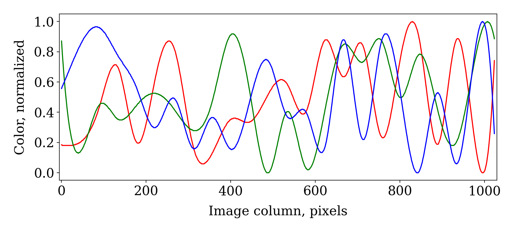
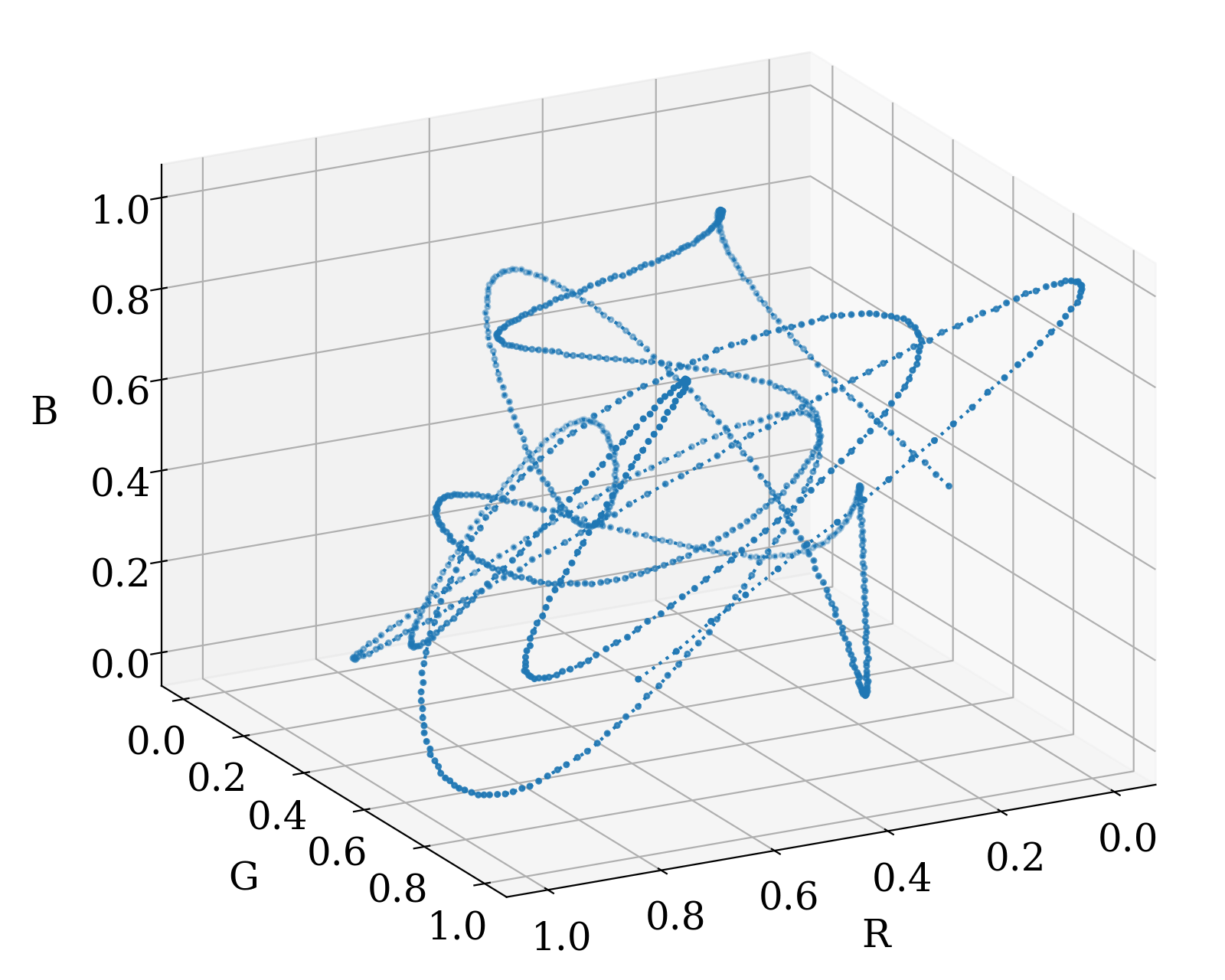
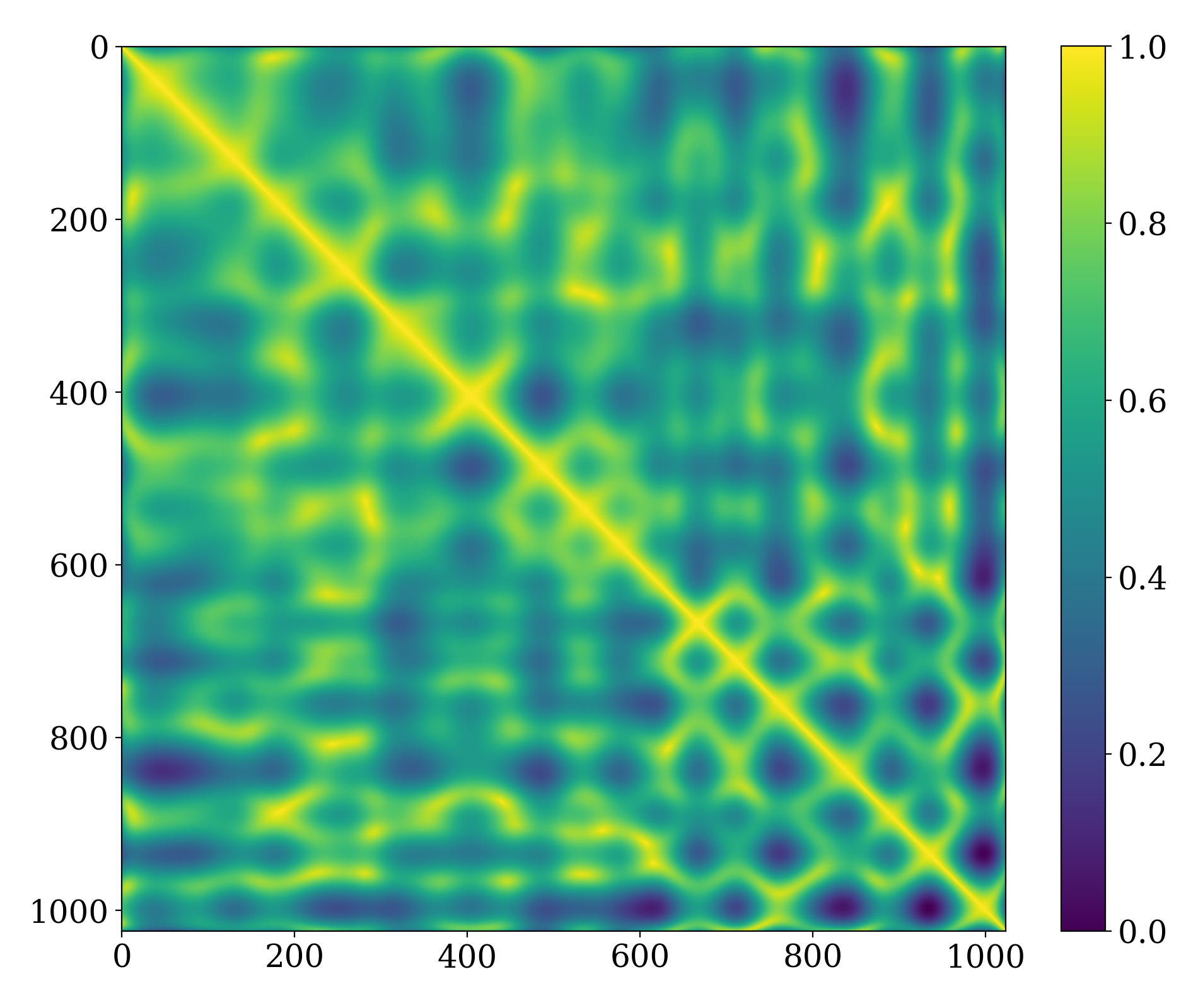
(a) Random

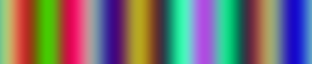
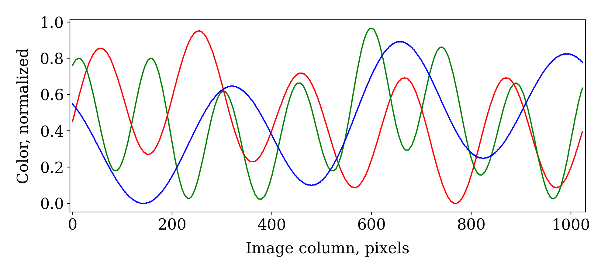
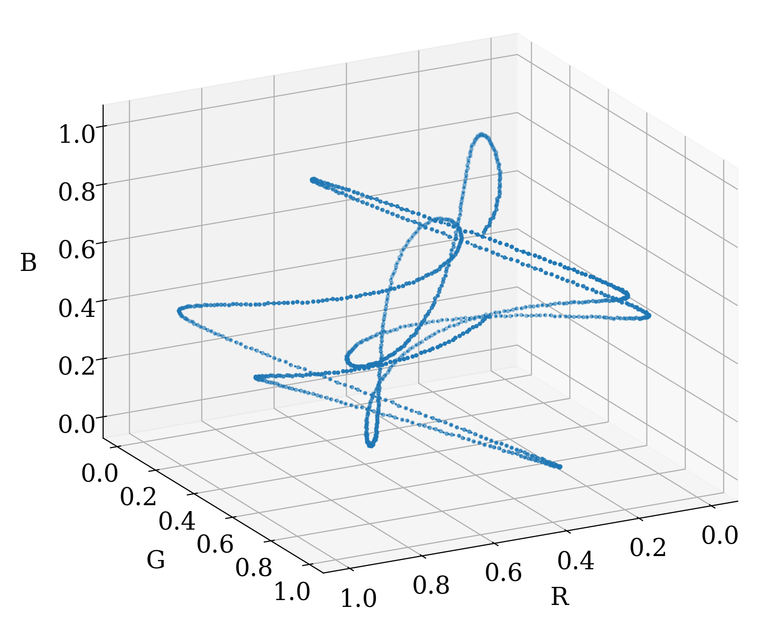
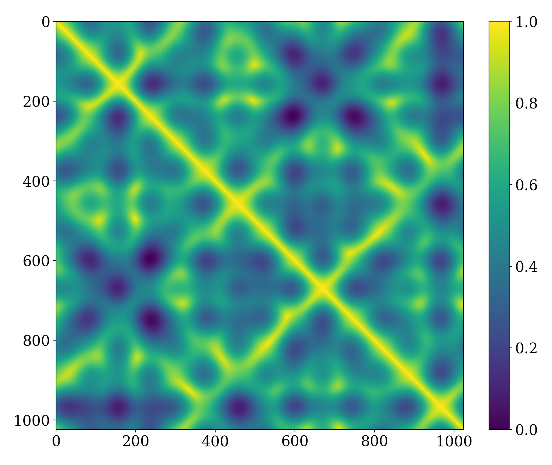
(b) Lissajous

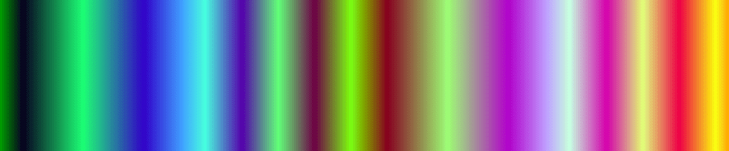
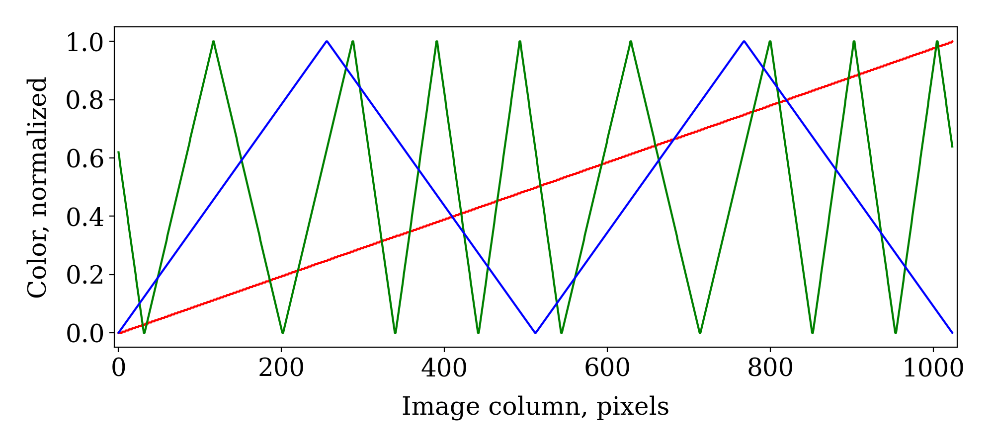
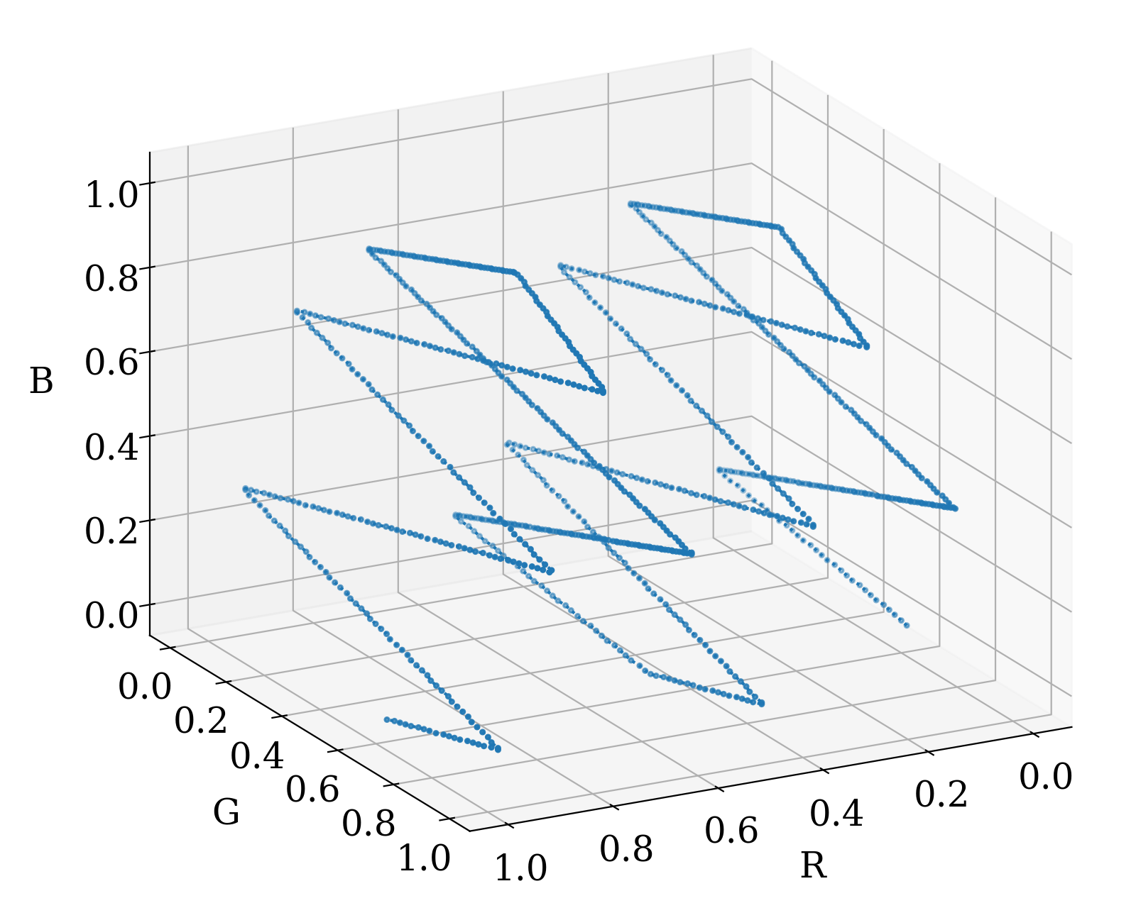
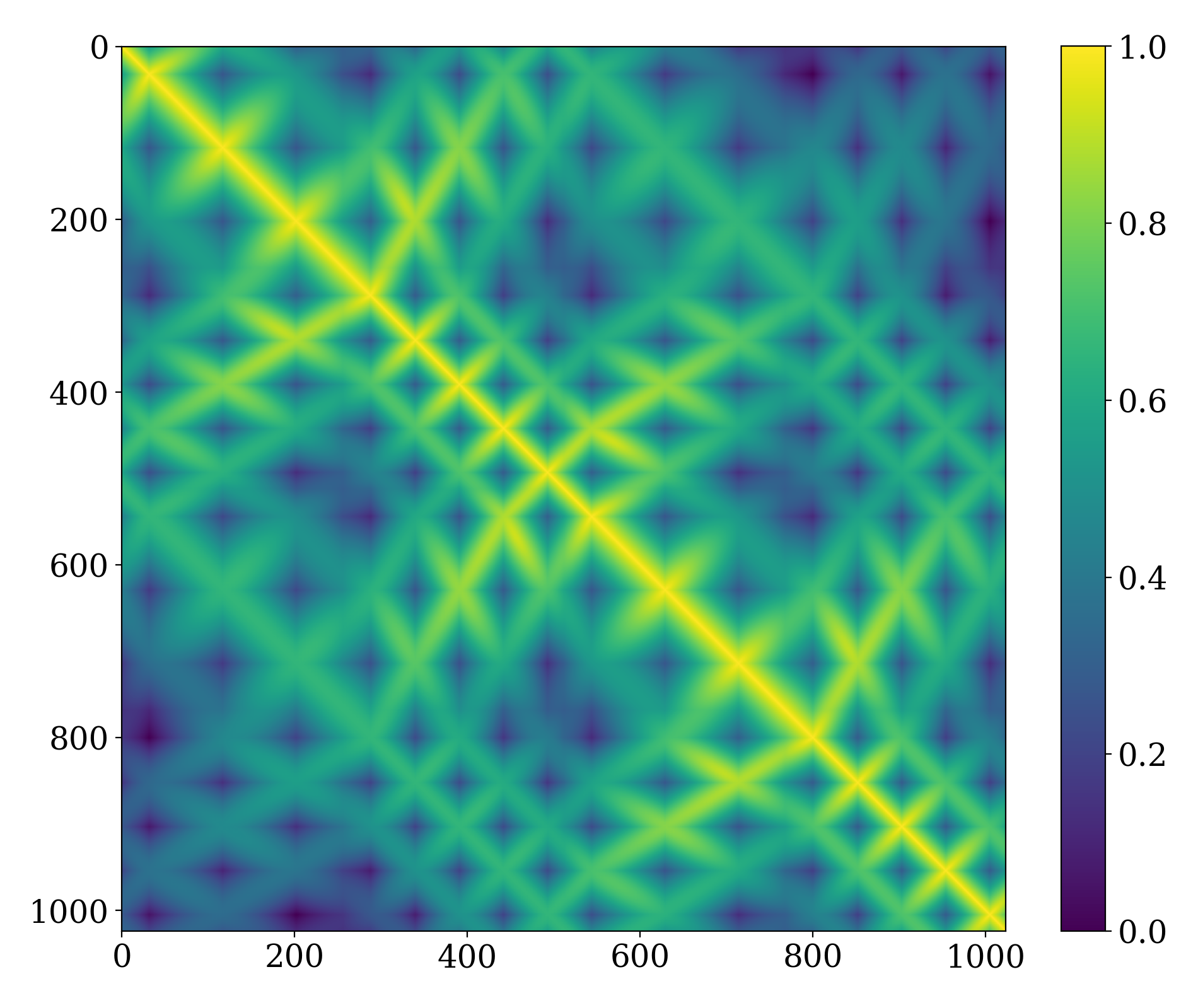
(c) Stairs

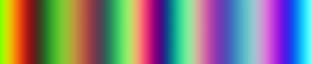
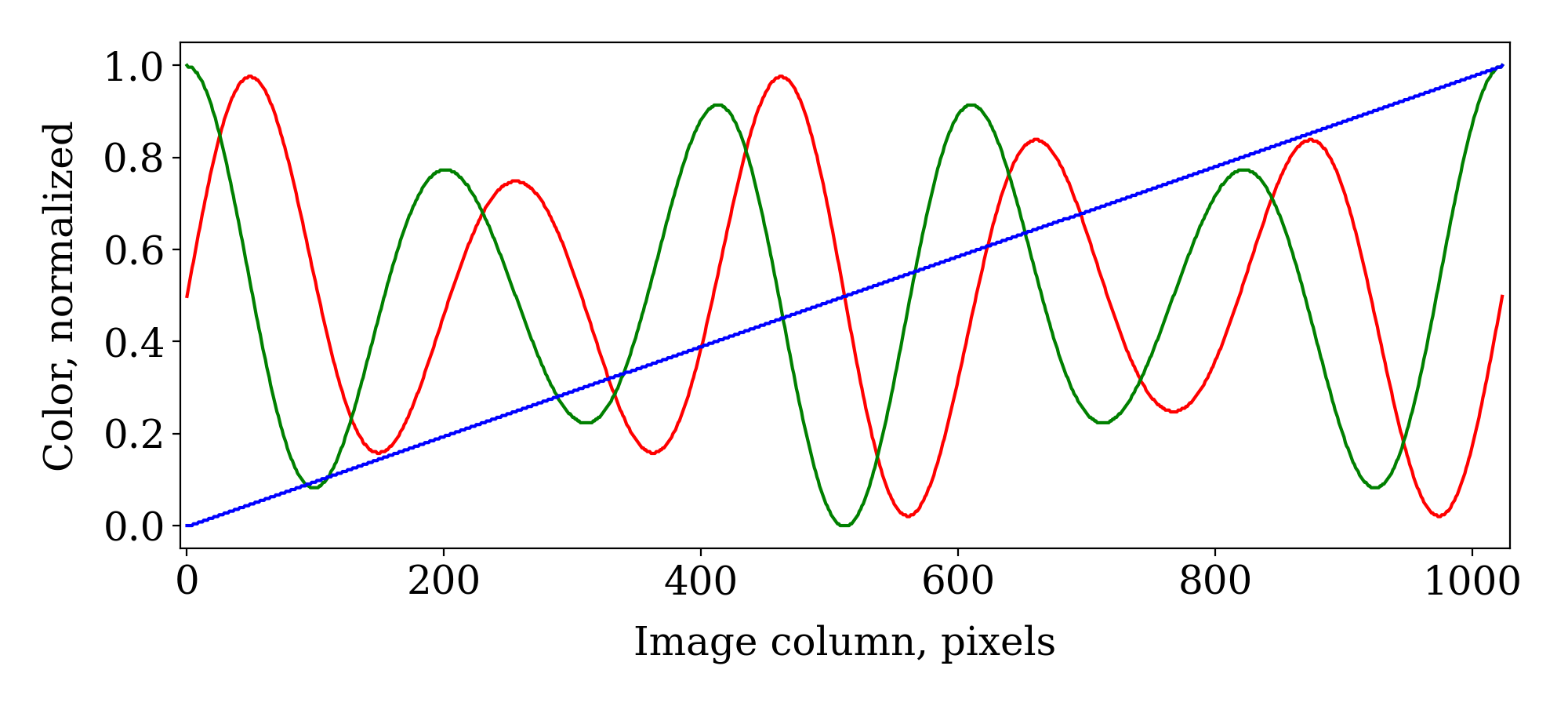
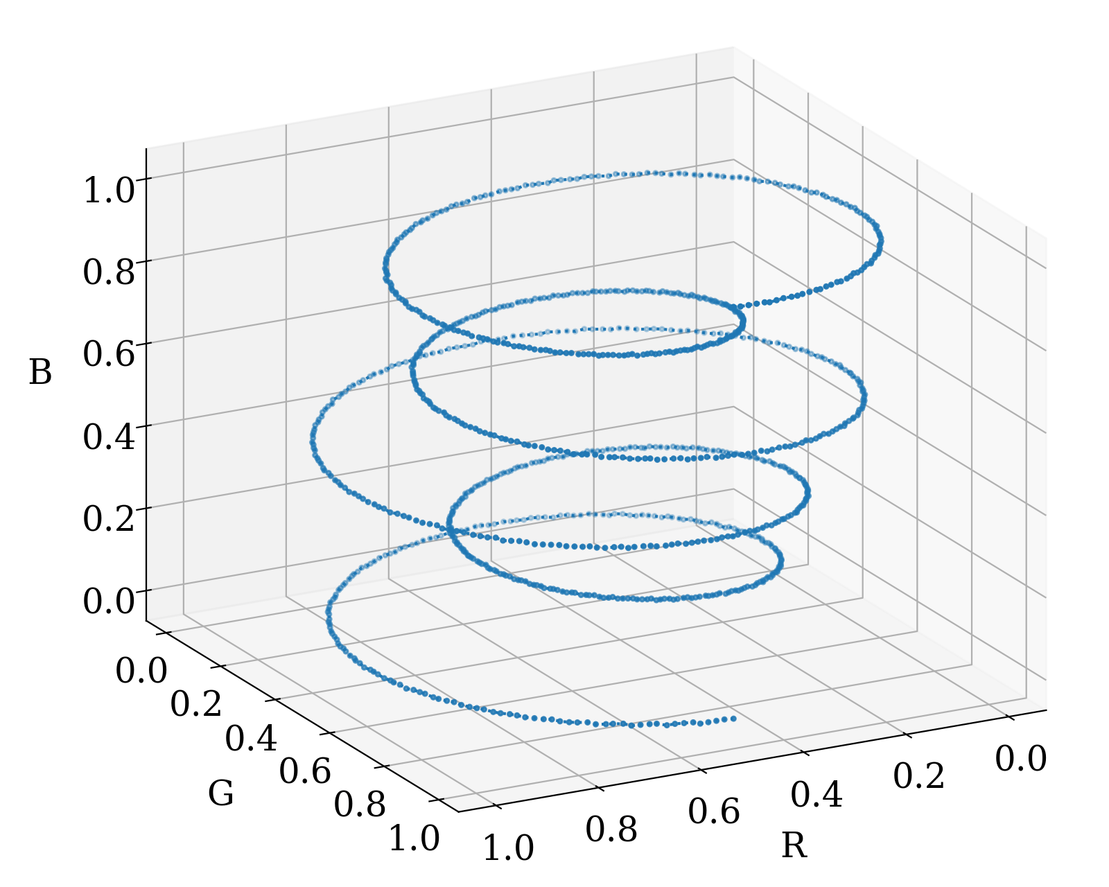
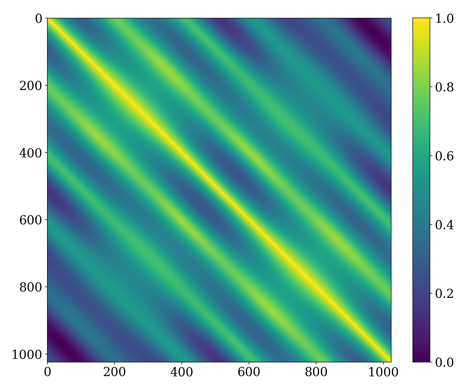
(d) Spiral

Figure 4. A comparison of different RGB patterns tested. Note that the patterns visualized here use a lower frequency than what we use in the hardware setup for presentation purposes. The confusion matrices are normalized on per pattern basis to better represent the confusion structure within each pattern.

4. Pattern Design

Pattern design has a huge impact on our ability to estimate the depth from the acquired intensities. Designing pattern sequences is a delicate balance: the use of many patterns makes the depth values easier to differentiate and makes the reconstruction more resilient to noise and at the same time increases the time required for acquisition. While for static scanning this is not an issue, for dynamic scanners the use of many patterns negatively affects the acquisition speed and also makes the acquisition of fast objects more noisy, as they will look different as the system cycles through the different patterns. Our focus in this section is to analyze pattern types, and their effect on our ability to differentiate depth, under the strong restriction of using only 3 monochrome patterns (plus the white one for normalization, see Figure 3), which can be stacked into a single RGB image.

Information Transfer.

Structured light 3D scanning can be viewed as an information transfer problem. For instance, when the scene illuminated by a structured light is imaged with a monochrome camera, there are typically ~12 bits of dynamic range for the light intensity information captured by the camera for each pixel. Ideally, in a world with no camera sensor noise or distortions, that would allow one to decode $2^{12}=4096$ possible depth locations where the scanned object might be along said camera ray. Realistically, a few least significant bits will most likely be too noisy to be useful and a few most significant bits need to be reserved to account for the dynamic range of object illumination/texture, leaving us with a couple hundred depth gradations at most which would be insufficient for a high-quality reconstruction.

An obvious way to improve the situation is to use multiple readings, i.e. use multiple monochrome patterns. Acquiring the patterns sequentially is a great choice for static scanning but has a negative impact on acquisition speed. We can however trade spatial resolution for additional dynamic range by using a color Bayer filter on top of the sensors. In this way, we can acquire 3 monochromatic patterns in one image, at a quarter of the image resolution: we are effectively trading one bit of spatial resolution in order to triple the amount of information captured for each pixel. This makes it much more feasible to perform reliable scanning with more than a thousand depth gradations for each pixel even in the presence of image noise and specular materials.

Revisiting Section 2 with this information transfer angle, we observe that existing structured light papers use different patterns to encode the projector plane, which is then intersected with a camera ray. We go one step further and propose to directly encode the per-ray depth, and we study patterns that are optimal for this purpose.

4.1. Monochrome Pattern Types

There are many monochrome patterns explored in prior work and we would like to highlight the major types.

Binary Patterns.

Binary patterns, such as ubiquitous gray code patterns (Inokuchi et al., 1984), are very robust to noise and textures by using the entire intensity range (12 bits) to encode only 1 bit of depth information. This makes thresholding very reliable, especially when the lighting conditions cannot be controlled. This is however very inefficient: it is usually necessary to use $\log_{2}(\sqrt{r})$ patterns where $r$ is the image resolution, leading to a sequence of ~11 patterns for 1 MP.

Linear Intensity.

A linear ramp is used in the intensity ratio method (Carrihill and Hummel, 1985). This pattern is very imprecise (close depths have very similar intensity values) but uses the full dynamic range. It also requires a linear response from both the projector and the camera, which is very hard to achieve, even after calibration. It is common to normalize this ramp with a white image to take relative measurements instead of absolute ones.

Phase Shifting.

A third group of patterns is smooth by design and consists of multiple sine waves of different frequencies and amplitudes. These patterns have a property of having constant precision, meaning that if two or more patterns are used, at any point on the domain there is at least one pattern that has a non-zero gradient. This is useful, as it implies that at least one of the channels is resilient to noise everywhere on the domain.

4.2. RGB Patterns

We use three different visualizations to compare different patterns to better understand their performance. Note that we use patterns made of stripes as they are easier to use in a physical setup: to maximize their effectiveness we want the stripes to be as parallel as possible to the plane perpendicular to the camera rays (i.e. the 1d color pattern is mapped to the ray). This is just a practical convenience to make it easy to align the projector in a physical setup, our reconstruction method does not require or use this structure.

In Figure 4, we show four of our designs in the form of an RGB image (1st row), the intensity plots of individual channels (2nd row), the plot of the pattern in a space where the three coordinates are mapped to colors (3rd row), and finally as a confusion matrix (4th row), where a pixel $i,j$ has the value of the L2 difference between the color at depth $i$ and $j$. The goal is to get maximal separation. In the 3rd row, we want the curve to span the space without getting too close to itself, i.e. if points on the curve are far, they should be far in space too. In the 4th row, we would like to see a single bright diagonal, which denotes minimal confusion. An important technical note is that the three channels are not symmetric: due to the Bayer pattern, the green channel has less noise than the other two, and we thus always place the signal of higher frequency on that channel.

We tested 4 different designs (Figure 4):

1. the Random pattern is generated by sampling random colors and interpolating them with a cubic B-spline with uniform knots. This pattern has the worst performance judging by the line plot, with the curve almost intersecting in multiple regions, and the bright confusion matrix.

2. the Lissajous pattern inspired by the Lissajous (also known as the Bowditch curve (Anon, 2023b)) is superior to the random pattern, as the curve "threads" more uniformly.

3. the Stairs pattern uses linear ramps at different frequencies. Disappointingly, the space coverage is still not ideal, in addition to introducing color discontinuities which are difficult to fabricate and will be lost due to camera and projector blur.

4. the Spiral pattern combines the Lissajous and Stairs patterns. It uses a linear ramp and a pair of sine and cosine patterns with modulated amplitude to further reduce similarities.

Judging by the confusion matrices for each pattern (bottom row in Figure 4), it is clear that the Spiral is the most favorable design in our set: it has a consistently lower confusion score the farther away we move along the pattern thanks to the sampling of the color cube space (middle row in Figure 4) with maximized distances between consecutive turns. It would be interesting to apply an optimization method to further optimize the pattern for a given color response of both camera and projector: we however leave this as a future work.

5. Static Analysis and Experiments

To evaluate the effect of our calibration and reconstruction method in isolation, we built the state-of-the-art structured light scanner proposed in (Koch et al., 2021) and used their software for calibration and reconstruction. We then compare the reconstructions obtained using their method, which is a very accurate triangulation-based structure light approach with gray code patterns, with ours.

5.1. Qualitative Comparison

First, we use a pawn figure coated with white specular paint to investigate when and how each method/pattern combination behaves for a specular material (Figure 5). We highlight three key differences.

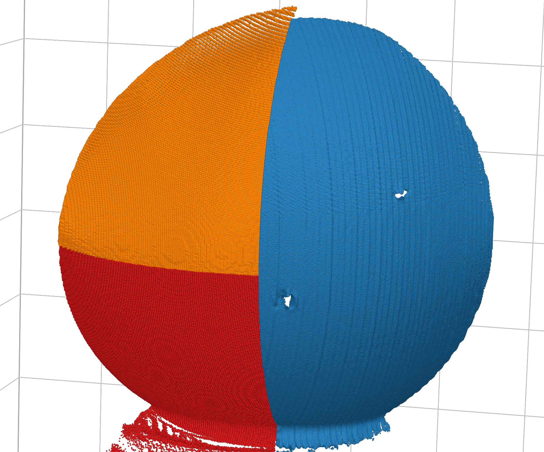
(a) Triang. vs. LookUp

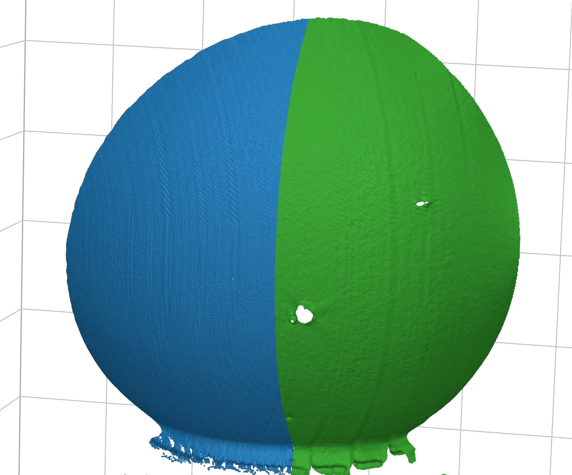
(b) Gray vs. Colors

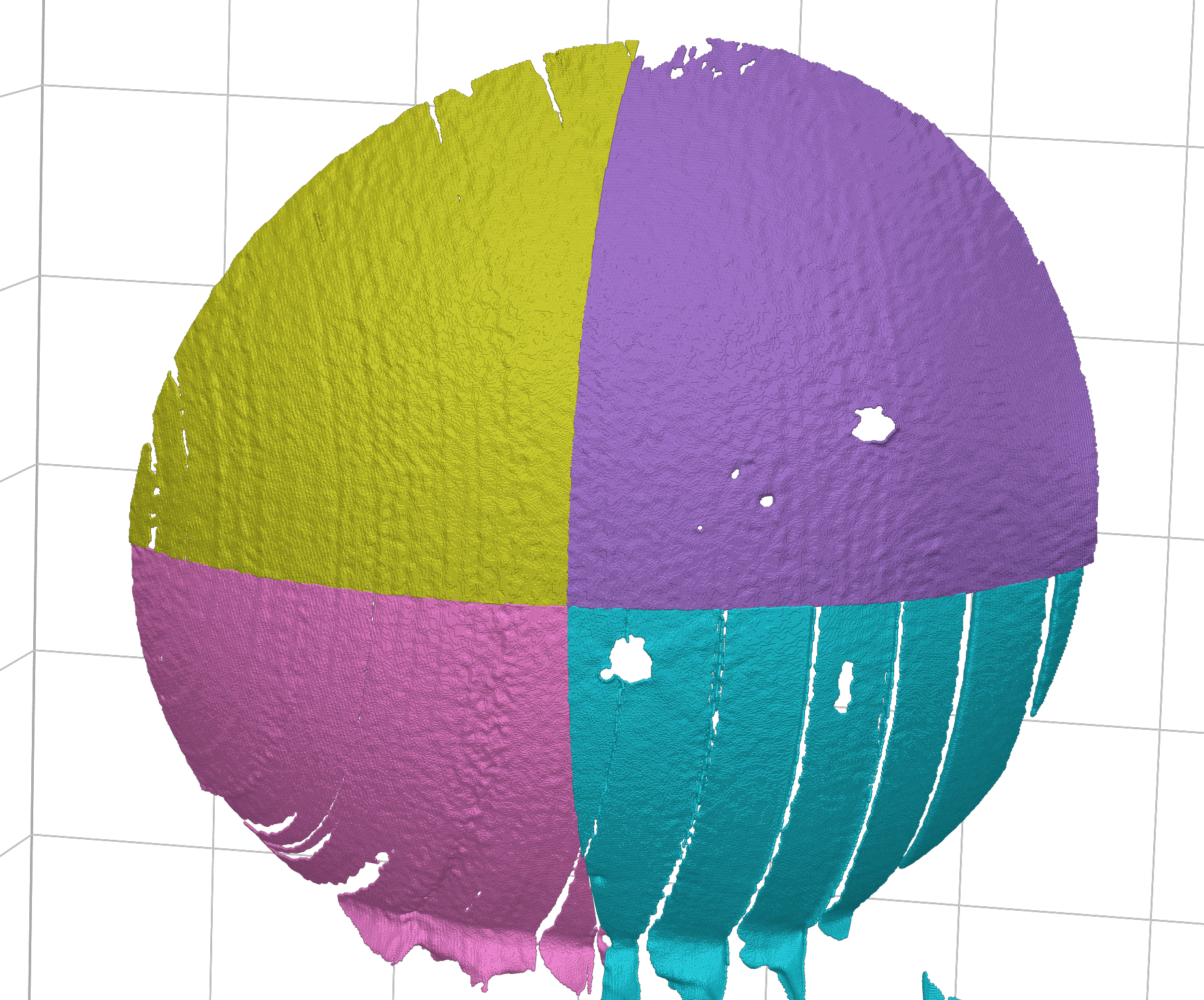
(c) RGB Patterns

Figure 5. Qualitative comparison of pawn reconstructions. We plot the pawn head in the same position and camera view using different reconstruction methods, each represented by a unique color. Red: Triangulation; orange: Triangulation+ with the grouping of camera rays; blue: LookUp3D Gray; green: LookUp3D Colors; olive: Lissajous Pattern; pink: Random Pattern; cyan: Stairs Pattern; purple: Spiral Pattern.

Triangulation vs. LookUp3D, Gray Code Patterns.

Figure 5(a) (left) shows a triangulation-based reconstruction using gray code patterns with (bottom-left) and without (top-left) grouping of camera rays corresponding to the same projector rays. This is a refinement stage implemented by (Koch et al., 2021) that accounts for the camera’s resolution being higher than that of the projector, and it yields cleaner point clouds but with distinct discretization of the object’s surface (we refer to it as Triangulation+). Our LookUp3D method, in contrast, offers smooth point clouds at the full resolution of the camera instead of being bound by the projector resolution (Figure 5(a), right). A downside of our approach is that it is more sensitive to the specularities, which are captured as bumps on the object’s surface. We note that due to memory limitations, our method uses only one-quarter of the patterns used by the triangulation method (we use vertical stripes only without inverse images).

Single RGB Pattern.

Next, we look at three monochrome patterns stacked into a single RGB image. Figure 5(c) shows the split-rendered comparison of reconstructions with the LookUp method using four different RGB patterns (see Section 4). We want to highlight that the Lissajous and Spiral perform best thanks to their "constant precision" smooth design. Random pattern, as expected, has issues in random locations due to color confusion at different depths. Similarly, the Stairs pattern is a non-smooth attempt at constructing a constant precision pattern and suffers from loss of precision at regular intervals when its high-frequency component has a rapid change in the gradient direction (Figure 4(c)).

Gray vs. Colors.

Finally, we compare, in both cases using our algorithm, a standard stack of 11 gray code patterns against a stack of 16 monochrome patterns, grouped into 4 RGB images. The performance of the color patterns is superior due to their smooth design, making it a better choice than the gray code patterns.

5.2. Quantitative Comparison

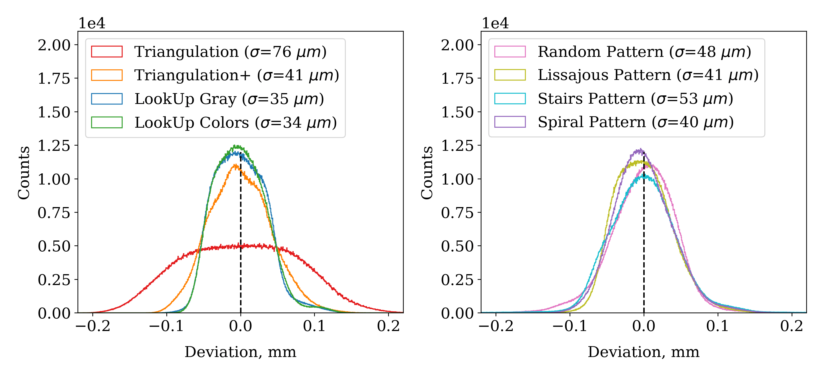
Figure 6. Principal Component Analysis of a flat plane. We attempt to reconstruct a smooth, flat plane with our two different methods: triangulation and lookup (with gray and RGB patterns). The histograms show the count of deviation (in millimeters) of each reconstructed point when compared to a perfectly flat surface.

We estimate the reconstruction noise for different method/pattern combinations by scanning a flat-plane object. We then perform PCA analysis on the cropped portion of the said plane to obtain the standard deviation of the reconstructed points from the fitted plane (see Figure 6). The baseline triangulation method performed the worst with a standard deviation of $\approx 75\mu m$. The refining stage of (Koch et al., 2021) almost halves this number to $\approx 40\mu m$. Our method has slightly better performance, with $\sigma\approx 35\mu m$ regardless of the patterns stack used. Also, the Random and Staircase patterns performed the worst among RGB patterns ($\sigma\approx 50\mu m$) with Lissajous and Spiral patterns offering the same degree of precision as the Triangulation+ method but with a single image ($\sigma\approx 40\mu m$).

6. Dynamic Analysis and Experiments

With our approach, scanning at $x$ fps requires a synchronized camera and projector able to capture/project at $2x$ fps: the projector will alternate projecting the Spiral pattern and a white pattern for normalization. While off-the-shelves high-framerate cameras are available (iPhones can do 240 fps, and the Chronos HD camera we use can do 1k fps), the same is not true for projectors. The best color projectors we could find off-the-shelves are based on DPL technology and max out at 120fps.

6.1. Analog Projector

We propose an effective alternative: a purely analog projector that can project the two alternating patterns at over 1k fps and at high resolution. We show a diagram of our projector in Figure 7. It comprises two high power (100 Watt) LEDs $L_{front}$ and $L_{side}$ illuminating the corresponding diffusers, which are located at 90 degrees angle to each other. A 35-mm color film slide with the color pattern exposed onto it is placed in front of one of the diffusers and a light trap against another with a beam splitter in between. The LEDs are individually controlled with power transistors and a microcontroller, which also triggers the camera in sync with the projector. This way, we can alternate between the color pattern and white at frequencies greater than 1 kHz. We are using a Chronos 2.1 Full HD camera with a Sigma 35mm f1.4 that can record bursts of frames at 1k fps. The projector uses a Sigma 50mm f1.4 lens. To expose the film, we use a calibrated static 4k projector, and a Canon A1 analog camera with a Tamron 90mm f/2.8 lens. To ensure reproducibility, we provide a CAD file for the analog projector design in the additional material, and we plan to keep in storage pre-exposed 35mm film slides with the Spiral pattern to ship to the research lab interested in reproducing our setup (as this is the only custom part used in the projector and it is easy for us to produce in sufficient quantities).

We note that this analog projector design can only be used with our method and using a single pattern: it would be very challenging to add additional patterns to this setup, as it will require additional beam splitters, higher power light sources, careful alignment, and additional lenses. We designed our pattern and algorithm specifically with this hardware solution in mind.

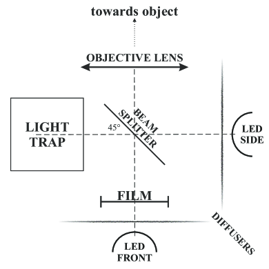
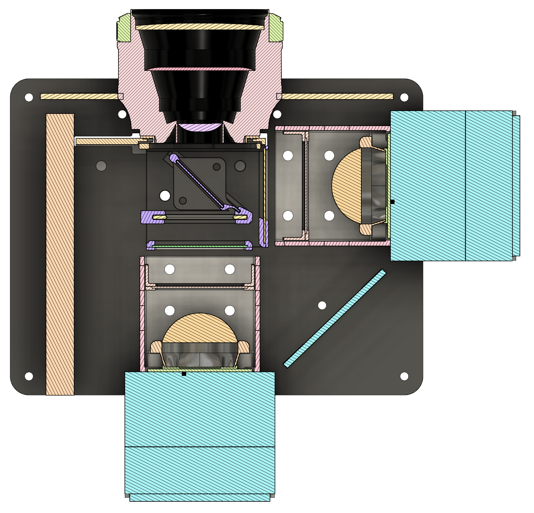
Figure 7. Schematic of a specialized analog projector (left) used for high-speed 3D scanning with alternating color and white patterns. The corresponding cross-section of the projector’s CAD model is shown on the right.

6.2. High FPS

For high-speed capture, we configure the camera and the projector to use 1.25 ms exposure for the pattern frame and 1 ms for white. This is done to compensate for the fact that the film does not transmit the light perfectly (part of it gets inevitably absorbed by the substrate) and, thus, boost the signal-to-noise ratio during color normalization. This results in a scanning speed of 400 pattern pairs per second, which we will refer to as 400 fps. Figure 10 (top row) shows a progression of a dynamic scene where a silicon dice-shaped cube falls and bounces off an air balloon, causing it to squish and bounce off in the opposite direction. The entire action ($T_{2}-T_{0}$) took 38 ms, i.e. a single frame at video speed (26 fps). Of note is the partial detection of the falling cube before ($T_{0}$) and after ($T_{2}$) the still moment $T_{1}$. This is due to the increased noise/error during its reconstruction because of the motion blur of the pattern frame, leading to depth bias/confusion, and so some points do not pass the temporal filtering stage. The filtering is implemented as a basic moving average on three consecutive frames with an additional condition on points not differing in depth by more than 1 cm from frame to frame.

6.3. Low FPS

We compare our high-speed scanner prototype with three commercial depth sensing devices: Photoneo MotionCAM 3D M+, Intel Realsense 455, and Microsoft Azure Kinect (bottom row in Figure 10). We, unfortunately, cannot compare on the exact same scene, as all three scanners use infrared and do interfere with each other if used at the same time. We thus repeat each scene for each scanner, striving to keep the initial conditions as similar as possible. We note that there is a very high discrepancy in the framerate of the scanners (8fps Photoneo, 90fps RealSense, 30fps Azure Kinect) compared to 400 fps for ours.

Photoneo. Photoneo offers the most "clean" point clouds at high resolution but a very low frame rate (8 fps). Also, fast-moving objects are not captured at all. RealSense. RealSense has the highest frame rate (90 fps), but this is compensated by a low resolution and the point cloud tends to blur/smooth out a lot for fast-moving objects. Azure Kinect. Kinect strikes a balance between the previous two scanners in terms of scanning speed and resolution. However, fast-moving and even static objects tend to fuse with each other or their background. LookUp3D. Our scanner, in contrast, compromises on neither speed of scanning nor point cloud resolution.

Our hardware prototype has one main limitation: the 35mm film limits the power of the LEDs we can use as increasing the power further will lead to too much heat (even with our active cooling system) that would melt the film. The current 100W power is plentiful for low fps, but it is the limiting factor at 400 fps, resulting in more image noise. This limitation could be lifted with additional hardware engineering, for example using a large format film. To better understand the advantages and limitations of our analog setup without this limiting factor, we perform an additional analysis of the performance of our analog scanner when used on static objects (Figure 8).

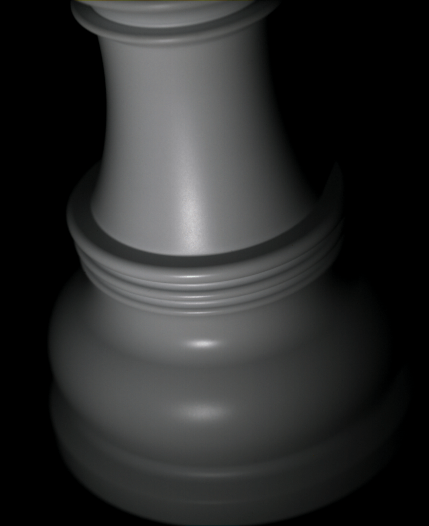
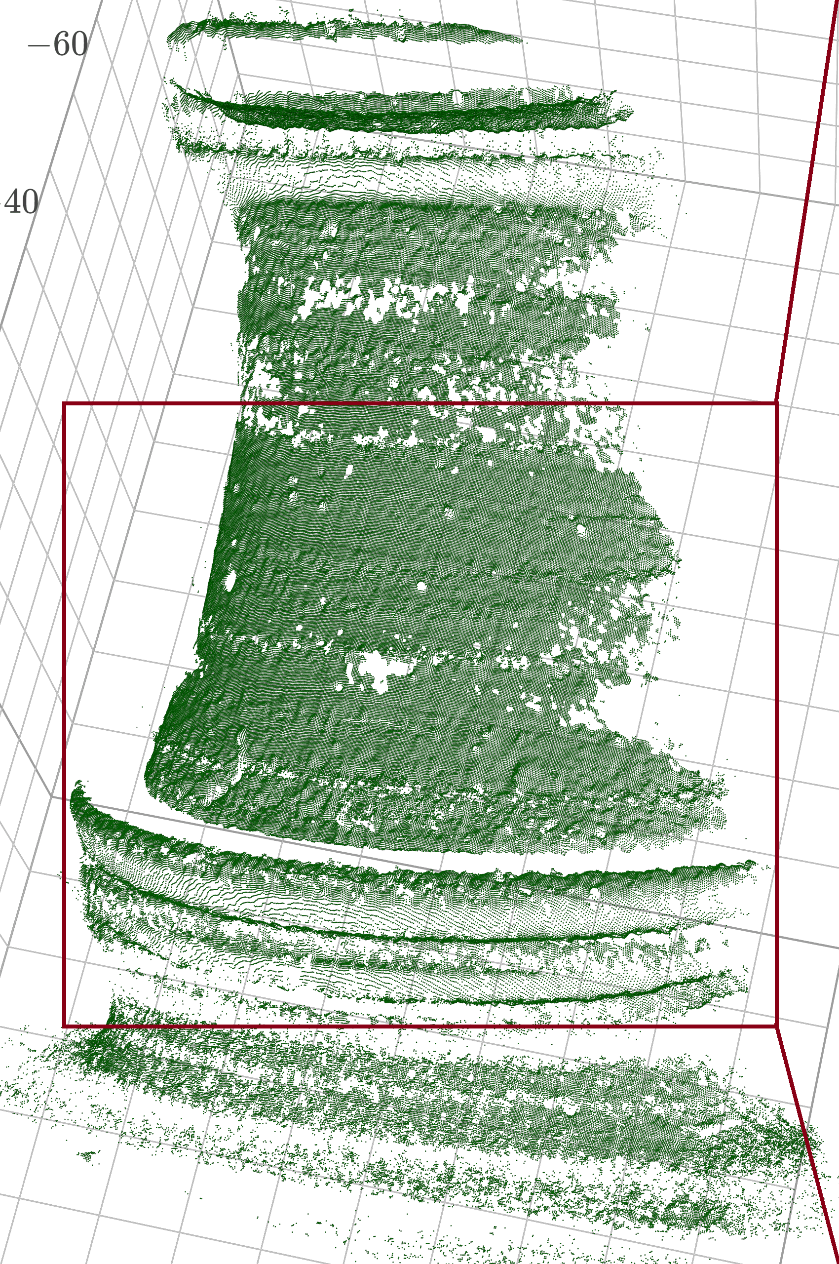
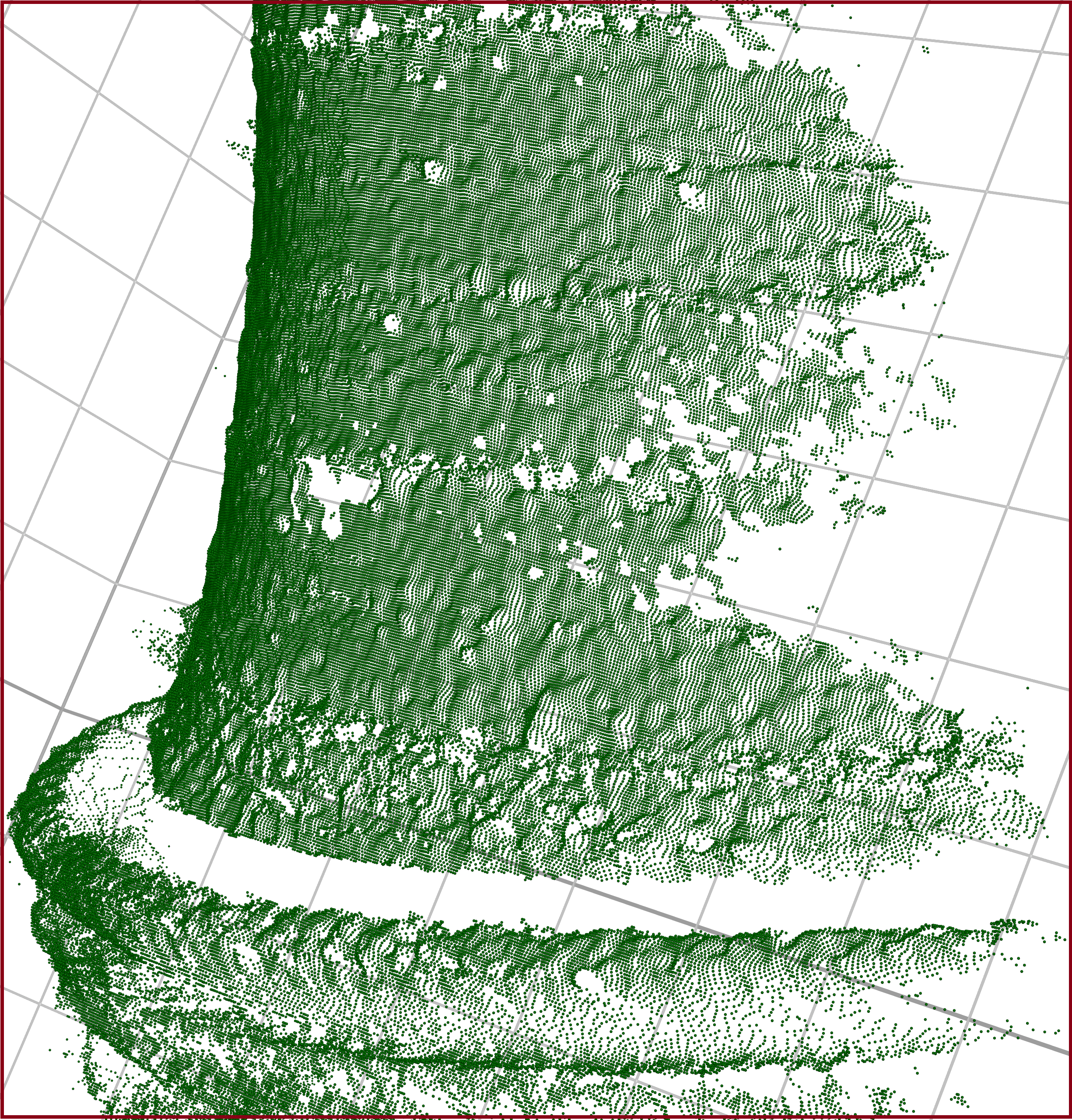
Figure 8. Rook under white pattern illumination (left), its static reconstruction (middle), and a zoomed picture into the reconstructed shelf (right). This model is acquired with our analog projector, averaging ten frames to mimic how a dynamic reconstruction would look with a brighter projector.

7. Concluding Remarks

The major limitation of our approach is the limited brightness of our analog projector, which is the limiting factor in achieving higher framerates: we believe with different projector designs, which are possible thanks to the simplicity of projecting a single pattern, it will be eventually possible to acquire depth data of similar quality as our static scans but for dynamic scenes. We note that there is only one difference between our static and dynamic results, the exposure time of the projector and the camera, which directly affects sensor noise and reconstruction errors.

The possibility of using arbitrary patterns with the LookUp3D reconstruction algorithm opens many interesting avenues for future work: (1) it is possible to use multiple synchronized projectors and cameras to increase scanning view without worrying about interference (as long as the projectors do not overexpose), (2) the use of multiple analog projectors multiplexed in time to reduce noise at the cost of lower temporal resolution, (3) the use of invisible light patterns (infrared) potentially combined with visible light, and (4) alternatives to the use of a film in the analog project to support higher-power projectors.

We are excited to explore applications of our new hardware to acquire reference geometry for deformable objects in high-speed contact scenarios, and in robotic state estimation for soft object manipulation. However, this will require major improvements to our reconstruction efficiency, which is still not real-time, especially at higher fps. This could be achieved by either developing GPU/TPU accelerations or finding ways to compress our calibration data, for example, using neural networks.

Appendix A Figures

A.1. Static Objects

Please see Figure 9 for a comparison of the static object reconstruction using different patterns/methods in the digital setup.

A.2. Dynamic Scenes

Please see Figures 10 and 11 for a comparison of the dynamic scenes captured using our analog setup and three commercial scanners.

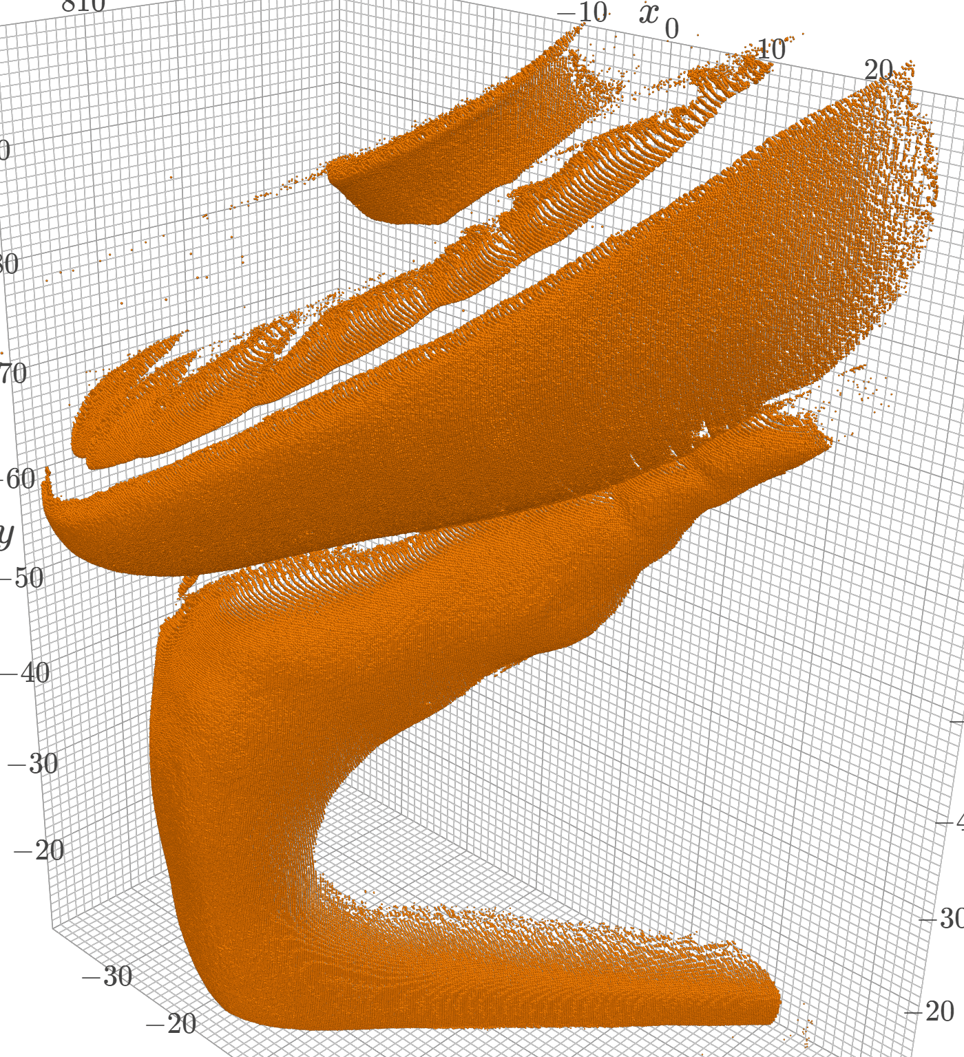
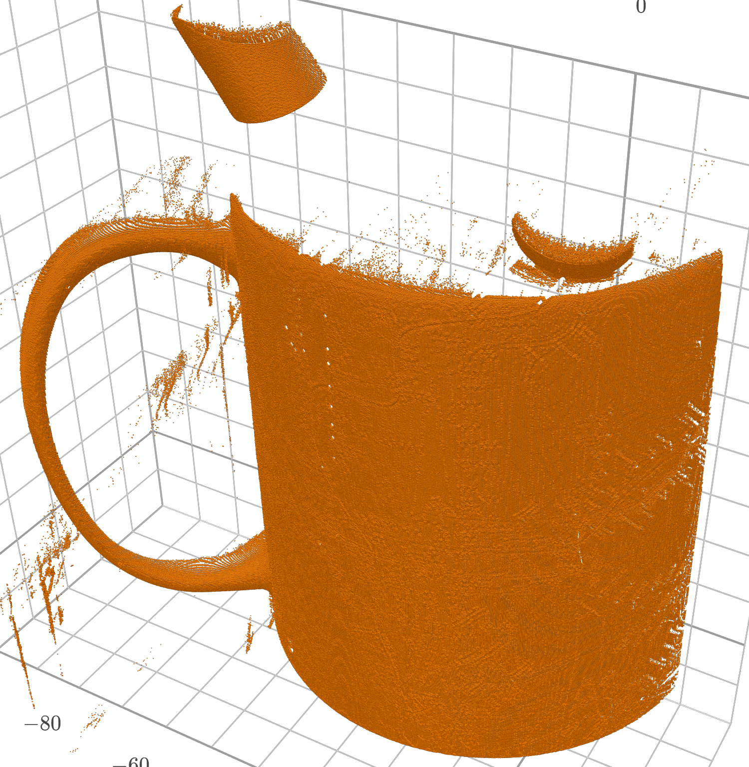
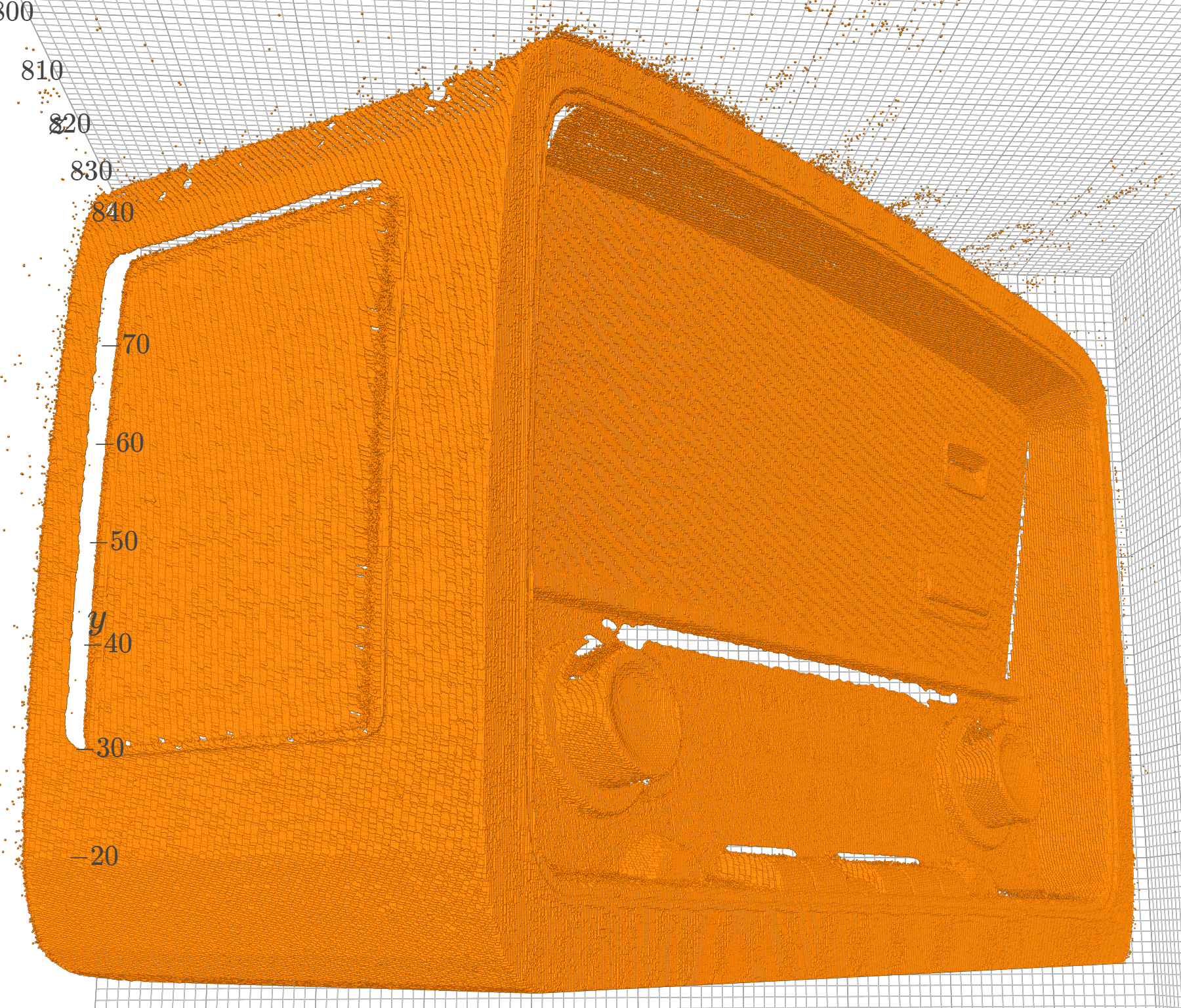
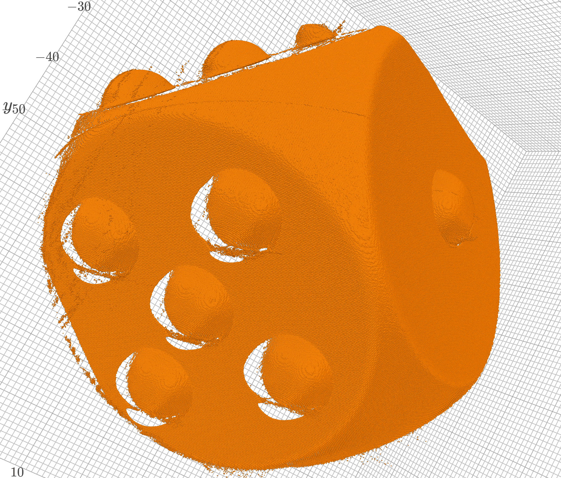
(a) Triangulation+

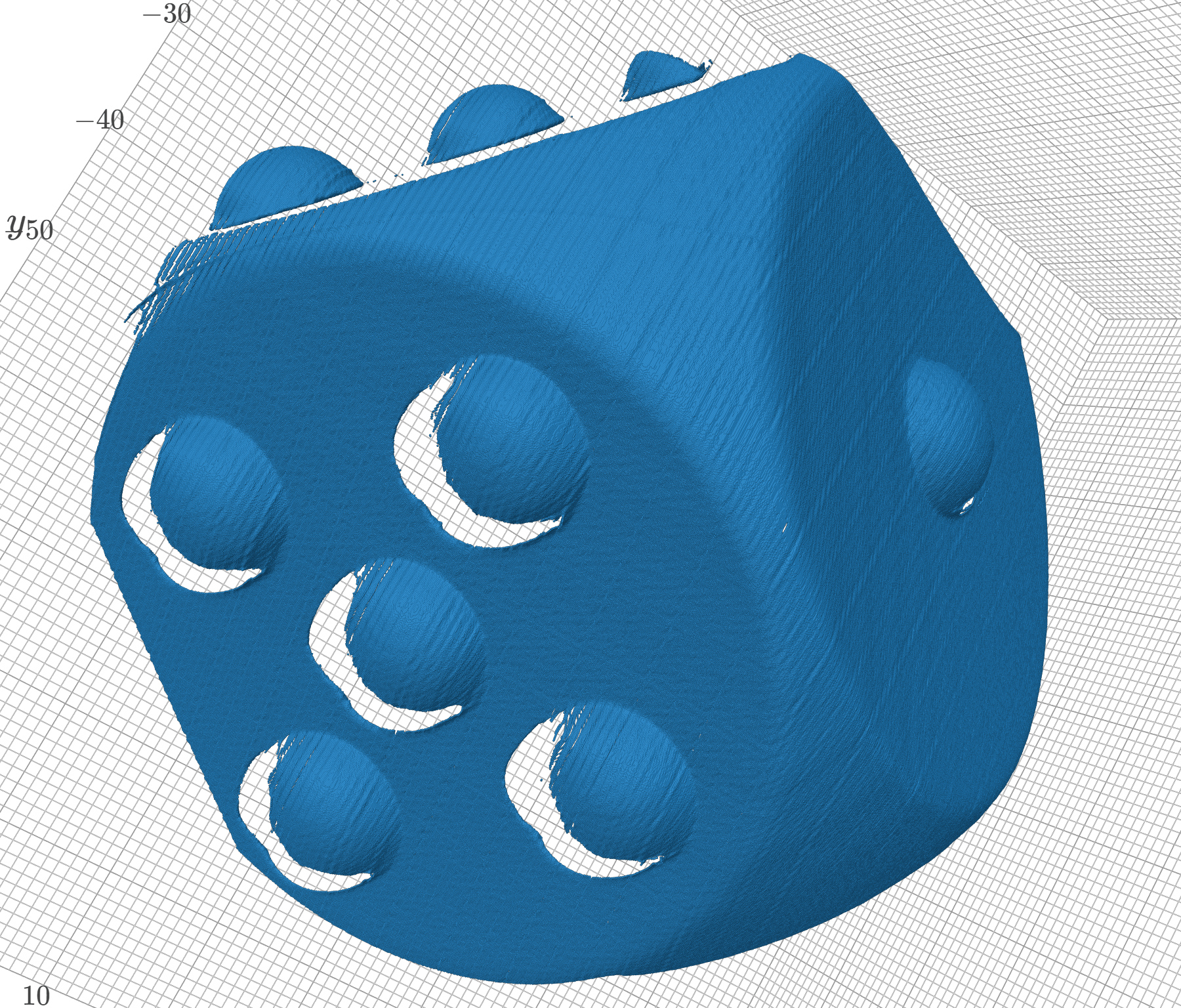
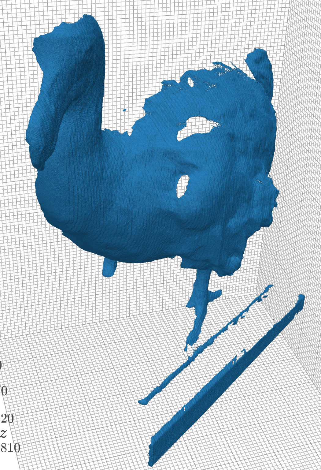
(b) Gray LookUp3D

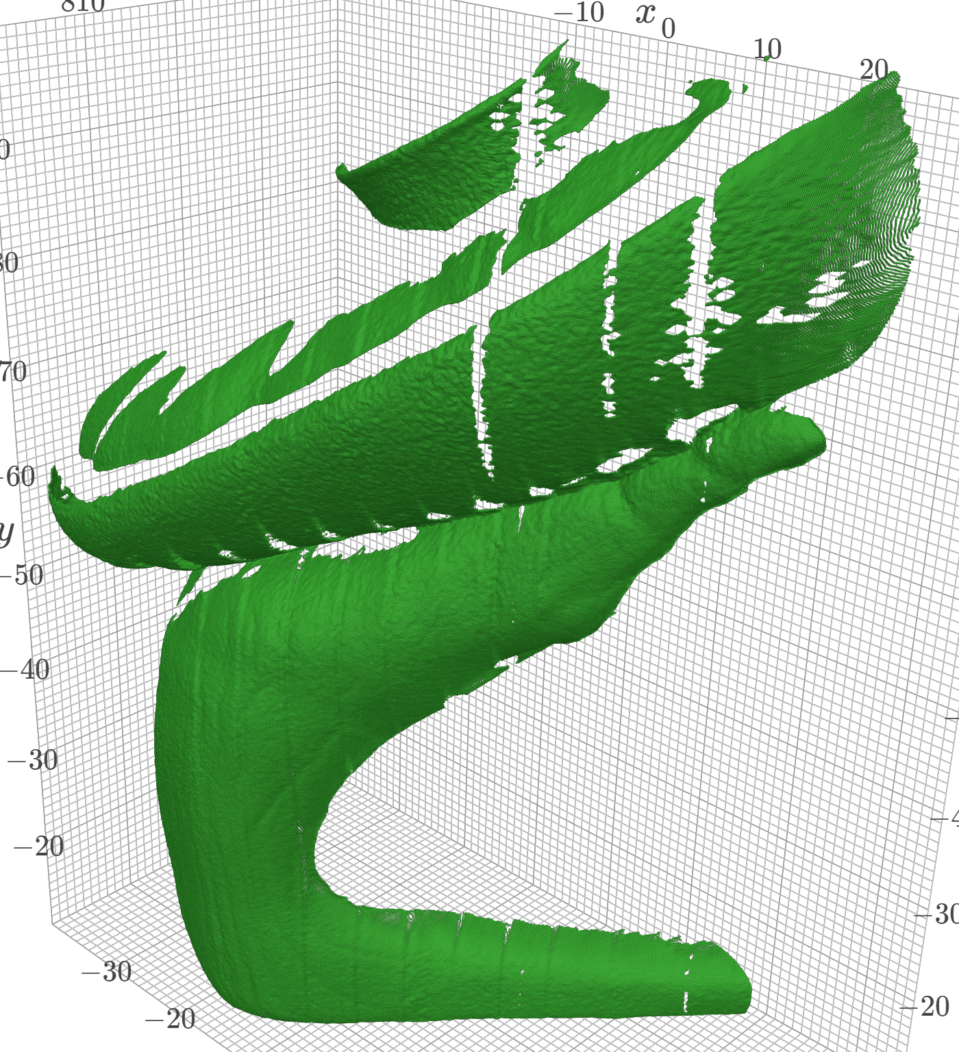
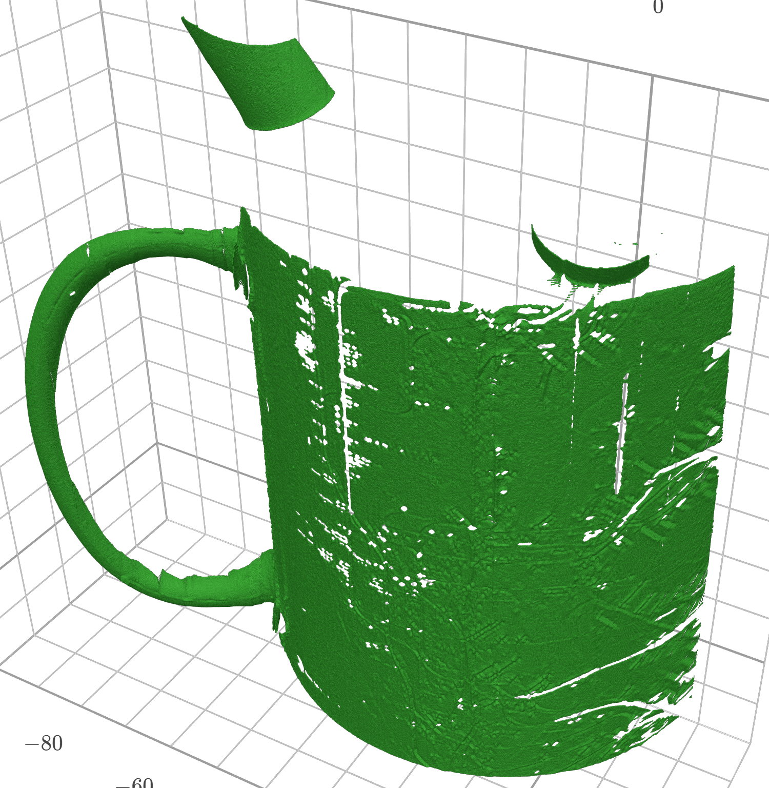
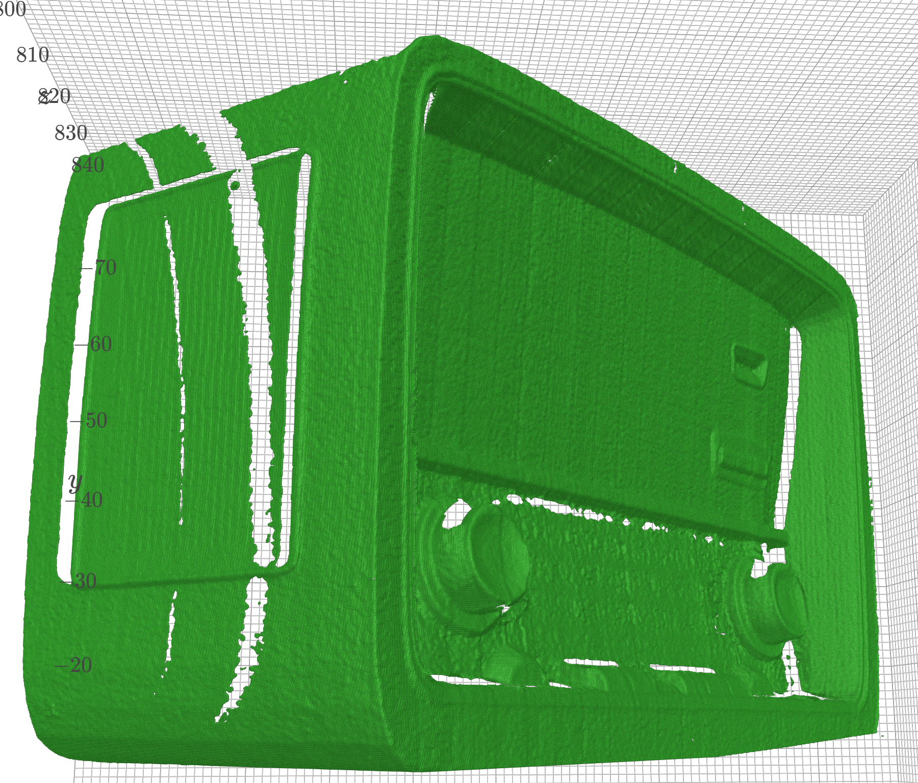
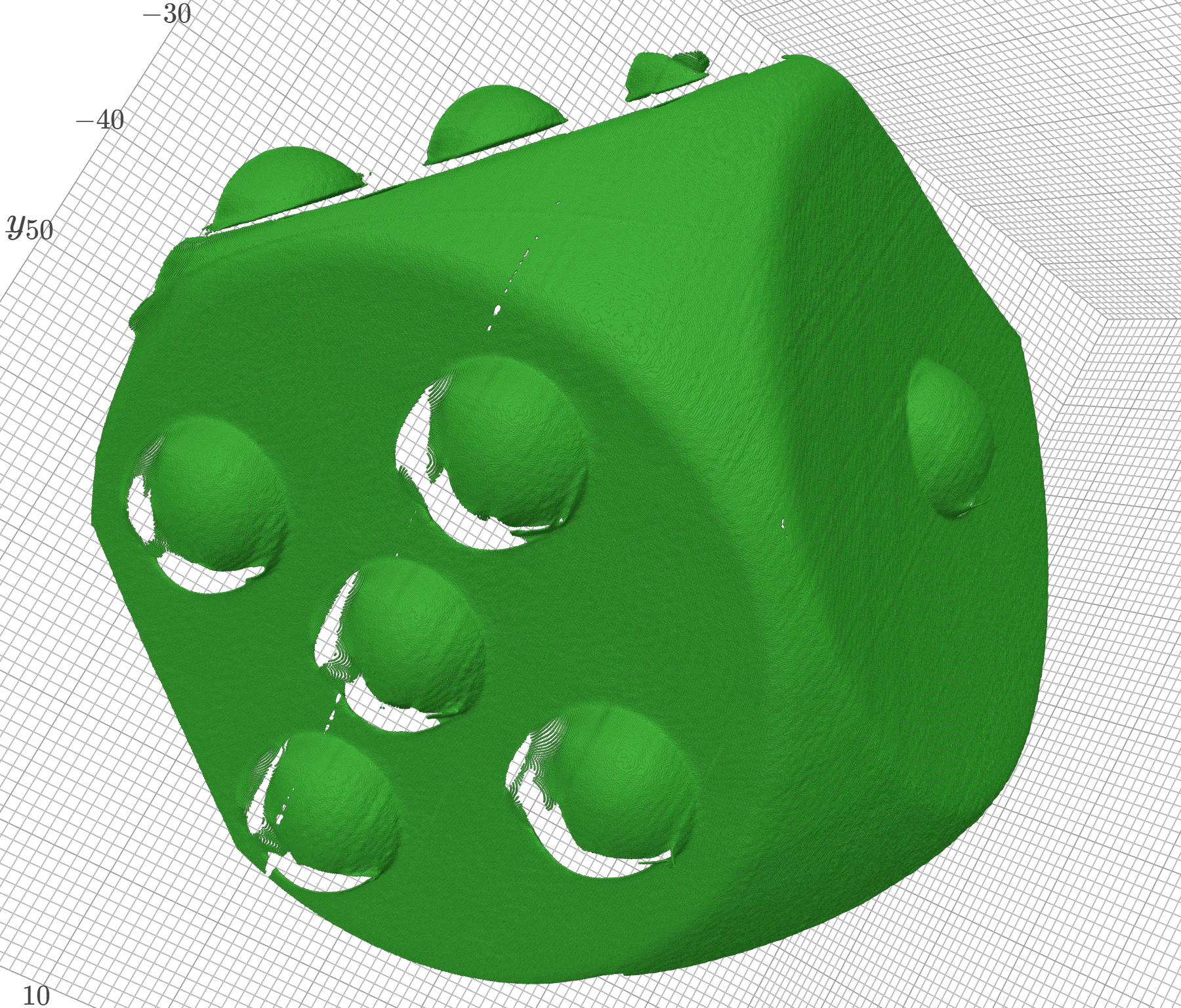
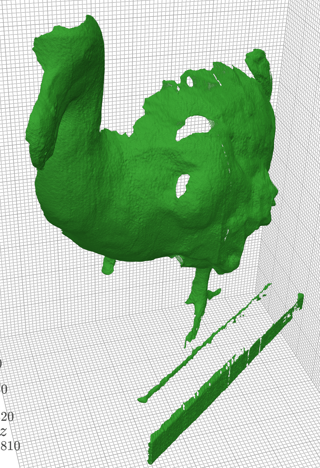
(c) Colors LookUp3D

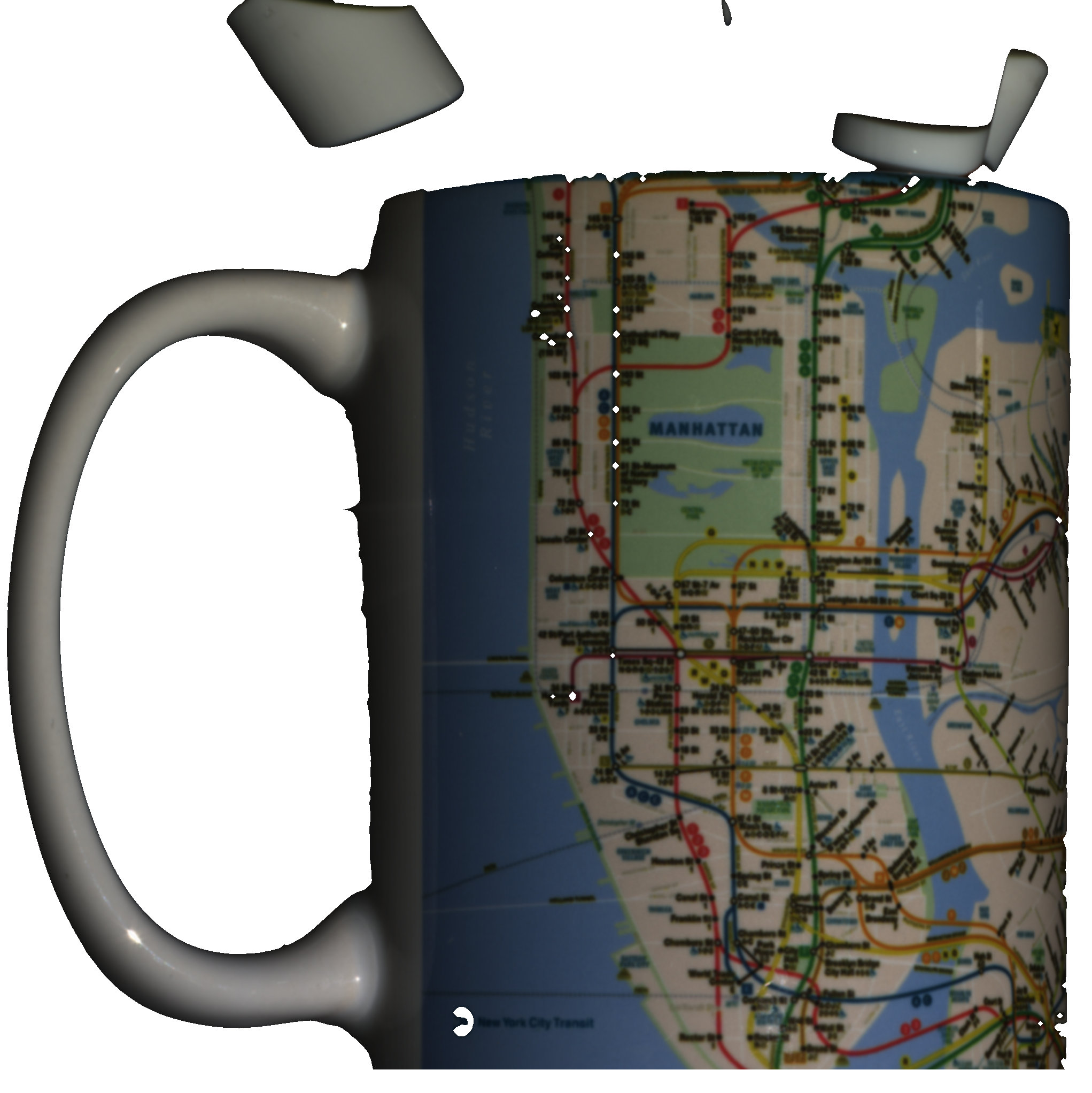
(d) White Pattern Image

Figure 9. Static Objects: here we present six different objects reconstructed using three different methods. Triangulation+ is (Koch et al., 2021), Gray LookUp3D is our method with Gray code patterns, and Colors is our method with all color patterns. These results were obtained using the digital scanner setup.

(a) $T_{0}$

(b) $T_{1}$

(c) $T_{2}$

(d) Azure Kinect

(e) RealSence

(f) Photoneo

Figure 10. Dynamic Scene 1: A cube dropping onto an inflated balloon recorded at 400 fps. We plot here three different moments: (a) the cube before hitting the balloon, (b) the cube squishing the balloon, and (c) the cube ricocheting from the balloon. We also use three commercial devices ((d) Microsoft Azure Kinect, (e) Intel Realsense 455, and (f) Photoneo) to reconstruct and qualitatively compare a similar scene of a cube bouncing off of an inflated balloon.

(a) $T_{0}$

(b) $T_{1}$

(c) $T_{2}$

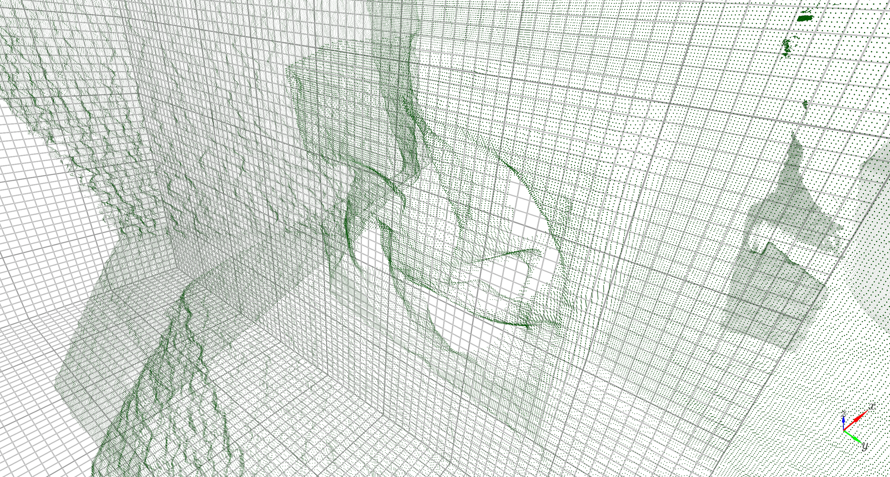
(d) Azure Kinect

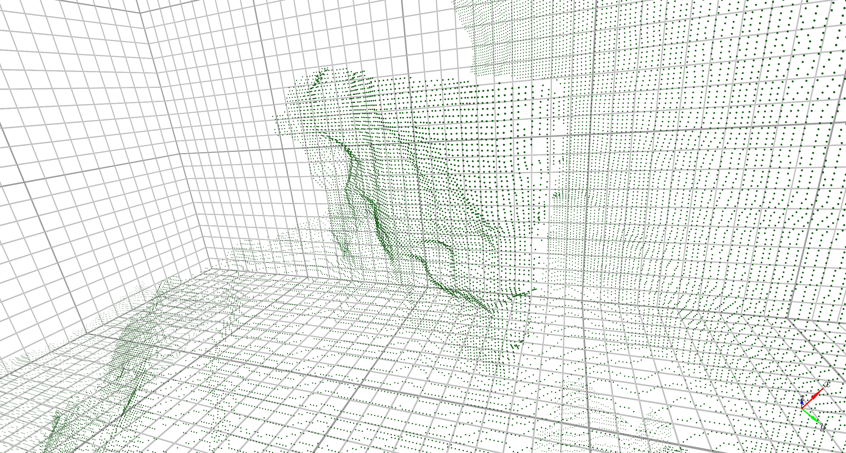
(e) RealSence

(f) Photoneo

Figure 11. Dynamic Scene 2: A fan spinning at 300 rpm. We plot three different moments (a through c) 2 frames apart when recorded at 270 fps. No temporal filtering was applied to this scene. We also use three commercial devices ((d) Microsoft Azure Kinect, (e) Intel Realsense 455, and (f) Photoneo) to reconstruct and qualitatively compare scans of the same fan rotating at the same speed.

References

- (1)
- Anon (2023a) Anon. 2023a. Kinect. https://en.wikipedia.org/w/index.php?title=Kinect&oldid=1185848427 Page Version ID: 1185848427.
- Anon (2023b) Anon. 2023b. Lissajous curve. https://en.wikipedia.org/w/index.php?title=Lissajous_curve&oldid=1187167880 Page Version ID: 1187167880.
- Anon (2023c) Anon. 2023c. PrimeSense. https://en.wikipedia.org/w/index.php?title=PrimeSense&oldid=1183798693 Page Version ID: 1183798693.
- Boyer and Kak (1987) K. L. Boyer and A. C. Kak. 1987. Color-Encoded Structured Light for Rapid Active Ranging. IEEE Transactions on Pattern Analysis and Machine Intelligence PAMI-9, 1 (Jan. 1987), 14–28. https://doi.org/10.1109/TPAMI.1987.4767869
- Carrihill and Hummel (1985) Brian Carrihill and Robert Hummel. 1985. Experiments with the intensity ratio depth sensor. Computer Vision, Graphics, and Image Processing 32, 3 (Dec. 1985), 337–358. https://doi.org/10.1016/0734-189X(85)90056-8
- Caspi et al. (1998) D. Caspi, N. Kiryati, and J. Shamir. 1998. Range imaging with adaptive color structured light. IEEE Transactions on Pattern Analysis and Machine Intelligence 20, 5 (May 1998), 470–480. https://doi.org/10.1109/34.682177
- Dobosz and Woźniak (2005) Marek Dobosz and Adam Woźniak. 2005. CMM touch trigger probes testing using a reference axis. Precision Engineering 29, 3 (July 2005), 281–289. https://doi.org/10.1016/j.precisioneng.2004.11.008
- Ferreira et al. (2013) Fernando A.M. Ferreira, Jesus De Vicente Y Oliva, and Angel M. Sanchez Perez. 2013. Evaluation of the Performance of Coordinate Measuring Machines in the Industry, Using Calibrated Artefacts. Procedia Engineering 63 (2013), 659–668. https://doi.org/10.1016/j.proeng.2013.08.232
- Furukawa and Hernández (2015) Yasutaka Furukawa and Carlos Hernández. 2015. Multi-view stereo: a tutorial. Number 9,1/2 in Foundation and trends in computer graphics and vision. Now, Boston Delft.
- Gao et al. (2015) Te Gao, Burcu Akinci, Semiha Ergan, and James Garrett. 2015. An approach to combine progressively captured point clouds for BIM update. Advanced Engineering Informatics 29, 4 (Oct. 2015), 1001–1012. https://doi.org/10.1016/j.aei.2015.08.005
- Gupta and Nayar (2012) M. Gupta and S. K. Nayar. 2012. Micro Phase Shifting. In 2012 IEEE Conference on Computer Vision and Pattern Recognition. IEEE, Providence, RI, 813–820. https://doi.org/10.1109/CVPR.2012.6247753
- Hall-Holt and Rusinkiewicz (2001) O. Hall-Holt and S. Rusinkiewicz. 2001. Stripe boundary codes for real-time structured-light range scanning of moving objects. In Proceedings Eighth IEEE International Conference on Computer Vision. ICCV 2001, Vol. 2. IEEE Comput. Soc, Vancouver, BC, Canada, 359–366. https://doi.org/10.1109/ICCV.2001.937648
- Horaud et al. (2016) Radu Horaud, Miles Hansard, Georgios Evangelidis, and Clément Ménier. 2016. An overview of depth cameras and range scanners based on time-of-flight technologies. Machine Vision and Applications 27, 7 (Oct. 2016), 1005–1020. https://doi.org/10.1007/s00138-016-0784-4
- Inokuchi et al. (1984) S. Inokuchi, K. Sata, and F. Matsuda. 1984. Range imaging system for 3-D object recognition. Proceedings of the International Conference on Pattern Recognition 1984 0, 0 (1984), 806–808.
- Je et al. (2012) Changsoo Je, Sang Wook Lee, and Rae-Hong Park. 2012. Colour-stripe permutation pattern for rapid structured-light range imaging. Optics Communications 285, 9 (May 2012), 2320–2331. https://doi.org/10.1016/j.optcom.2012.01.025
- Koch et al. (2021) Sebastian Koch, Yurii Piadyk, Markus Worchel, Marc Alexa, Cláudio Silva, Denis Zorin, and Daniele Panozzo. 2021. Hardware Design and Accurate Simulation of Structured-Light Scanning for Benchmarking of 3D Reconstruction Algorithms. In Thirty-fifth Conference on Neural Information Processing Systems Datasets and Benchmarks Track (Round 2). NeurIPS, New York. https://openreview.net/forum?id=bNL5VlTfe3p
- Lanman and Taubin (2009a) Douglas Lanman and Gabriel Taubin. 2009a. Build your own 3D scanner: 3D photography for beginners. In ACM SIGGRAPH 2009 Courses. ACM, New Orleans Louisiana, 1–94. https://doi.org/10.1145/1667239.1667247
- Lanman and Taubin (2009b) Douglas Lanman and Gabriel Taubin. 2009b. Build Your Own 3D Scanner: Optical Triangulation for Beginners. In ACM SIGGRAPH ASIA 2009 Courses (SIGGRAPH ASIA ’09). Association for Computing Machinery, New York, NY, USA, Article 2, 94 pages. https://doi.org/10.1145/1665817.1665819