Not All Language Model Features Are Linear
Abstract
Recent work has proposed the linear representation hypothesis: that language models perform computation by manipulating one-dimensional representations of concepts (“features”) in activation space. In contrast, we explore whether some language model representations may be inherently multi-dimensional. We begin by developing a rigorous definition of irreducible multi-dimensional features based on whether they can be decomposed into either independent or non-co-occurring lower-dimensional features. Motivated by these definitions, we design a scalable method that uses sparse autoencoders to automatically find multi-dimensional features in GPT-2 and Mistral 7B. These auto-discovered features include strikingly interpretable examples, e.g. circular features representing days of the week and months of the year. We identify tasks where these exact circles are used to solve computational problems involving modular arithmetic in days of the week and months of the year. Finally, we provide evidence that these circular features are indeed the fundamental unit of computation in these tasks with intervention experiments on Mistral 7B and Llama 3 8B, and we find further circular representations by breaking down the hidden states for these tasks into interpretable components.
1 Introduction
Language models trained for next-token prediction on large text corpora have demonstrated remarkable capabilities, including coding, reasoning, and in-context learning [7, 1, 3, 45]. However, the specific algorithms models learn to achieve these capabilities remain largely a mystery to researchers; we do not understand how language models write poetry. Mechanistic interpretability is a field that seeks to address this gap by reverse-engineering trained models from the ground up into variables (features) and the programs (circuits) that process these variables [37].
One mechanistic interpretability research direction has focused on understanding toy models in detail. This work has found multi-dimensional representations of inputs such as lattices [30] and circles [27, 35], and has successfully reverse-engineered the algorithms that models use to manipulate these representations. A separate direction has identified one-dimensional representations of high level concepts and quantities in large language models [15, 29, 17, 6]. These findings have led to the linear representation hypothesis: that all representations in pretrained large language models are one-dimensional lines, and that we can understand model behavior as nonlinear manipulations of these linear representations [38, 6]. In this work, we bridge the gap between these two regimes by providing evidence that language models also use multi-dimensional representations.
1.1 Contributions
-
1.
In Section 3, we generalize the one-dimensional definition of a language model feature to multi-dimensional features, provide an updated superposition hypothesis to account for these new features, and analyze the reduction in a model’s representation space implied by using multi-dimensional features. We also develop a theoretically grounded and empirically practical test for irreducible features and run this test on some sample distributions.
-
2.
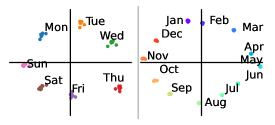
In Section 4, we present a method for finding multi-dimensional features using sparse autoencoders and identify multi-dimensional representations automatically in GPT-2 and Mistral 7B, including circular representations for the day of the week and month of the year. To the best of our knowledge, we are the first to find an emergent circular representation in a large language model.
-
3.
In Section 5, we propose two tasks, modular addition in days of the week and in months of the year, that we hypothesize will cause models to use these circular representations. We perform intervention experiments on Mistral 7B and Llama 3 8B to show that models do indeed use circular representations for these tasks. Finally, we present novel methods for decomposing LLM hidden states and reveal circles in the computed day of the week and month of the year.
2 Related Work
Linear Representations: Early word embedding methods such as GloVe and Word2vec, although only trained using co-occurrence data, contained directions in their vector spaces corresponding to semantic concepts, e.g. the well-known f(king) - f(man) + f(woman) = f(queen) [32, 40, 31]. Recent research has found similar evidence of linear representations in sequence models trained only on next token prediction, including Othello board positions [36, 26], the truth value of assertions [29], and numeric quantities such as longitude, latitude, birth year, and death year [15, 17]. These results have inspired the linear representation hypothesis [38, 11] defined above. Recent theoretical work provides evidence for this hypothesis, assuming a latent (binary) variable-based model of language [22]. Empirically, dictionary learning has shown success in breaking down a model’s feature space into a sparse over-complete basis of linear features using sparse autoencoders [6, 9]. These works assume that the number of linear features stored in superposition exceeds the model dimensionality [11].
Nonlinear Representations: There has been comparatively little research on nonlinear features. One recent paper [24] proves that a one-layer swapped order (MLP before attention) transformer can in-context-learn a nonlinear mapping function followed by a linear regression, implying that the “features” between the MLP and attention blocks are nonlinear. Another work [42] finds that a transformer trained on a hidden Markov model uses a fractal structure to represent the probability of each next token. These works analyze toy models and it is not clear if large language models will have similar nonlinear features. A separate idea [4] argues for interpreting neural networks through the polytopes they split the input space into, and identifies regions of low polytope density as “valid” regions for a potential linear representation. Finally, recent work on dictionary learning [6] has speculated about multi-dimensional feature manifolds; our work is most similar to this direction and develops the idea of feature manifolds theoretically and empirically .
Circuits: Circuits research seeks to identify and understand circuits, subsets of a model (usually represented as a directed acyclic graph) that explain specific behaviors [37]. The base units that form a circuit can be layers, neurons [37], or sparse autoencoder features [28]. The first circuits-style work looked at the InceptionV1 image model and found line features that were combined into curve detection features [37]. More recent work has examined language models, for example the indirect object identification circuit in GPT-2 [47]. Given the difficulty of designing bespoke experiments, there has been increased research in automated circuit discovery methods [28, 8, 44].
Interpretability for Arithmetic Problems: Prior work studies models trained on modular arithmetic problems and finds that models that generalize well have circular representations for and [27]. Further work shows that models use these circular representations to compute via a “clock” algorithm [35] and a separate “pizza” algorithm [49]. These papers are limited to the case of a small model trained only on modular arithmetic. Another direction has studied how large language models perform basic arithmetic, including a circuits level description of the greater-than operation in GPT-2 [16] and addition in GPT-J [43]. These works find that to perform a computation, models copy pertinent information to the token before the computed result and perform the computation in the subsequent MLP layers. Finally, recent work [14] investigates language models’ ability to increment numbers and finds linear features that fire on tokens equivalent modulo .
3 Definitions and Theory
In this section, we focus on layer transformer models that take in token input , have hidden states for layers , and output logit vectors . Given a set of inputs , we let be the set of all corresponding . This section focuses on hypotheses that describe how to decompose hidden states into sums of functions of the input (features). While this is always possible if is deterministic via the “trivial” evaluation of itself, we are interested in decomposable, interpretable hypotheses for the construction of . We write matrices in capital bold, vectors and vector valued functions in lowercase bold, and sets in capital non-bold.
3.1 Multi-Dimensional Features
Definition 1 (Feature).
We define a -dimensional feature of sparsity as a function that maps a subset of the input space of probability into a -dimensional point cloud in . We say that a feature is active on the aforementioned subset.
As an example, let (so inputs are single tokens) and consider a feature that maps integer tokens to equispaced points in . Then is a -dimensional feature that is active on integer tokens, and if integer tokens occur of the time across the input distribution, has sparsity .
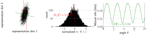
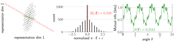
For features to be meaningful, they should be irreducible. Here, we focus on statistical reducibility: is reducible if it is composed of two statistically independent co-occurring features (in which case is “separable”) or if it is composed of two non-co-occurring features (in which case is a “mixture”). We compare this with another way to define multi-dimensional irreducibility in Appendix C.
The probability distribution over input tokens induces a -dimensional probability distribution over feature vectors — Fig. 2 shows two examples. Note that is a random vector since is a random variable; we use to denote the probability density function of .
Definition 2.
A feature is reducible into features and if there exists an affine transformation
| (1) |
for some orthonormal matrix and additive constant , such that the transformed feature probability distribution satisfies at least one of these conditions:
-
1.
is separable, i.e., factorizable as a product of its marginal distributions:
. -
2.
is a mixture of disjoint probability distributions for , and is lower-dimensional such that .
Here is the Dirac delta function. By two probability distributions being disjoint, we mean that they have disjoint support (there is no set where both have positive probability measure, or equivalently the two features and cannot be active at the same time). In Eq. 1, is the first components of the vector and is the remaining components. When is separable or a mixture, we also say that is separable or a mixture. We term a feature irreducible if it is not reducible, i.e., if no rotation and translation makes it separable or a mixture.
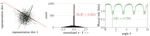
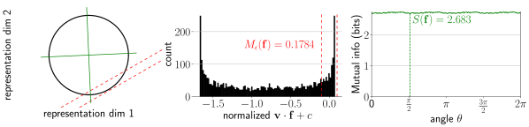
Fig. 2a shows an example of a 2D feature that is a mixture, because it can be decomposed into features and where is a 1D line distribution (marked in red) and is the remainder (a 2D cloud and a line, which can in turn be decomposed). An example of a feature that is separable is a normal distribution (since any multidimensional Gaussian can be rotated to have a diagonal covariance matrix). In natural language, a mixture might be a one hot encoding of “language of the current token”, while a separable distribution might be the “latitude” and “longitude” of location tokens.
In practice, because of noise and finite sample size, the mixture and separability definitions may not be precisely satisfied. Thus, we soften our definitions to permit degrees of reducibility:
Definition 3 (Separability Index and -Mixture Index).
Consider a feature . The separability index measures the minimal mutual information between all possible and defined in Eq. 1:
| (2) |
where denotes the mutual information. Smaller values of mean that is more separable and therefore more reducible. Note that we can solely minimize over how many components to split off as and over orthonormal matrices , since the additive offset does not affect the mutual information.
The -mixture index tests how often can be projected near zero while it is active:
| (3) |
Larger values of mean that is more of a mixture and is therefore more reducible.
We develop an optimization procedure to solve for the and in Definition 3 and apply it to synthetic feature distributions in Fig. 2a. Further details on this optimization process, more synthetic feature distributions, and more intuition about these definitions can be found in Appendix B.
3.2 Superposition
We now examine the implications of multi-dimensional features for the superposition hypothesis [11]. We first restate the original superposition hypothesis using our above definitions:
Definition 4 (-orthogonal matrices).
Two matrices and are -orthogonal if for all unit vectors and .
Hypothesis 1 (One-Dimensional Superposition Hypothesis, paraphrased from [11]).
Hidden states are the sum of many () sparse one-dimensional features and pairwise -orthogonal vectors such that . We set to zero when is outside the domain of .
We now present our new superposition hypothesis, which posits independence between irreducible multi-dimensional features instead of unknown levels of independence between one-dimensional features:
Hypothesis 2 (Our Superposition Hypothesis, changes underlined).
Hidden states are the sum of many () sparse low-dimensional irreducible features and pairwise -orthogonal matrices such that . We set to zero when is outside the domain of . Any subset of features must be mutually independent on their shared domain.
The Johnson-Lindenstrauss (JL) Lemma [23] implies that we can choose pairwise one-dimensional -orthogonal vectors to satisfy 1 for some constant , thus allowing us to build the model’s feature space with a number of one-dimensional -orthogonal features exponential in . In Appendix A, we prove a similar result for low-dimensional projections (the main idea of the proof is to combine -orthogonal vectors as guaranteed from the JL lemma):
Theorem 1.
For any , , and , it is possible to choose pairwise -orthogonal matrices where for some constant .
This exponential reduction in the number of features that are representable -orthogonally (as opposed to a multiplicative factor reduction, which is also present) suggests that models will employ higher-dimensional features only for representations that necessitate detailed multi-dimensional descriptions. Moreover, these representations will be highly compressed to fit within the smallest dimensional space possible, potentially leading to interesting encodings; for example, recent work [33] finds that maximum-margin solutions for problems like modular arithmetic consist of Fourier features. Note that the proof assumes the “worst case” scenario that all of the features are dimension , while in practice many of the features may be or low dimensional, so the effect on the capacity of a real model that represents multi-dimensional features is unlikely to be this extreme.
4 Sparse Autoencoders Find Multi-Dimensional Features
Sparse autoencoders (SAEs) deconstruct model hidden states into sparse vector sums from an over-complete basis [6, 9]. For hidden states , a one-layer SAE of size with sparsity penalty minimizes the following dictionary learning loss [6, 9]:
| (4) |
In practice, the loss on the last term is relaxed to for to make the loss differentiable. We call the columns of (vectors in ) dictionary elements.
We propose that SAEs can discover irreducible multi-dimensional features by locating point sets with a low -mixture index. For instance, if contains an irreducible two-dimensional feature (see 2), and includes just two dictionary elements spanning , both elements must have nonzero activations post-ReLU to perfectly reconstruct (otherwise is a mixture). Thus the Jaccard similarity of the sets of tokens that these two dictionary elements fire on is likely to be high. On the other hand, if contains more than two dictionary elements that span , then the Jaccard similarity may be lower. However, since there are now many dictionary elements with a high projection in the two dimensional feature space, the cosine similarity of the dictionary elements is likely to be high.
Thus for a two dimensional irreducible feature , we expect there to be groups of dictionary elements with either high cosine or Jaccard similarity corresponding to . We expect this observation to be true for higher dimensional irreducible features as well. Note that some clusters may correspond to separable features , as this technique only finds features that are not mixtures. This suggests a natural approach to using sparse autoencoders to search for irreducible multi-dimensional features:
1. Cluster dictionary elements by their pairwise cosine similarity or Jaccard similarity.
2. For each cluster, run the SAEs on all and ablate all dictionary elements not in the cluster. This will give the reconstruction of each restricted to the cluster found in step (if no cluster dictionary elements are non-zero for a given point, we ignore the point).
3. Examine the resulting reconstructed activation vectors for irreducible multi-dimensional features, especially ensuring that the reconstruction is not separable. This step can be done manually by visually inspecting the PCA projections for known irreducible multi-dimensional structures (e.g. circles, see Fig. 2) or automatically by passing the PCA projections to the tests for Definition 3.
| Model | Weekdays | Months |
|---|---|---|
| Llama 3 8B | 29 / 49 | 143 / 144 |
| Mistral 7B | 31 / 49 | 125 / 144 |
| GPT-2 | 8 / 49 | 10 / 144 |
This method succeeds on toy datasets of synthetic irreducible multi-dimensional features; see Appendix D.111Code for reproducing experiments: https://github.com/JoshEngels/MultiDimensionalFeatures We apply this method to language models using GPT-2 [41] SAEs trained by Bloom for every layer [5] and Mistral 7B [21] SAEs that we train on layers 8, 16, and 24 (training details in Appendix E). Clustering details are in Appendix F, including comments on scalability.
5 Circular Representations in Large Language Models
In this section, we seek tasks in which models use the multi-dimensional features we discovered in Section 4, thereby providing evidence that these representations are indeed the fundamental unit of computation for some problems. Inspired by prior work studying circular representations in modular arithmetic [27], we define two prompts that represent “natural” modular arithmetic tasks:
Weekdays task: “Let’s do some day of the week math. Two days from Monday is”
Months task: “Let’s do some calendar math. Four months from January is”
For Weekdays, we range over the days of the week and durations between and days to get prompts. For Months, we range over the months of the year and durations between and months to get prompts. Mistral 7B and Llama 3 8B [2] achieve reasonable performance on the Weekdays task and excellent performance on the Months task (measured by comparing the highest logit valid token against the ground truth answer), as summarized in Table 1. Interestingly, although these problems are equivalent to modular arithmetic problems for , both models get trivial accuracy on plain modular addition prompts, e.g. “”. Finally, although GPT-2 has circular representations, it gets trivial accuracy on Weekdays and Months.
To simplify discussion, let be the day of the week or month of the year token (e.g. “Monday” or “April”), be the duration token (e.g. “four” or “eleven”), and be the target ground truth token the model should predict, such that (abusing notation) we have . Let the prompts of the task be parameterized by , such that the th prompt asks about , , and .
5.1 Intervening on Circular Day and Month Representations
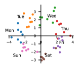
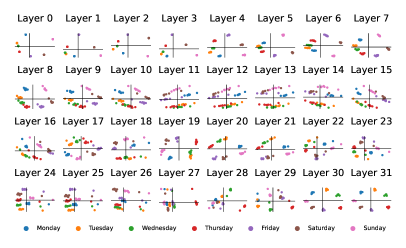
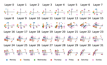
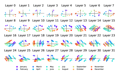
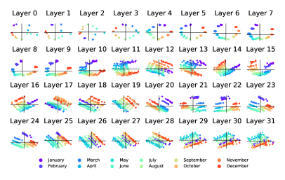
We first confirm that Llama 3 8B and Mistral 7B have circular representations of by examining the PCA of hidden states across prompts at various layers on the token. We plot two of these in Fig. 3 and show all layers in Fig. 14 in the appendix. These plots show circular representations as the highest varying two components in the model’s representation of at many layers.
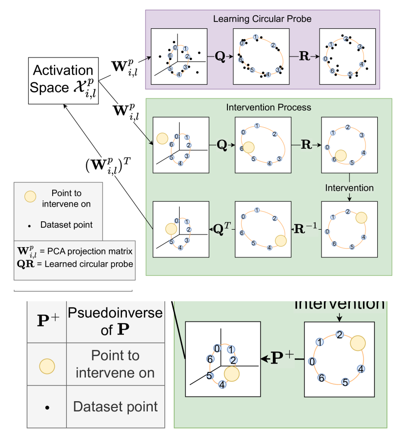
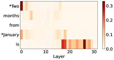
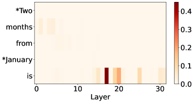
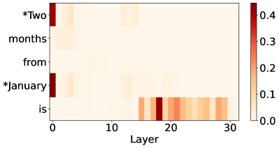
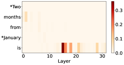
We now experiment with intervening on these circular representations. We base our experiments on the common interpretability technique of activation patching, which replaces activations from a “dirty” run of the model with the corresponding activations from a “clean” run [48]. Activation patching empirically tests whether a specific model component, position, and/or representation has a causal influence on the model’s output. We employ a custom subspace patching method to allow testing for whether a specific circular subspace of a hidden state is sufficient to causally explain model output. Specifically, our patching technique relies on the following steps (visualized in Fig. 5):
1. Find a subspace with a circle to intervene on: Using a PCA reduced activation subspace to avoid overfitting, we train a “circular probe” to identify representations which exhibit strong circular patterns. More formally, let be the hidden state at layer token position for prompt . Let be the matrix consisting of the top principal component directions of . In our experiments, we set . We learn a linear probe from to a unit circle in . In other words, if for Weekdays and for Months, is defined as follows:
| (5) |
2. Intervene on the subspace: Say our initial prompt had and we are intervening with . In this step, we replace the model’s projection on the subspace , which will be close to ), with the “clean” point . Note that we do not use the hidden state from the “clean” run, only the “clean” label . In practice, other subspaces of may be used by the model in alternate pathways to compute the answer. To avoid this affecting the intervention, we average out all subspaces not in the intervened subspace. Letting be the average of across all prompts indexed by and be the pseudoinverse of , we intervene via the formula
| (6) |
We run our patching on all Weekday problems and Month problems and use as “clean” runs the or other possible values for , resulting in a total of patching experiments for Weekdays and patching experiments for Months. We also run baselines where we
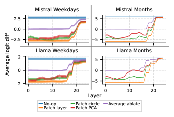
(1) replace the entire subspace corresponding to the first PCA dimensions with the corresponding subspace from the clean run, (2) replace the entire layer with the corresponding layer from the clean run, and (3) replace the entire layer with the average across the task. The metric we use is average logit difference across all patching experiments between the original correct token () and the target token (). See Fig. 5 for these interventions on all layers of Mistral 7B and Llama 3 8B on Weekdays and Months.
The main takeaway from Fig. 5 is that circular subspaces are causally implicated in computing , especially for Weekdays. Across all models and tasks, early layer interventions on the circular subspace have almost the same intervention effect as patching the entire layer, and are sometimes even better than patching the top PCA dimensions from the clean problem. Note that patching experiments in Appendix I show is copied to the final token on layers to , which is why interventions drop off there.
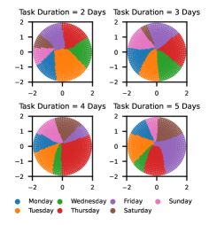
To investigate exactly how models use the circular subspace, we perform off distribution interventions. We modify Eq. 6 so that instead of intervening on the circumference , we sweep over a grid of positions within the circle:
| (7) |
We intervene with and record the highest logit after the forward pass. Fig. 6 displays these results on Mistral layer for . They imply that Mistral treats the circle as a multi-dimensional representation with encoded in the angle.
5.2 Decomposing Hidden States
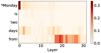
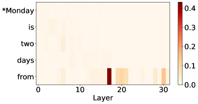
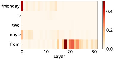
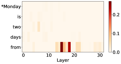
To isolate the rough circuit for Weekdays and Months, we perform layer-wise activation patching on random pairs of prompts. The results, displayed in Appendix I, show that the circuit to compute consists of MLPs on top of the and tokens, a copy to the token before , and further MLPs there (roughly similar to prior work studying arithmetic circuits [43]). Moreover, fine-grained patching in Appendix I shows that there are just a few responsible attention heads for the writes to the token before . However, patching alone cannot tell use how or where is represented.
We now introduce a new technique for empirically explaining hidden representations in algorithmic problems: explanation via regression (EVR). Given a set of tokens with a corresponding set of hidden states , we explain the variance in by adding together hand-chosen functions of . This gives us an explanation of what the transformation computes. For a given choice of explanation functions , the value of a linear regression from to gives a measure of the explained variance in . But what functions should we choose?
We build a list of iteratively and greedily. At each iteration, we perform a linear regression with the current list , visualize and interpret the residual prediction errors, and build a new function representing these errors to add to the list. Once most variance is explained, we can conclude that constitutes the entirety of what is represented in the hidden states. This information tells us what can and cannot be extracted via a linear probe, without having to train any probes. Furthermore, if we treat each as a feature (see Definition 1), then the linear regression coefficients tell us which directions in these features are represented in, connecting back to 2.
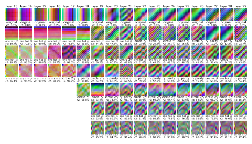
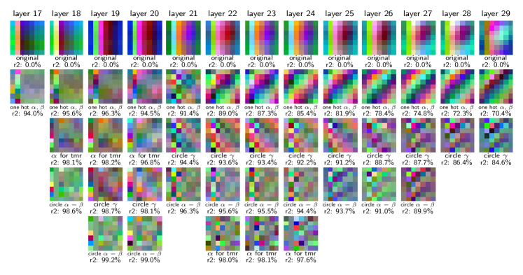
We apply EVR to Months and Weekdays. Since consists of modular addition problems with two inputs and , we can visualize the errors as we iteratively construct by making a heatmap with and on the two axes, where the color shows what kind of error is made. More specifically, we take the top 3 PCA components of the error distribution and assign them to the colors red, green, and blue. We call the resulting heatmap a residual RGB plot. Errors that depend primarily on , , or show up as horizontal, vertical, or diagonal stripes on the residual RGB plot.
In Fig. 8, we perform EVR on the layer 17-29 hidden states of Mistral 7B on the Weekdays task; additional deconstructions are in Appendix I. We find that a circle in develops and grows in explanatory power; we plot the layer residuals after explaining with one hot functions in and (i.e. ) in Fig. 7 to show this incredibly clear circle in . This suggests that the models may be generating by using a trigonometry based algorithm like the “clock” [35] or “pizza” [49] algorithm in late MLP layers.
6 Discussion
Our work proposes a significant refinement to the simple one-dimensional linear representation hypothesis. While previous work has convincingly shown the existence of one-dimensional features, we find evidence for multi-dimensional representations that are non-separable and irreducible, requiring us to generalize the notion of a feature to higher dimensions. Fortunately, we find that existing feature extraction methodologies like sparse autoencoders can readily be applied to discover multi-dimensional representations. Although multi-dimensional representations may be more complicated, we believe that uncovering the true (perhaps multi-dimensional) nature of model representations is necessary for discovering the underlying algorithms that use these representations. Ultimately, we aim to turn complex circuits in future more-capable models into formally verifiable programs [46, 10], which requires the ground truth “variables” of language models; we believe this work takes an important step towards discovering these variables. Finally, we do not anticipate adverse impacts of our work, as it focuses only on deepening our understanding of language model representations.
Limitations:
It is unclear why we did not find more interpretable multi-dimensional features: are there truly not that many, or is our clustering technique failing to find them? Our definition for an irreducible feature (Definition 2) also had to be relaxed to hold in practice (Definition 3). Thus, although this work provides preliminary evidence for the multi-dimensional superposition hypothesis (2), it is still unclear if this theory provides the best description for the representations models use. We also did not find a small subset of MLP neurons implementing the “clock” algorithm, leaving as an open question to what extent models use multi-dimensional representations for algorithmic tasks. Finally, we only ran experiments on models up to size 8B; however, recent work [20] implies representations may become universal with growing model size.
Acknowledgments and Disclosure of Funding
We thank (in alphabetical order) Dowon Baek, Kaivu Hariharan, Vedang Lad, Ziming Liu, and Tony Wang for helpful discussions and suggestions. This work is supported by Erik Otto, Jaan Tallinn, the Rothberg Family Fund for Cognitive Science, the NSF Graduate Research Fellowship (Grant No. 2141064), and IAIFI through NSF grant PHY-2019786.
References
- [1] Josh Achiam, Steven Adler, Sandhini Agarwal, Lama Ahmad, Ilge Akkaya, Florencia Leoni Aleman, Diogo Almeida, Janko Altenschmidt, Sam Altman, Shyamal Anadkat, et al. Gpt-4 technical report. arXiv preprint arXiv:2303.08774, 2023.
- [2] AI@Meta. Llama 3 model card, 2024.
- [3] Anthropic. The claude 3 model family: Opus, sonnet, haiku. Technical report, Anthropic, 2024.
- [4] Sid Black, Lee Sharkey, Leo Grinsztajn, Eric Winsor, Dan Braun, Jacob Merizian, Kip Parker, Carlos Ramón Guevara, Beren Millidge, Gabriel Alfour, et al. Interpreting neural networks through the polytope lens. arXiv preprint arXiv:2211.12312, 2022.
- [5] Joseph Bloom. Open source sparse autoencoders for all residual stream layers of gpt2 small. https://www.alignmentforum.org/posts/f9EgfLSurAiqRJySD/open-source-sparse-autoencoders-for-all-residual-stream, 2024.
- [6] Trenton Bricken, Adly Templeton, Joshua Batson, Brian Chen, Adam Jermyn, Tom Conerly, Nick Turner, Cem Anil, Carson Denison, Amanda Askell, Robert Lasenby, Yifan Wu, Shauna Kravec, Nicholas Schiefer, Tim Maxwell, Nicholas Joseph, Zac Hatfield-Dodds, Alex Tamkin, Karina Nguyen, Brayden McLean, Josiah E Burke, Tristan Hume, Shan Carter, Tom Henighan, and Christopher Olah. Towards monosemanticity: Decomposing language models with dictionary learning. Transformer Circuits Thread, 2023. https://transformer-circuits.pub/2023/monosemantic-features/index.html.
- [7] Sébastien Bubeck, Varun Chandrasekaran, Ronen Eldan, Johannes Gehrke, Eric Horvitz, Ece Kamar, Peter Lee, Yin Tat Lee, Yuanzhi Li, Scott Lundberg, et al. Sparks of artificial general intelligence: Early experiments with gpt-4. arXiv preprint arXiv:2303.12712, 2023.
- [8] Arthur Conmy, Augustine Mavor-Parker, Aengus Lynch, Stefan Heimersheim, and Adrià Garriga-Alonso. Towards automated circuit discovery for mechanistic interpretability. Advances in Neural Information Processing Systems, 36:16318–16352, 2023.
- [9] Hoagy Cunningham, Aidan Ewart, Logan Riggs, Robert Huben, and Lee Sharkey. Sparse autoencoders find highly interpretable features in language models. arXiv preprint arXiv:2309.08600, 2023.
- [10] David Dalrymple, Joar Skalse, Yoshua Bengio, Stuart Russell, Max Tegmark, Sanjit Seshia, Steve Omohundro, Christian Szegedy, Ben Goldhaber, Nora Ammann, et al. Towards guaranteed safe ai: A framework for ensuring robust and reliable ai systems. arXiv preprint arXiv:2405.06624, 2024.
- [11] Nelson Elhage, Tristan Hume, Catherine Olsson, Nicholas Schiefer, Tom Henighan, Shauna Kravec, Zac Hatfield-Dodds, Robert Lasenby, Dawn Drain, Carol Chen, Roger Grosse, Sam McCandlish, Jared Kaplan, Dario Amodei, Martin Wattenberg, and Christopher Olah. Toy models of superposition. Transformer Circuits Thread, 2022. https://transformer-circuits.pub/2022/toy_model/index.html.
- [12] Leo Gao, Stella Biderman, Sid Black, Laurence Golding, Travis Hoppe, Charles Foster, Jason Phang, Horace He, Anish Thite, Noa Nabeshima, et al. The pile: An 800gb dataset of diverse text for language modeling. arXiv preprint arXiv:2101.00027, 2020.
- [13] Semyon Aranovich Gershgorin. über die abgrenzung der eigenwerte einer matrix. Izvestiya Rossiĭskoi akademii nauk. Seriya matematicheskaya, (6):749–754, 1931.
- [14] Rhys Gould, Euan Ong, George Ogden, and Arthur Conmy. Successor heads: Recurring, interpretable attention heads in the wild. arXiv preprint arXiv:2312.09230, 2023.
- [15] Wes Gurnee and Max Tegmark. Language models represent space and time. arXiv preprint arXiv:2310.02207, 2023.
- [16] Michael Hanna, Ollie Liu, and Alexandre Variengien. How does gpt-2 compute greater-than?: Interpreting mathematical abilities in a pre-trained language model. Advances in Neural Information Processing Systems, 36, 2024.
- [17] Benjamin Heinzerling and Kentaro Inui. Monotonic representation of numeric properties in language models. arXiv preprint arXiv:2403.10381, 2024.
- [18] Nicholas J. Higham. Singular value inequalities. https://nhigham.com/2021/05/04/singular-value-inequalities/, May 2021.
- [19] Bill Johnson (https://mathoverflow.net/users/2554/bill johnson). Almost orthogonal vectors. MathOverflow. URL:https://mathoverflow.net/q/24873 (version: 2010-05-16).
- [20] Minyoung Huh, Brian Cheung, Tongzhou Wang, and Phillip Isola. The platonic representation hypothesis. arXiv preprint arXiv:2405.07987, 2024.
- [21] Albert Q Jiang, Alexandre Sablayrolles, Arthur Mensch, Chris Bamford, Devendra Singh Chaplot, Diego de las Casas, Florian Bressand, Gianna Lengyel, Guillaume Lample, Lucile Saulnier, et al. Mistral 7b. arXiv preprint arXiv:2310.06825, 2023.
- [22] Yibo Jiang, Goutham Rajendran, Pradeep Ravikumar, Bryon Aragam, and Victor Veitch. On the origins of linear representations in large language models. arXiv preprint arXiv:2403.03867, 2024.
- [23] William B. Johnson and Joram Lindenstrauss. Extensions of lipschitz mappings into a hilbert space. In Conference in modern analysis and probability (New Haven, Conn., 1982), volume 26 of Contemporary Mathematics, pages 189–206. American Mathematical Society, Providence, RI, 1984.
- [24] Juno Kim and Taiji Suzuki. Transformers learn nonlinear features in context: Nonconvex mean-field dynamics on the attention landscape. arXiv preprint arXiv:2402.01258, 2024.
- [25] Silvio Lattanzi, Thomas Lavastida, Kefu Lu, and Benjamin Moseley. A framework for parallelizing hierarchical clustering methods. In Machine Learning and Knowledge Discovery in Databases: European Conference, ECML PKDD 2019, Würzburg, Germany, September 16–20, 2019, Proceedings, Part I, pages 73–89. Springer, 2020.
- [26] Kenneth Li, Aspen K Hopkins, David Bau, Fernanda Viégas, Hanspeter Pfister, and Martin Wattenberg. Emergent world representations: Exploring a sequence model trained on a synthetic task. arXiv preprint arXiv:2210.13382, 2022.
- [27] Ziming Liu, Ouail Kitouni, Niklas S Nolte, Eric Michaud, Max Tegmark, and Mike Williams. Towards understanding grokking: An effective theory of representation learning. Advances in Neural Information Processing Systems, 35:34651–34663, 2022.
- [28] Samuel Marks, Can Rager, Eric J Michaud, Yonatan Belinkov, David Bau, and Aaron Mueller. Sparse feature circuits: Discovering and editing interpretable causal graphs in language models. arXiv preprint arXiv:2403.19647, 2024.
- [29] Samuel Marks and Max Tegmark. The geometry of truth: Emergent linear structure in large language model representations of true/false datasets. arXiv preprint arXiv:2310.06824, 2023.
- [30] Eric J Michaud, Isaac Liao, Vedang Lad, Ziming Liu, Anish Mudide, Chloe Loughridge, Zifan Carl Guo, Tara Rezaei Kheirkhah, Mateja Vukelić, and Max Tegmark. Opening the ai black box: program synthesis via mechanistic interpretability. arXiv preprint arXiv:2402.05110, 2024.
- [31] Tomas Mikolov, Ilya Sutskever, Kai Chen, Greg S Corrado, and Jeff Dean. Distributed representations of words and phrases and their compositionality. Advances in neural information processing systems, 26, 2013.
- [32] Tomáš Mikolov, Wen-tau Yih, and Geoffrey Zweig. Linguistic regularities in continuous space word representations. In Proceedings of the 2013 conference of the north american chapter of the association for computational linguistics: Human language technologies, pages 746–751, 2013.
- [33] Depen Morwani, Benjamin L Edelman, Costin-Andrei Oncescu, Rosie Zhao, and Sham Kakade. Feature emergence via margin maximization: case studies in algebraic tasks. arXiv preprint arXiv:2311.07568, 2023.
- [34] Neel Nanda and Joseph Bloom. Transformerlens. https://github.com/TransformerLensOrg/TransformerLens, 2022.
- [35] Neel Nanda, Lawrence Chan, Tom Lieberum, Jess Smith, and Jacob Steinhardt. Progress measures for grokking via mechanistic interpretability. arXiv preprint arXiv:2301.05217, 2023.
- [36] Neel Nanda, Andrew Lee, and Martin Wattenberg. Emergent linear representations in world models of self-supervised sequence models. arXiv preprint arXiv:2309.00941, 2023.
- [37] Chris Olah, Nick Cammarata, Ludwig Schubert, Gabriel Goh, Michael Petrov, and Shan Carter. Zoom in: An introduction to circuits. Distill, 2020. https://distill.pub/2020/circuits/zoom-in.
- [38] Kiho Park, Yo Joong Choe, and Victor Veitch. The linear representation hypothesis and the geometry of large language models. arXiv preprint arXiv:2311.03658, 2023.
- [39] Baolin Peng, Chunyuan Li, Pengcheng He, Michel Galley, and Jianfeng Gao. Instruction tuning with gpt-4. arXiv preprint arXiv:2304.03277, 2023.
- [40] Jeffrey Pennington, Richard Socher, and Christopher D Manning. Glove: Global vectors for word representation. In Proceedings of the 2014 conference on empirical methods in natural language processing (EMNLP), pages 1532–1543, 2014.
- [41] Alec Radford, Jeffrey Wu, Rewon Child, David Luan, Dario Amodei, Ilya Sutskever, et al. Language models are unsupervised multitask learners. OpenAI blog, 2019.
- [42] Adam Shai, Paul Riechers, Lucas Teixeira, Alexander Oldenziel, and Sarah Marzen. Transformers represent belief state geometry in their residual stream. https://www.alignmentforum.org/posts/gTZ2SxesbHckJ3CkF/transformers-represent-belief-state-geometry-in-their, 2024.
- [43] Alessandro Stolfo, Yonatan Belinkov, and Mrinmaya Sachan. A mechanistic interpretation of arithmetic reasoning in language models using causal mediation analysis. In Proceedings of the 2023 Conference on Empirical Methods in Natural Language Processing, pages 7035–7052, 2023.
- [44] Aaquib Syed, Can Rager, and Arthur Conmy. Attribution patching outperforms automated circuit discovery. arXiv preprint arXiv:2310.10348, 2023.
- [45] Gemini Team, Rohan Anil, Sebastian Borgeaud, Yonghui Wu, Jean-Baptiste Alayrac, Jiahui Yu, Radu Soricut, Johan Schalkwyk, Andrew M Dai, Anja Hauth, et al. Gemini: a family of highly capable multimodal models. arXiv preprint arXiv:2312.11805, 2023.
- [46] Max Tegmark and Steve Omohundro. Provably safe systems: the only path to controllable agi. arXiv preprint arXiv:2309.01933, 2023.
- [47] Kevin Wang, Alexandre Variengien, Arthur Conmy, Buck Shlegeris, and Jacob Steinhardt. Interpretability in the wild: a circuit for indirect object identification in gpt-2 small. arXiv preprint arXiv:2211.00593, 2022.
- [48] Fred Zhang and Neel Nanda. Towards best practices of activation patching in language models: Metrics and methods. arXiv preprint arXiv:2309.16042, 2023.
- [49] Ziqian Zhong, Ziming Liu, Max Tegmark, and Jacob Andreas. The clock and the pizza: Two stories in mechanistic explanation of neural networks. Advances in Neural Information Processing Systems, 36, 2024.
Appendix A Proofs
We will first prove a lemma that will help us prove 1.
Lemma 1.
Pick pairwise -orthogonal unit vectors in . Let be a unit norm vector that is a linear combination of unit norm vectors with coefficients . We can write and , so that we have with . Then,
Proof.
We will first bound the norm of . If is the minimum singular value of , then we have via standard singular value inequalities [18]
Thus we now lower bound . The singular values are the square roots of the eigenvalues of the matrix , so we now examine . Since all elements of are unit vectors, the diagonal of is all ones. The off diagonal elements are dot products of pairs of -orthogonal vectors, and so are within the range . Then by the Gershgorin circle theorem [13], all eigenvalues of are in the range
In particular, , and thus . Plugging into our upper bound for , we have that . Finally, the largest for a point on an -hypersphere of radius is when all dimensions are equal and such a point has magnitude , so
∎
See 1
Proof.
By the JL lemma [23, 19], for any and , we can choose -orthogonal unit vectors in indexed as , for some constant . Let where each element in the brackets is a column. Then by construction all are matrices composed of unique -orthogonal vectors and there are matrices .
Now, consider two of these matrices and , ; we will prove that they are -orthogonal for some function . Let be a vector in the colspace of and be a vector in the colspace of , such that and are unit vectors. To prove -orthogonality, we must bound the absolute dot product between and :
| Triangle Inequality | ||||
| All are orthogonal | ||||
| Factoring the product | ||||
| By Lemma 1 | ||||
| by assumption | ||||
Thus and are -orthogonal for , and so it is possible to choose pairwise -orthogonal projection matrices. Remapping the variable with , we find that it is possible to choose pairwise -orthogonal projection matrices. Because is at most with , we can further simplify the exponent and find that it is possible to choose pairwise -orthogonal projection matrices. Absorbing the into the constant finishes the proof. ∎
Appendix B More on Reducibility
B.1 Additional Intuition for Definitions
Here, we present some extra intuition and high level ideas for understanding our definitions and the motivation behind them. Roughly, we intend for our definitions in the main text to identify representations in the model that describe an object or concept in a way that fundamentally takes multiple dimensions. We operationalize this as finding a subspace of representations that 1. has basis vectors that “always co-occur” no matter the orientation 2. is not made up of combinations of independent lower-dimensional features.
1. The first condition is met by the mixture part of our definition. The feature in question should be part of an irreducible manifold, and so should “fill” a plane or hyperplane. There shouldn’t be any part of the plane where the probability distribution of the feature is concentrated, because this region is then likely part of a lower dimensional feature. The idea of this part of the definition is to capture multi-dimensional objects; if the entire multi-dimensional space is truly being used to represent a high-dimensional object, then the representations for the object should be “spread out” entirely through the space.
2. The second condition is met by the separability part of our definition. This part of the definition is intended to rule out features that co-occur frequently but are fundamentally not describing the same object or concept. For example, latitude and longitude are not a mixture in that they frequently co-occur, but we do not think it is necessarily correct to say they are part of the same multi-dimensional feature because they are independent.
B.2 Empirical Irreducible Feature Test Details
Our tests for reducibility require the computation of two quantities for the separability index and for the -mixture index. We describe how we compute each index in the following two subsections.
B.2.1 Separability Index
We define the separability index in Equation 2 as
where the min is over rotations used to split into and . In two dimensions, the rotation is defined by a single angle, so we can iterate over a grid of 1000 angles and estimate the mutual information between and for each angle. We first normalize by subtracting off the mean and then dividing by the root mean squared norm of (and multiplying by since the toy datasets are in two dimensions). To estimate the mutual information, we first clip the data to a 6 by 6 square centered on the origin. We then bin the points into a 40 by 40 grid, to produce a discrete distribution . After computing the marginals and by summing the distribution over each axis, we obtain the mutual information via the formula
| (8) |
B.2.2 -Mixture Index
We define the -mixture index in Equation 3 as
The challenge with computing is to compute the maximum. We opted to maximize via gradient descent; and we guaranteed differentiability by softening the inequality with a sigmoid,
| (9) |
where is a temperature, which we linearly decay from to throughout training. We optimize for and using this loss using full batch gradient descent over 10000 steps with learning rate . With the solution , the final value of is then our estimate of .
We also run the irreducibility tests on additional synthetic feature distributions in Fig. 9a and Fig. 9b.
Appendix C Alternative Definitions
In this section, we present an alternative definition of a reducible feature that we considered during our work. This chiefly deals with multi-dimensional features from the angle of computational reducibility as opposed to statistical reducibility. In other words, this definition considers whether representations of features on a specific set of tasks can be split up without changing the accuracy of the task. This captures an interesting (and important) aspect of feature reducibility, but because it requires a specific set of prompts (as opposed to allowing unsupervised discovery) we chose not to use it as our main definition.
Our alternative definitions consider representation spaces that are possibly multi-dimensional, and defines these spaces through whether they can completely explain a function on the output logits. We consider a group theoretic approach to irreducible representations, via whether computation involving multiple group elements can be decomposed.
C.1 Alternative Definition: Interventions and Representation Spaces
Assume that we restrict the input set of prompts to some subset of prompts and that we have some evaluation function that maps from the output logit distribution of to a real number. For example, for the Weekdays problems, is the set of prompts and could be the over the days of week logits. Abusing notation, we let also be the function from the layer we are intervening on; this is always clear from context. Then we can define a representation space of as a subspace in which interventions always work:
Definition 5 (Representation Space).
Given a prompt set , a rank- dimensional representation space of intermediate value is a rank projection matrix such that for all , .
Note that it immediately follows that the rank dimensional matrix is trivially a rank representation space for all prompt sets .
Definition 6 (Minimality).
A representation space of rank is minimal if there does not exist a lower rank representation space.
A minimal representation with rank > 1 is a multi-dimensional representation.
Definition 7 (Alternative Reducibility).
A representation space of rank is reducible if there are orthonormal representation spaces and (such that , ) where
for all .
Suppose , and define the multiplication of two elements in a finite group of order . Then if we interpret the embedding vectors as the group representations, our definition of reducibility implies to the standard group-theoretical definition of irreducibility –– specifically, reducibility into a tensor product representation.
Appendix D Toy Case of Training SAEs on Circles
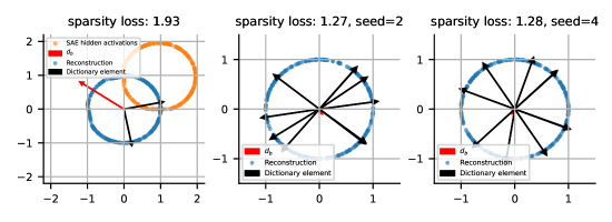
To explore how SAEs behave when reconstructing irreducible features of dimension , we perform experiments with the following toy setup. Inspired by the circular representations of integers that networks learn when trained on modular addition [35, 27], we create synthetic datasets of activations containing multiple features which are each 2d irreducible circles.
First however, consider activations for a single circle – points uniformly distributed on the unit circle in . We train SAEs on this data with encoder and decoder . We train SAEs with and with the Adam optimizer and a learning rate of , sparsity penalty , for 20,000 steps, and a warmup of 1000 steps. In Fig. 10 we show the dictionary elements of these SAEs. When , the network must use both SAE features on each input point, and uses to shift the reconstructed circle so it is centered at the origin. When , and the features spread out across the circle having close neighbors, with only a subset being active on any one input.
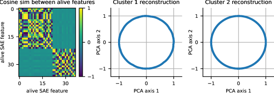
We now consider synthetic activations with multiple circular features. Our data consists of points in , where we choose two orthogonal planes spanned by and , respectively. With probability one half a points is sampled uniformly on the unit circle in the - plane, otherwise the point will be sampled uniformly on the unit circle in the - plane. We train SAEs with on this data with the same hyperparameters as the single-circle case.
We now apply the procedure described in Section 4 to see if we can automatically rediscover these circles. Encouragingly, we first find that the alive SAE features align almost exactly with either the - or the - plane. When we apply spectral clustering with to the features with the pairwise angular similarities between dictionary elements as the similarity matrix (Fig. 11, left), the two clusters correspond exactly to the features which span each plane. As described in Section 4, given a cluster of dictionary elements , we run a large set of activations through the SAE, then filter out samples which don’t activate any element in . For samples which do activate an element of , reconstruct the activation while setting all SAE features not in to have a hidden activation of zero. If some collection of SAE features together represent some irreducible feature, we want to remove all other features from the activation vector, and so we only allow SAE features in the collection to participate in reconstructing the input activation. We find that this procedure almost exactly recovers the original two circles, which encouraged us to apply this method for discovering the features shown in Fig. 1 and Fig. 13.
Appendix E Training Mistral SAEs
Our Mistral 7B [21] sparse autoencoders (SAEs) are trained on over one billion tokens from a subset of the Pile [12] and Alpaca [39] datasets. We train our SAEs on layers 8, 16, and 24 out of 32 total layers to maximize coverage of the model’s representations. We use a expansion factor, yielding a total of 65536 dictionary elements for each SAE.
To train our SAEs, we use an sparsity penalty for with sparsity coefficient . Before an SAE forward pass, we normalize our activation vectors to have norm in the case of Mistral. We do not apply a pre-encoder bias. We use an AdamW optimizer with weight decay and learning rate 0.0002 with a linear warm up. We apply dead feature resampling [6] five times over the course of training to converge on SAEs with around 1000 dead features.
Appendix F GPT-2 and Mistral 7B Dictionary Element Clustering
F.1 GPT-2-small methods and results
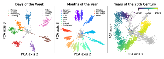
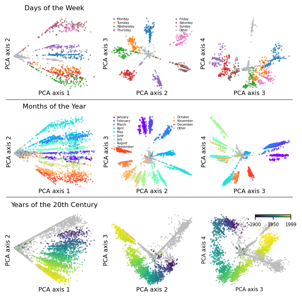
For GPT-2-small, we perform spectral clustering on the roughly 25k layer 7 SAE features from [5], using pairwise angular similarities between dictionary elements as the similarity matrix. We use and manually looked at roughly 500 of these clusters. For each cluster, we looked at projections onto principal components 1-4 of the reconstructed activations for these clusters. In Fig. 12, we show projections for the most interesting clusters we identified, which appear to be circular representations of days of the week, months of the year, and years of the 20th century.
F.2 Mistral 7B methods and results
For Mistral 7B, our SAEs have 65536 dictionary elements and we found it difficult to run spectral clustering on all of these at once. We therefore develop a simple graph based clustering algorithm that we run on Mistral 7B SAEs:
-
1.
Create a graph out of the dictionary elements by adding directed edges from each dictionary element to its closest dictionary elements by cosine similarity. We use .
-
2.
Make the graph undirected by turning every directed edge into an undirected edge.
-
3.
Prune edges with cosine similarity less than a threshold value . We use .
-
4.
Return the connected components as clusters.
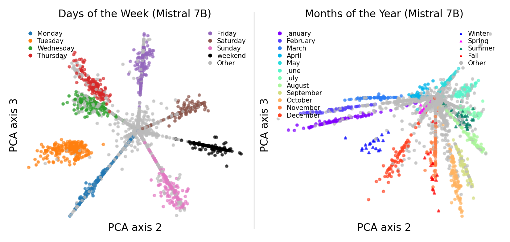
We run this algorithm on the Mistral 7B layer SAE ( dictionary elements) and find roughly clusters containing between and elements. We manually inspected roughly 2000 of these. From these, we re-discover circular representations of days of the week and months of the year, shown in Fig. 13. However, we did not find other obviously interesting and clearly irreducible features.
As future work, we think it would be exciting to develop better clustering techniques for SAE features. Our graph based clustering technique could likely be improved by more recent efficient and high-quality graph based clustering techniques, e.g. hierarchical agglomerate clustering with single-linkage [25]. Additionally, we believe we would see a large improvement by setting edge weights to be a combination of both the cosine and Jaccard similarity of the dictionary elements, e.g. max(cosine, Jaccard).
Appendix G Further Experiment Details
G.1 Assets Information
We use the following open source models for our experiments: Llama 3 8B [2] (custom Llama 3 license https://llama.meta.com/llama3/license/), Mistral 7B [21] (released under the Apache 2 License), and GPT-2 [41] (modified MIT license, see https://github.com/openai/gpt-2/blob/master/LICENSE).
G.2 Machine Information
Intervention experiments were run on two V100 GPUs using less than GB of CPU RAM; all experiments can be reproduced from our open source repository in less than a day with this configuration. We use the TransformerLens library [34] for intervention experiments. -mixture index measurements on toy datasets took about one minute each, on 8GB of CPU RAM. EVR experiments take seconds on 8GB of CPU RAM and are dominated by time taken to human-interpret the RGB plots.
GPT-2 SAE clustering and plotting was run on a cluster of heterogeneous hardware. Spectral clustering and computing reconstructions + plotting was done on CPUs only. We made reconstruction plots for 500 clusters, with each taking less than 10 minutes. Mistral 7B SAE reconstruction plots were made on the same cluster. We made roughly 2000 reconstruction plots for Mistral 7B (and manually inspected each), with each taking less than 20 minutes to generate. Jobs were allocated 64GB of memory each.
Mistral SAE training was run on a single V100 GPU. Initially caching activations from Mistral 7B on one billion tokens took approximately 60 hours. Training the SAEs on the saved activations took another 36 hours.
G.3 Error Bar Calculation
In Fig. 5 we report 96% error bars for all intervention methods. To compute these error bars, we loop over all intervention methods and all layers and compute a confidence interval for each (method, layer) pair across all prompts. Assuming normally distributed errors, we compute error bars with the following standard formula:
where is the sample mean, is the z score (slightly larger than for 96% error bars), and is the standard error (the standard deviation divided by the square root of the number of samples). We use standard Python functions to compute this value.
The reason that the Months error bars are smaller than the Weekdays error bars is because there are more Months prompts: there are intervention effect values, rather than intervention effect values.
Appendix H More Weekdays and Months Plots and Details
We show the results of Mistral 7B and Llama 3 8B on all individual instances of Weekdays that at least one of the models get wrong in Table 2 and present a similar table for Months in Table 3.
We show projections onto the top two PCA directions for both Mistral 7B and Llama 3 8B in Fig. 14 on the hidden layers on top of the token, colored by . These are similar plots to Fig. 3, except they are on all layers. The circular structure in is visible on many—but not all—layers. Much of the linear structure visible is due to .
In Fig. 15 and Fig. 16, we report MLP and attention head patching results for Weekdays and Months. We experiment on 20 pairs of problems with the same and different and 20 pairs of problems with the same and different , for a total of 40 pairs of problems. For each pair of problems, we patch the MLP/attention outputs from the "clean" to the "dirty" problem for each layer and token, and then complete the forward pass. Defining the logit difference as the logit of the clean minus the logit of the dirty , we record what percent of the difference between the original logit difference of the dirty problem and the logit difference of the clean problem is recovered upon intervening, and average across these percentages for each layer and token. This gives us a score we call the Average Intervention Effect.
For simplicity of presentation, we clip all of the (few) negative intervention averages to (prior work [48] has also found negative-effect attention heads during patching experiments).
| Ground truth | Mistral top | Mistral correct? | Llama top | Llama correct? | ||
|---|---|---|---|---|---|---|
| 1 | 1 | Wednesday | Wednesday | Yes | Thursday | No |
| 3 | 1 | Friday | Friday | Yes | Tuesday | No |
| 4 | 1 | Saturday | Saturday | Yes | Thursday | No |
| 3 | 2 | Saturday | Saturday | Yes | Tuesday | No |
| 4 | 2 | Sunday | Sunday | Yes | Wednesday | No |
| 5 | 2 | Monday | Monday | Yes | Tuesday | No |
| 2 | 3 | Saturday | Friday | No | Saturday | Yes |
| 3 | 3 | Sunday | Sunday | Yes | Tuesday | No |
| 4 | 3 | Monday | Monday | Yes | Tuesday | No |
| 0 | 4 | Friday | Thursday | No | Friday | Yes |
| 3 | 4 | Monday | Monday | Yes | Tuesday | No |
| 0 | 5 | Saturday | Friday | No | Saturday | Yes |
| 1 | 5 | Sunday | Saturday | No | Wednesday | No |
| 2 | 5 | Monday | Sunday | No | Monday | Yes |
| 4 | 5 | Wednesday | Tuesday | No | Tuesday | No |
| 6 | 5 | Friday | Thursday | No | Thursday | No |
| 1 | 6 | Monday | Sunday | No | Thursday | No |
| 2 | 6 | Tuesday | Monday | No | Tuesday | Yes |
| 3 | 6 | Wednesday | Tuesday | No | Tuesday | No |
| 4 | 6 | Thursday | Thursday | Yes | Tuesday | No |
| 5 | 6 | Friday | Friday | Yes | Thursday | No |
| 6 | 6 | Saturday | Thursday | No | Thursday | No |
| 0 | 7 | Monday | Sunday | No | Tuesday | No |
| 1 | 7 | Tuesday | Sunday | No | Tuesday | Yes |
| 2 | 7 | Wednesday | Sunday | No | Wednesday | Yes |
| 3 | 7 | Thursday | Sunday | No | Thursday | Yes |
| 4 | 7 | Friday | Thursday | No | Tuesday | No |
| 5 | 7 | Saturday | Friday | No | Saturday | Yes |
| 6 | 7 | Sunday | Friday | No | Thursday | No |
| Ground truth | Mistral top | Mistral correct? | Llama top | Llama correct? | ||
|---|---|---|---|---|---|---|
| 0 | 4 | May | April | No | May | Yes |
| 6 | 4 | November | October | No | November | Yes |
| 0 | 6 | July | June | No | July | Yes |
| 0 | 7 | August | July | No | August | Yes |
| 1 | 7 | September | October | No | September | Yes |
| 3 | 7 | November | October | No | November | Yes |
| 5 | 7 | January | December | No | January | Yes |
| 6 | 7 | February | January | No | February | Yes |
| 7 | 7 | March | February | No | March | Yes |
| 9 | 7 | May | April | No | May | Yes |
| 4 | 9 | February | February | Yes | January | No |
| 2 | 10 | January | December | No | January | Yes |
| 8 | 10 | July | June | No | July | Yes |
| 1 | 11 | January | December | No | January | Yes |
| 2 | 11 | February | December | No | February | Yes |
| 3 | 11 | March | February | No | March | Yes |
| 7 | 11 | July | June | No | July | Yes |
| 8 | 11 | August | July | No | August | Yes |
| 9 | 11 | September | August | No | September | Yes |
| 0 | 12 | January | December | No | January | Yes |
Appendix I Further EVR Results
In this section, we present results to support a claim that MLPs (and not attention blocks) are responsible for computing . In Fig. 17, we deconstruct states on top of the final token (before predicting ) on Llama 3 8B Months (we show a similar plot for the states on the final token of Mistral 7B on Weekdays in the main text in Fig. 8. These plots show that the value of is computed on the final token around layers to . To show that this computation of occurs in the MLPs, we must show that no attention head is copying from a prior token or directly computing .
We first perform a patching experiment with the same setup Fig. 16 and Fig. 15 on individual attention heads on the final token. From the patching results we identify the top attention heads by average intervention effect. For each attention head, we compute one EVR run with explanatory functions equal to one-hot functions of and (resulting in functions for Weekdays and for Months) and one with explanatory functions equal to one-hot functions of , , and . We find that for all layers before , adding to the explanatory functions adds almost no explanatory power. Since we established above that the model has already computed at this point, we know that attention heads do not participate in computing .
| L | H | Average Intervention Effect | EVR One Hot , | EVR One Hot , , |
|---|---|---|---|---|
| 28 | 18 | 0.22 | 0.39 | 0.73 |
| 18 | 30 | 0.17 | 0.95 | 0.96 |
| 15 | 13 | 0.17 | 0.94 | 0.95 |
| 22 | 15 | 0.11 | 0.77 | 0.82 |
| 16 | 21 | 0.09 | 0.92 | 0.93 |
| 28 | 16 | 0.08 | 0.42 | 0.69 |
| 15 | 14 | 0.06 | 0.98 | 0.99 |
| 30 | 24 | 0.05 | 0.43 | 0.79 |
| 21 | 26 | 0.04 | 0.53 | 0.63 |
| 14 | 2 | 0.04 | 0.93 | 0.95 |
| L | H | Average Intervention Effect | EVR One Hot , | EVR One Hot , , |
|---|---|---|---|---|
| 17 | 0 | 0.18 | 0.98 | 0.99 |
| 17 | 1 | 0.08 | 0.98 | 0.98 |
| 19 | 10 | 0.08 | 0.95 | 0.96 |
| 30 | 17 | 0.07 | 0.85 | 0.90 |
| 17 | 3 | 0.07 | 0.93 | 0.95 |
| 17 | 27 | 0.06 | 1.00 | 1.00 |
| 31 | 22 | 0.05 | 0.37 | 0.78 |
| 21 | 9 | 0.04 | 0.73 | 0.78 |
| 20 | 28 | 0.04 | 1.00 | 1.00 |
| 30 | 16 | 0.04 | 0.73 | 0.85 |
| L | H | Average Intervention Effect | EVR One Hot , | EVR One Hot , , |
|---|---|---|---|---|
| 20 | 28 | 0.15 | 0.76 | 0.76 |
| 17 | 0 | 0.10 | 0.77 | 0.77 |
| 25 | 14 | 0.08 | 0.19 | 0.61 |
| 17 | 1 | 0.07 | 0.80 | 0.82 |
| 17 | 3 | 0.06 | 0.71 | 0.71 |
| 31 | 22 | 0.06 | 0.12 | 0.67 |
| 17 | 27 | 0.05 | 0.58 | 0.58 |
| 19 | 4 | 0.05 | 0.40 | 0.66 |
| 19 | 10 | 0.04 | 0.62 | 0.62 |
| 30 | 26 | 0.04 | 0.51 | 0.62 |
| L | H | Average Intervention Effect | EVR One Hot , | EVR One Hot , , |
|---|---|---|---|---|
| 15 | 13 | 0.26 | 0.62 | 0.62 |
| 16 | 21 | 0.17 | 0.76 | 0.76 |
| 18 | 30 | 0.13 | 0.77 | 0.77 |
| 28 | 18 | 0.11 | 0.13 | 0.52 |
| 28 | 16 | 0.07 | 0.13 | 0.52 |
| 21 | 25 | 0.05 | 0.65 | 0.70 |
| 15 | 14 | 0.03 | 0.72 | 0.72 |
| 17 | 26 | 0.02 | 0.77 | 0.77 |
| 31 | 1 | 0.02 | 0.11 | 0.57 |
| 21 | 24 | 0.02 | 0.30 | 0.45 |