New limits on neutrino decay from high-energy astrophysical neutrinos 

Abstract

Since neutrinos have mass differences, they could decay into one another. But their lifetimes are likely long, even when shortened by new physics, so decay likely impacts neutrinos only during long trips. This makes high-energy astrophysical neutrinos, traveling for up to billions of light-years, sensitive probes of decay. However, their sensitivity must be tempered by reality. We derive from them thorough bounds on the neutrino lifetimes accounting for critical astrophysical unknowns and the nuances of neutrino detection. Using the diffuse neutrino flux, we disfavor lifetimes $\tau\lesssim 20$–450 s $(m/{\rm eV})$, based on present IceCube data, and forecast factor-of-10 improvements by upcoming detectors. Using, for the first time, neutrinos from the active galaxy NGC 1068, extant unknowns preclude placing lifetime bounds today, but upcoming detectors could disfavor $\tau\sim 100$–5000 s $(m/{\rm eV})$.

I Introduction

The discovery of neutrino oscillations showed that different neutrino states have different masses. This, in turn, implies that they might decay into each other. In minimal extensions of the Standard Model that accommodate massive neutrinos, their lifetime is capped by radiative decays, but is predicted to be vastly longer than the age of the Universe [1, 2, 3], making them effectively stable. However, in non-minimal extensions, neutrinos may decay much faster via new channels [4, 5, 6, 7, 8, 9, 10, 1, 11, 12, 13, 14, 15, 16, 17] and lead to effects that may be detectable within shorter time scales. Thus, looking for neutrino decay may guide us in extending the Standard Model.

A neutrino $\nu_{i}$ might decay into a lighter one, $\nu_{j}$, plus an additional particle, $\Phi$, i.e., $\nu_{i}\to\nu_{j}+\Phi$; we elaborate on this in Sec. III. As a result, in a flux of neutrinos of energy $E_{\nu}$, mass $m_{i}$, and lifetime $\tau_{i}$, the effect of decay a time $t$ after neutrino emission is given by $e^{-\frac{t}{\gamma\tau}}=e^{-\frac{m_{i}}{\tau_{i}}\frac{L}{E_{\nu}}}$, where, because we deal with relativistic neutrinos, $L\approx t$ is their traveled distance and $\gamma\equiv E_{\nu}/m_{i}$, their Lorentz boost. This represents a depletion of the flux due to the disappearance of decaying neutrinos [and its enhancement due to the appearance of daughter neutrinos, which we do not consider (Sec. III)]. Because presently we do not know the values of the neutrino masses, we are sensitive only to the combination $\tau_{i}/m_{i}$, which we refer to below as the “lifetime” (see, however, Ref. [18]).

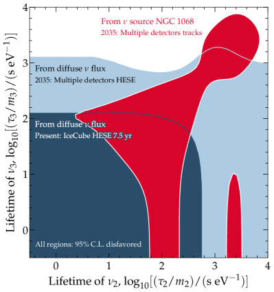
Figure 1: Overview of bounds on neutrino lifetimes from TeV–PeV astrophysical neutrinos. Decay is of the mass eigenstates $\nu_{2}$ and $\nu_{3}$ into invisible products, which modifies the neutrino energy spectrum and flavor composition. Present bounds are from the diffuse neutrino flux, using the IceCube 7.5-year High-Energy Starting Events (HESE) sample; no bound can be placed using present observations of the neutrino source NGC 1068. Forecasts are for 2035 using the combined detection by IceCube and upcoming detectors Baikal-GVD, IceCube-Gen2, KM3NeT, P-ONE, TAMBO, and TRIDENT. In this figure, the bounds are obtained using baseline astrophysical assumptions; Figs. 5 and 6 show alternatives. Bounds derived from the diffuse flux are robust to uncertainty in astrophysical modeling (Fig. 6), but bounds derived from a point neutrino source are strongly impacted by it (Fig. 5).

Upon detection, a significant fraction of $\nu_{i}$ will have decayed if $\tau_{i}/m_{i}\lesssim L/E_{\nu}$. Although neutrino decay remains unobserved, neutrino lifetimes have been constrained by searches using neutrinos from natural and human-made sources [19, 20, 21, 22, 23, 24, 25, 26, 27, 28, 29, 30, 31] that look for signs of decay in the neutrino energy spectrum and flavor composition, i.e., the proportion of $\nu_{e}$, $\nu_{\mu}$, and $\nu_{\tau}$ in an observed flux of neutrinos. In neutrino experiments with terrestrial-scale baselines, of up to a few thousand km, significant time dilation of the neutrino lifetime in the laboratory frame limits our sensitivity to $\lesssim 10^{-10}$ s eV ^-1 [22, 24].

Astrophysical neutrinos overcome this limitation by virtue of their longer baselines. Solar neutrinos, with MeV-scale energies and a baseline of 1 A.U., probe lifetimes of around $5\cdot 10^{-4}$ s eV^-1 [32, 33]. Neutrinos from supernova SN 1987A [34, 35, 36], with tens of MeV and a baseline of $50$ kpc, probe lifetimes of around $5\cdot 10^{5}$ s eV^-1 (though they are subject to model uncertainties) [37, 31].

The IceCube discovery [38] of neutrinos with TeV–PeV energies and Mpc–Gpc baselines has allowed us to probe lifetimes of $\tau_{i}/m_{i}\sim 10^{3}(L/{\rm Gpc})(100~{}{\rm TeV}/E_{\nu})$ s eV^-1, matching or outperforming the above searches. Yet, so far, as pointed out by Ref. [39], searches for neutrino decay with high-energy astrophysical neutrinos [40, 39, 41] have been hampered, implicitly or explicitly, by severely incomplete information on the neutrino properties, source properties, and detection aspects. The presence of these uncertainties, often overlooked, have made it difficult to assess how robust are the bounds on the neutrino lifetime derived from high-energy astrophysical neutrinos.

As high-energy neutrino physics matures, the above limitations weaken. But, more importantly, our ability to quantify their impact on searches for neutrino decay—and searches for other new physics—grows. Recent years have seen improvement in our knowledge of neutrino properties—masses and mixing parameters—a growing number of detected high-energy neutrinos, and improvement in reconstruction techniques. Today, significant uncertainties still affect the searches for decay, but, compared to earlier studies, we are better equipped to assess their impact thanks to the above developments and to the public availability of experimental neutrino data and detailed detector simulations.

Motivated by this, we revisit neutrino decay with high-energy astrophysical neutrinos from a fresh perspective. We provide new limits on neutrino lifetimes; arguably, these are the most robust limits based on high-energy astrophysical neutrinos to date. But our goal is broader: to show the manifest impact of present-day unknowns, the realistic opportunities made possible by spectacular recent discoveries—notably, of the first steady-state high-energy astrophysical neutrino source, NGC 1068 [42]—and the near-future reach of new detectors.

The rest of this paper is organized as follows. In Sec. II we outline the new perspectives of our work. In Sec. III we discuss the phenomenological impact of neutrino decay on the observed neutrino spectrum and flavor composition. In Sec. IV, we discuss the bounds that can be set using the neutrino signal from NGC 1068, and in Sec. V we obtain bounds from the diffuse neutrino flux. Finally, in Sec. VI we summarize and discuss our results.

II Synopsis

In contrast to previous searches for neutrino decay that use high-energy astrophysical neutrinos, ours embraces hitherto unexplored or partially explored uncertainties and model neutrino detection in a realistic way:

Astrophysical uncertainties

Because the bulk of the sources and the production mechanisms of high-energy astrophysical neutrino are unknown, large uncertainties in the predictions of the neutrino flux cloud the presence of potential features introduced by neutrino decay. We explore the impact on the sensitivity to decay of unknowns in the size of the emitted neutrino flux, its energy spectrum, flavor composition, the distribution of neutrino sources, and the number of source populations.

Detailed neutrino detection

The precision with which high-energy neutrino telescopes infer the energy, direction, and flavor of detected neutrinos limits our capability to spot potential features introduced by neutrino decay. To account for this, we model high-energy neutrino detection in as much detail as is publicly accessible, including energy and direction resolution, in-Earth propagation effects, and backgrounds of atmospheric neutrinos and muons. We use Monte Carlo event samples provided by the IceCube Collaboration when available [43] (i.e., for the diffuse flux below), and third-party approximations otherwise [44] (i.e., for the point-source flux below).

The impact of the above perspectives on the sensitivity to decay ranges from appreciable to critical. They render our results realistic, but also weaken them; in some cases—in particular, for neutrinos from an identified source (see below)—to the point of nearly eliminating sensitivity to neutrino decay altogether. We elaborate on the above perspectives later.

We apply these perspectives along two fronts:

Diffuse neutrino flux

We revisit tests of neutrino decay that use the diffuse flux of high-energy astrophysical neutrinos, i.e., the aggregated flux from all unresolved sources. So far, they had been only estimated in Ref. [39] (see also Refs. [45, 46, 47, 48, 49, 50, 51, 52, 53, 54, 55, 56, 57, 58, 40]). For the first time, we report bounds on the neutrino lifetime from the diffuse neutrino flux rigorously derived from a nuanced detector description. We look for signs of decay jointly in the energy spectrum and the flavor composition of the neutrino flux, as proposed by Ref. [40].

Point-source neutrino flux

Recently, IceCube discovered the first steady-state astrophysical candidate source of high-energy neutrinos, the active galaxy NGC 1068 [42], located 14 Mpc away. Unlike previously reported transient candidate sources [59, 60, 61, 62], the number of neutrinos detected from NGC 1068 is a few tens, enough to make it plausible to search for the energy-dependent features characteristic of neutrino decay (Sec. III). Given the angular resolution with which IceCube detects neutrinos from NGC 1068—and from any other possible extragalactic neutrino source—it is effectively a point source. For the first time, we search for signs of decay in the neutrinos from NGC 1068. We do so using only their energy spectrum, since their flavor composition has not yet been measured (see, however, Ref. [63]).

We report bounds on neutrino lifetime based on present-day observations by IceCube and on projected observations by its combination with upcoming or planned neutrino telescopes Baikal-GVD [64], IceCube-Gen2 [65]—the envisioned high-energy upgrade of IceCube—KM3NeT [66], P-ONE [67], TAMBO [68] , and TRIDENT [69]. We expand on them later.

Figure 1 shows an overview of our present-day and projected bounds obtained under baseline model choices. We defer details about them to Secs. IV and V. We consider the non-radiative decay of the mass eigenstates $\nu_{2}$ and $\nu_{3}$ into $\nu_{1}$, which we assume to be the lightest one, plus an undetectable partner. As we discuss below (Sec. III.1), we focus as a benchmark on invisible decay, where the daughter $\nu_{1}$ is also undetectable.

Presently, the diffuse neutrino flux constrains the lifetimes to be smaller than a few times 100 s eV^-1. Future combined detection by multiple detectors in the year 2035 could improve this by one order of magnitude for $\nu_{3}$, assuming that the real flavor composition is the one suggested by present-day data (more on this later). The projected bounds from diffuse flux are robust: they are weakened by adopting alternative model choices within the breadth of astrophysical uncertainties, but do not vanish.

In contrast, present observations of NGC 1068 cannot constrain the neutrino lifetime, but Fig. 1 shows that future observations may probe lifetimes of $10^{3}$–$10^{4}$ s eV^-1, beyond the reach of the bounds from the diffuse flux. However, we find that this is true only under favorable model choices, like those made in Fig. 1. Under most other model choices within the breadth of astrophysical uncertainties the projected lifetime bounds from NGC 1068 vanish or nearly vanish.

The above general observations, which we expand upon below, illustrate a larger point: for searches for physics beyond the Standard Model that use high-energy astrophysical neutrinos to be robust, they must be tempered by realistic astrophysical uncertainties.

III Decay in high-energy astrophysical neutrinos

III.1 Overview of invisible neutrino decay

If neutrinos are unstable, high-energy neutrinos emitted by an astrophysical source may decay on their way to Earth. If the decay is significant, i.e., if the neutrino lifetimes are sufficiently short, it may modify the energy spectrum and flavor composition of the neutrino flux that reaches Earth. Below, we describe these modifications; later (Secs. IV and V), we look for evidence of them.

The magnitude of the modifications introduced by decay depends on the size of the neutrino lifetime, $\tau_{i}/m_{i}$, relative to $L/E_{\nu}$ (Sec. I), but their specific form depends on how neutrinos decay. We focus on the case of “invisible decay”, where neutrinos decay to particles that are undetected by high-energy neutrino telescopes, e.g., low-energy neutrinos or non-standard particles like Majorons and sterile neutrinos. This is not the most general decay scenario, but it is a useful benchmark, since it captures the essential features of decay and allows us to clearly show the impact of the new perspectives introduced in Sec. II. We comment on alternative scenarios later.

We consider three active neutrino flavor states, $\nu_{e}$, $\nu_{\mu}$, and $\nu_{\tau}$, each a superposition of the neutrino mass eigenstates $\nu_{1}$, $\nu_{2}$, and $\nu_{3}$, i.e., $\nu_{\alpha}=\sum_{i=1}^{3}U_{\alpha i}^{\ast}\nu_{i}$, ($\alpha=e,\mu,\tau$ and $i=1,2,3$), where $U_{\alpha i}$ are elements of the Pontecorvo-Maki-Nakagawa-Sakata (PMNS) mixing matrix [70, 71]. It is the mass eigenstates that decay, since, unlike flavor states, they have a well-defined mass. We explore the invisible decay of $\nu_{2}$ and $\nu_{3}$, while keeping $\nu_{1}$ stable. This is motivated by the present mild preference for the normal neutrino mass ordering, where $\nu_{1}$ is the lightest of the mass eigenstates, but there are other possible decay channels [72, 28]. (The scenario in which $\nu_{1}$ is unstable is constrained by the observation of neutrinos from supernova SN 1987A [31]. An unstable $\nu_{1}$ demands a total energy emitted in neutrinos larger than seen in even the most optimistic supernova simulations [73].)

In the more general case of “visible decay”, which we do not explore, the heavier neutrino mass eigenstates decay into the lightest one, e.g., $\nu_{2},\nu_{3}\to\nu_{1}+\Phi$, where $\nu_{1}$ is detectable and $\Phi$ is, in general, not. The effect of decay on the neutrino energy spectrum depends on the fraction of the parent neutrino energy received by the daughter neutrino, and the flavor composition at Earth depends on the mass differences between parent and daughter neutrinos; see, e.g., Refs. [39, 28]. We also do not consider the possibility of chains of decay, e.g., $\nu_{3}\to\nu_{2}+\Phi$ followed by $\nu_{2}\to\nu_{1}+\Phi$; see Ref. [28] for a full treatment. The conclusions that we draw later under invisible decay apply to neutrino decay generally, though the values of the limits on neutrino lifetime that we obtain do not.

The effects introduced by the decay of $\nu_{2}$ and $\nu_{3}$ depend on the factors $e^{-\frac{\tau_{2}}{m_{2}}\frac{L}{E_{\nu}}}$ and $e^{-\frac{\tau_{3}}{m_{3}}\frac{L}{E_{\nu}}}$ (Sec. I). Below, we show how they modify the flavor composition (Sec. III.2) and energy spectrum (Sec. III.4) of high-energy astrophysical neutrinos.

III.2 Neutrino decay in the flavor composition

The mechanism by which high-energy neutrinos are produced determines the flavor composition with which they are emitted, i.e., the proportion of $\nu_{e}$, $\nu_{\mu}$, and $\nu_{\tau}$ in their emitted flux. Because neutrinos oscillate on their way to Earth, the flavor composition of the flux that reaches Earth is different from the one at production. And if, in addition, neutrinos decay along the way, their flavor composition at Earth might deviate from the standard-oscillation expectation [57].

Neutrino production.—Sources of high-energy astrophysical neutrinos are believed to produce them in interactions of high-energy protons with ambient matter or radiation (Sec. IV). Both types of interaction produce high-energy charged pions—and other products—that, upon decaying, produce high-energy neutrinos.

Pions decay via $\pi^{+}\to\mu^{+}\nu_{\mu}$ followed by $\mu^{+}\to\overline{\nu}_{\mu}\nu_{e}e^{+}$, and their charge-conjugated processes. Thus, sources (S) where this decay chain develops in full emit neutrinos with a pion-beam flavor composition of $(f_{e},f_{\mu},f_{\tau})_{\rm S}=(\frac{1}{3},\frac{2}{3},0)$, where $f_{\alpha,{\rm S}}$ is the fraction of $\nu_{\alpha}+\bar{\nu}_{\alpha}$ in the flux. In sources that harbor strong magnetic fields, the intermediate muons may cool via synchrotron radiation, so that, their energies dampened, the neutrinos they decay into are high-energy no more. This yields a muon-damped flavor composition of $(0,1,0)_{\rm S}$. Finally, towards low energies, $\bar{\nu}_{e}$ from the beta-decay of neutrons co-produced with the pions could yield a neutron-beam flavor composition of $(1,0,0)_{\rm S}$.

We adopt the pion-beam, muon-damped, and neutron-beam scenarios as benchmarks in our analysis. They—and all standard neutrino production scenarios—share $f_{\tau,{\rm S}}=0$, since $\nu_{\tau}$ production has a large threshold center-of-mass energy to produce the taus from whose decays $\nu_{\tau}$ would be emitted. There are other possibilities for the flavor composition emitted by the sources, including their evolving with neutrino energy, that depend, e.g., on the geometry and density of the sources and the energies reached by protons and other nuclei inside them; see, e.g., Refs. [74, 75, 76, 77, 78, 79, 80, 81, 82, 83]. In our analysis, rather than exploring them individually, we consider generic scenarios of flavor composition that capture the uncertainty in $f_{\alpha,{\rm S}}$.

Flavor composition at Earth.—As a result of neutrino oscillations, the flavor composition at Earth ($\oplus$) is, for a given choice of $f_{\alpha,{\rm S}}$,

$$f_{\alpha,\oplus}=\sum_{\beta=e,\mu,\tau}\left(\sum_{i=1}^{3}\left|U_{\beta i}\right|^{2}\left|U_{\alpha i}\right|^{2}\right)f_{\beta,{\rm S}}\;,$$ (1)

where the term in parentheses is the average probability of the flavor transition $\nu_{\beta}\to\nu_{\alpha}$, computed for high-energy astrophysical neutrinos (see, e.g., Refs. [84, 81, 29, 85]). The PMNS matrix elements depend on three mixing angles, $\theta_{12}$, $\theta_{23}$, and $\theta_{13}$, and one CP-violation phase, $\delta_{\rm CP}$, whose values are known from oscillation experiments to different degrees of precision. In our analysis, we use their best-fit values and allowed ranges from the recent NuFIT 5.2 global fit to oscillation data [86, 87], obtained assuming normal neutrino mass ordering. (Using instead the values obtained under inverted ordering would not change our results significantly; see, e.g., Ref. [57].)

Figure 2 shows the flavor composition at Earth corresponding to our three benchmark scenarios, computed assuming the present-day best-fit values of the mixing parameters. The nominal expectation, from the pion-beam scenario, yields approximately equal proportion of each flavor at Earth, i.e., roughly $\left(\frac{1}{3},\frac{1}{3},\frac{1}{3}\right)_{\oplus}$.

Figure 2 also shows the theoretically palatable region of flavor composition at Earth [57] (see also Refs. [47, 88, 89, 90]). This is the region of flavor composition generated by simultaneously varying the values of the mixing parameters within their allowed ranges and the flavor composition at the sources as $(f_{e,{\rm S}},f_{\mu,{\rm S}}\equiv 1-f_{e,{\rm S}},f_{\tau,{\rm S}}=0)$, with $0\leq f_{e,{\rm S}}\leq 1$. As stated in Ref. [57], the length of the long axis of the region is due mainly to the variation in $f_{e,{\rm S}}$, and also to the uncertainty in $\theta_{23}$ and $\delta_{\rm CP}$; the length of the short axis is due to the uncertainty in $\theta_{12}$. The effect of the uncertainty in $\theta_{13}$ is tiny. (Allowing $f_{\tau,{\rm S}}\neq 0$ enlarges the region only marginally [57].)

Figure 2: Flavor composition of high-energy astrophysical neutrinos at Earth under the effects of neutrino decay. The regions of allowed flavor composition are generated by exploring all possible flavor combinations at the sources assuming no $\nu_{\tau}$ production, i.e., $(f_{e,{\rm S}},f_{\mu,{\rm S}}=1-f_{e,{\rm S}},f_{\tau,{\rm S}}=0)$, and accounting for present-day uncertainty on the neutrino mixing parameters, from NuFIT 5.2 [86, 87]; see also Refs. [57, 40, 39, 91, 89, 90]. Separate regions are for the standard case of no neutrino decay, invisible decay of $\nu_{2}$ only, of $\nu_{3}$ only, and of both, in all cases into $\nu_{1}$ and an undetected partner. For comparison, we show expectations for three benchmark production scenarios—pion decay, muon-damped pion decay, and neutron decay—and the latest flavor measurement by IceCube [92]. Because the region of flavor composition under complete decay of $\nu_{2}$, or of $\nu_{2}$ and $\nu_{3}$, is clearly separated from the standard region and near the edge of the IceCube measured region, our analysis (Sec. V) using the present-day diffuse neutrino flux already disfavors it.

Today, the uncertainties in the values of the mixing parameters are small enough to render the theoretically palatable region relatively small, about 10% of the flavor triangle in Fig. 2. However, they are still sizable enough to confound effects of neutrino decay, as we show next.

The flavor composition is a versatile probe of neutrino astrophysics and fundamental physics. For astrophysics, it reflects the conditions present in the astrophysical neutrino sources and so may help narrow down their identity [93, 94, 95, 47, 48, 96, 75, 97, 98, 76, 99, 100, 77, 101, 102, 103, 57, 104, 105, 106, 107, 89, 108, 109, 110, 111]. For fundamental physics, it probes neutrino mixing and may reveal new physics [46, 47, 48, 112, 49, 113, 97, 76, 114, 99, 100, 115, 116, 117, 52, 72, 53, 118, 54, 119, 120, 121, 88, 57, 56, 40, 122, 123, 39, 91, 124, 125, 126, 127, 128, 129, 130, 131, 132, 133, 134, 89, 135, 136, 109]. Today, the IceCube neutrino telescope regularly measures the flavor composition of high-energy astrophysical neutrinos [137, 138, 139, 140, 141, 142, 92]; we elaborate on this later (Sec. V.2).

Decay in the flavor composition.—The different mass eigenstates, $\nu_{1}$, $\nu_{2}$, and $\nu_{3}$, have different flavor content. The content of $\nu_{\alpha}$ in $\nu_{i}$ is $\left|U_{\alpha i}\right|^{2}$, with the uncertainty on its value due to the uncertainty in the mixing parameters. Roughly, $\nu_{1}$ has 68% of electron flavor in it, $\nu_{2}$ has 30%, and $\nu_{3}$ has 3%, and the remaining flavor content in each is divided equally between muon and tau; see Fig. 1 in Ref. [57], Fig. 2 in Ref. [39], and Fig. 5 in Ref. [89]. Thus, because the invisible decay of $\nu_{2}$ and $\nu_{3}$ changes their abundance relative to $\nu_{1}$, it alters the flavor composition of the high-energy neutrino flux at Earth.

In the extreme case of complete decay of $\nu_{2}$ and $\nu_{3}$ upon reaching Earth, only $\nu_{1}$ remain, and so the flavor composition of the flux is given solely by the flavor content of $\nu_{1}$, i.e., $f_{\alpha,\oplus}=\left|U_{\alpha 1}\right|$, regardless of the flavor composition at the sources. When the decay is incomplete, the flavor composition at the Earth depends on the fraction of remaining $\nu_{2}$ and $\nu_{3}$—which depends on their lifetimes—and on the flavor composition at the sources, which determines their initial abundance. Thus, given that we do not know what are the neutrino lifetimes, we need to understand whether neutrino decay can alter flavor composition in a way that can be distinguished from the standard-oscillation expectation, regardless of the uncertainties in the flavor composition at the sources and the mixing parameters.

Later, we explore this question by detailed calculation of the high-energy neutrino fluxes. Here, we present qualitative insight. We investigate the flavor composition at Earth in four extreme scenarios: (i) no neutrino decay; (ii) $\nu_{2}$ decay completely; (iii) $\nu_{3}$ decay completely; (iv) both $\nu_{2}$ and $\nu_{3}$ decay completely. While the reality might lie in-between these scenarios, they illustrate the origin of our sensitivity to neutrino decay. In each scenario, we generate the region of allowed flavor composition at Earth like before, by considering a generic flavor composition at the sources of $(f_{e,{\rm S}},1-f_{e,{\rm S}},0)$, varying $f_{e,{\rm S}}$ uniformly between $0$ and $1$, and varying the mixing parameters within their presently allowed ranges.

Figure 2 shows the resulting regions. Scenario (i), without decay, yields the standard, theoretically palatable region that we described earlier. Scenario (ii), where only $\nu_{2}$ decay completely, yields a region that fully contains the standard region. Because of the uncertainty in the flavor composition at the sources and in the mixing parameters, a clear separation of scenario (ii) from scenario (i) would be challenging even if a precise measurement of the flavor composition were available. (Future improvements in the precision with which the mixing parameters are known would help [89].)

Scenario (iii), where only $\nu_{3}$ decay completely, yields a region that only partially overlaps the standard region. As a result, a precise measurement of the flavor composition could, in principle, separate (iii) from (i). In particular, if future measurements were to reveal that the flavor composition is either pion-beam or muon-damped, Fig. 2 shows that this would disfavor scenario (iii).

Scenario (iv), where both $\nu_{2}$ and $\nu_{3}$ decay completely, yields a region of flavor composition given by the flavor content of the sole remaining eigenstate, $\nu_{1}$ (see the discussion above). The region is small, separate from the standard region, and near the edge of the present-day region measured by IceCube [92]. This suggests that even present data might probe this scenario. Indeed, later (Sec. V) we find that present observations of the diffuse neutrino flux can already exclude it at 95% C.L.

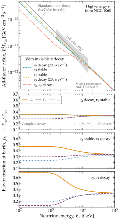
Figure 3: Effect of neutrino decay on the high-energy neutrino flux from NGC 1068. In this figure, we fix the lifetime of decaying neutrinos to a common value of $\tau/m=200$ s eV^-1 as illustration; in our analysis, we vary the lifetime. Top: Neutrino flux at Earth, with and without the effect of $\nu_{2}$ decay, $\nu_{3}$ decay, and both. IceCube measurements are from Ref. [42]. Bottom: Neutrino flavor composition at Earth for the same cases, showing the approximate neutrino energy where neutrino decay becomes important. Neutrino decay induces spectral and flavor distortions within the IceCube energy window; the spectral distortions might disrupt the agreement with precision measurements of the neutrino flux.

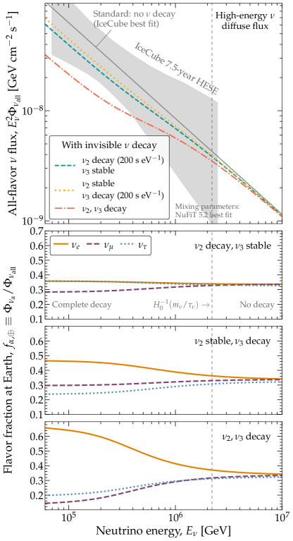
Figure 4: Effect of neutrino decay on the high-energy diffuse neutrino flux. Similar to Fig. 3, but for the diffuse flux of neutrinos detected by IceCube. IceCube measurements are from Ref. [143], based on HESE events. Both the neutrino energy distribution and flavor composition are altered by neutrino decay, providing a potential signature of its existence.

In summary, while testing the decay of only $\nu_{2}$ via the flavor composition is challenging, testing the decay of only $\nu_{3}$, or of $\nu_{2}$ and $\nu_{3}$, has promising prospects, at least from the perspective of theory. Later (Sec. V), we confirm the broad notions presented above via detailed analysis of neutrino observations. However, the main limiting factor to testing neutrino decay via the flavor composition is not the uncertainty in the mixing parameters—which, nevertheless, we account for—but rather the fact that measuring the flavor composition of high-energy astrophysical neutrinos is difficult—which we also account for (Sec. V.2); see also Ref. [89].

III.3 Neutrino decay in the energy spectrum

In our analysis, we constrain neutrino decay using the flux of high-energy neutrinos from a point astrophysical source—specifically, NGC 1068—and from the diffuse flux of high-energy neutrinos. The effect of neutrino decay on the energy spectra is similar in both.

Point-source neutrino flux.—Under neutrino decay, the surviving flux $F_{\alpha}\equiv dN_{\alpha}/(dE_{\nu}dAdt)$ of $\nu_{\alpha}+\bar{\nu}_{\alpha}$ at Earth, per unit energy ($E_{\nu}$), area ($A$), and time ($t)$, emitted by a nearby source,i.e., one located at a distance $r\ll H_{0}^{-1}\approx 4$ Gpc, with $H_{0}$ the Hubble constant, is

$$F_{\alpha}(E_{\nu})=\sum_{\beta,i}\left|U_{\alpha i}\right|^{2}\left|U_{\beta i}\right|^{2}\frac{1}{4\pi r^{2}}\frac{dN_{\beta}}{dE_{\nu}dt}\exp\left[-\frac{m_{i}}{\tau_{i}}\frac{L}{E_{\nu}}\right]\;,$$ (2)

where $dN_{\beta}/dE_{\nu}dt$ is the spectrum of $\nu_{\beta}$ emitted by the source, and the exponential factor reflects the attenuation due to decay (Sec. I). Later, to produce our results (Sec. IV), we use for the emitted spectrum either a power law in $E_{\nu}$, or one augmented by a high-energy cut-off.

Figure 3 shows the neutrino flux from NGC 1068 computed using Eq. (2), assuming for the emitted neutrino spectrum a power law whose normalization and spectral index are fixed to the best-fit values reported by the IceCube Collaboration [42]. For this figure only, as illustration, we assume that the flavor composition at Earth is $\left(\frac{1}{3},\frac{1}{3},\frac{1}{3}\right)_{\oplus}$ in the absence of decay. We show the impact of the invisible decay of $\nu_{2}$ and $\nu_{3}$ on the flux on the all-flavor flux and on the flavor composition, for one choice of value of their lifetime, of 200 s eV^-1, which makes the effects of decay appear within the energy window with which IceCube observes NGC 1068. Later, when generating our results, we vary the lifetimes of $\nu_{2}$ and $\nu_{3}$.

Low-energy neutrinos decay faster because they are less boosted. As a result, the all-flavor flux in Fig. 3 shows that the number of neutrinos drops at energies lower than about $r\cdot\mathrm{max}_{i}(m_{i}/\tau_{i})$. The drop is more pronounced if both $\nu_{2}$ and $\nu_{3}$ decay. The flux transitions from no decay, at high energies, to complete decay, at low energies, over an energy window of about one order of magnitude. The complete decay of $\nu_{2}$ or $\nu_{3}$ removes one third of the flux each; if both decay completely, only a third of the emitted flux survives. If $\nu_{2}$ and $\nu_{3}$ have different lifetimes, their decay could introduce two drops in the flux, at different energies; see, e.g., Ref. [28]. However, because in order for them to be detectable they have to occur within the IceCube energy window, which is rather narrow, and because the transition region is wide, it would be challenging to isolate them.

Figure 3 also shows how neutrino decay alters the flavor composition at Earth as a function of energy. At high energies, the flavor composition is the one expected from standard oscillations in scenario (i) in Sec. III.2. At low energies, if decay is complete, the flavor composition is akin to that expected from scenarios (ii), (iii), or (iv), depending on whether only $\nu_{2}$ decay, only $\nu_{3}$ decay, or both decay. In the transition region, the flavor composition is in-between scenarios (i) and (ii), (iii), or (iv). However, presently, the flavor composition of the neutrinos from NGC 1068 is experimentally inaccessible (Sec. III.4).

Diffuse neutrino flux.—Although the identity, number, and distances to the astrophysical sources responsible for the diffuse neutrino flux are unknown (Sec. V.1), we can estimate it by postulating a population of nondescript sources. We assume that the diffuse flux is due to identical sources whose number density, $\rho_{\rm src}$, evolves with redshift, each source emitting neutrinos with the same spectrum.

Unlike the flux from a nearby point source, the sources that make up the diffuse flux are likely located farther away, at redshifts of $z=1$ or above, i.e., at hundreds of Mpc to a few Gpc. Therefore, we need to account for the effect of the cosmological expansion on the energies of the neutrinos as they propagate to Earth, which changes the size of their Lorentz boost and, as a result, their susceptibility to decay; see Ref. [53] for details.

Under decay, the surviving flux $\Phi_{\alpha}\equiv dN_{\beta}/(dE_{\nu}dAdtd\Omega)$ of $\nu_{\alpha}+\bar{\nu}_{\alpha}$ at Earth, per unit solid angle ($\Omega$), is the sum of contributions from sources across all redshifts [53, 39], i.e.,

$$\Phi_{\alpha}(E_{\nu})=\sum_{\beta,i}\left|U_{\alpha i}\right|^{2}\left|U_{\beta i}\right|^{2}\int_{0}^{\infty}\frac{dz}{H(z)}\rho_{\rm src}(z)$$ (3)

$$\times\frac{dN_{\beta}\left[E_{\nu}(1+z)\right]}{dE_{\nu}dt}\exp\left[-\frac{\tau_{i}}{m_{i}}\frac{1}{E_{\nu}}\int_{0}^{z}\frac{dz^{\prime}}{H(z^{\prime})(1+z^{\prime})^{2}}\right]\;,$$

where $H(z)=H_{0}\left[\Omega_{\Lambda}+(1+z)^{3}\Omega_{m}\right]^{1/2}$ is the Hubble parameter. We assume a $\Lambda$CDM cosmology with $H_{0}=64.7$ km s^-1 Mpc^-1, and adimensional energy density parameters $\Omega_{\Lambda}=0.685$ and $\Omega_{m}=0.315$ [144]. Effectively, contributions from sources at $z\gtrsim 4$ are negligible because they are rare and distant.

Figure 4 shows the diffuse neutrino flux computed using Eq. (3), assuming for the emitted neutrino spectrum a power law whose normalization and spectral index are fixed to the best-fit values reported by the IceCube Collaboration in their analysis of the 7.5-year sample of High-Energy Starting Events (HESE) [143]. As in Fig. 3, for this figure we assume that the flavor composition at Earth is $\left(\frac{1}{3},\frac{1}{3},\frac{1}{3}\right)_{\oplus}$ in the absence of decay. We assume that $\rho_{\rm src}$ follows the star formation rate [145], which places most sources around $z=1$ (more on this later).

Similarly to the point-source neutrino flux, the invisible decay of $\nu_{2}$ and $\nu_{3}$ affects the all-flavor diffuse flux and its flavor composition. Compared to the point-source flux, however, the transition from no decay to complete decay in the diffuse flux is smoothed out, since the sources are located at different redshifts and what we see at Earth is the superposition of the transitions in the individual neutrino spectra they emit. Different from the point-source flux, we do have the capacity at present to measure the flavor composition of the diffuse flux (Sec. III.4).

III.4 Point-source vs. diffuse neutrino fluxes

The neutrinos from NGC 1068 and the diffuse neutrino flux offer complementary sensitivity to neutrino decay:

Different energy ranges

Neutrinos detected from NGC 1068 [42] have lower energies, of roughly 1–10 TeV, than the neutrinos that make up the diffuse flux [143], of roughly 60 TeV–10 PeV. As a result, neutrinos from NGC 1068 have a weaker Lorentz boost (Sec I) and are therefore sensitive to factor-of-10 longer lifetimes.

Different observables

Because neutrinos from NGC 1068 have so far been detected only via $\nu_{\mu}$-initiated muon tracks, with them we can look for the effects of decay solely on the neutrino energy spectrum. In contrast, because the diffuse neutrino flux has been detected using HESE events, which are differently sensitive to all flavors (more on this later), with it we can look for the effects of decay jointly on the energy spectrum and flavor composition.

Comparable uncertainties

Presently, the number of events detected by IceCube from NGC 1068 and from the diffuse flux are roughly comparable (though the former suffers from a higher background). The relative uncertainties with which the flux normalization and spectral index are measured (cf. Refs. [143] and [42]) are comparable between the two fluxes, assuming a power-law neutrino flux.

There is one more subtle difference. The neutrinos from NGC 1068 demonstrably originate from a single source, the distance to which is known. Their energy spectrum is due only to that one source, all neutrinos presumably created in the same processes and under the same physical conditions. Taken at face value, these facts should seemingly reduce the impact of astrophysical uncertainties on the sensitivity to neutrino decay that can be garnered from NGC 1068. In practice, this is not so.

The reason is two-fold. First, because for NGC 1068 we can only look for signs of decay in the all-flavor neutrino energy spectrum—and not also in the flavor composition—the sensitivity is limited to spotting a drop in the flux normalization of, at most, a factor of 3 (Sec. III.3), which is within the uncertainty with which IceCube has measured the flux so far (Fig. 3). Second, there are large theory unknowns in the prediction of the flux, all viable given present experimental uncertainties, that further cloud potential evidence of decay. In our analysis below, we account for both limitations, show how they weaken the sensitivity to neutrino decay significantly, and how in the future they might be mitigated.

In contrast, the diffuse neutrino flux is made up of contributions from an unknown number of unidentified neutrino sources whose distance distribution is also unknown, each one likely producing neutrinos via mechanisms that are at least somewhat different. Taken at face value, these astrophysical uncertainties should render the sensitivity to neutrino decay from the diffuse flux null. In practice, this is not so.

The reason, again, is two-fold. First, even though there is likely an unquantified level of variation in the neutrino spectra and flavor composition emitted by the sources, the diffuse flux that we measure at Earth is their population-averaged aggregate, where presumably this variation has been smoothed out. Second—and more importantly—with the diffuse flux we can look for signs of decay in the flavor composition. Given that the measurement uncertainty of the diffuse flux normalization is comparable to that of NGC 1068—where it is large enough to hide potential signs of decay—it is the flavor composition that delivers the key advantage needed to test neutrino decay.

Below, in Secs. IV and V, we show how the above perspectives are evident in our results.

IV Neutrino lifetime bounds from NGC 1068

We compare the observation of high-energy neutrinos from NGC 1068 against theoretical expectations of the neutrino flux, with and without decay. First we review the salient features of models of astrophysical neutrino production in NGC 1068 and discuss the choices we make for it in our analysis. Then we introduce the statistical procedure we follow to obtain constraints on neutrino decay, and show our results.

IV.1 Astrophysical neutrinos from NGC 1068

Recently, the IceCube Collaboration reported the discovery of an excess of $79_{-20}^{+22}$ neutrinos with about 1–10 TeV from the direction of the active galactic nucleus (AGN) of the Seyfert galaxy NGC 1068 [146, 42], which constitutes an excess over the atmospheric and cosmic background expectations with a statistical significance of $4.2\sigma$. This makes NGC 1068 the first candidate steady-state source of high-energy astrophysical neutrinos.

Neutrino production in NGC 1068.—Although NGC 1068 is likely a high-energy neutrino source, to date it is unclear how and where inside it the neutrinos are made. There are, however, well-motivated hypotheses.

The absence of gamma rays at energies comparable to those of the neutrinos [147] disfavors neutrino production in the outer regions of the galaxy, such as the jet [148], the circumnuclear starburst region [149, 150, 151], a large-scale AGN-driven outflow [152], or an ultra-fast outflow [153].

This suggests that neutrino production occurs in an inner, gamma ray-opaque region [154], which could be the hot AGN corona, where cosmic-ray protons ($p$) and nuclei could undergo neutrino-producing photohadronic ($p\gamma$) interactions on a dense X-ray field [155, 156, 157, 158, 159]. Alternatively, neutrino production in inner regions different from the corona, e.g., the inner circumnuclear region [160], could be dominated by cosmic-ray interactions on surrounding matter ($pp$). In either case, the interactions produce high-energy pions that, upon decaying, produce high-energy neutrinos (Sec. III.2). The specific production channel, and also the cosmic-ray acceleration mechanism, impact the energy spectrum of the neutrinos. Later, we show that the uncertainty in these predictions impacts our sensitivity to neutrino decay.

Already today, neutrino and gamma-ray observations of NGC 1068 provide valuable model-independent constraints on the neutrino spectrum. The IceCube observations [42] show that the neutrino energy flux $E_{\nu}^{2}\Phi_{\nu}$ falls with energy above $1.5$ TeV. Fitting the observations with a power law, $\Phi_{\nu}\propto E_{\nu}^{-\gamma}$, yields a best-fit spectral index $\gamma=3.2$ [42]; see Fig. 3. However, such a soft energy spectrum cannot be extended to arbitrarily low energies, since the electromagnetic emission co-produced with the neutrinos would exceed the bolometric luminosity of the source [154]. Thus, a consistent picture requires a relatively hard neutrino spectrum below about $1$ TeV, with $\gamma<2$, and a softer spectrum at higher energies.

Neutrino flux models.—Broadly stated, the above requirements can be met in two ways. First, it can be obtained by cosmic rays in the source reaching energy equipartition with the magnetic field [159]. This yields a soft power-law neutrino spectrum with $\gamma\approx 3$ across the entire energy range. Second, it can be obtained in models of coronal emission where a change in the spectral index is due to cosmic rays reaching their maximum energy [155, 156, 157, 158]. This yields a neutrino spectrum above 1 TeV that is suppressed by an exponential cut-off $\propto e^{-E_{\nu}/E_{\nu,{\rm cut}}}$, with $E_{\nu,{\rm cut}}$ a characteristic cut-off energy (alternatively, it could also yield a broken power-law spectrum [159]).

In our work, we are only interested in neutrinos above $1$ TeV, where the IceCube observations are presently available. Thus, to reflect the above possibilities, we consider two alternative parametrizations for the energy spectrum: a power law (PL),

$$E_{\nu}^{2}\Phi_{\nu}=(E^{2}_{\nu}\Phi_{\nu})_{0}\left(\frac{E_{\nu}}{1~{}{\rm TeV}}\right)^{2-\gamma}\;,$$ (4)

where the two free parameters are the flux normalization, $(E^{2}_{\nu}\Phi_{\nu})_{0}$, and the spectral index, $\gamma$, and a power law augmented by a cut-off (PC),

$$E_{\nu}^{2}\Phi_{\nu}=(E^{2}_{\nu}\Phi_{\nu})_{0}\left(\frac{E_{\nu}}{1~{}{\rm TeV}}\right)^{2-\gamma}\exp\left(-\frac{E_{\nu}}{E_{\nu,\mathrm{cut}}}\right)\;,$$ (5)

where the three free parameters are $(E^{2}_{\nu}\Phi_{\nu})_{0}$, $\gamma$, and $E_{\nu,\mathrm{cut}}$. Later, we allow the values of these parameters to float. The PC model reproduces the PL model when $E_{\nu,\mathrm{cut}}\gg 15$ TeV, above the range measured by IceCube.

The degeneracy between the PL and PC models reflects the fact that, in the absence of neutrino decay, present-day IceCube observations are described well either by a soft-spectrum PL model, or by a PC model with little sensitivity to the value of the spectral index at energies below the cut-off. In the presence of neutrino decay, the degeneracy allows for more freedom in fitting the observations, and thus yields more conservative bounds on neutrino decay. Our two scenarios, PL and PC, encompass the theoretical possibilities proposed so far to explain the neutrino signal from NGC 1068.

Detecting neutrinos from NGC 1068.—Presently, IceCube observes neutrinos from NGC 1068 exclusively via tracks. These are events where a $\nu_{\mu}$ interacts with a nucleon in the ice and generates a high-energy muon that produces a km-scale track of Cherenkov light as it propagates. The interaction of a $\nu_{\tau}$, and the subsequent decay of the final-state tau, also produces a high-energy muon 17% of the time [144], but this contribution cannot be isolated from that of $\nu_{\mu}$. We expand on neutrino detection in IceCube in Sec. V.2. Because the direction tracks can be reconstructed accurately, typically to less than $1^{\circ}$, they are regularly used to look for point neutrino sources.

The IceCube Collaboration uses a combination of starting and through-going tracks—where the muon is created inside or outside the detector volume, respectively—to infer the energy spectrum of $\nu_{\mu}$ from NGC 1068 (with a small contamination from $\nu_{\tau}$) [42]. In through-going tracks, only a segment of the muon track crosses the detector. This makes inferring the original neutrino energy from the energy deposited by the muon in the ice especially challenging. To make our analysis realistic, when computing event rates (Sec. IV.2), we also combine starting and through-going tracks and account for the uncertainty in the energy reconstruction.

By using exclusively tracks, IceCube is presently unable to measure the flavor composition of the neutrino flux from NGC 1068. This limits our search for neutrino decay to its effects on the energy spectrum (Sec. III.3). Later, we show that this lack of flavor information greatly weakens our sensitivity to neutrino decay.

Yet, although flavor measurements are unavailable, the changes to the $\nu_{\mu}$ spectrum induced by neutrino decay (Sec. III.4) do depend on the flavor composition with which the neutrinos are emitted. Below, we show how.

Flavor composition.—Most models of neutrino production in NGC 1068 predict a pion-beam flavor composition (Sec. III.2), i.e., $\left(\frac{1}{3},\frac{2}{3},0\right)_{\rm S}$. This is a robust prediction. Even in the extreme case where the AGN corona is very compact and the energy densities of the magnetic field and X-rays in it are equal, the magnetic field intensity in the region would be about $10^{4}$ G [159], which would induce a transition to the muon-damped regime only at energies above $100$ TeV [102, 107, 83], well beyond the IceCube range. Hence, we consider as our baseline scenario a pion-beam flavor composition when comparing our predictions to observations, either real or projected.

In addition, we also test a generic scenario with no $\nu_{\tau}$ production and with the form $(f_{e,{\rm S}},1-f_{e,{\rm S}},0)$ (Sec. III.2), where we vary the $\nu_{e}$ fraction, $f_{e,{\rm S}}\in[0,0.5]$ when comparing our predictions to observations. We avoid values of $f_{e,{\rm S}}>0.5$ because they correspond to a neutron-beam composition (Sec. III.2), which is unlikely. If the TeV neutrinos observed by IceCube were produced as $\bar{\nu}_{e}$ in the decay of neutrons created in $pp$ or $p\gamma$ interactions, we would expect associated production of PeV neutrinos from the decay of pions produced in the same interactions, which we have not seen. This generic form of the flavor composition allows us to smoothly shift between the pion-beam and muon-damped benchmarks.

Flux shape and normalization.—In our baseline scenario, we consider the normalization of the neutrino flux and the shape of its energy spectrum from NGC 1068 ($\Phi_{0}$ and $\gamma$ below, respectively) as free parameters, with no prior information on them, i.e., without any associated pull terms in our test statistic (Sec. IV.3). This choice reflects the challenge of our present situation, where, barring adopting an unduly precise prescription of the neutrino flux at emission time, we are confined to looking for signs of decay in the flux at Earth while having little to no knowledge of what it was at emission time, before it could have been affected by neutrino decay.

In the future, this situation could improve by using X-ray observations of NGC 1068. The processes responsible for TeV neutrino production also produce TeV gamma rays that, upon interacting with their environment, cascade down to lower energies and are expected to emerge from the source with MeV-scale energies. Future observations from planned experiments like AMEGO-X [161] and e-ASTROGAM [162], could detect these photons. On the basis of the connection between neutrino and gamma-ray energies, these observations would enable us to estimate the energy in neutrinos emitted by the source, before their decay could possibly affect them. Such estimate would require a detailed understanding of the cascade process and the source environment. For now, it remains as an optimistic future possibility. We entertain it only by proxy by considering an alternative scenario (“tight prior” in Table 1) where we impose a Gaussian prior on the total energy contained in the neutrino flux in the absence of decay, $E_{\nu,{\rm tot}}$, centered at the value of the energy integral of the neutrino flux reported by IceCube [42], with a wide standard deviation of half a decade.

Table 1: Constraints on the neutrino lifetime from the flux of high-energy astrophysical neutrinos from NGC 1068. Constraints are on the lifetimes of $\nu_{2}$ and $\nu_{3}$, computed from projected, cumulative detection of through-going and starting muon tracks by the combination, in PLE$\nu$M [163], of neutrino telescopes Baikal-GVD, IceCube, IceCube-Gen2, KM3NeT, and P-ONE by the year 2035. No constraints can be placed using present-day neutrino observations of NGC 1068 by IceCube alone [42]. The constraints shown are after profiling over all other model parameters, for our eight scenarios of the shape of the neutrino energy spectrum [power law (PL) and power law with high-energy exponential cut-off (PC)], the use of a prior on the neutrino flux normalization (none and tight), and the treatment of the flux composition at the sources, $f_{\rm S}$ (freely floating and fixed to the pion-beam composition). Two-dimensional constraints are preferred because they depict the correlation between $\tau_{2}/m_{2}$ and $\tau_{3}/m_{3}$, which is not captured by the one-dimensional constraints. Blank entries, marked with “$\cdots$”, represent scenarios where no constraint can be placed. See Fig. A2 for a graphical comparison of all one-dimensional constraints and Secs. III and IV for details.

Shape of the neutrino energy spectrum	Prior on the neutrino flux normalization	Neutrino lifetime disfavored at 95% C.L., $\tau_{i}/m_{i}$ [s eV-1] (projected, year 2035, multiple detectors, tracks)
		$f_{\rm S}$ free				$f_{\rm S}$ fixed to $\pi$ decay
		$\frac{\tau_{3}}{m_{3}}$ vs. $\frac{\tau_{2}}{m_{2}}$ (preferred)	$\frac{\tau_{2}}{m_{2}}$	$\frac{\tau_{3}}{m_{3}}$	$\frac{\tau_{2}}{m_{2}}=\frac{\tau_{3}}{m_{3}}$	$\frac{\tau_{3}}{m_{3}}$ vs. $\frac{\tau_{2}}{m_{2}}$ (preferred)	$\frac{\tau_{2}}{m_{2}}$	$\frac{\tau_{3}}{m_{3}}$	$\frac{\tau_{2}}{m_{2}}=\frac{\tau_{3}}{m_{3}}$
PL	None	Fig. 5	$\cdots$	$\cdots$	$[19.63,6382.63]$	Fig. 5	$\cdots$	$\cdots$	$[11.32,7430.19]$
PL	Tight	Fig. 5	$\cdots$	$\cdots$	$[12.56,6839.12]$	Fig. 5	$\cdots$	$\cdots$	$[4.94,7961.59]$
PC	None	Fig. 5	$\cdots$	$\cdots$	$[483.05,1945.36]$	Fig. 5	$\cdots$	$\cdots$	$[365.59,2371.37]$
PC	Tight	Fig. 5	$\cdots$	$\cdots$	$[392.64,2023.02]$	Fig. 5	$\cdots$	$\cdots$	$[283.14,2415.46]$

Table 1 summarizes the eight scenarios that we explore using the neutrino flux from NGC 1068: two alternative shapes of the energy spectrum (PL and PC), two choices for the treatment of the prior on the flux normalization (none and tight), and two choices for the treatment of the flavor composition at the sources (freely floating and fixed to pion-beam). For each scenario, we compute constraints on $\tau_{2}/m_{2}$ and $\tau_{3}/m_{3}$.

IV.2 Computing event rates

Present and projected observations.—So far, IceCube is the only telescope to identify high-energy neutrinos from NGC 1068. We find later (Sec. IV.4) that, in given the large astrophysical unknowns, the present number of IceCube events from NGC 1068—about 80—is insufficient to search for neutrino decay. Fortunately, in the near future, upcoming large-scale neutrino telescopes, currently under construction and planning [136, 29, 164], will boost the detection rate of high-energy neutrinos, including those coming from NGC 1068.

Thus, we perform two separate searches for neutrino decay in the neutrinos from NGC 1068. First, we use the present-day data reported by the IceCube Collaboration in Ref. [42]. Second, we use the combined projected data collected by IceCube and by upcoming ice- and water-Cherenkov neutrino telescopes Baikal-GVD [64], IceCube-Gen2 [65]—the envisioned high-energy upgrade of IceCube—KM3NeT [66], and P-ONE [67]. In all cases, we consider exclusively track events (see, however, Sec. IV.5 for future improvements).

Using PLE$\nu$M to compute detection.—Presently, there are no publicly available resources provided by the IceCube Collaboration to compute with high detail the response of the detector to neutrinos from NGC 1068. [This is different when using HESE events to measure the diffuse neutrino flux (Sec. V).] Hence, we compute event rates using the third-party public code [44] associated to the Planetary Neutrino Monitoring System (PLE$\nu$M) network [163]. PLE$\nu$M is a framework for boosting the information that can be gleamed from the detection of high-energy astrophysical neutrinos by present and future neutrino telescopes, by analyzing their observations within a common computational structure.

The PLE$\nu$M code reproduces the present-day IceCube response to neutrinos from NGC 1068 [42] and, based on it, forecasts the capabilities of future telescopes. It computes neutrino detection by accounting for the effective areas, response functions, and energy and directional resolution of the different detectors listed above. Event rates are computed in terms of the reconstructed muon energy, i.e., the energy of the muon as estimated from the light deposited in the detector by its track. Doing so accounts for the relation between the energy of the parent neutrino, the energy of the muon that it produces, and the experimentally measurable proxy of its energy.

The relation between the neutrino energy and the true muon energy reflects the inelasticity distribution in charged-current neutrino-nucleon interactions, i.e., the distribution of the fraction of neutrino energy that is transferred to the final-state muon. The relation between the true muon energy and reconstructed muon energy is obtained by means of detailed detector simulations. To produce our results, we calibrate it to reproduce the recent improvements that led to the detection of neutrinos from NGC 1068 (Fig. S5 in Ref. [42]). Because the conversion from neutrino energy to reconstructed muon energy smears any features that might exist in the neutrino energy spectrum, such as those induced by neutrino decay (Fig. 3), it muddles their identification.

We bin events in reconstructed muon energy and angular distance from the position of NGC 1068, similarly to Fig. 2 in Ref. [42]. We add to the signal from NGC 1068 the background of tracks due to atmospheric neutrinos and muons, computed, as in Ref. [42], using the Sibyll 2.3c hadronic model for particle interactions and the primary cosmic-ray flux from Ref. [165].

IV.3 Statistical analysis

As discussed above (Sec. IV.1), we consider two scenarios for the energy spectrum of high-energy neutrinos from NGC 1068. In the PL scenario, the spectrum is a power law, determined by the set of astrophysical parameters $\boldsymbol{\theta}_{\rm ast}^{\rm PL}=\left\{\Phi_{0},\gamma,f_{e,{\rm S}}\right\}$, the mixing parameters $\boldsymbol{\theta}_{\rm mix}=\left\{\theta_{12},\theta_{23},\theta_{13},\delta_{\rm CP}\right\}$, and the decay parameters $\boldsymbol{\theta}_{\rm{dec}}=\left\{m_{2}/\tau_{2},m_{3}/\tau_{3}\right\}$. For the PC model, the set of astrophysical parameters is enlarged to account for the cut-off energy, i.e., $\boldsymbol{\theta}_{\rm ast}^{\rm PC}=\left\{\Phi_{0},\gamma,f_{e,{\rm S}},E_{\nu,{\rm cut}}\right\}$.

For each choice of the above parameters, we use the PLE$\nu$M code (Sec. IV.2) to generate the associated event sample, binned in reconstructed muon energy and angular distance from the position of NGC 1068. Similarly to Ref. [42], we use $N_{\hat{E}_{\mu}}=140$ bins in energy, evenly spaced in logarithmic scale between $10^{2}$ and $10^{9}$ GeV, and $N_{\Delta\psi}=225$ bins in angular separation, evenly spaced between 0 and 9 sr. We denote by $\mu_{ij}^{\nu,{\rm ast}}(\boldsymbol{\theta}_{\rm ast},\boldsymbol{\theta}_{\rm mix},\boldsymbol{\theta}_{\rm{dec}},T)$ the mean expected number of tracks induced by the astrophysical neutrino flux from NGC 1068 in the $i$-th energy bin and $j$-th angular bin, computed for the choice of parameters $\boldsymbol{\theta}_{\rm{ast}}$ (either $\boldsymbol{\theta}_{\rm{ast}}^{\rm PL}$ or $\boldsymbol{\theta}_{\rm{ast}}^{\rm PC}$), $\boldsymbol{\theta}_{\rm{mix}}$, and $\boldsymbol{\theta}_{\rm{dec}}$, and for an exposure time $T$.

To account for the contamination of tracks due to the background of atmospheric neutrinos and muons, first, we compute the baseline background event distribution, $N_{ij}^{\mu}(T)$. Then, we keep its spectral and angular shape fixed, but allow for its size to be rescaled by floating its normalization constant, $\mathcal{N}^{\mu}$. Thus, the number of background tracks is $\mu_{ij}^{\rm atm}(\mathcal{N}^{\mu},T)=\mathcal{N}^{\mu}N_{ij}^{\mu}(T)$.

Altogether, the mean number of tracks in each bin, of astrophysical and atmospheric origin, is

$$\mu_{ij}(\boldsymbol{\theta}_{\rm ast},\boldsymbol{\theta}_{\rm mix},\boldsymbol{\theta}_{\rm{dec}},\mathcal{N}^{\mu},T)$$

$$\qquad=\mu_{ij}^{\rm ast}(\boldsymbol{\theta}_{\rm ast},\boldsymbol{\theta}_{\rm mix},\boldsymbol{\theta}_{\rm{dec}},T)+\mu_{ij}^{\mu}(\mathcal{N}^{\mu},T)\;.$$ (6)

As stated above, we perform two analyses: first, using the present-day IceCube observations of NGC 1068 and, second, using projections. We describe them below.

Using present-day data.—We compare the expected number of tracks, $\mu_{ij}$, against the sample of events reported by IceCube [42], in each energy and direction bin, $n_{ij}$. To compare them, we use a binned Poisson likelihood function that spans all bins, i.e.,

$$\ln\mathcal{L}(\boldsymbol{\theta}_{\rm ast},\boldsymbol{\theta}_{\rm{mix}},\boldsymbol{\theta}_{\rm dec},\mathcal{N}^{\mu},T)$$

$$\qquad=\sum_{i=1}^{N_{\hat{E}_{\mu}}}\sum_{j=1}^{N_{\Delta\psi}}\ln\mathcal{L}_{ij,{\rm t}}(\boldsymbol{\theta}_{\rm ast},\boldsymbol{\theta}_{\rm{mix}},\boldsymbol{\theta}_{\rm dec},\mathcal{N}^{\mu},T)$$

$$\qquad\quad+\frac{\chi^{2}(\boldsymbol{\theta}_{\rm{mix}})}{2}+\frac{\chi^{2}(\mathcal{N}^{\mu})}{2}\;,$$

where the likelihood in each bin is

$$\mathcal{L}_{ij}(\boldsymbol{\theta}_{\rm ast},\boldsymbol{\theta}_{\rm{mix}},\boldsymbol{\theta}_{\rm dec},\mathcal{N}^{\mu},T)=\frac{\mu_{ij,\rm t}^{n_{ij,\rm t}}}{n_{ij,\rm t}!}e^{-\mu_{ij,\rm t}}\;,$$ (8)

and, on the right-hand side, $\mu_{ij}\equiv\mu_{ij}(\boldsymbol{\theta}_{\rm ast},\boldsymbol{\theta}_{\rm{mix}},\boldsymbol{\theta}_{\rm dec},\allowbreak\mathcal{N}^{\mu},T)$ is computed using Eq. (IV.3). In Eq. (IV.3), $\chi^{2}(\boldsymbol{\theta}_{\rm{mix}})/2$ and $\chi^{2}(\mathcal{N}^{\mu})/2$ are, respectively, pull terms that represent our prior knowledge of the mixing and atmospheric-background parameters. In our baseline scenario, we do not include pull terms for the astrophysical parameters to avoid introducing bias in our results on the decay parameters. But, in our alternative scenario with a tight prior on the flux normalization, we add a pull term on it, i.e., $\chi^{2}(\Phi_{0})/2$; see Sec. IV.1 and Table 1. For the mixing parameters, we use as priors their distributions from the recent global fit to oscillation data, NuFIT 5.2 [86, 87], assuming normal neutrino mass ordering. For the atmospheric background normalization, we use a flat prior centered on the best-fit value reported in the IceCube analysis [42], and with a width of two decades below and above this value. We tested that using reasonably wider or narrower priors does not affect our results appreciably, as the normalization of the background is constrained well by measurements in sky patches far from NGC 1068.

Since we are only interested in the sensitivity to the decay parameters, we treat the astrophysical, mixing, and atmospheric parameters as nuisance, and profile the likelihood function over them, i.e.,

$$\tilde{\mathcal{L}}(\boldsymbol{\theta}_{\rm dec},T)=\mathrm{max}_{\boldsymbol{\theta}_{\rm ast},\boldsymbol{\theta}_{\rm mix},\mathcal{N}^{\mu}}\mathcal{L}(\boldsymbol{\theta}_{\rm ast},\boldsymbol{\theta}_{\rm{mix}},\boldsymbol{\theta}_{\rm dec},\mathcal{N}^{\mu},T)\;.$$ (9)

We find that the introduction of neutrino decay does not improve the fit to the data. The best-fit value of the decay parameters, $\hat{\boldsymbol{\theta}}_{\rm dec}=\left\{0,0\right\}$, corresponds to no decay of $\nu_{2}$ and $\nu_{3}$. Therefore, we compute lower bounds on the lifetimes $\tau_{2}/m_{2}$ and $\tau_{3}/m_{3}$, i.e., upper bounds on $\boldsymbol{\theta}_{\rm dec}$. We do this via the test statistic

$$\Lambda(\boldsymbol{\theta}_{\mathrm{dec}},T)=2\left[\log\tilde{\mathcal{L}}(\hat{\boldsymbol{\theta}}_{\rm dec},T)-\log\tilde{\mathcal{L}}({\boldsymbol{\theta}_{\rm dec}},T)\right]\;.$$ (10)

By virtue of Wilks’ theorem [166], under the hypothesis that the true decay parameters are $\boldsymbol{\theta}_{\rm dec}$, the test statistic is expected to be distributed as a chi-squared variable with two degrees of freedom, corresponding to the two decay parameters, $(\tau_{2}/m_{2})^{-1}$ and $(\tau_{3}/m_{3})^{-1}$.

Using projected data.—The fundamental limitation in probing the decay of neutrinos from NGC 1068 is that, because they are so far detected only as tracks, we are limited to searching for the relatively small jump in flux normalization that decay could induce (Sec. III.3). This is aggravated by the fact that—at least in our baseline scenario—there is no prior information as to what the flux normalization is before it was possibly affected by decay. Barring gaining access to the flavor composition of the flux from NGC 1068—which we do not consider here (see, however, Ref. [63])—the only way to improve the precision with which decay can be probed in the future is to measure the energy spectrum more precisely.

We explore this scenario by increasing the number of detected events (we mention other possible improvements in Sec. VI). We repeat our analysis above, but now using the cumulative sample of tracks detected, up to the year 2035, collectively by IceCube and upcoming neutrino telescopes Baikal-GVD, IceCube-Gen2, KM3NeT, and P-ONE, each computed within the PLE$\nu$M framework [163] (Sec. IV.2). We scale and rotate the present-day IceCube sensitivity to a neutrino point source in order to simulate the sensitivity of the other telescopes, which have sizes and geographical locations different from IceCube. The total number of detected tracks is the sum of their contributions.

In our projections, we assume for the true $\nu_{\mu}+\bar{\nu}_{\mu}$ flux the best-fit power-law flux reported by IceCube [42], $\Phi_{\nu_{\mu}+\bar{\nu}_{\mu}}=\Phi_{0}[E_{\nu}/(1~{}{\rm TeV})]^{-\gamma}$, with $\Phi_{0}=5\cdot 10^{-14}$ GeV^-1 cm^-2 s^-1 and $\gamma=3.2$, and a pion-beam flavor composition, which allows us to compute the all-flavor flux using the present-day best-fit values of the neutrino mixing parameters. We use Asimov data sets, i.e., we assume that the future observed event rates coincide with the expected rates  [167]. The rest of the analysis proceeds as when using present-day data.

IV.4 Results

Figure 5 shows our resulting two-dimensional joint bounds on the lifetimes of $\nu_{2}$ and $\nu_{3}$, for the scenarios listed in Table 1. This table, and Fig. A2, show also the one-dimensional bounds on the individual lifetimes that, however, discard important correlations between $\tau_{2}/m2$ and $\tau_{3}/m_{3}$, as we explain below.

Using present-day IceCube observations of NGC 1068 it is not possible to constrain neutrino decay. All of the results shown in Fig. 5 are projections, not present-day results. Today, the precision with which the NGC 1068 neutrino spectrum is measured is too poor to spot the step-like factor-of-two-thirds reduction, at most, in the flux normalization that neutrino decay could induce (Fig. 3 and Sec. III.4). This is true in all of our eight analysis scenarios, even in the most optimistic one where we assume a power-law spectrum, fix the flavor composition to pion-beam, and impose a prior on the total neutrino energy emitted.

The above limitation is representative not just of searches for neutrino decay using neutrinos from NGC 1068, but broadly of studies of neutrino physics and astrophysics that rely predominantly on spotting small changes to the normalization of the neutrino flux. Underlying this limitation are the astrophysical unknowns and the insufficient precision of present-day measurements of the neutrino flux. Ignoring either of these aspects would result in unrealistically high sensitivity.

Figure 5 shows that, in the future, it should be possible to constrain the $\nu_{2}$ and $\nu_{3}$ lifetimes, at least under some analysis choices (more on this below). Since our analysis relies on identifying a change in the flux normalization within the energy window in which IceCube observes NGC 1068, our results disfavor lifetimes in the range $L/E_{\nu}\approx 10^{2}$–$10^{3}$ s eV^-1, where $L=14$ Mpc and $E_{\nu}=1$–10 TeV. Neutrino lifetimes below this range would change the flux normalization at energies above the IceCube energy window; lifetimes above this range, at energies below the IceCube energy window. In either case, the transition becomes undetectable and so there is no sensitivity to lifetimes outside the above range.

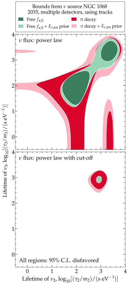
Figure 5: Bounds on the neutrino lifetime using high-energy neutrinos from NGC 1068. All bounds are forecast to the year 2035, from tracks detected by multiple upcoming neutrino telescopes; no bounds can be placed using present IceCube data. Bounds are profiled over all other model parameters, allowing for free flavor composition at the sources (“free $f_{\alpha,{\rm S}}$”), fixing it to pion decay, and possibly constraining the total neutrino energy (“$E_{\nu,{\rm tot}}$ prior”). Top: Assuming a power-law neutrino energy spectrum. Bottom: Assuming a power law with a high-energy cut-off. See Sec. IV for details, Ref. [168] for plot data. Future neutrino lifetime bounds from NGC 1068 hinge on astrophysical unknowns.

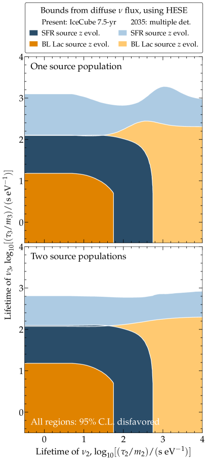
Figure 6: Bounds on the neutrino lifetime using the diffuse flux of high-energy astrophysical neutrinos. Bounds are from HESE events. Present bounds are from the IceCube 7.5-year sample [143, 43]; bounds in the year 2035 are from events detected by multiple upcoming neutrino telescopes. Bounds are profiled over all other model parameters, for two possible choices of the redshift evolution of the source number density: star-formation rate (SFR) and BL Lac. Top: Assuming one source population. Bottom: Assuming two populations. See Sec. V for details, Ref. [168] for plot data. Lifetime bounds from the diffuse flux are sensitive to the redshift distribution of neutrino sources.

Indeed, Fig. 5 shows that, assuming the PL spectrum, if the flavor composition is allowed to float freely and no prior on $E_{\nu,{\rm tot}}$ is adopted, two disconnected regions are excluded, with $\tau_{2}/m_{2}\approx\tau_{3}/m_{3}$ either above $10^{3}$ s eV^-1, or close to $10^{2}$ s eV^-1. However, the projected constraints on neutrino lifetimes based on the neutrinos from NGC 1068 are highly dependent on our analysis choices for the shape of the neutrino spectrum, flavor composition, and the use of a prior on the total energy emitted in neutrinos.

Naturally, fixing the flavor composition to be pion-beam vs. letting it float freely allows us to spot smaller changes to the flux normalization and, therefore, to disfavor larger regions of lifetime. Figure 5 shows that, assuming a PL spectrum, our analysis disfavors lifetimes of $100$ s eV^-1 $\lesssim\tau_{2}/m_{2}\approx\tau_{3}/m_{3}\lesssim 5000$ s eV^-1, where all neutrinos decay below a transition energy in the $1$–$10$ TeV range. In addition, assuming a known flavor composition allows us to exclude the vertical and horizontal regions in Fig. 5 corresponding to $\tau_{2}/m_{2}\simeq 100$ s eV^-1 or $1000$ s eV^-1 while $\tau_{3}/m_{3}\ll 100$ s eV^-1, and vice versa, corresponding to the cases where either $\nu_{2}$ or $\nu_{3}$ decay completely and the decay of the remaining species induces a flux transition within the IceCube energy window. Similarly, adopting a prior on $E_{\nu,{\rm tot}}$ enlarges the region of lifetimes disfavored, since it also allows us to spot smaller changes to the flux normalization.

Figure 5 shows that the largest effect on the lifetime bounds is due to switching between using the PL model vs. the PC models of the neutrino energy spectrum. Our bounds nearly disappear when using the latter model because the high-energy cut-off in the spectrum may mimic the step-like transition in the flux normalization that would be induced by neutrino decay, for some choices of the value of the cut-off energy, $E_{\nu,{\rm cut}}$. Once more, this reflects the critical importance of accounting for astrophysical model uncertainties in searches for new physics.

In our most conservative scenario—adopting the PL model, freely floating flavor composition, and no prior on $E_{\nu,{\rm tot}}$—no lifetime bounds can be drawn. While egregious, this scenario is likely too extreme, and in reality we can likely do better. By fixing instead the flavor composition to pion-beam—as motivated by models of NGC 1068 (Sec. IV.1)—we can exclude $\tau_{2}/m_{2}\approx\tau_{3}/m_{3}\approx 1000$ s eV^-1. This corresponds to a jump in the flux normalization at around $1$ TeV, where it is easier to spot due to the neutrino flux being higher there. While the disfavored region is small, Fig. 1 shows that it is unreachable by searches for neutrino decay based on the diffuse neutrino flux (Sec. V), where neutrino energies are typically higher and so are sensitive to shorter lifetimes.

IV.5 Future improvements

As pointed out earlier, the main limitation to testing neutrino decay using NGC 1068 is that, because today we only observe it via tracks, we are limited to looking for decay-induced features on the neutrino energy spectrum. Combining the detection of tracks—made mainly from $\nu_{\mu}$—and cascades—made by all flavors (Sec. V.2)—from NGC 1068 could circumvent the above limitation by providing an additional probe of neutrino via the flavor composition (Sec. III.2). However, because the pointing resolution of IceCube cascades is significantly worse than that of tracks—of tens of degrees vs. sub-degree—including them in our analysis, today, would come at the cost of using a larger atmospheric neutrino background.

However, the advent of next-generation water-Cherenkov detectors like Baikal-GVD, KM3NeT, P-ONE, and TRIDENT opens up the possibility of observing astrophysical point neutrino sources using also cascades. There, cascades are expected to have a better pointing resolution than in IceCube thanks to the photon scattering length being longer in water than in ice. This would grant us access to tests of neutrino decay using NGC 1068 not only via its neutrino energy spectrum but also via its flavor composition. Reference [63] showed promising preliminary results for this possibility, but an in-depth analysis, possibly using improved flavor-measurement techniques [169, 170, 171], is beyond the scope of the present work.

V Neutrino lifetime bounds from the diffuse neutrino flux

The observation of neutrinos from NGC 1068 cannot at present exclude neutrino decay, but may do so in the future (Sec. IV). In contrast, the observation of the diffuse flux of high-energy astrophysical neutrinos in IceCube can probe neutrino decay already today [45, 46, 47, 48, 49, 50, 51, 52, 53, 54, 55, 56, 57, 58, 40, 39].

The main competitive advantage of using the diffuse flux is that it gives us access not only to the neutrino energy spectrum—like tracks do for NGC 1068—but also to the flavor composition, both of which may be affected by neutrino decay (Sec III.4).

However, because the identity and number of neutrino sources, and the neutrino production mechanism, are unknown, our claims regarding neutrino decay are population-averaged. Below, we explore several representative possibilities spanning the breadth of astrophysical unknowns and show that their influence on our results, while appreciable, is not decisive.

We describe the procedure that we follow to search IceCube data for evidence of neutrino decay, and the constraints on neutrino lifetime that we place. First, we do this for the present-day public 7.5-year public sample of IceCube High-Energy Starting Events (HESE) [143]. Then, we show forecasts based on projected combined measurements by multiple upcoming neutrino telescopes.

V.1 Diffuse high-energy astrophysical neutrino flux

Despite the discovery of the first few sources of high-energy astrophysical neutrinos [59, 61, 62, 42, 172], including NGC 1068, the origin of the bulk of them is unknown. Because the diffuse flux is largely isotropic, the astrophysical sources responsible for it are likely largely extragalactic. They are purportedly cosmic accelerators capable of boosting cosmic-ray protons and nuclei up to energies of at least tens of PeV, and possibly higher [173].

Today, several candidate source classes are under consideration, including active galactic nuclei (AGN), gamma-ray bursts (GRBs), starburst galaxies (SBGs), and galaxy clusters (GCs). Competing theoretical predictions of the neutrino flux from them differ in the specifics, but share a dependence on key factors like the acceleration mechanism, the properties of the ambient matter and radiation with which cosmic rays interact to make neutrinos, and the intensity and configuration of the magnetic fields harbored by the sources. Presently, there is little to no direct experimental information about these properties. Rather than exploring the detailed predictions from competing models, we adopt a phenomenological prescription that captures common features of their energy spectrum and flavor composition.

For the diffuse neutrino spectrum, we adopt a power law, $\Phi_{\nu_{\alpha}}\propto E_{\nu}^{-\gamma}$, where $\gamma>2$; this shape is commonly used in the literature; see, e.g., Refs. [81, 174, 85] and references therein. Using the recent 7.5-year HESE sample—the same one we use (more on this later)—the IceCube Collaboration reported [143] $\gamma=2.87_{-0.19}^{+0.20}$; see Fig. 4. [Other analyses based on different event samples, and covering different but overlapping energy ranges, find harder, but compatible spectra; i.e., through-going muons [175] yield $\gamma=2.37\pm 0.09$, starting tracks [176] yield $\gamma=2.58_{-0.09}^{+0.10}$, and a combined analysis using different types of event samples [141], now somewhat outdated, yields $\gamma=2.50\pm 0.09$ (Ref. [177] has a preliminary update, with comparable results)]. Later, in our statistical analysis based on present-day data, we let the value of $\gamma$ float and be determined by the comparison to real data. When making forecasts, we generate mock event samples by adopting for the true value of $\gamma$ its best-fit value from the 7.5 year HESE analysis [143], and then let its value be determined by the comparison to mock data.

A power-law spectrum is particularly well-motivated in source candidate classes where we expect neutrino production to occur primarily via $pp$ interactions, e.g., SBGs and GCs. In sources where we expect it to occur primarily via $p\gamma$ interactions, e.g., AGN and GRBs, the neutrino spectrum should exhibit a “bump” around a characteristic energy set by the shape of the target photon spectrum; see Fig. 2 in Ref. [174] for an overview. Today, arguably the most convincing argument in favor of choosing to model the neutrino spectrum as a power law vs. choosing alternative, more complex shapes is its consistency with the IceCube observations. Given present-day measurement uncertainties, these alternatives are so far not significantly preferred; see, e.g., Refs. [141, 143, 175, 174, 176].

Thus, we compute the diffuse neutrino flux by considering a population of identical, nondescript astrophysical sources, each one emitting $\nu_{\alpha}+\bar{\nu}_{\alpha}$ with a spectrum

$$\frac{dN_{\alpha}}{dE_{\nu}dt}\propto f_{\alpha,{\rm S}}E_{\nu}^{-\gamma}\;.$$ (11)

We assume that the number density of sources, $\rho_{\rm src}$, evolves with redshift, and compute the diffuse flux at Earth including the effects of neutrino decay, $\Phi_{\nu_{\alpha}}$ in Eq. (3). We treat its all-flavor normalization constant at 100 TeV, $\Phi_{0}$, as a free parameter whose value is determined by observations, real or projected. For the flavor composition at the sources, $(f_{e},f_{\mu},f_{\tau})_{\rm S}$, we assume there is no production of $\nu_{\tau}$, i.e., $f_{\tau,{\rm S}}=0$, like we did for NGC 1068. For our baseline scenario, we consider a single population (1P) of neutrino sources responsible for the diffuse flux, and compute it using Eq. (3).

The diffuse flux that we compute is isotropic, but, in reality, about 10% of the observed diffuse flux comes from the Galactic Plane [172, 178] at tens of TeV. Because neutrinos from the Galactic Plane travel a much shorter path to Earth, the effect of decay on them is weaker than on neutrinos of extragalactic origin, and should be treated separately, or their incoming directions should be masked out. However, in our analysis we assume that all neutrinos are extragalactic, since there is presently no publicly available detailed directional information on the neutrinos detected from the Galactic Plane that we can incorporate in our analysis.

For the redshift evolution of the source number density, we adopt as our baseline assumption the star-formation rate (SFR) [145]. This places most of the sources at redshifts $z\sim 1$, corresponding to a few Gpc, thus lengthening the time of neutrino propagation to Earth and enhancing the potential impact of neutrino decay during it. As a more conservative choice, we also perform an analyses where we adopt a source evolution like that of BL Lac objects, a type of AGN, as extracted from Fig. 5 of Ref. [179] (in turn obtained from Ref. [180]). With it, the source density rapidly falls with redshift, placing more sources closer to Earth.

In addition to the 1P scenario above, we explore the alternative scenario of two contributing populations of neutrino sources (2P), each emitting neutrinos with a different spectrum and flavor composition. We examine whether their interplay leads to features in their combined energy spectrum and flavor composition that could cloud the presence of neutrino decay. The neutrino flux is the superposition of the power-law fluxes from two populations with independent normalization constants $\Phi_{0,1}$ and $\Phi_{0,2}$, spectral indices $\gamma_{1}$ and $\gamma_{2}$, and flavor compositions $f_{\alpha,1}$ and $f_{\alpha,2}$. For simplicity, we use a common source density evolution for both populations.

Table 2 summarizes the eight scenarios that we explore using the diffuse flux for the sensitivity to neutrino decay: two astrophysical production models (1P and 2P), two choices of the source redshift evolution (SFR and BL Lac), and two choices for the treatment of the flavor composition at the sources (freely floating and fixed to pion-beam). For each scenario, we compute constraints on $\tau_{2}/m_{2}$ and $\tau_{3}/m_{3}$.

Table 2: Constraints on the neutrino lifetime from the diffuse flux of high-energy astrophysical neutrinos. The constraints are on the lifetimes of $\nu_{2}$ and $\nu_{3}$, computed using HESE events, using present-day IceCube data and the projected, cumulative detection by the combination of neutrino telescopes Baikal-GVD, IceCube, IceCube-Gen2, KM3NeT, P-ONE, TAMBO, and TRIDENT by the year 2035. The constraints are shown after profiling over all other model parameters, for our eight scenarios of the number of neutrino source populations (1P and 2P), the redshift evolution of their number density (SFR and BL Lac), and the treatment of the flux composition at the sources, $f_{\rm S}$ (freely floating and fixed to the pion-beam composition). Two-dimensional constraints are preferred because they depict the correlation between $\tau_{2}/m_{2}$ and $\tau_{3}/m_{3}$, which is not captured by the one-dimensional constraints. Blank entries, marked with “$\cdots$”, represent scenarios where no constraint can be placed. See Fig. A2 for a graphical comparison of all one-dimensional constraints and Secs. III and V for details.

Number of neutrino source populations

Source density redshift evolution, $\rho_{\rm src}$

Neutrino lifetime disfavored at 95% C.L., $\tau_{i}/m_{i}$ [s eV-1]

Present (7.5-yr IceCube HESE sample)

Projections (year 2035, multiple detectors, HESE)

$f_{\rm S}$ free

$f_{\rm S}$ fixed to $\pi$ decay

$f_{\rm S}$ free

$f_{\rm S}$ fixed to $\pi$ decay

$\frac{\tau_{3}}{m_{3}}$ vs. $\frac{\tau_{2}}{m_{2}}$ (preferred)

$\frac{\tau_{2}}{m_{2}}$

$\frac{\tau_{3}}{m_{3}}$

$\frac{\tau_{2}}{m_{2}}=\frac{\tau_{3}}{m_{3}}$

$\frac{\tau_{2}}{m_{2}}$

$\frac{\tau_{3}}{m_{3}}$

$\frac{\tau_{2}}{m_{2}}=\frac{\tau_{3}}{m_{3}}$

$\frac{\tau_{3}}{m_{3}}$ vs. $\frac{\tau_{2}}{m_{2}}$ (preferred)

$\frac{\tau_{2}}{m_{2}}$

$\frac{\tau_{3}}{m_{3}}$

$\frac{\tau_{2}}{m_{2}}=\frac{\tau_{3}}{m_{3}}$

$\frac{\tau_{2}}{m_{2}}$

$\frac{\tau_{3}}{m_{3}}$

$\frac{\tau_{2}}{m_{2}}=\frac{\tau_{3}}{m_{3}}$

1P

SFR

Fig. 6

$\cdots$

$\cdots$

$\leq$ 219

$\cdots$

$\leq$ 126

$\leq$ 550

Fig. 6

$\cdots$

$\leq$ 1381

$\leq$ 2631

$\cdots$

$\leq$ 1260

$\leq$ 1996

1P

BL Lac

Fig. 6

$\cdots$

$\cdots$

$\leq$ 29

$\cdots$

$\leq$ 20

$\leq$ 105

Fig. 6

$\cdots$

$\leq$ 316

$\leq$ 550

$\cdots$

$\leq$ 316

$\leq$ 501

2P

SFR

Fig. 6

$\cdots$

$\cdots$

$\leq$ 219

$\cdots$

$\leq$ 126

$\leq$ 550

Fig. 6

$\cdots$

$\leq$ 1259

$\leq$ 2400

$\cdots$

$\leq$ 1260

$\leq$ 1996

2P

BL Lac

Fig. 6

$\cdots$

$\cdots$

$\leq$ 26

$\cdots$

$\leq$ 20

$\leq$ 105

Fig. 6

$\cdots$

$\leq$ 316

$\leq$ 182

$\cdots$

$\leq$ 316

$\leq$ 417

V.2 High-Energy Starting Events (HESE)

The measurement of the diffuse flux of high-energy astrophysical neutrinos in IceCube adopts different strategies to mitigate the background of high-energy atmospheric neutrinos. We focus on HESE events [38], i.e., events where the neutrino-nucleon interaction occurs inside the fiducial volume of the detector and the outer layer of photomultiplier strings in the detector is used as a veto to reject the coincident detection of an accompanying muon that would tag an event as being of atmospheric, rather than astrophysical origin [181, 182, 183]. As a result, the samples of HESE events are among the most astrophysically pure ones available, and are therefore well-suited for our purposes.

Compared to the through-going and starting tracks that we used for NGC 1068, HESE events are rare. The public 7.5-year IceCube HESE sample [143, 43] that we use contains 102 detected events between tens of TeV and a few PeV. [A more recent sample [184, 185], using 12 years, contains 164 events. However, because it has no publicly available accompanying sample of Monte Carlo events that we can use in our statistical analysis (more on this later), we use the 7.5-year sample instead.]

At these energies, neutrinos typically interact in the detector via neutrino-nucleon ($\nu N$) deep inelastic scattering. In it, the interacting neutrino scatters off of one of the quarks or gluons of a proton or neutron in the ice, which is broken up into final-state hadrons, $X$, as a result. Interactions can be either neutral-current, when mediated by a $Z$ boson, i.e., $\nu_{\alpha}+N\to\nu_{\alpha}+X$, or charged-current, when mediated by a $W$ boson, i.e., $\nu_{\alpha}+N\to l_{\alpha}+X$. In both cases, the final-state charged particles radiate Cherenkov light that, in IceCube, is picked up by photomultipliers buried in the Antarctic ice. From the amount of light detected, and from its spatial and temporal profiles, it is possible to infer the energy, arrival direction, and, to an extent, the flavor of the interacting neutrino (more on this below).

A HESE event is classified in one of three topologies—cascades, tracks, and double cascades—according to its light profile. Cascades (c) are made primarily by the charged-current interaction of $\nu_{e}$ and $\nu_{\tau}$, where the particle showers triggered by the final-stated hadrons and the final-state electron or tau are superimposed and detected as one. They are also made by the neutral-current interaction of neutrinos of all flavors, although the neutral-current cross section is smaller than the charged-current one. Tracks (t) are made primarily by the charged-current interaction of $\nu_{\mu}$, where the final-state muon leaves a km-scale track of Cherenkov light in its wake that is easily identifiable. They are also made by the charged-current interaction of $\nu_{\tau}$, which generate a tau that decays into a muon about 17% of the time [144]. Double cascades (dc) [186] are made by the charged-current interaction of $\nu_{\tau}$ where a first cascade is produced by the $\nu_{\tau}N$ interaction and a second one, by the hadronic decay of the final-state tau. The majority of detected events are cascades; double cascades are the rarest.

The classification above reveals why it is not possible to firmly infer the flavor of the neutrino in a specific HESE event: a cascade could have been made by a neutrino of any flavor, and a track could have been made by a $\nu_{\mu}$ or a $\nu_{\tau}$. However, as proposed first by Ref. [48], from the relative number of detected events of each topology, IceCube analyses [139, 141, 187, 92] (see also, e.g., Refs. [137, 138, 140, 142]) infer the flavor composition of the neutrino flux, statistically. Thus, HESE events—unlike the through-going [175] or starting tracks [176] from NGC 1068—allow us to look for signs of neutrino decay jointly in the neutrino energy spectrum and flavor composition; see, e.g., Refs. [46, 57, 40, 39]. We comment later on combining measurements of the diffuse flux via HESE events and through-going tracks (Sec. V.6).

V.3 Generating HESE event samples

To accurately model the capability of IceCube to detect high-energy astrophysical neutrinos via HESE events, including the above nuances, we use the Monte Carlo (MC) data sample [43] that is provided by the IceCube Collaboration together with the 7.5-year HESE data release [143]. The MC sample contains a large number of simulated HESE events that were generated using the same detailed detector response used in the analysis of the 7.5-year sample by the IceCube Collaboration. We use it to compute mock samples of detected events for different choices of the neutrino flux, including ones affected by neutrino decay, which we later contrast against the present or projected samples.

The events in the MC sample were generated assuming a reference diffuse high-energy astrophysical neutrino flux [43] of $\Phi_{\alpha,\rm{ref}}=(\Phi_{0,{\rm ref}}/3)(E_{\nu}/100~{}{\rm TeV})^{-2.87}$ for each of three flavors, with $\Phi_{0,{\rm ref}}=5.68\cdot 10^{-18}$ GeV^-1 cm^-2 s^-1 sr^-1, and for an exposure time $T_{\rm ref}=2635$ days. The $k$-th MC event in the sample consists of the flavor, energy, and direction of the simulated neutrino, $\alpha^{k}$, $E_{\nu}^{k}$ and $\cos\theta_{z}^{k}$, respectively, where $\theta_{z}$ is measured with respect to the zenith, and of the event topology (cascade, track, double cascade), reconstructed deposited energy and direction of the ensuing HESE event, t^k, $E_{\mathrm{dep}}^{k}$ and $\cos\theta_{z,\mathrm{rec}}^{k}$, respectively. In addition, the event has an associated reference MC weight $w_{\mathrm{ref}}^{k}$.

To generate a mock sample of HESE events due to an arbitrary diffuse neutrino flux, $\Phi_{\alpha}$, such as the one computed in Eq. (3), and for arbitrary exposure time, $T$, we reweigh the MC events by defining updated weights according to their neutrino energy and flavor, i.e.,

$$w^{k}(E_{\nu}^{k},\alpha^{k})=w^{k}(E_{\nu}^{k},\alpha^{k})\frac{\Phi_{\alpha^{k}}(E_{\nu}^{k})T}{\Phi_{\alpha^{k},\rm{ref}}(E_{\nu}^{k})T_{\rm ref}}\;.$$ (12)

Our analysis uses events binned in $E_{\rm dep}$ and $\cos\theta_{z,\mathrm{rec}}$; we introduce our choice of binning in Sec. V.4. In each bin, the mean expected number of events with topology t is the sum of the weights of MC events with topology t.

As in the 7.5-year HESE analysis by the IceCube Collaboration [143], we include the irreducible background of atmospheric neutrinos and muons (Sec. V.4), and detector systematic uncertainties—the efficiency of digital optical modules, the head-on efficiency, and the lateral efficiency. We keep the latter fixed to their nominal expectations from Ref. [143]. As shown in Ref. [174], doing this has a negligible impact on the reconstructed spectral properties of the flux, and allows us to considerably reduce the computational time needed for our analysis.

V.4 Statistical analysis

Our statistical analysis follows closely the one we used for NGC 1068 in Sec. IV.3. As discussed above (Sec. V.1), we consider two scenarios of neutrino source populations, 1P and 2P. In the 1P scenario, the diffuse neutrino flux from the single source population is determined by the set of astrophysical parameters (Sec. V.1) $\boldsymbol{\theta}_{\rm{ast}}^{1{\rm P}}=\left\{\Phi_{0},\gamma,f_{e,{\rm S}}\right\}$ (since we set the $\nu_{\tau}$ fraction at production to $f_{\tau,{\rm S}}=0$, the $\nu_{\mu}$ fraction is $f_{\mu,{\rm S}}\equiv 1-f_{e,{\rm S}}$), the mixing parameters $\boldsymbol{\theta}_{\rm{mix}}=\left\{\theta_{12},\theta_{23},\theta_{13},\delta_{\rm CP}\right\}$ and the decay parameters $\boldsymbol{\theta}_{\rm{dec}}=\left\{m_{2}/\tau_{2},m_{3}/\tau_{3}\right\}$. For the 2P model, the set of astrophysical parameters is duplicated to account for two populations, i.e., $\boldsymbol{\theta}_{\rm{ast}}^{2{\rm P}}=\left\{\Phi_{0,1},\gamma_{1},f_{e,{\rm S},1},\Phi_{0,2},\gamma_{2},f_{e,{\rm S},2}\right\}$.

For each choice of the above parameters, we use the MC sample (Sec. V.3) to generate the associated event sample, binned in reconstructed energy and direction. Similarly to Refs. [143, 174], we use $N_{E_{\rm dep}}=21$ bins in energy, evenly spaced in $\log_{10}(E_{\rm dep}/{\rm GeV})$, between 60 TeV and 10 PeV, and $N_{c\theta_{z}^{\rm rec}}=10$ bins in direction, evenly spaced in $\cos\theta_{z}^{\rm rec}$, between -1 and 1. We denote by $\mu_{ij,\rm t}^{\nu,\rm{ast}}(\boldsymbol{\theta}_{\rm{ast}},\boldsymbol{\theta}_{\rm{mix}},\boldsymbol{\theta}_{\rm{dec}},T)$ the mean expected number of events with topology t induced by the astrophysical neutrino flux in the $i$-th energy bin and $j$-th angular bin, computed for the choice of parameters $\boldsymbol{\theta}_{\rm{ast}}$ (either $\boldsymbol{\theta}_{\rm{ast}}^{\rm 1P}$ or $\boldsymbol{\theta}_{\rm{ast}}^{\rm 2P}$), $\boldsymbol{\theta}_{\rm{mix}}$, and $\boldsymbol{\theta}_{\rm{dec}}$, and for an exposure time $T$.

To account for the contamination due to the irreducible atmospheric background, first, we extract from the IceCube HESE MC sample [43] the baseline number of conventional atmospheric neutrinos, $N^{\nu,{\rm c}}_{ij,{\rm t}}(T)$, prompt atmospheric neutrinos, $N^{\nu,{\rm pr}}_{ij,{\rm t}}(T)$, and atmospheric muons, $N^{\mu}_{ij,{\rm t}}(T)$. We keep the shape of the background energy and direction event distributions fixed, but allow their normalization constants, $\mathcal{N}^{\nu,{\rm c}}$, $\mathcal{N}^{\nu,{\rm pr}}$, and $\mathcal{N}^{\mu}$, to float independently of each other. Thus, the number of background events of topology t is

$$\mu_{ij,{\rm t}}^{\rm atm}(\boldsymbol{\eta},T) = \mathcal{N}^{\nu,{\rm c}}N^{\nu,{\rm c}}_{ij,{\rm t}}(T)+\mathcal{N}^{\nu,{\rm pr}}N^{\nu,{\rm pr}}_{ij,{\rm t}}(T)$$ (13)

$$+~{}\mathcal{N}^{\mu}N^{\mu}_{ij,{\rm t}}(T)\;,$$

where $\boldsymbol{\eta}\equiv(\mathcal{N}^{\nu,{\rm c}},\mathcal{N}^{\nu,{\rm pr}},\mathcal{N}^{\mu})$.

Altogether, the mean number of events of topology t in each bin, of astrophysical and atmospheric origin, is

$$\mu_{ij,{\rm t}}(\boldsymbol{\theta}_{\rm ast},\boldsymbol{\theta}_{\rm{mix}},\boldsymbol{\theta}_{\rm dec},\boldsymbol{\eta},T) = \mu_{ij,{\rm t}}^{\nu,{\rm ast}}(\boldsymbol{\theta}_{\rm ast},\boldsymbol{\theta}_{\rm{mix}},\boldsymbol{\theta}_{\rm dec},T)$$ (14)

$$+~{}\mu_{ij,{\rm t}}^{\rm atm}(\boldsymbol{\eta},T)\;.$$

Like for NGC 1068 before, we perform two analyses: first, using real HESE data and, second, using projections. We describe them below.

Using present-day data.—We compare the expected number of HESE events of each topology, $\mu_{ij,{\rm t}}$, against the number of events in the IceCube public 7.5-year sample, in each energy and direction bin, $n_{ij,\mathrm{t}}$. To compare them, in analogy to Eq. (IV.3), we use a binned Poisson likelihood that spans all bins and topologies, i.e.,

$$\ln\mathcal{L}(\boldsymbol{\theta}_{\rm ast},\boldsymbol{\theta}_{\rm{mix}},\boldsymbol{\theta}_{\rm dec},\boldsymbol{\eta},T)$$ (15)

$$\qquad=\sum_{i=1}^{N_{E_{\rm dep}}}\sum_{j=1}^{N_{c\theta_{z}^{\rm rec}}}\sum_{\rm t}^{\{{\rm c},{\rm tr},{\rm dc}\}}\ln\mathcal{L}_{ij,{\rm t}}(\boldsymbol{\theta}_{\rm ast},\boldsymbol{\theta}_{\rm{mix}},\boldsymbol{\theta}_{\rm dec},\boldsymbol{\eta},T)$$

$$\qquad\quad+~{}\frac{\chi^{2}(\boldsymbol{\theta}_{\rm{mix}})}{2}+\frac{\chi^{2}(\boldsymbol{\eta})}{2}\;,$$

where the likelihood in each bin, for topology t, is

$$\mathcal{L}_{ij,{\rm t}}(\boldsymbol{\theta}_{\rm ast},\boldsymbol{\theta}_{\rm{mix}},\boldsymbol{\theta}_{\rm dec},\boldsymbol{\eta},T)=\frac{\mu_{ij,\rm t}^{n_{ij,\rm t}}}{n_{ij,\rm t}!}e^{-\mu_{ij,\rm t}}\;,$$ (16)

and, on the right-hand side, $\mu_{ij,\rm t}\equiv\mu_{ij,\rm t}(\boldsymbol{\theta}_{\rm ast},\boldsymbol{\theta}_{\rm{mix}},\boldsymbol{\theta}_{\rm dec},\allowbreak\boldsymbol{\eta},T)$ is computed using Eq. (14). In Eq. (15), $\chi^{2}(\boldsymbol{\theta}_{\rm{mix}})/2$ and $\chi^{2}(\boldsymbol{\eta})/2$ are, respectively, pull terms that represent our prior knowledge of the mixing and atmospheric-background parameters. We do not include an analogous term for the astrophysical parameters to avoid introducing bias in our results on the decay parameters. For the mixing parameters, we use as priors their distributions from the recent global fit to oscillation data, NuFIT 5.2 [86, 87], assuming normal neutrino mass ordering. For the atmospheric parameters, we use the same priors as the IceCube 7.5-year HESE analysis [143], which are extracted from Ref. [188].

In analogy to Eq. (8), we profile the likelihood function over all the nuisance parameters, i.e.,

$$\tilde{\mathcal{L}}(\boldsymbol{\theta}_{\rm dec},T)=\mathrm{max}_{\boldsymbol{\theta}_{\rm ast},\boldsymbol{\theta}_{\rm mix},\boldsymbol{\eta}}\mathcal{L}(\boldsymbol{\theta}_{\rm ast},\boldsymbol{\theta}_{\rm{mix}},\boldsymbol{\theta}_{\rm dec},\boldsymbol{\eta},T)\;.$$ (17)

Like before, the best-fit value of the decay parameters, $\hat{\boldsymbol{\theta}}_{\rm dec}=\left\{0,0\right\}$, corresponds to no decay of $\nu_{2}$ and $\nu_{3}$. We compute lower bounds on the neutrino lifetimes $\tau_{2}/m_{2}$ and $\tau_{3}/m_{3}$, in analogy to Eq. (10), via the test statistic

$$\Lambda(\boldsymbol{\theta}_{\mathrm{dec}},T)=2\left[\log\tilde{\mathcal{L}}(\hat{\boldsymbol{\theta}}_{\rm dec},T)-\log\tilde{\mathcal{L}}({\boldsymbol{\theta}_{\rm dec}},T)\right]\;.$$ (18)

And, again, we report two-dimensional confidence intervals in $\tau_{2}/m_{2}$ and $\tau_{3}/m_{3}$ based on Wilks’ theorem.

Using projected data.—As discussed in Sec. III.4, the sensitivity to neutrino decay from the diffuse flux relies predominantly on the flavor information. The larger event samples that will be made possible by upcoming detectors will provide a quantitative and qualitative change in our measurement of the flavor composition, pinpointing it to unprecedented precision [89] and potentially shedding light on energy-dependent flavor effects [90]. We explore how much this will improve the sensitivity to neutrino decay.

To answer this question, we generate samples of HESE events detected collectively by upcoming neutrino telescopes, à la PLE$\nu$M [163]. Starting in 2025, we consider, in addition to IceCube, the exposure of Baikal-GVD [189, 190] (assumed effective volume of 1.5 times IceCube) and KM3NeT [66, 191] (2.8 times IceCube). After 2030, we replace IceCube for IceCube-Gen2 [65] (8 times IceCube) and consider the additional exposure of P-ONE [67] (3.2 times IceCube), TAMBO [192, 193] (0.5 times IceCube), and TRIDENT [69] (7.5 times IceCube). The timelines and effective volumes for each of the detectors are summarized in Fig. 1 of Ref. [174]. They are to be taken as tentative, since they are subject to change.

We assume that each detector has a different size than IceCube, but the same HESE-detection capabilities as IceCube. This is admittedly a necessary simplification due to the absence of details on future detectors. (This may be improved in the future by using dedicated detector simulation tools, e.g., Ref. [194].) The one exception is TAMBO; since it is meant as a $\nu_{\tau}$ detector, for it we only consider events generated by the $\nu_{\tau}$ flux. We compute the projected combined HESE event rates for the year 2035, which correspond to an equivalent IceCube exposure of $T_{\rm proj}=159$ yr.

To generate projected HESE samples, we assume the 1P source population model, computed using the star-formation rate for the source redshift evolution, and fix the model parameters to their present-day best-fit values: $\hat{\boldsymbol{\theta}}_{\rm ast}$ and $\hat{\boldsymbol{\eta}}$, from the analysis of the 7.5-year HESE sample by the IceCube Collaboration [143]; $\hat{\boldsymbol{\theta}}_{\rm mix}$, from NuFIT 5.2 [86, 87]; and $\hat{\boldsymbol{\theta}}_{\rm decay}=\{0,0\}$, corresponding to no neutrino decay. We use Eq. (14) to generate a mock Asimov event sample [167], where the observed values are identical to the expected values, i.e., we set $n_{ij,\mathrm{t}}=\mu_{ij,\mathrm{t}}(\hat{\boldsymbol{\theta}}_{\rm ast},\hat{\boldsymbol{\theta}}_{\rm mix},\hat{\boldsymbol{\theta}}_{\rm dec},\hat{\boldsymbol{\eta}},T_{\rm proj})$. Like before, we use the likelihood function, Eq. (15), to compare this against test event rates, $\mu_{ij,\mathrm{t}}(\boldsymbol{\theta}_{\rm ast},\boldsymbol{\theta}_{\rm mix},\boldsymbol{\theta}_{\rm dec},\boldsymbol{\eta},T_{\rm proj})$. We use the same priors on the mixing and atmospheric parameters as for our results based on present-day data.

By maintaining the present-day priors on the mixing parameters, we neglect the expected improvement in their precision made possible by upcoming oscillation experiments, which should be significant; see, e.g., Fig. 1 in Ref. [89]. By 2035, the uncertainty on the mixing parameters should be small enough to render its impact on the expected flavor composition at Earth negligible (see Fig. 2 in Ref. [89]), allowing for cleaner tests of neutrino decay. Yet, the precise ranges of the neutrino lifetimes that could be excluded will depend on the real values of the mixing parameters, which are presently unknown, but are contained within the range presently allowed by experiments. Thus, maintaining the present-day priors on the mixing parameters makes our projected bounds on neutrino decay conservative.

V.5 Results

Figure 6 shows our resulting two-dimensional joint bounds on the lifetimes of $\nu_{2}$ and $\nu_{3}$, present and projected, for the scenarios listed in Table 2. Similarly to our results from NGC 1068, this table, and Fig. A2, show also the one-dimensional bounds on the individual lifetimes that, however, discard important correlations between $\tau_{2}/m2$ and $\tau_{3}/m_{3}$, as we explain below.

Today, because of the limited number of HESE events, only rather large deviations in the flavor composition relative to its standard expectation can be disfavored. This means that only the case where both $\nu_{2}$ and $\nu_{3}$ decay can be disfavored (at 95% C.L.), since it leads to the largest decay-induced deviations (Fig. 2). In Fig. 6, this is reflected in the correlation between the disfavored regions of $\nu_{2}$ and $\nu_{3}$ lifetimes. The bounds come from the fact that the observed flavor composition at Earth cannot be reproduced by any choice of flavor composition of the form $(f_{e,{\rm S}},1-f_{e,{\rm S}},0)$ at the source if both $\nu_{2}$ and $\nu_{3}$ decay sufficiently rapidly.

The strongest bounds are obtained assuming SFR evolution of the sources, since it places sources farther away; roughly, they exclude lifetimes of $\tau_{2}/m_{2}\lesssim 500$ s eV^-1 and $\tau_{3}/m_{3}\lesssim 100$ s eV^-1. Assuming instead BL Lac evolution weakens the bounds by about one order of magnitude, because more sources are closer to Earth. For both choices of source evolution, the bounds are impervious to switching between using one (1P) or two (2P) source populations, since the inability to explain the flavor composition at Earth under decay holds regardless of the number of source populations.

In our 2035 projections, the disfavored regions expand in two ways. First, the projected bounds exclude longer $\nu_{3}$ lifetimes. This is because the projected increase in the event rates allows us to look for decay-induced flavor transitions even if they happen within 1–10 PeV, where the number of detected neutrinos is comparatively lower; this is in agreement with Ref. [90]. Second, the projected bounds become essentially sensitive only to $\tau_{3}/m_{3}$; even if $\nu_{2}$ were stable, the decay of $\nu_{3}$ would still be excluded. This ties in with our discussion of Fig. 2 in Sec. III.2, where we showed that an improved measurement of the flavor composition would allow us to eliminate entirely the possibility that $\nu_{3}$ decays.

Beyond this, the projected bounds, like the present-day ones, depend on the assumed evolution of the sources, with bounds computed under BL Lac evolution 3–10 times weaker than bounds computed under SFR evolution, depending on the value of the $\nu_{2}$ lifetime. On the other hand, while the differences between the 1P and 2P scenarios are more visible than in the present day, they remain relatively mild. These differences only appear in the region where the transition between no decay and full decay in the spectrum (Fig. 4) is in the middle of the IceCube energy range. In this case, the effect of decay is visible not just in the flavor composition, but also in the shape of the spectrum, which depends on the choice between 1P and 2P. Because the 2P scenario has a larger parameter space than the 1P scenario, the bounds derived under it are slightly weaker.

V.6 Future improvements

Our projections are based on the measurement of the diffuse flux using exclusively HESE events. Combining measurements of the diffuse flux via HESE events and through-going tracks [175, 195] would boost the precision with which the diffuse $\nu_{\mu}$ content is measured [141, 89, 177, 90]. In our analysis, we only considered HESE events because there are no publicly available tools provided by the IceCube Collaboration that would allow us to treat through-going tracks with the same level of detail with which we treat HESE events. However, Refs. [40, 89] showed that there is potential for improvement in the sensitivity to neutrino decay from such combined analyses. A full analysis combining HESE and tracks events remains to be performed, but lies beyond the scope of this work.

Further, we have assumed that future neutrino telescopes will have detection capabilities equal to the present-day capabilities of IceCube, the improvement in our lifetime bounds due only to the increase in their combined detection rate. In reality, the improvement may be hastened by ongoing progress in event reconstruction aided by machine learning [196, 172, 197, 198, 199] and by new techniques in flavor identification, like dedicated templates [92, 200] and muon and neutron echoes [169, 170, 171].

VI Summary and outlook

In the Standard Model, neutrinos are effectively stable. Therefore, discovering their decay would constitute evidence of new physics. We have searched for signs of neutrino decay in TeV–PeV astrophysical neutrinos, whose cosmological-scale baselines, in the $L=$ Mpc–Gpc range, make them sensitive to decay even if their lifetimes are of millions or billions of years.

We have explored a generic benchmark scenario of invisible neutrino decay of the neutrino mass eigenstates $\nu_{2}$ and $\nu_{3}$ decay into undetected particles, while $\nu_{1}$ is stable. Their decay distorts the energy distribution of the flux high-energy astrophysical neutrinos that reach Earth and its flavor composition (Sec. III). The size of the distortion depends on the factors $e^{-\frac{m_{2}}{\tau_{2}}\frac{L}{E_{\nu}}}$ and $e^{-\frac{m_{3}}{\tau_{3}}\frac{L}{E_{\nu}}}$, where $E_{\nu}$ is the neutrino energy, and $m_{i}$ and $\tau_{i}$ are the mass and lifetime of $\nu_{i}$ ($i=1,2$). We constrain the “lifetimes” of $\nu_{2}$ and $\nu_{3}$, $\tau_{2}/m_{2}$ and $\tau_{3}/m_{3}$, by contrasting our predictions of the neutrino flux against experimental data.

The main goal of our work is to provide a fresh perspective on searching for neutrino decay using high-energy astrophysical neutrinos. We improve upon previous studies in two key, but often overlooked or understudied aspects.

First, we explore broadly the impact of the large astrophysical unknowns that plague the modeling of the high-energy neutrino flux and that cloud signs of decay. This includes the shape of the neutrino energy distribution, the flavor composition with which neutrinos are emitted, the redshift distribution of astrophysical neutrino sources, the number of source populations, and whether or not we have strong priors on the size of neutrino flux.

Second, we include the effects of realistic neutrino detection capabilities by means of detailed detector simulations, which aggravates the issue by weakening signs of decay due to the limited precision with which the neutrino energy, direction, and flavor are inferred. The impact of the above ranges from appreciable to critical; ignoring it would yield unrealistically high sensitivity.

We have applied the above perspectives to constraining neutrino lifetimes using, for the first time, the flux of high-energy neutrinos from the recently discovered steady-state source candidate, the active galaxy NGC 1068, and also using the diffuse flux of high-energy astrophysical neutrinos, i.e., the aggregated flux of all unresolved neutrino sources. Our constraints are based on present-day neutrino data collected by the IceCube neutrino telescope and on projected data, for the year 2035, collected jointly by IceCube and upcoming telescopes.

Using neutrinos from NGC 1068 (Sec. IV), we find that, today, it is not possible to constrain neutrino decay. At first, this result is somewhat surprising, since in this case we know the distance to the single source from which neutrinos originate—about 14 Mpc—and so, naively, we would expect to constrain lifetimes of size $\tau_{i}/m_{i}\simeq L/E_{\nu}$. The main reason why in practice this is not the case is that, given the large uncertainties in models of neutrino emission from NGC 1068, the precision with which IceCube currently measures the neutrino flux is insufficient to spot the factor-of-two-thirds change in the flux normalization, at most, that decay may introduce (Sec. III.3). However, our projections (Fig. 5) show that future telescopes could disfavor lifetimes of 100–5000 s eV^-1 (95% C.L.).

Using the diffuse neutrino flux (Sec. V), we place competitive lower bounds on neutrino lifetimes already today, using the public IceCube 7.5-year HESE sample (Fig. 6). Lifetimes roughly in the range of 20–450 s eV^-1 are disfavored (at 95% C.L.), yet the lifetimes of $\nu_{2}$ and $\nu_{3}$ cannot be constrained individually, only jointly (unless they are assumed to be equal, see below). These are arguably the most robust limits garnered from high-energy astrophysical neutrinos to date. Our projections show an order-of-magnitude improvement in the bounds by 2035.

We recommend using the preferred form of our constraints, jointly on $\tau_{2}/m_{2}$ and $\tau_{3}/m_{3}$ (Figs. 5 and 6), which can be found in Ref. [168]. Although we also report one-dimensional constraints on the lifetimes (Tables 1 and 2, and Figs. A1 and A2), we caution against taking them at face value, since the regions of disfavored $\nu_{2}$ and $\nu_{3}$ lifetimes are correlated, especially in the case of NGC 1068. Likewise, we caution against using constraints obtained assuming that the $\nu_{2}$ and $\nu_{3}$ lifetimes are equal—a common assumption in the literature—since doing so may convey sensitivity to decay in cases where there is no sensitivity to the individual lifetimes; see, e.g., the present-day bounds from the diffuse flux in Table 2.

The bounds on neutrino lifetime that we report outclass bounds inferred from solar, atmospheric, accelerator, and reactor neutrinos; see Fig. A1. However, future bounds inferred from detecting the neutrinos from the next Galactic supernova will in turn outclass ours by several orders of magnitude [31], on account of their Lorentz boost being weaker due to their lower energies.

While we wait for the next Galactic supernova to occur, however, high-energy astrophysical neutrinos continue to be powerful probes of neutrino decay.

Appendix A One-dimensional lifetime bounds

Figure A1 shows a comparison between our one-dimensional bounds vs. other relevant bounds from the literature. See also Fig. 1 in Ref. [39], Fig. 5 in Ref. [135], and Fig. 15 in Ref. [31]. We show our bounds obtained under optimistic and conservative assumptions.

Optimistic bounds

The bound from the diffuse neutrino flux assumes a single source population (1P), fixed pion-beam flavor composition, and SFR source evolution, using present-day IceCube data (the 7.5-year IceCube HESE sample [143, 43]) and forecasts for the year 2035. The bound from NGC 1068, viable only for the year 2035, assumes a power-law neutrino spectrum (PL), fixed pion-beam composition, and a tight prior on the normalization of the neutrino flux.

Conservative bounds

The bound from the diffuse neutrino flux assumes two source populations (2P), free flavor composition, and BL Lac source evolution. The bound from NGC 1068 assumes a power-law neutrino spectrum with a high-energy cut-off (PC), fixed pion-beam composition, and no prior on the normalization of the neutrino flux.

Figure A2 shows a comparison among all the one-dimensional bounds on the neutrino lifetimes, $\tau_{2}/m_{2}$ and $\tau_{3}/m_{3}$, obtained after profiling over all the other model parameters. The numerical values are in Tables 1 and 2.

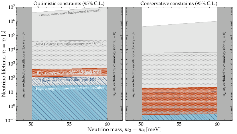
Figure A1: Comparison between one-dimensional marginalized bounds on the neutrino lifetime inferred from high-energy astrophysical neutrinos and competitive bounds from the literature. Shaded regions are disfavored at 95% C.L. The bounds are obtained assuming the invisible decay of $\nu_{2}$ and $\nu_{3}$, with a common lifetime $\tau_{2}/m_{2}=\tau_{3}/m_{3}$, while $\nu_{1}$ is stable. Left: bounds obtained under optimistic assumptions. Right: bounds obtained under conservative assumptions. The bounds from the cosmic microwave background are from Ref. [201] (see also Ref. [202]); the bounds from the next Galactic core-collapse supernova, from Ref. [31]. The lower limit on $m_{2}$ and $m_{3}$ come from the measurement of the mass-squared differences, $\Delta m_{21}^{2}\equiv m_{2}^{2}-m_{1}^{2}$ and $\Delta m_{31}^{2}\equiv m_{3}^{2}-m_{1}^{2}$, in oscillation experiments; we use their best-fit values from NuFIT 5.2 [86, 87]. The upper limit on them comes from the upper limit on the sum of the neutrino masses, $m_{1}+m_{2}+m_{3}\leq 0.12$, from cosmology [203]. In both cases, we set $m_{1}=0$ to display the widest possible mass ranges, as in Fig. 1 of Ref. [39]. See Fig. A2 for an overview of all one-dimensional bounds, and Figs. 5 and 6 for the two-dimensional bounds on $\tau_{2}/m_{2}$ and $\tau_{3}/m_{3}$, no longer assuming that they are equal. See Secs. IV and V for details.

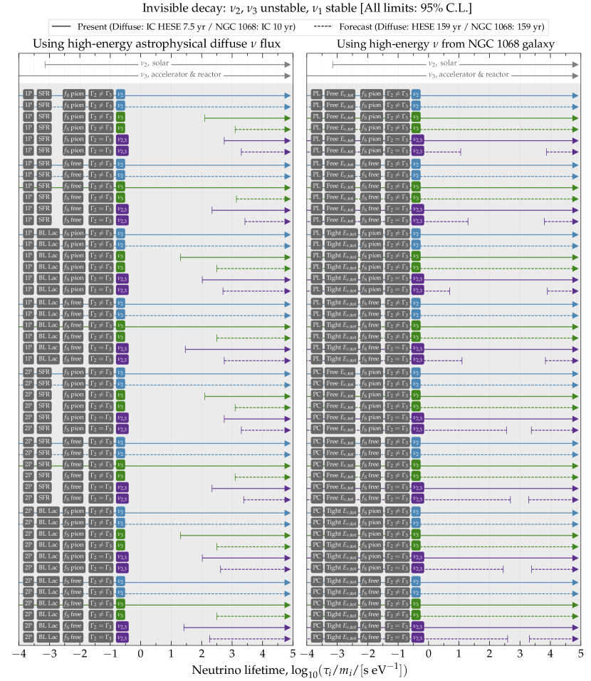
Figure A2: Overview of one-dimensional bounds on the lifetimes of $\nu_{2}$ and $\nu_{3}$. We show present-day and year-2035 one-dimensional bounds separately on $\tau_{\nu_{2}}/m_{\nu_{2}}$ and $\tau_{\nu_{3}}/m_{\nu_{3}}$, profiled over all other model parameters, for all the different scenarios that we have explored. We show bounds assuming free flavor composition at the sources (“$f_{\rm S}$ free”) or the composition from pion decay (“$f_{\rm S}$ pion”), letting $\nu_{2}$ and $\nu_{3}$ have different decay rates ($\Gamma_{2}\neq\Gamma_{3}$) or a common one ($\Gamma_{2}=\Gamma_{3}$). Left: Bounds from the diffuse high-energy neutrino flux, assuming one (1P) or two (2P) neutrino source populations that evolve with redshift following the star-formation rate (SFR) or BL Lacs. Right: Bounds from neutrinos from NGC 1068, assuming either a power-law neutrino spectrum (“PL”) or a power law with a high-energy exponential cut-off (“PC”), and either no constraint on the total emitted energy in neutrinos (“Free “$E_{\nu,{\rm tot}}$”) or constraining it to be at most 50% of the energy in x-rays (“Tight “$E_{\nu,{\rm tot}}$”).

References

- Pal and Wolfenstein [1982] P. B. Pal and L. Wolfenstein, Radiative Decays of Massive Neutrinos, Phys. Rev. D 25, 766 (1982).
- Hosotani [1981] Y. Hosotani, Majorana Masses, Photon Gas Heating and Cosmological Constraints on Neutrinos, Nucl. Phys. B 191, 411 (1981), [Erratum: Nucl. Phys. B 197, 546 (1982)].
- Nieves [1983] J. F. Nieves, Two Photon Decays of Heavy Neutrinos, Phys. Rev. D 28, 1664 (1983).
- Bahcall et al. [1972] J. N. Bahcall, N. Cabibbo, and A. Yahil, Are neutrinos stable particles?, Phys. Rev. Lett. 28, 316 (1972).
- Shrock [1974] R. Shrock, Decay in gauge theories of weak and electromagnetic interactions, Phys. Rev. D 9, 743 (1974).
- Petcov [1977] S. T. Petcov, The Processes in the Weinberg-Salam Model with Neutrino Mixing, Sov. J. Nucl. Phys. 25, 340 (1977), [Erratum: Sov. J. Nucl. Phys. 25, 698 (1977), Erratum: Yad. Fiz. 25, 1336 (1977)].
- Marciano and Sanda [1977] W. J. Marciano and A. I. Sanda, Exotic Decays of the Muon and Heavy Leptons in Gauge Theories, Phys. Lett. B 67, 303 (1977).
- Zatsepin and Smirnov [1978] G. T. Zatsepin and A. Y. Smirnov, Neutrino Decay in Gauge Theories, Yad. Fiz. 28, 1569 (1978).
- Chikashige et al. [1980] Y. Chikashige, R. N. Mohapatra, and R. D. Peccei, Spontaneously Broken Lepton Number and Cosmological Constraints on the Neutrino Mass Spectrum, Phys. Rev. Lett. 45, 1926 (1980).
- Gelmini and Roncadelli [1981] G. B. Gelmini and M. Roncadelli, Left-Handed Neutrino Mass Scale and Spontaneously Broken Lepton Number, Phys. Lett. B 99, 411 (1981).
- Schechter and Valle [1982] J. Schechter and J. W. F. Valle, Neutrino Decay and Spontaneous Violation of Lepton Number, Phys. Rev. D 25, 774 (1982).
- Shrock [1982] R. E. Shrock, Electromagnetic Properties and Decays of Dirac and Majorana Neutrinos in a General Class of Gauge Theories, Nucl. Phys. B 206, 359 (1982).
- Gelmini and Valle [1984] G. B. Gelmini and J. W. F. Valle, Fast Invisible Neutrino Decays, Phys. Lett. B 142, 181 (1984).
- Bahcall et al. [1986] J. N. Bahcall, S. T. Petcov, S. Toshev, and J. W. F. Valle, Tests of Neutrino Stability, Phys. Lett. B 181, 369 (1986).
- Nussinov [1987] S. Nussinov, Some Comments on Decaying Neutrinos and the Triplet Majoron Model, Phys. Lett. B 185, 171 (1987).
- Frieman et al. [1988] J. A. Frieman, H. E. Haber, and K. Freese, Neutrino Mixing, Decays and Supernova 1987A, Phys. Lett. B 200, 115 (1988).
- Kim and Lam [1990] C. W. Kim and W. P. Lam, Some remarks on neutrino decay via a Nambu-Goldstone boson, Mod. Phys. Lett. A 5, 297 (1990).
- Pompa and Mena [2024] F. Pompa and O. Mena, How long do neutrinos live and how much do they weigh?, Eur. Phys. J. C 84, 134 (2024), arXiv:2310.05474 [hep-ph] .
- Hosaka et al. [2006] J. Hosaka et al. (Super-Kamiokande), Three flavor neutrino oscillation analysis of atmospheric neutrinos in Super-Kamiokande, Phys. Rev. D 74, 032002 (2006), arXiv:hep-ex/0604011 .
- Michael et al. [2006] D. G. Michael et al. (MINOS), Observation of muon neutrino disappearance with the MINOS detectors and the NuMI neutrino beam, Phys. Rev. Lett. 97, 191801 (2006), arXiv:hep-ex/0607088 .
- Ahn et al. [2006] M. H. Ahn et al. (K2K), Measurement of Neutrino Oscillation by the K2K Experiment, Phys. Rev. D 74, 072003 (2006), arXiv:hep-ex/0606032 .
- González-García and Maltoni [2008] M. C. González-García and M. Maltoni, Status of Oscillation plus Decay of Atmospheric and Long-Baseline Neutrinos, Phys. Lett. B 663, 405 (2008), arXiv:0802.3699 [hep-ph] .
- Gomes et al. [2015] R. A. Gomes, A. L. G. Gomes, and O. L. G. Peres, Constraints on neutrino decay lifetime using long-baseline charged and neutral current data, Phys. Lett. B 740, 345 (2015), arXiv:1407.5640 [hep-ph] .
- Abrahão et al. [2015] T. Abrahão, H. Minakata, H. Nunokawa, and A. A. Quiroga, Constraint on Neutrino Decay with Medium-Baseline Reactor Neutrino Oscillation Experiments, JHEP 11, 001, arXiv:1506.02314 [hep-ph] .
- Choubey et al. [2018a] S. Choubey, S. Goswami, and D. Pramanik, A study of invisible neutrino decay at DUNE and its effects on measurement, JHEP 02, 055, arXiv:1705.05820 [hep-ph] .
- Choubey et al. [2018b] S. Choubey, D. Dutta, and D. Pramanik, Invisible neutrino decay in the light of NOvA and T2K data, JHEP 08, 141, arXiv:1805.01848 [hep-ph] .
- de Salas et al. [2019] P. F. de Salas, S. Pastor, C. A. Ternes, T. Thakore, and M. Tórtola, Constraining the invisible neutrino decay with KM3NeT-ORCA, Phys. Lett. B 789, 472 (2019), arXiv:1810.10916 [hep-ph] .
- Abdullahi and Denton [2020] A. Abdullahi and P. B. Denton, Visible Decay of Astrophysical Neutrinos at IceCube, Phys. Rev. D 102, 023018 (2020), arXiv:2005.07200 [hep-ph] .
- Ackermann et al. [2022] M. Ackermann et al., High-energy and ultra-high-energy neutrinos: A Snowmass white paper, JHEAp 36, 55 (2022), arXiv:2203.08096 [hep-ph] .
- Ternes and Pagliaroli [2024] C. A. Ternes and G. Pagliaroli, Invisible neutrino decay at long-baseline neutrino oscillation experiments, (2024), arXiv:2401.14316 [hep-ph] .
- Martínez-Miravé et al. [2024] P. Martínez-Miravé, I. Tamborra, and M. Tórtola, The Sun and core-collapse supernovae are leading probes of the neutrino lifetime, JCAP 05, 002, arXiv:2402.00116 [astro-ph.HE] .
- Beacom and Bell [2002] J. F. Beacom and N. F. Bell, Do Solar Neutrinos Decay?, Phys. Rev. D 65, 113009 (2002), arXiv:hep-ph/0204111 .
- Berryman et al. [2015] J. M. Berryman, A. de Gouvêa, and D. Hernández, Solar Neutrinos and the Decaying Neutrino Hypothesis, Phys. Rev. D 92, 073003 (2015), arXiv:1411.0308 [hep-ph] .
- Hirata et al. [1987] K. Hirata et al. (Kamiokande-II), Observation of a Neutrino Burst from the Supernova SN 1987a, Phys. Rev. Lett. 58, 1490 (1987).
- Bionta et al. [1987] R. M. Bionta et al., Observation of a Neutrino Burst in Coincidence with Supernova SN 1987a in the Large Magellanic Cloud, Phys. Rev. Lett. 58, 1494 (1987).
- Alekseev et al. [1988] E. N. Alekseev, L. N. Alekseeva, I. V. Krivosheina, and V. I. Volchenko, Detection of the Neutrino Signal From SN1987A in the LMC Using the Inr Baksan Underground Scintillation Telescope, Phys. Lett. B 205, 209 (1988).
- Iváñez Ballesteros and Volpe [2023] P. Iváñez Ballesteros and M. C. Volpe, SN1987A and neutrino non-radiative decay, Phys. Lett. B 847, 138252 (2023), arXiv:2307.03549 [hep-ph] .
- Aartsen et al. [2013] M. G. Aartsen et al. (IceCube), Evidence for High-Energy Extraterrestrial Neutrinos at the IceCube Detector, Science 342, 1242856 (2013), arXiv:1311.5238 [astro-ph.HE] .
- Bustamante et al. [2017] M. Bustamante, J. F. Beacom, and K. Murase, Testing decay of astrophysical neutrinos with incomplete information, Phys. Rev. D 95, 063013 (2017), arXiv:1610.02096 [astro-ph.HE] .
- Shoemaker and Murase [2016] I. M. Shoemaker and K. Murase, Probing BSM Neutrino Physics with Flavor and Spectral Distortions: Prospects for Future High-Energy Neutrino Telescopes, Phys. Rev. D 93, 085004 (2016), arXiv:1512.07228 [astro-ph.HE] .
- Denton and Tamborra [2018] P. B. Denton and I. Tamborra, Invisible Neutrino Decay Could Resolve IceCube’s Track and Cascade Tension, Phys. Rev. Lett. 121, 121802 (2018), arXiv:1805.05950 [hep-ph] .
- Abbasi et al. [2022a] R. Abbasi et al. (IceCube), Evidence for neutrino emission from the nearby active galaxy NGC 1068, Science 378, 538 (2022a).
- IceCube Collaboration [2021] IceCube Collaboration, HESE 7.5 year data release, https://icecube.wisc.edu/data-releases/2021/12/hese-7-5-year-data/ (2021).
- Schumacher et al. [2024] L. J. Schumacher, M. Huber, and M. Bustamante, PLEM, https://github.com/PLEnuM-group/Plenum (2024).
- Pakvasa [1981] S. Pakvasa, Charged lepton oscillations, Lett. Nuovo Cim. 31, 497 (1981).
- Beacom et al. [2003a] J. F. Beacom, N. F. Bell, D. Hooper, S. Pakvasa, and T. J. Weiler, Decay of High-Energy Astrophysical Neutrinos, Phys. Rev. Lett. 90, 181301 (2003a), arXiv:hep-ph/0211305 .
- Barenboim and Quigg [2003] G. Barenboim and C. Quigg, Neutrino observatories can characterize cosmic sources and neutrino properties, Phys. Rev. D 67, 073024 (2003), arXiv:hep-ph/0301220 .
- Beacom et al. [2003b] J. F. Beacom, N. F. Bell, D. Hooper, S. Pakvasa, and T. J. Weiler, Measuring flavor ratios of high-energy astrophysical neutrinos, Phys. Rev. D 68, 093005 (2003b), [Erratum: Phys. Rev. D 72, 019901 (2005)], arXiv:hep-ph/0307025 .
- Beacom et al. [2004a] J. F. Beacom, N. F. Bell, D. Hooper, S. Pakvasa, and T. J. Weiler, Sensitivity to and in the decaying astrophysical neutrino scenario, Phys. Rev. D 69, 017303 (2004a), arXiv:hep-ph/0309267 .
- Meloni and Ohlsson [2007] D. Meloni and T. Ohlsson, Neutrino flux ratios at neutrino telescopes: The role of uncertainties of neutrino mixing parameters and applications to neutrino decay, Phys. Rev. D 75, 125017 (2007), arXiv:hep-ph/0612279 .
- Maltoni and Winter [2008] M. Maltoni and W. Winter, Testing neutrino oscillations plus decay with neutrino telescopes, JHEP 07, 064, arXiv:0803.2050 [hep-ph] .
- Bustamante et al. [2010] M. Bustamante, A. M. Gago, and C. Peña-Garay, Energy-Independent New Physics in the Flavour Ratios of High-Energy Astrophysical Neutrinos, JHEP 04, 066, arXiv:1001.4878 [hep-ph] .
- Baerwald et al. [2012a] P. Baerwald, M. Bustamante, and W. Winter, Neutrino Decays over Cosmological Distances and the Implications for Neutrino Telescopes, JCAP 10, 020, arXiv:1208.4600 [astro-ph.CO] .
- Pakvasa et al. [2013] S. Pakvasa, A. Joshipura, and S. Mohanty, Explanation for the low flux of high energy astrophysical muon-neutrinos, Phys. Rev. Lett. 110, 171802 (2013), arXiv:1209.5630 [hep-ph] .
- Dorame et al. [2013] L. Dorame, O. G. Miranda, and J. W. F. Valle, Invisible decays of ultra-high energy neutrinos, Front. in Phys. 1, 25 (2013), arXiv:1303.4891 [hep-ph] .
- Pagliaroli et al. [2015] G. Pagliaroli, A. Palladino, F. L. Villante, and F. Vissani, Testing nonradiative neutrino decay scenarios with IceCube data, Phys. Rev. D 92, 113008 (2015), arXiv:1506.02624 [hep-ph] .
- Bustamante et al. [2015] M. Bustamante, J. F. Beacom, and W. Winter, Theoretically palatable flavor combinations of astrophysical neutrinos, Phys. Rev. Lett. 115, 161302 (2015), arXiv:1506.02645 [astro-ph.HE] .
- Huang and Ma [2015] Y. Huang and B.-Q. Ma, Neutrino properties from ultra-high energy cosmic neutrinos, The Universe 3, 15 (2015), arXiv:1508.01698 [hep-ph] .
- Aartsen et al. [2018a] M. G. Aartsen et al. (IceCube), Neutrino emission from the direction of the blazar TXS 0506+056 prior to the IceCube-170922A alert, Science 361, 147 (2018a), arXiv:1807.08794 [astro-ph.HE] .
- Aartsen et al. [2018b] M. G. Aartsen et al. (IceCube, Fermi-LAT, MAGIC, AGILE, ASAS-SN, HAWC, H.E.S.S., INTEGRAL, Kanata, Kiso, Kapteyn, Liverpool Telescope, Subaru, Swift NuSTAR, VERITAS, VLA/17B-403), Multimessenger observations of a flaring blazar coincident with high-energy neutrino IceCube-170922A, Science 361, eaat1378 (2018b), arXiv:1807.08816 [astro-ph.HE] .
- Stein et al. [2021] R. Stein et al., A tidal disruption event coincident with a high-energy neutrino, Nature Astron. 5, 510 (2021), arXiv:2005.05340 [astro-ph.HE] .
- Reusch et al. [2022] S. Reusch et al., Candidate Tidal Disruption Event AT2019fdr Coincident with a High-Energy Neutrino, Phys. Rev. Lett. 128, 221101 (2022), arXiv:2111.09390 [astro-ph.HE] .
- Valera et al. [2023] V. B. Valera, D. Fiorillo, I. Esteban, and M. Bustamante, Probing Neutrino Decay Using the First Steady-State Source of High-Energy Astrophysical Neutrinos, NGC 1068, PoS ICRC2023, 1066 (2023).
- Aynutdinov et al. [2023] V. M. Aynutdinov et al. (Baikal-GVD), Large neutrino telescope Baikal-GVD: recent status, PoS ICRC2023, 976 (2023), arXiv:2309.16310 [astro-ph.HE] .
- Aartsen et al. [2021] M. G. Aartsen et al. (IceCube-Gen2), IceCube-Gen2: the window to the extreme Universe, J. Phys. G 48, 060501 (2021), arXiv:2008.04323 [astro-ph.HE] .
- Adrián-Martínez et al. [2016] S. Adrián-Martínez et al. (KM3Net), Letter of intent for KM3NeT 2.0, J. Phys. G 43, 084001 (2016), arXiv:1601.07459 [astro-ph.IM] .
- Agostini et al. [2020] M. Agostini et al. (P-ONE), The Pacific Ocean Neutrino Experiment, Nature Astron. 4, 913 (2020), arXiv:2005.09493 [astro-ph.HE] .
- Thompson [2023] W. G. Thompson (TAMBO), TAMBO: Searching for Tau Neutrinos in the Peruvian Andes, in 38th International Cosmic Ray Conference (2023) arXiv:2308.09753 [astro-ph.HE] .
- Ye et al. [2022] Z. P. Ye et al., Proposal for a neutrino telescope in South China Sea, (2022), arXiv:2207.04519 [astro-ph.HE] .
- Pontecorvo [1957] B. Pontecorvo, Inverse beta processes and nonconservation of lepton charge, Zh. Eksp. Teor. Fiz. 34, 247 (1957).
- Maki et al. [1962] Z. Maki, M. Nakagawa, and S. Sakata, Remarks on the unified model of elementary particles, Prog. Theor. Phys. 28, 870 (1962).
- Mehta and Winter [2011] P. Mehta and W. Winter, Interplay of energy dependent astrophysical neutrino flavor ratios and new physics effects, JCAP 03, 041, arXiv:1101.2673 [hep-ph] .
- Fiorillo et al. [2023] D. F. G. Fiorillo, M. Heinlein, H.-T. Janka, G. Raffelt, E. Vitagliano, and R. Bollig, Supernova simulations confront SN 1987A neutrinos, Phys. Rev. D 108, 083040 (2023), arXiv:2308.01403 [astro-ph.HE] .
- Mücke et al. [2000] A. Mücke, R. Engel, J. P. Rachen, R. J. Protheroe, and T. Stanev, SOPHIA: Monte Carlo simulations of photohadronic processes in astrophysics, Comput. Phys. Commun. 124, 290 (2000), arXiv:astro-ph/9903478 .
- Kashti and Waxman [2005] T. Kashti and E. Waxman, Flavoring astrophysical neutrinos: Flavor ratios depend on energy, Phys. Rev. Lett. 95, 181101 (2005), arXiv:astro-ph/0507599 .
- Lipari et al. [2007] P. Lipari, M. Lusignoli, and D. Meloni, Flavor Composition and Energy Spectrum of Astrophysical Neutrinos, Phys. Rev. D 75, 123005 (2007), arXiv:0704.0718 [astro-ph] .
- Hümmer et al. [2010a] S. Hümmer, M. Maltoni, W. Winter, and C. Yaguna, Energy dependent neutrino flavor ratios from cosmic accelerators on the Hillas plot, Astropart. Phys. 34, 205 (2010a), arXiv:1007.0006 [astro-ph.HE] .
- Hümmer et al. [2010b] S. Hümmer, M. Rüger, F. Spanier, and W. Winter, Simplified models for photohadronic interactions in cosmic accelerators, Astrophys. J. 721, 630 (2010b), arXiv:1002.1310 [astro-ph.HE] .
- Baerwald et al. [2011] P. Baerwald, S. Hümmer, and W. Winter, Magnetic Field and Flavor Effects on the Gamma-Ray Burst Neutrino Flux, Phys. Rev. D 83, 067303 (2011), arXiv:1009.4010 [astro-ph.HE] .
- Baerwald et al. [2012b] P. Baerwald, S. Hümmer, and W. Winter, Systematics in the Interpretation of Aggregated Neutrino Flux Limits and Flavor Ratios from Gamma-Ray Bursts, Astropart. Phys. 35, 508 (2012b), arXiv:1107.5583 [astro-ph.HE] .
- Winter [2012] W. Winter, Neutrinos from Cosmic Accelerators Including Magnetic Field and Flavor Effects, Adv. High Energy Phys. 2012, 586413 (2012), arXiv:1201.5462 [astro-ph.HE] .
- Roulet and Vissani [2021] E. Roulet and F. Vissani, On the energy of the protons producing the very high-energy astrophysical neutrinos, JCAP 03, 050, arXiv:2011.12769 [astro-ph.HE] .
- Fiorillo et al. [2021a] D. F. G. Fiorillo, A. Van Vliet, S. Morisi, and W. Winter, Unified thermal model for photohadronic neutrino production in astrophysical sources, JCAP 07, 028, arXiv:2103.16577 [astro-ph.HE] .
- Farzan and Smirnov [2008] Y. Farzan and A. Y. Smirnov, Coherence and oscillations of cosmic neutrinos, Nucl. Phys. B 805, 356 (2008), arXiv:0803.0495 [hep-ph] .
- Fiorillo [2024] D. F. G. Fiorillo, High-Energy and Ultra-High-Energy Neutrino Astrophysics, Universe 10, 149 (2024).
- Esteban et al. [2020] I. Esteban, M. C. González-García, M. Maltoni, T. Schwetz, and A. Zhou, The fate of hints: updated global analysis of three-flavor neutrino oscillations, JHEP 09, 178, arXiv:2007.14792 [hep-ph] .
- Esteban et al. [2022] I. Esteban, M. C. González-García, M. Maltoni, T. Schwetz, and A. Zhou, http://www.nu-fit.org/ (2022), NuFIT 5.2.
- Argüelles et al. [2015] C. A. Argüelles, T. Katori, and J. Salvadó, New Physics in Astrophysical Neutrino Flavor, Phys. Rev. Lett. 115, 161303 (2015), arXiv:1506.02043 [hep-ph] .
- Song et al. [2021] N. Song, S. W. Li, C. A. Argüelles, M. Bustamante, and A. C. Vincent, The Future of High-Energy Astrophysical Neutrino Flavor Measurements, JCAP 04, 054, arXiv:2012.12893 [hep-ph] .
- Liu et al. [2023] Q. Liu, D. F. G. Fiorillo, C. A. Argüelles, M. Bustamante, N. Song, and A. C. Vincent, Identifying Energy-Dependent Flavor Transitions in High-Energy Astrophysical Neutrino Measurements, (2023), arXiv:2312.07649 [astro-ph.HE] .
- Rasmussen et al. [2017] R. W. Rasmussen, L. Lechner, M. Ackermann, M. Kowalski, and W. Winter, Astrophysical neutrinos flavored with Beyond the Standard Model physics, Phys. Rev. D 96, 083018 (2017), arXiv:1707.07684 [hep-ph] .
- Abbasi et al. [2022b] R. Abbasi et al. (IceCube), Detection of astrophysical tau neutrino candidates in IceCube, Eur. Phys. J. C 82, 1031 (2022b), arXiv:2011.03561 [hep-ex] .
- Rachen and Meszaros [1998] J. P. Rachen and P. Meszaros, Photohadronic neutrinos from transients in astrophysical sources, Phys. Rev. D 58, 123005 (1998), arXiv:astro-ph/9802280 .
- Athar et al. [2000] H. Athar, M. Jezabek, and O. Yasuda, Effects of neutrino mixing on high-energy cosmic neutrino flux, Phys. Rev. D 62, 103007 (2000), arXiv:hep-ph/0005104 .
- Crocker et al. [2002] R. M. Crocker, F. Melia, and R. R. Volkas, Searching for long wavelength neutrino oscillations in the distorted neutrino spectrum of galactic supernova remnants, Astrophys. J. Suppl. 141, 147 (2002), arXiv:astro-ph/0106090 .
- Beacom and Candia [2004] J. F. Beacom and J. Candia, Shower power: Isolating the prompt atmospheric neutrino flux using electron neutrinos, JCAP 11, 009, arXiv:hep-ph/0409046 .
- Mena et al. [2007] O. Mena, I. Mocioiu, and S. Razzaque, Oscillation effects on high-energy neutrino fluxes from astrophysical hidden sources, Phys. Rev. D 75, 063003 (2007), arXiv:astro-ph/0612325 .
- Kachelrieß and Tomàs [2006] M. Kachelrieß and R. Tomàs, High energy neutrino yields from astrophysical sources I: Weakly magnetized sources, Phys. Rev. D 74, 063009 (2006), arXiv:astro-ph/0606406 .
- Esmaili and Farzan [2009] A. Esmaili and Y. Farzan, An Analysis of Cosmic Neutrinos: Flavor Composition at Source and Neutrino Mixing Parameters, Nucl. Phys. B 821, 197 (2009), arXiv:0905.0259 [hep-ph] .
- Choubey and Rodejohann [2009] S. Choubey and W. Rodejohann, Flavor Composition of UHE Neutrinos at Source and at Neutrino Telescopes, Phys. Rev. D 80, 113006 (2009), arXiv:0909.1219 [hep-ph] .
- Bustamante et al. [2011] M. Bustamante, A. M. Gago, and J. Jones Pérez, SUSY Renormalization Group Effects in Ultra High Energy Neutrinos, JHEP 05, 133, arXiv:1012.2728 [hep-ph] .
- Winter [2013] W. Winter, Photohadronic Origin of the TeV-PeV Neutrinos Observed in IceCube, Phys. Rev. D 88, 083007 (2013), arXiv:1307.2793 [astro-ph.HE] .
- Palladino et al. [2015] A. Palladino, G. Pagliaroli, F. L. Villante, and F. Vissani, What is the Flavor of the Cosmic Neutrinos Seen by IceCube?, Phys. Rev. Lett. 114, 171101 (2015), arXiv:1502.02923 [astro-ph.HE] .
- Biehl et al. [2017] D. Biehl, A. Fedynitch, A. Palladino, T. J. Weiler, and W. Winter, Astrophysical Neutrino Production Diagnostics with the Glashow Resonance, JCAP 01, 033, arXiv:1611.07983 [astro-ph.HE] .
- Bustamante and Ahlers [2019] M. Bustamante and M. Ahlers, Inferring the flavor of high-energy astrophysical neutrinos at their sources, Phys. Rev. Lett. 122, 241101 (2019), arXiv:1901.10087 [astro-ph.HE] .
- Ackermann et al. [2019a] M. Ackermann et al., Astrophysics Uniquely Enabled by Observations of High-Energy Cosmic Neutrinos, Bull. Am. Astron. Soc. 51, 185 (2019a), arXiv:1903.04334 [astro-ph.HE] .
- Bustamante and Tamborra [2020] M. Bustamante and I. Tamborra, Using high-energy neutrinos as cosmic magnetometers, Phys. Rev. D 102, 123008 (2020), arXiv:2009.01306 [astro-ph.HE] .
- Bhattacharya et al. [2023] A. Bhattacharya, R. Enberg, M. H. Reno, and I. Sarcevic, Energy-dependent flavour ratios in neutrino telescopes from charm, (2023), arXiv:2309.09139 [astro-ph.HE] .
- Telalovic and Bustamante [2023] B. Telalovic and M. Bustamante, Flavor Anisotropy in the High-Energy Astrophysical Neutrino Sky, (2023), arXiv:2310.15224 [astro-ph.HE] .
- Dev et al. [2023] P. S. B. Dev, S. Jana, and Y. Porto, Flavor Matters, but Matter Flavors: Matter Effects on Flavor Composition of Astrophysical Neutrinos, (2023), arXiv:2312.17315 [hep-ph] .
- Capanema et al. [2024] A. Capanema, Y. Porto, and M. M. Saez, The Flavor Composition of Supernova Neutrinos, (2024), arXiv:2403.14762 [hep-ph] .
- Beacom et al. [2004b] J. F. Beacom, N. F. Bell, D. Hooper, J. G. Learned, S. Pakvasa, and T. J. Weiler, PseudoDirac neutrinos: A Challenge for neutrino telescopes, Phys. Rev. Lett. 92, 011101 (2004b), arXiv:hep-ph/0307151 .
- Serpico [2006] P. D. Serpico, Probing the 2-3 leptonic mixing at high-energy neutrino telescopes, Phys. Rev. D 73, 047301 (2006), arXiv:hep-ph/0511313 .
- Pakvasa et al. [2008] S. Pakvasa, W. Rodejohann, and T. J. Weiler, Flavor Ratios of Astrophysical Neutrinos: Implications for Precision Measurements, JHEP 02, 005, arXiv:0711.4517 [hep-ph] .
- Esmaili [2010] A. Esmaili, Pseudo-Dirac Neutrino Scenario: Cosmic Neutrinos at Neutrino Telescopes, Phys. Rev. D 81, 013006 (2010), arXiv:0909.5410 [hep-ph] .
- Bhattacharya et al. [2010a] A. Bhattacharya, S. Choubey, R. Gandhi, and A. Watanabe, Diffuse Ultra-High Energy Neutrino Fluxes and Physics Beyond the Standard Model, Phys. Lett. B 690, 42 (2010a), arXiv:0910.4396 [hep-ph] .
- Bhattacharya et al. [2010b] A. Bhattacharya, S. Choubey, R. Gandhi, and A. Watanabe, Ultra-high neutrino fluxes as a probe for non-standard physics, JCAP 09, 009, arXiv:1006.3082 [hep-ph] .
- Fu et al. [2012] L. Fu, C. M. Ho, and T. J. Weiler, Cosmic Neutrino Flavor Ratios with Broken - Symmetry, Phys. Lett. B 718, 558 (2012), arXiv:1209.5382 [hep-ph] .
- Chatterjee et al. [2014] A. Chatterjee, M. M. Devi, M. Ghosh, R. Moharana, and S. K. Raut, Probing CP violation with the first three years of ultrahigh energy neutrinos from IceCube, Phys. Rev. D 90, 073003 (2014), arXiv:1312.6593 [hep-ph] .
- Xu et al. [2014] X.-J. Xu, H.-J. He, and W. Rodejohann, Constraining Astrophysical Neutrino Flavor Composition from Leptonic Unitarity, JCAP 12, 039, arXiv:1407.3736 [hep-ph] .
- Aeikens et al. [2015] E. Aeikens, H. Päs, S. Pakvasa, and P. Sicking, Flavor ratios of extragalactic neutrinos and neutrino shortcuts in extra dimensions, JCAP 10, 005, arXiv:1410.0408 [hep-ph] .
- de Salas et al. [2016] P. F. de Salas, R. A. Lineros, and M. Tórtola, Neutrino propagation in the galactic dark matter halo, Phys. Rev. D 94, 123001 (2016), arXiv:1601.05798 [astro-ph.HE] .
- González-García et al. [2016] M. C. González-García, M. Maltoni, I. Martínez-Soler, and N. Song, Non-standard neutrino interactions in the Earth and the flavor of astrophysical neutrinos, Astropart. Phys. 84, 15 (2016), arXiv:1605.08055 [hep-ph] .
- Dey et al. [2018] U. K. Dey, D. Kar, M. Mitra, M. Spannowsky, and A. C. Vincent, Searching for Leptoquarks at IceCube and the LHC, Phys. Rev. D 98, 035014 (2018), arXiv:1709.02009 [hep-ph] .
- Bustamante and Agarwalla [2019] M. Bustamante and S. K. Agarwalla, Universe’s Worth of Electrons to Probe Long-Range Interactions of High-Energy Astrophysical Neutrinos, Phys. Rev. Lett. 122, 061103 (2019), arXiv:1808.02042 [astro-ph.HE] .
- Farzan and Palomares-Ruiz [2019] Y. Farzan and S. Palomares-Ruiz, Flavor of cosmic neutrinos preserved by ultralight dark matter, Phys. Rev. D 99, 051702 (2019), arXiv:1810.00892 [hep-ph] .
- Ahlers et al. [2018] M. Ahlers, M. Bustamante, and S. Mu, Unitarity Bounds of Astrophysical Neutrinos, Phys. Rev. D 98, 123023 (2018), arXiv:1810.00893 [astro-ph.HE] .
- Brdar and Hansen [2019] V. Brdar and R. S. L. Hansen, IceCube Flavor Ratios with Identified Astrophysical Sources: Towards Improving New Physics Testability, JCAP 02, 023, arXiv:1812.05541 [hep-ph] .
- Palladino [2019] A. Palladino, The flavor composition of astrophysical neutrinos after 8 years of IceCube: an indication of neutron decay scenario?, Eur. Phys. J. C 79, 500 (2019), arXiv:1902.08630 [astro-ph.HE] .
- Ackermann et al. [2019b] M. Ackermann et al., Fundamental Physics with High-Energy Cosmic Neutrinos, Bull. Am. Astron. Soc. 51, 215 (2019b), arXiv:1903.04333 [astro-ph.HE] .
- Argüelles et al. [2020] C. A. Argüelles, M. Bustamante, A. Kheirandish, S. Palomares-Ruiz, J. Salvadó, and A. C. Vincent, Fundamental physics with high-energy cosmic neutrinos today and in the future, PoS ICRC2019, 849 (2020), arXiv:1907.08690 [astro-ph.HE] .
- Ahlers et al. [2021] M. Ahlers, M. Bustamante, and N. G. N. Willesen, Flavors of astrophysical neutrinos with active-sterile mixing, JCAP 07, 029, arXiv:2009.01253 [hep-ph] .
- Karmakar et al. [2021] S. Karmakar, S. Pandey, and S. Rakshit, Astronomy with energy dependent flavour ratios of extragalactic neutrinos, JHEP 10, 004, arXiv:2010.07336 [hep-ph] .
- Fiorillo et al. [2021b] D. F. G. Fiorillo, G. Mangano, S. Morisi, and O. Pisanti, IceCube constraints on violation of equivalence principle, JCAP 04, 079, arXiv:2012.07867 [hep-ph] .
- Argüelles et al. [2023] C. A. Argüelles et al., Snowmass white paper: beyond the standard model effects on neutrino flavor: Submitted to the proceedings of the US community study on the future of particle physics (Snowmass 2021), Eur. Phys. J. C 83, 15 (2023), arXiv:2203.10811 [hep-ph] .
- Mammen Abraham et al. [2022] R. Mammen Abraham et al., Tau neutrinos in the next decade: from GeV to EeV, J. Phys. G 49, 110501 (2022), arXiv:2203.05591 [hep-ph] .
- Mena et al. [2014] O. Mena, S. Palomares-Ruiz, and A. C. Vincent, Flavor Composition of the High-Energy Neutrino Events in IceCube, Phys. Rev. Lett. 113, 091103 (2014), arXiv:1404.0017 [astro-ph.HE] .
- Palomares-Ruiz et al. [2015] S. Palomares-Ruiz, A. C. Vincent, and O. Mena, Spectral analysis of the high-energy IceCube neutrinos, Phys. Rev. D 91, 103008 (2015), arXiv:1502.02649 [astro-ph.HE] .
- Aartsen et al. [2015a] M. G. Aartsen et al. (IceCube), Flavor Ratio of Astrophysical Neutrinos above 35 TeV in IceCube, Phys. Rev. Lett. 114, 171102 (2015a), arXiv:1502.03376 [astro-ph.HE] .
- Palladino and Vissani [2015] A. Palladino and F. Vissani, The natural parameterization of cosmic neutrino oscillations, Eur. Phys. J. C 75, 433 (2015), arXiv:1504.05238 [hep-ph] .
- Aartsen et al. [2015b] M. G. Aartsen et al. (IceCube), A combined maximum-likelihood analysis of the high-energy astrophysical neutrino flux measured with IceCube, Astrophys. J. 809, 98 (2015b), arXiv:1507.03991 [astro-ph.HE] .
- Vincent et al. [2016] A. C. Vincent, S. Palomares-Ruiz, and O. Mena, Analysis of the 4-year IceCube high-energy starting events, Phys. Rev. D 94, 023009 (2016), arXiv:1605.01556 [astro-ph.HE] .
- Abbasi et al. [2021] R. Abbasi et al. (IceCube), The IceCube high-energy starting event sample: Description and flux characterization with 7.5 years of data, Phys. Rev. D 104, 022002 (2021), arXiv:2011.03545 [astro-ph.HE] .
- Workman et al. [2022] R. L. Workman et al. (Particle Data Group), Review of Particle Physics, PTEP 2022, 083C01 (2022).
- Hopkins and Beacom [2006] A. M. Hopkins and J. F. Beacom, On the Normalization of the Cosmic Star Formation History, Astrophys. J. 651, 142 (2006), arXiv:astro-ph/0601463 [astro-ph] .
- Aartsen et al. [2020] M. G. Aartsen et al. (IceCube), Time-Integrated Neutrino Source Searches with 10 Years of IceCube Data, Phys. Rev. Lett. 124, 051103 (2020), arXiv:1910.08488 [astro-ph.HE] .
- Acciari et al. [2019] V. A. Acciari et al. (MAGIC), Constraints on gamma-ray and neutrino emission from NGC 1068 with the MAGIC telescopes, Astrophys. J. 883, 135 (2019), arXiv:1906.10954 [astro-ph.HE] .
- Lenain et al. [2010] J.-P. Lenain, C. Ricci, M. Turler, D. Dorner, and R. Walter, Seyfert 2 galaxies in the GeV band: jets and starburst, Astron. Astrophys. 524, A72 (2010), arXiv:1008.5164 [astro-ph.CO] .
- Yoast-Hull et al. [2014] T. M. Yoast-Hull, J. S. G. III, E. G. Zweibel, and J. E. Everett, Active Galactic Nuclei, Neutrinos, and Interacting Cosmic Rays in NGC 253 and NGC 1068, Astrophys. J. 780, 137 (2014), arXiv:1311.5586 [astro-ph.HE] .
- Ambrosone et al. [2021] A. Ambrosone, M. Chianese, D. F. G. Fiorillo, A. Marinelli, and G. Miele, Could Nearby Star-forming Galaxies Light Up the Pointlike Neutrino Sky?, Astrophys. J. Lett. 919, L32 (2021), arXiv:2106.13248 [astro-ph.HE] .
- Eichmann et al. [2022] B. Eichmann, F. Oikonomou, S. Salvatore, R.-J. Dettmar, and J. Becker Tjus, Solving the Multimessenger Puzzle of the AGN-starburst Composite Galaxy NGC 1068, Astrophys. J. 939, 43 (2022), arXiv:2207.00102 [astro-ph.HE] .
- Lamastra et al. [2016] A. Lamastra, F. Fiore, D. Guetta, L. A. Antonelli, S. Colafrancesco, N. Menci, S. Puccetti, A. Stamerra, and L. Zappacosta, Galactic outflow driven by the active nucleus and the origin of the gamma-ray emission in NGC 1068, Astron. Astrophys. 596, A68 (2016), arXiv:1609.09664 [astro-ph.HE] .
- Peretti et al. [2023] E. Peretti, A. Lamastra, F. G. Saturni, M. Ahlers, P. Blasi, G. Morlino, and P. Cristofari, Diffusive shock acceleration at EeV and associated multimessenger flux from ultra-fast outflows driven by active galactic nuclei, Mon. Not. Roy. Astron. Soc. 526, 181 (2023), arXiv:2301.13689 [astro-ph.HE] .
- Murase [2022] K. Murase, Hidden Hearts of Neutrino Active Galaxies, Astrophys. J. Lett. 941, L17 (2022), arXiv:2211.04460 [astro-ph.HE] .
- Inoue et al. [2020] Y. Inoue, D. Khangulyan, and A. Doi, On the Origin of High-energy Neutrinos from NGC 1068: The Role of Nonthermal Coronal Activity, Astrophys. J. Lett. 891, L33 (2020), arXiv:1909.02239 [astro-ph.HE] .
- Murase et al. [2020] K. Murase, S. S. Kimura, and P. Mészáros, Hidden Cores of Active Galactic Nuclei as the Origin of Medium-Energy Neutrinos: Critical Tests with the MeV Gamma-Ray Connection, Phys. Rev. Lett. 125, 011101 (2020), arXiv:1904.04226 [astro-ph.HE] .
- Kheirandish et al. [2021] A. Kheirandish, K. Murase, and S. S. Kimura, High-energy Neutrinos from Magnetized Coronae of Active Galactic Nuclei and Prospects for Identification of Seyfert Galaxies and Quasars in Neutrino Telescopes, Astrophys. J. 922, 45 (2021), arXiv:2102.04475 [astro-ph.HE] .
- Mbarek et al. [2023] R. Mbarek, A. Philippov, A. Chernoglazov, A. Levinson, and R. Mushotzky, The Interplay between accelerated Protons, X-rays and Neutrinos in the Corona of NGC 1068: Constraints from Kinetic Plasma Simulations, (2023), arXiv:2310.15222 [astro-ph.HE] .
- Fiorillo et al. [2024] D. F. G. Fiorillo, M. Petropoulou, L. Comisso, E. Peretti, and L. Sironi, TeV Neutrinos and Hard X-Rays from Relativistic Reconnection in the Corona of NGC 1068, Astrophys. J. 961, L14 (2024), arXiv:2310.18254 [astro-ph.HE] .
- Fang et al. [2023] K. Fang, E. L. Rodriguez, F. Halzen, and J. S. Gallagher, High-energy Neutrinos from the Inner Circumnuclear Region of NGC 1068, Astrophys. J. 956, 8 (2023), arXiv:2307.07121 [astro-ph.HE] .
- Caputo et al. [2022] R. Caputo et al., All-sky Medium Energy Gamma-ray Observatory eXplorer mission concept, J. Astron. Telesc. Instrum. Syst. 8, 044003 (2022), arXiv:2208.04990 [astro-ph.IM] .
- De Angelis et al. [2017] A. De Angelis et al. (e-ASTROGAM), The e-ASTROGAM mission, Exper. Astron. 44, 25 (2017), arXiv:1611.02232 [astro-ph.HE] .
- Schumacher et al. [2021] L. J. Schumacher, M. Huber, M. Agostini, M. Bustamante, F. Oikonomou, and E. Resconi, PLEM: A global and distributed monitoring system of high-energy astrophysical neutrinos, PoS ICRC2021, 1185 (2021), arXiv:2107.13534 [astro-ph.IM] .
- Guépin et al. [2022] C. Guépin, K. Kotera, and F. Oikonomou, High-energy neutrino transients and the future of multi-messenger astronomy, Nature Rev. Phys. 4, 697 (2022), arXiv:2207.12205 [astro-ph.HE] .
- Gaisser [2012] T. K. Gaisser, Spectrum of cosmic-ray nucleons, kaon production, and the atmospheric muon charge ratio, Astropart. Phys. 35, 801 (2012), arXiv:1111.6675 [astro-ph.HE] .
- Wilks [1938] S. S. Wilks, The Large-Sample Distribution of the Likelihood Ratio for Testing Composite Hypotheses, Annals Math. Statist. 9, 60 (1938).
- Cowan et al. [2011] G. Cowan, K. Cranmer, E. Gross, and O. Vitells, Asymptotic formulae for likelihood-based tests of new physics, Eur. Phys. J. C 71, 1554 (2011), [Erratum: Eur. Phys. J. C 73, 2501 (2013)], arXiv:1007.1727 [physics.data-an] .
- Valera et al. [2024] V. B. Valera, D. F. G. Fiorillo, I. Esteban, and M. Bustamante, Neutrino_Decay_Data, https://github.com/damianofiorillo/Neutrino_Decay_Data (2024).
- Li et al. [2019] S. W. Li, M. Bustamante, and J. F. Beacom, Echo Technique to Distinguish Flavors of Astrophysical Neutrinos, Phys. Rev. Lett. 122, 151101 (2019), arXiv:1606.06290 [astro-ph.HE] .
- Steuer and Köpke [2018] A. Steuer and L. Köpke (IceCube), Delayed light emission to distinguish astrophysical neutrino flavors in IceCube, PoS ICRC2017, 1008 (2018).
- Farrag et al. [2023] K. Farrag et al., Distinguishing neutrinos using the neutron echo technique with next generation ice Cherenkov telescopes, PoS ICRC2023, 1211 (2023).
- Abbasi et al. [2023a] R. Abbasi et al. (IceCube), Observation of high-energy neutrinos from the Galactic plane, Science 380, adc9818 (2023a), arXiv:2307.04427 [astro-ph.HE] .
- Alves Batista et al. [2019] R. Alves Batista et al., Open Questions in Cosmic-Ray Research at Ultrahigh Energies, Front. Astron. Space Sci. 6, 23 (2019), arXiv:1903.06714 [astro-ph.HE] .
- Fiorillo and Bustamante [2023] D. F. G. Fiorillo and M. Bustamante, Bump hunting in the diffuse flux of high-energy cosmic neutrinos, Phys. Rev. D 107, 083008 (2023), arXiv:2301.00024 [astro-ph.HE] .
- Abbasi et al. [2022c] R. Abbasi et al. (IceCube), Improved Characterization of the Astrophysical Muon–neutrino Flux with 9.5 Years of IceCube Data, Astrophys. J. 928, 50 (2022c), arXiv:2111.10299 [astro-ph.HE] .
- Abbasi et al. [2024] R. Abbasi et al., Characterization of the Astrophysical Diffuse Neutrino Flux using Starting Track Events in IceCube, (2024), arXiv:2402.18026 [astro-ph.HE] .
- Naab et al. [2023] R. Naab, E. Ganster, and Z. Zhang (IceCube), Measurement of the astrophysical diffuse neutrino flux in a combined fit of IceCube’s high energy neutrino data, PoS ICRC2023, 1064 (2023).
- Bustamante [2024] M. Bustamante, The Milky Way shines in high-energy neutrinos, Nature Rev. Phys. 6, 8 (2024), arXiv:2312.08102 [astro-ph.HE] .
- Capanema et al. [2021] A. Capanema, A. Esmaili, and P. D. Serpico, Where do IceCube neutrinos come from? Hints from the diffuse gamma-ray flux, JCAP 02, 037, arXiv:2007.07911 [hep-ph] .
- Ajello et al. [2014] M. Ajello et al., The Cosmic Evolution of Fermi BL Lacertae Objects, Astrophys. J. 780, 73 (2014), arXiv:1310.0006 [astro-ph.CO] .
- Schönert et al. [2009] S. Schönert, T. K. Gaisser, E. Resconi, and O. Schulz, Vetoing atmospheric neutrinos in a high energy neutrino telescope, Phys. Rev. D 79, 043009 (2009), arXiv:0812.4308 [astro-ph] .
- Gaisser et al. [2014] T. K. Gaisser, K. Jero, A. Karle, and J. van Santen, Generalized self-veto probability for atmospheric neutrinos, Phys. Rev. D 90, 023009 (2014), arXiv:1405.0525 [astro-ph.HE] .
- Argüelles et al. [2018] C. A. Argüelles, S. Palomares-Ruiz, A. Schneider, L. Wille, and T. Yuan, Unified atmospheric neutrino passing fractions for large-scale neutrino telescopes, JCAP 07, 047, arXiv:1805.11003 [hep-ph] .
- Abbasi et al. [2023b] R. Abbasi et al. (IceCube), Updated directions of IceCube HESE events with the latest ice model using DirectFit, PoS ICRC2023, 1030 (2023b), arXiv:2307.13878 [astro-ph.HE] .
- IceCube Collaboration [2023] IceCube Collaboration, HESE 12-year data release, https://icecube.wisc.edu/data-releases/2023/07/icecube-hese-12-year-data-release/ (2023).
- Learned and Pakvasa [1995] J. G. Learned and S. Pakvasa, Detecting oscillations at PeV energies, Astropart. Phys. 3, 267 (1995), arXiv:hep-ph/9405296 .
- Aartsen et al. [2019] M. G. Aartsen et al. (IceCube), Measurements using the inelasticity distribution of multi-TeV neutrino interactions in IceCube, Phys. Rev. D 99, 032004 (2019), arXiv:1808.07629 [hep-ex] .
- Fedynitch et al. [2012] A. Fedynitch, J. Becker Tjus, and P. Desiati, Influence of hadronic interaction models and the cosmic ray spectrum on the high energy atmospheric muon and neutrino flux, Phys. Rev. D 86, 114024 (2012), arXiv:1206.6710 [astro-ph.HE] .
- D. et al. [2021] A. A. D. et al. (Baikal-GVD), Baikal-GVD: status and first results, PoS ICHEP2020, 606 (2021), arXiv:2012.03373 [astro-ph.HE] .
- Avrorin et al. [2021] A. D. Avrorin et al. (Baikal-GVD), High-Energy Neutrino Astronomy and the Baikal-GVD Neutrino Telescope, Phys. At. Nucl. 84, 513 (2021), arXiv:2011.09209 [astro-ph.HE] .
- Margiotta [2023] A. Margiotta (KM3NeT), The KM3NeT infrastructure: Status and first results, SciPost Phys. Proc. 13, 030 (2023), arXiv:2208.07370 [astro-ph.IM] .
- Romero-Wolf et al. [2020] A. Romero-Wolf et al., An Andean Deep-Valley Detector for High-Energy Tau Neutrinos, in Latin American Strategy Forum for Research Infrastructure (2020) arXiv:2002.06475 [astro-ph.IM] .
- Thompson et al. [2023] W. Thompson et al. (TAMBO), TAMBO: Searching for Tau Neutrinos in the Peruvian Andes, PoS ICRC2023, 1109 (2023).
- Lazar et al. [2023] J. Lazar, S. Meighen-Berger, C. Haack, D. Kim, S. Giner, and C. A. Argüelles, Prometheus: An Open-Source Neutrino Telescope Simulation, (2023), arXiv:2304.14526 [hep-ex] .
- Fuerst et al. [2023] P. M. Fuerst et al. (IceCube), Galactic and Extragalactic Analysis of the Astrophysical Muon Neutrino Flux with 12.3 years of IceCube Track Data, PoS ICRC2023, 1046 (2023), arXiv:2308.08233 [astro-ph.HE] .
- Huennefeld et al. [2021] M. Huennefeld et al. (IceCube), Combining Maximum-Likelihood with Deep Learning for Event Reconstruction in IceCube, PoS ICRC2021, 1065 (2021), arXiv:2107.12110 [astro-ph.HE] .
- Abbasi et al. [2022d] R. Abbasi et al. (IceCube), Graph Neural Networks for low-energy event classification & reconstruction in IceCube, JINST 17 (11), P11003, arXiv:2209.03042 [hep-ex] .
- Søgaard et al. [2023] A. Søgaard et al., GraphNeT: Graph neural networks for neutrino telescope event reconstruction, J. Open Source Softw. 8, 4971 (2023), arXiv:2210.12194 [astro-ph.IM] .
- Bukhari et al. [2023] H. Bukhari, D. Chakraborty, P. Eller, T. Ito, M. V. Shugaev, and R. Ørsøe, IceCube – Neutrinos in Deep Ice The Top 3 Solutions from the Public Kaggle Competition, (2023), arXiv:2310.15674 [astro-ph.HE] .
- Abbasi et al. [2023c] R. Abbasi et al. (IceCube), Summary of IceCube tau neutrino searches and flavor composition measurements of the diffuse astrophysical neutrino flux, PoS ICRC2023, 1122 (2023c), arXiv:2308.15213 [astro-ph.HE] .
- Barenboim et al. [2021] G. Barenboim, J. Z. Chen, S. Hannestad, I. M. Oldengott, T. Tram, and Y. Y. Y. Wong, Invisible neutrino decay in precision cosmology, JCAP 03, 087, arXiv:2011.01502 [astro-ph.CO] .
- Chen et al. [2022] J. Z. Chen, I. M. Oldengott, G. Pierobon, and Y. Y. Y. Wong, Weaker yet again: mass spectrum-consistent cosmological constraints on the neutrino lifetime, Eur. Phys. J. C 82, 640 (2022), arXiv:2203.09075 [hep-ph] .
- Aghanim et al. [2020] N. Aghanim et al. (Planck), Planck 2018 results. VI. Cosmological parameters, Astron. Astrophys. 641, A6 (2020), [Erratum: Astron. Astrophys. 652, C4 (2021)], arXiv:1807.06209 [astro-ph.CO] .