Efficient first-principles approach to Gibbs free energy with thermal expansion
Abstract
We propose a method to evaluate the Gibbs free energy from constant-volume first-principles calculations. The volume integral of the pressure is performed by determining the volume and the bulk modulus in equilibrium at finite temperatures, where the pressure and its volume derivative are evaluated utilizing first-principles calculations of the Grüneisen parameter without varying the volume. As an example, the validity of our method is demonstrated for fcc-Al by comparing with the conventional quasiharmonic approximation that is much more computationally-demanding.
I Introduction
The Gibbs free energy is one of the most critical quantities to understand thermodynamic properties of materials. The free energy is the basis not only for the discussion of the phase stability but also for nonequilibrium dynamics such as the evolution of microstructures. Countless experiments have been conducted and compiled into databases over the years, in line with the development of the CALPHAD (CALculation of PHAse Diagrams) method, owing to its importance. However, the evaluation of the free energy based on only experiments has become difficult with the increasing complexity of materials with multiple components. Therefore, there has been growing attention toward thermodynamics assessment through first-principles calculations, particularly using density functional theory (DFT), as a breakthrough to overcome this difficulty [1]. It goes without saying that even though DFT is valid only in the ground state, we can access finite temperature properties by combining statistical mechanical models with DFT.
For the first-principles assessment of the free energy, there are various method to incorporate some thermodynamic contributions: cluster expansion and variation method for mixing enthalpy and entropy [2, 3, 4, 5, 6, 7], phonon calculations for the vibrational free energy [8], spin-lattice models for the magnetic free energy. In addition, interactions between different contributions are also vital for the quantitative evaluation of the free energy [9, 10, 11]. For the accurate assessment of the free energy in a wide range of temperature, the contribution of thermal expansion is also important for the accuracy of a few meV/atom which is necessary to describe phase stabilities or phase transition temperatures.
The thermal expansion originates primarily due to lattice anharmonicity, at least in nonmagnetic materials. So far, a representative computational method to evaluate thermal expansion is the quasiharmonic approximation (QHA) [12, 13, 14, 15, 16, 16]. In QHA, equilibrium volume at finite temperature is determined by harmonic phonon calculations of structure models with different volumes. However, QHA is not applicable for high-temperature phases that exhibit lattice instability in low-temperature range due to the existence of imaginary frequencies. To recover the lattice stability at finite temperatures, it is necessary to consider the anharmonicity of phonons. There are several approaches to include anharmonicity, such as temperature-dependent effective potentials [17, 18, 19], piecewise polynomial potential partitioning [20, 21], self-consistent ab initio lattice dynamics [22], and self-consistent phonon theory [23, 24]. Unfortunately, in any approach, direct modeling of thermal expansion like QHA demands heavy computational costs since these methods require substantial resources even for a single volume. This is a crucial problem for the systematic evaluation of free energy for various compositional materials. Therefore, an efficient approach to evaluate the effects of thermal expansion has been required [25, 26, 27, 28, 29, 30, 31, 32].
In this study, we present an alternative approach that evaluates free energy changes due to thermal expansion from phonon calculations in a single volume, without involving calculations for many different volumes of supercells. Our approach is based on combinations of the pressure and bulk modulus of phonons and the Grüneisen theory [33]. From phonon calculations in a single volume, we calculate the equilibrium volume and equilibrium bulk modulus, which are parameters in the second-order Birch-Murnaghan equation of state at any temperature. Using these parameters, free energy changes due to thermal expansion is calculated by integrating pressure with respect to volume.
II Theory
Since it is easy to calculate the Helmholtz free energy where is the temperature and is the constant volume, we propose a method to obtain the Gibbs free energy from the .
II.1 Pressure integral method
Our objective is to determine the Gibbs free energy of a single phase, where and are the content of components, and the pressure, respectively. In the following discussion, we consider closed systems, therefore, we do not write the content of components from the variables explicitly. The Gibbs free energy can be written as:
| (1) |
where is the equilibrium volume as a function of temperature and pressure, as expressed as .
To calculate the integral term in Eq. (1), we use the second-order Birch-Murnaghan equation of state (EOS) [34, 35, 36] as
| (2) |
and its first derivative with respect to volume,
| (3) |
where is the bulk modulus at . Note that Eq. (3) is directly related to the bulk modulus as
| (4) |
Since the values on the left-hand side in Eqs. (2) and (3) are derived analytically as shown in Sec. II.2, we obtain the function through the determination of and from the phonon calculations at a single volume. Therefore, the change in the Helmholtz free energy due to thermal expansion is obtained by integrating the pressure from Eq. (2) with respect to volume. Hereafter we call this method as pressure integral method (PIM).
Within the Born-Oppenheimer approximation, the Helmholtz free energy of the entire system can be divided into the electronic and vibrational contributions [37]
| (5) |
where is the electronic free energy and is the vibrational free energy. The pressure can be divided into the electronic and vibrational contributions as follows:
| (6) |
Also, the first derivative of pressure with respect to volume can also be divided into the electronic and vibrational contributions. The electronic contributions to the free energy and pressure can be calculated within the usual finite-temperature density functional theory [38, 39].
II.2 Vibrational pressure and its volume derivative
In this part, we derive the vibrational pressure and its volume derivative from vibrationl free energy as follows:
| (7) | ||||
| (8) |
where is the volume dependent frequency of the th phonon with wave number , is the Boltzmann constant, is Bose-Einstein distribution function with zero chemical potential, and is Grüneisen parameter [30, 33, 8, 40] as follows:
| (9) | ||||
| (10) |
where is polarization vector and is a change in the dynamical matrix due to a volume change . See Appendix A for the details on the definitions. Also, the derivative of with respect to volume can be written as
| (11) | ||||
| (12) |
where we use the fact that is not explicitly dependent on in the second line of Eq. (II.2).
III Applications
We apply the PIM to fcc-Al which has a large coefficient of thermal expansion (CTE) as a demonstration. In the following calculation we have assumed zero pressure (), and in Eq. (1) is used the value obtained from structural optimization at the ground state. If the contribution of the term containing is minor, we can evaluate without changing the volume. To test the postulation, we redefine Eq. (II.2) as
| (13) |
where , and as follows:
| (14) | ||||
| (15) | ||||
| (16) |
III.1 Computational details
We performed first-principles calculations based on density functional theory within the projector augmented-wave method [41] as implemented in the VASP code [42, 43]. For the exchange-correlation functional, the generalized gradient approximation parameterized by Perdew, Burke, and Ernzerhof [44] were employed. We employed the DFT calculation for fcc-Al with supercell (108 atoms). The cutoff energy of 313 eV and gamma-centered 6 6 6 k-grid were used. The calculations of force constants and phonon frequencies are conducted by using ALAMODE package [45]. In the QHA calculation, we calculate the harmonic phonon dispersion by using the small displacement method. We also third-order IFCs were extracted using LASSO regression to calculate the Grüneisen parameter.
III.2 fcc-Al
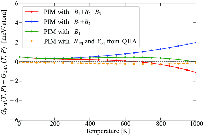
To evaluate the accuracy of PIM, we compared the Gibbs free energy obtained by Eqs. (14)(16) () and the one by QHA () as shown in Fig. 1. The red, blue, and green lines are the calculated with Eqs. (14)(16). Our method can calculate the Gibbs free energy within meV/atom of QHA up to 1000 K, even for fcc-Al, where the contribution of thermal expansion is large. The green line based on in Eq. (14) shows a good agreement with compared with the red and bule lines. This is thought to be due to the cancellation between and . As a supplement, we show the dashed yellow line where the PIM was performed using and obtained by QHA. There is an error originated from the second-order EOS, but this error can be ignored.
IV Summary
We have proposed an alternative approach to calculate the change in the Helmholtz free energy due to thermal expansion from phonon calculations and Grüneisen parameters. We have applied our method to fcc-Al with large thermal expansion and achieved an accuracy of a few meV/atom up to 1000 K. Because of the low cost of our method, we expect it to be very useful for high-throughput phase diagram calculations based on first-principles calculations in the future.
Acknowledgements.
This work was partly supported by JSPS-KAKENHI Grant No. 24K01144 and by MEXT-DXMag Grant No.JPMXP1122715503. The calculations were partly carried out by using supercomputers at ISSP, The University of Tokyo, and TSUBAME, Tokyo Institute of Technology.Appendix A FORCE CONSTAMTS AND GRÜNEISEN PARAMETER
If the atomic displacements are small compared with the interatomic distance, the potential energy where is the atomic position of the interacting atomic system can be expanded in a power series of the displacements as follows:
| (17) | ||||
| (18) |
where and is the displacement of atom in the th unit cell. In. Eq. (18) the linear term is omitted because atomic forces are zero in equilibrium positions. The coefficient defined as
| (19) |
are called the th order interatomic force constants in real-space representation. The phonon frequency can be obtained by diagonalizing dynamical matrix as
| (20) |
where is the polarization vector and is the atomic mass of atom and is the translational vector of the th unit cell. Grüneisen parameter in Eq. (10) is derived from the change in the dynamical matrix as
| (21) | ||||
| (22) | ||||
| (23) |
References
- Liu [2023] Z.-K. Liu, Calphad 82, 102580 (2023).
- Kikuchi [1951] R. Kikuchi, Physical Review 81, 988 (1951).
- Van Baal [1973] C. M. Van Baal, Physica 64, 571 (1973).
- Sanchez and de Fontaine [1978] J. M. Sanchez and D. de Fontaine, Physical Review B 17, 2926 (1978).
- Sanchez et al. [1984] J. M. Sanchez, F. Ducastelle, and D. Gratias, Physica A: Statistical Mechanics and its Applications 128, 334 (1984).
- Mohri et al. [1985] T. Mohri, J. M. Sanchez, and D. De Fontaine, Acta Metallurgica 33, 1463 (1985).
- Kikuchi [1994] R. Kikuchi, Progress of Theoretical Physics Supplement 115, 1 (1994).
- Dove [1993] M. T. Dove, Introduction to Lattice Dynamics (Cambridge University Press, 1993).
- Mauger et al. [2014] L. Mauger, M. S. Lucas, J. A. Muñoz, S. J. Tracy, M. Kresch, Y. Xiao, P. Chow, and B. Fultz, Physical Review B 90, 064303 (2014).
- Tanaka and Gohda [2020a] T. Tanaka and Y. Gohda, Journal of the Physical Society of Japan 89, 093705 (2020a).
- Tanaka and Gohda [2020b] T. Tanaka and Y. Gohda, npj Computational Materials 6, 1 (2020b).
- Pavone et al. [1993] P. Pavone, K. Karch, O. Schütt, D. Strauch, W. Windl, P. Giannozzi, and S. Baroni, Phys. Rev. B Condens. Matter 48, 3156 (1993).
- Karki et al. [2000] B. B. Karki, R. M. Wentzcovitch, S. de Gironcoli, and S. Baroni, Phys. Rev. B Condens. Matter 61, 8793 (2000).
- Mounet and Marzari [2005] N. Mounet and N. Marzari, Phys. Rev. B Condens. Matter 71, 205214 (2005).
- Ritz and Benedek [2018] E. T. Ritz and N. A. Benedek, Phys. Rev. Lett. 121, 255901 (2018).
- Togo et al. [2010] A. Togo, L. Chaput, I. Tanaka, and G. Hug, Phys. Rev. B Condens. Matter Mater. Phys. 81 (2010).
- Hellman et al. [2013] O. Hellman, P. Steneteg, I. A. Abrikosov, and S. I. Simak, Physical Review B 87, 104111 (2013).
- Hellman and Abrikosov [2013] O. Hellman and I. A. Abrikosov, Physical Review B 88, 144301 (2013).
- Romero et al. [2015] A. H. Romero, E. K. U. Gross, M. J. Verstraete, and O. Hellman, Physical Review B 91, 214310 (2015).
- Kadkhodaei et al. [2017] S. Kadkhodaei, Q.-J. Hong, and A. van de Walle, Physical Review B 95, 064101 (2017).
- Kadkhodaei and van de Walle [2020] S. Kadkhodaei and A. van de Walle, Computer Physics Communications 246, 106712 (2020).
- Souvatzis et al. [2008] P. Souvatzis, O. Eriksson, M. I. Katsnelson, and S. P. Rudin, Physical Review Letters 100, 095901 (2008).
- Tadano and Tsuneyuki [2015] T. Tadano and S. Tsuneyuki, Phys. Rev. B Condens. Matter 92, 054301 (2015).
- Tadano and Tsuneyuki [2018] T. Tadano and S. Tsuneyuki, J. Phys. Soc. Jpn. 87, 041015 (2018).
- Quong and Liu [1997] A. A. Quong and A. Y. Liu, Phys. Rev. B Condens. Matter 56, 7767 (1997).
- van de Walle and Ceder [2002] A. van de Walle and G. Ceder, Rev. Mod. Phys. 74, 11 (2002).
- Zhang et al. [2013] B. Zhang, X. Li, and D. Li, CALPHAD 43, 7 (2013).
- Wang et al. [2010] Y. Wang, J. J. Wang, H. Zhang, V. R. Manga, S. L. Shang, L.-Q. Chen, and Z.-K. Liu, J. Phys. Condens. Matter 22, 225404 (2010).
- Togo and Tanaka [2015] A. Togo and I. Tanaka, Scr. Mater. 108, 1 (2015).
- Ritz et al. [2019] E. T. Ritz, S. J. Li, and N. A. Benedek, J. Appl. Phys. 126, 171102 (2019).
- Masuki et al. [2022] R. Masuki, T. Nomoto, R. Arita, and T. Tadano, Phys. Rev. B Condens. Matter 105, 064112 (2022).
- Masuki et al. [2023] R. Masuki, T. Nomoto, R. Arita, and T. Tadano, Phys. Rev. B Condens. Matter 107, 134119 (2023).
- Grüneisen [1912] E. Grüneisen, Ann. Phys. 344, 257 (1912).
- Birch [1938] F. Birch, J. Appl. Phys. 9, 279 (1938).
- Birch [1947] F. Birch, Phys. Rev. 71, 809 (1947).
- Katsura and Tange [2019] T. Katsura and Y. Tange, Minerals 9, 745 (2019).
- Fletcher and Yahaya [1979] G. C. Fletcher and M. Yahaya, J. Phys. F: Met. Phys. 9, 1529 (1979).
- Kittel [2018] C. Kittel, Kittel’s Introduction to Solid State Physics, Global Edition, 8th Edition (Wiley, 2018).
- Mei et al. [2009] Z.-G. Mei, S. Shang, Y. Wang, and Z.-K. Liu, Phys. Rev. B Condens. Matter 79, 134102 (2009).
- Ashcroft and Mermin [2011] N. W. Ashcroft and N. D. Mermin, Solid State Physics (Cengage Learning, 2011).
- Blöchl [1994] P. E. Blöchl, Phys. Rev. B Condens. Matter 50, 17953 (1994).
- Kresse and Furthmüller [1996] G. Kresse and J. Furthmüller, Phys. Rev. B Condens. Matter 54, 11169 (1996).
- Kresse and Joubert [1999] G. Kresse and D. Joubert, Phys. Rev. B Condens. Matter 59, 1758 (1999).
- Perdew et al. [1996] J. P. Perdew, K. Burke, and M. Ernzerhof, Phys. Rev. Lett. 77, 3865 (1996).
- Tadano et al. [2014] T. Tadano, Y. Gohda, and S. Tsuneyuki, J. Phys. Condens. Matter 26, 225402 (2014).