Construction and sampling of alloy cluster expansions — A tutorial

Abstract

Crystalline alloys and related mixed systems make up a large family of materials with high tunability which have been proposed as the solution to a large number of energy related materials design problems. Due to the presence of chemical order and disorder in these systems, neither experimental efforts nor ab-initio computational methods alone are sufficient to span the inherently large configuration space. Therefore, fast and accurate models are necessary. To this end, cluster expansions have been widely and successfully used for the past decades. Cluster expansions are generalized Ising models designed to predict the energy of any atomic configuration of a system after training on a small subset of the available configurations. Constructing and sampling a cluster expansion consists of multiple steps that have to be performed with care. In this tutorial, we provide a comprehensive guide to this process, highlighting important considerations and potential pitfalls. The tutorial consists of three parts, starting with cluster expansion construction for a relatively simple system, continuing with strategies for more challenging systems such as surfaces and closing with examples of Monte Carlo sampling of cluster expansions to study order-disorder transitions and phase diagrams.

I Introduction

Materials engineering proposes a solution to many of the energy related problems our society is faced with. Tremendous research efforts are currently put towards optimizing green technologies such as solar cells, batteries, catalysts and fuel cells. The performance of these technologies is dictated by the properties of the materials involved, meaning that optimization is achieved by improving the materials design, which in turn requires tunability of the materials. A common strategy to expand the tunability is to consider multicomponent systems, since the larger chemical space enables tailoring via chemical composition and ordering. Recent examples can be found in the fields of photovoltaics [1, 2, 3, 4, 5], batteries [6, 7, 8], catalysis [9, 10, 11], fuel cells [12, 13], nanophotonics and nanoplasmonics [14, 15], construction and manufacturing [16, 17, 18, 19] as well as two-dimensional materials such as MXenes [20, 21, 22, 23].

The increased tunability comes at the cost of added complexity in the materials design process and computational methods are often needed to efficiently span the composition space. While computational efforts are ideally based on ab-initio methods such as density-functional theory (DFT) calculations, such methods are typically computationally too expensive for sampling the relevant composition space. To exemplify, a binary system consisting of $N$ atoms corresponds to approximately $2^{N}$ indistinguishable atomic configurations, meaning that already at system sizes of $100$ atoms one would need to examine roughly $10^{30}$ atomic configurations. For this reason, more effective models are necessary. For crystalline materials, cluster expansions (CEs) are ideal candidate models as indicated by the large number of successful applications including phase diagram prediction for metals [24, 25, 26, 27, 28] and semiconductors [29, 30, 31, 32, 33], ordering phenomena [34, 35, 36, 37, 38, 39, 40] as well as the properties of surfaces [41, 42, 43, 44, 45, 46, 47, 48, 49, 50, 51] and nanoparticles [52, 53, 54, 55, 56, 57, 58, 59].

Figure 1: Constructing and sampling a CE. An overview of the typical procedure of constructing and sampling a CE and a connection to the three main parts of this tutorial.

CEs are generalized Ising models that can in principle predict the energy (or any other function of the configuration) of any atomic configuration after training on only a small subset of the available atomic configurations (Fig. 1). They are typically sampled in Monte Carlo (MC) simulations to extract thermodynamic information about the system and study thermodynamic observables such as chemical ordering, free energy and heat capacity. CEs are not limited to energy prediction and have also been used to model, for example, activation barriers [60], vibrational properties [61, 62], chemical expansion [38] and transport properties [37, 63]. There are many software packages that implement the CE framework and thermodynamic sampling via MC sampling, including, e.g., atat [64], uncle [65], clease [66], casm [67], icet [68] and smol [69].

In this tutorial, we present an overview on practical aspects to consider when constructing and sampling CEs. It is accompanied by a set of jupyter notebooks available online (https://ce-tutorials.materialsmodeling.org [70, 71]) that use the icet package [68]. The tutorial is organized as follows. First, the CE formalism is briefly outlined in Sect. II. Second, we review the CE construction process for a relatively simple system (Mo_1-xV_xC_1 - y□_y) in Sect. III, with emphasis on training set generation and training procedure. Next, we discuss CE construction for a low symmetry system, namely a Au_xPd_1-x surface, in Sect. IV, which allows us to discuss the use of local symmetries, Bayesian priors and constraints for improving CE performance. Lastly, in Sect. V we introduce sampling of CEs via MC simulations to obtain various thermodynamic observables for Au_3Pd as well as the Ag_xPd_1-x alloy system.

II Cluster expansion formalism

The theory behind CEs has been discussed at length elsewhere [72, 30, 73, 74, 75, 76, 77]. In the present context, we present a short overview and focus on practical considerations.

A CE predicts the value of some observable $E$ as a function of the atomic configuration, represented by the occupation vector $\bm{\sigma}$, for a crystalline material, based on all involved atomic clusters $\bm{\alpha}$. A cluster is a set of $k$ atomic sites on the crystalline lattice where $k=0,1,2,\ldots$ is the order of the cluster. The observable can be expressed as

$$E(\bm{\sigma})=\sum_{\bm{\alpha}}J_{\bm{\alpha}}\Pi_{\bm{\alpha}}(\bm{\sigma}),$$ (1)

where $J_{\bm{\alpha}}$ is the contribution of cluster $\bm{\alpha}$, called the effective cluster interaction (ECI), and $\Pi_{\bm{\alpha}}$ are orthogonal basis functions spanning the space of atomic configurations [72, 76]. All symmetrically equivalent clusters have the same ECI and can be grouped into what we will refer to as an orbit (originating from group theory and used in [68]), which is also referred to as a representative cluster in the CE literature. Exploiting this fact simplifies Eq. (1) to

$$E(\bm{\sigma})=\sum_{\bm{\alpha}}m_{\bm{\alpha}}J_{\bm{\alpha}}\langle\Pi_{\bm{\alpha}^{\prime}}(\bm{\sigma})\rangle,$$ (2)

where $m_{\bm{\alpha}}$ is the multiplicity of orbit $\bm{\alpha}$ and the basis function $\Pi_{\bm{\alpha}}$ is averaged over all clusters in the orbit. The sum in Eq. (2) runs over all orbits up to some cutoff criterion, typically defined by a cutoff radius $r$ for each cluster order $k$.

Training a CE involves finding the optimal ECIs based on a set of atomic structures for which the value of the observable $E$ is known, called the training set. In most cases, $E$ is the energy obtained from DFT calculations. Equation (2) can be cast as a linear problem,

$$\bm{y}=\bm{X}\bm{w},$$ (3)

where $\bm{y}$ is a vector comprising the target values of the observable $E$ for the training set, $\bm{w}$ is an unknown vector containing the ECIs, and $\bm{X}$ is the so-called sensing matrix, where each row correspond to the values of the basis functions $\Pi_{\bm{\alpha}}$ for a structure in the training set. Note that in this form the multiplicities are absorbed into either $\bm{y}$ or $\bm{X}$.

The optimal ECIs $\bm{w}_{\text{opt}}$ can be found using linear regression techniques (see subsection III.1). Once the optimal ECIs are found, the CE can be used to predict $E$ for any atomic configuration representable by a supercell of any size and concentration.

The CE formalism applies to ideal lattices. In most cases, however, relaxed structures are more thermodynamically relevant than structures with atoms residing precisely on the lattice sites. CEs are therefore often used to model the energy of relaxed structures mapped to the closest corresponding occupation on the ideal lattice. This means that the ECIs effectively include variations in the interactions due to volume changes and atomic relaxations.

The validity of a CE employed over a concentration range has been debated in the literature [73, 78, 79]. In practice, for rare cases, it can become difficult to model the full concentration range with a single CE, especially if the system, for example, undergoes a sharp transition at some specific concentration. There are also cases were CEs may not be sufficient to capture all relevant interactions in the system, such as long-ranged strain interactions which requires extending the CE formalism to reciprocal space [80, 25, 81].

III Part 1: A first example

In the first part of this tutorial, we illustrate the construction of a CE using different regression techniques and approaches to structure selection. To this end, we consider a simple carbide Mo_1-xV_xC_1 - y□_y with two sublattices on a rocksalt lattice. On the metal sublattice we consider mixing between Mo and V, and on the carbon sublattice we consider C atoms and vacancies ($\square$), with a maximum of 30% carbon vacancies. We employ cutoffs of 9 and 5 for two and three-body clusters, respectively. This yields a total number of 52 ECIs, including two singlets, 25 pairs, 24 triplets as well as a constant, sometimes referred to as the zerolet.

The cutoffs for a CE need to be selected with some care, because using too short cutoffs can lead to underfitting while too long cutoffs can lead to overfitting. Here, we use a simple scan over a range of cutoffs and select optimal values based on the accuracy of the model (see details in the demonstration notebooks [70, 71]). In general one should study the property of interest (e.g., phase diagram, heat capacity etc.) for various cutoffs to make sure that convergence is achieved. It should, however, be noted that with proper regularization, the choice of cutoffs is less important, as will become apparent in subsection III.1.

The two main considerations when constructing a CE is (i) how to solve the linear problem in Eq. (3) and (ii) which atomic structures to include in training set. In the following, we discuss these two topics. To this end, we use reference data from DFT calculations available online [71]. The computational details concerning these calculations can be found in Appendix A.

III.1 Regression methods

There are many approaches to solving the linear regression problem in Eq. (3) [82, 83, 68, 84, 85]. Here we provide a short introduction to several common methods.

The solution of the linear problem, Eq. (3), with regularization can be written as

$$\bm{w}_{\text{opt}}=\underset{\bm{w}}{\text{argmin}}\left\{\|\bm{X}\bm{w}-\bm{y}\|^{2}_{2}+\bm{w}^{T}\bm{\Lambda}\bm{w}+\beta\|\bm{M}\bm{w}\|_{1}\right\},$$ (4)

where $\bm{w}_{\text{opt}}$ is the solution, $\bm{\Lambda}$ is the $\ell_{2}$ regularization matrix and $\bm{M}$ is the $\ell_{1}$ regularization matrix. Setting $\bm{\Lambda}=\bm{M}=\bm{0}$ yields the ordinary least squares (OLS) solution. OLS is, however, prone to overfitting, meaning that the model captures noise in the training data (resulting in a low training error) and therefore performs poorly on new unseen data (as indicated by a large validation error). For $\bm{M}=0$ and $\bm{\Lambda}=\alpha\bm{1}$, Eq. (4) reduces to ridge regression with regularization parameter $\alpha$, and with $\bm{\Lambda}=0$ and $\bm{M}=\alpha\bm{1}$ one obtains the expression used in least absolute shrinkage and selection operator (LASSO).

The regularized regression methods generally assume that the sensing matrix, $\bm{X}$, is standardized. Therefore, it is common practice to rescale the columns of $\bm{X}$ to have unit variance before solving the problem, and afterwards apply the inverse procedure to obtain the unscaled parameters. This rescaling needs to be taken into consideration if manually choosing values for the regularization matrices $\bm{\Lambda}$ and $\bm{M}$ (for instance for Bayesian CEs, see subsection IV.2). Additionally, one commonly trains CEs for the mixing (or formation) energy, rather than the total energy in order to avoid very large target values, $\bm{y}$.

Feature selection techniques can be used to reduce the number of nonzero ECIs in the solution vector. This can lead to more transferable models and faster predictions (e.g., in MC simulations). Recursive feature elimination (RFE) is an iterative algorithm where in each iteration, one solves the linear problem (typically with OLS) and the least important (smallest) ECIs are pruned (set to zero). This is iterated until a desired number of nonzero ECIs is reached. Automatic relevance detection regression (ARDR) is based on the Bayesian ridge regression technique where the regularization matrix is diagonal with elements $\Lambda_{ii}=\lambda_{i}$. The individual regularization strengths $\lambda_{i}$ for each parameter are updated throughout the optimization, and parameters are pruned (set to zero) if $\lambda_{i}$ increases above a threshold ($\lambda$-threshold) [86]. These linear regression methods can readily be employed for CEs using icet via scikit-learn [87] or even more directly via the trainstation interface to the former [84].

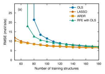
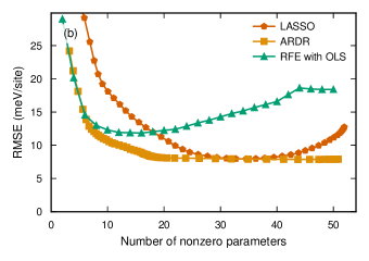
Figure 2: RMSE using different regression methods in the Mo_1-xV_xC_1 - y□_y system. (a) The validation RMSE based on the random training set using different regression methods as a function of the number of structures included in the training set. (b) The validation RMSE when using 80 training structures as a function of the number of nonzero parameters obtained after regression and feature selection. Here, the number of nonzero parameters obtained is controlled by varying the hyperparameter controlling the sparsity of the solution continuously. For ARDR this is the $\lambda$-threshold parameter, for LASSO it is $\alpha$ (see Eq. (4)) and for RFE it is the number of features.

Let us now explore some of the above mentioned regression methods for solving Eq. (3) in order to illuminate some of their differences. For the sake of simplicity we consider a set of 200 “random” training structures, where each structure has a randomized supercell size (up to maximum 50 atoms), random Mo/V and C/vacancy concentrations, and random occupation of the lattice. This set of structures will be referred to as the random set of structures from here on out. In order to evaluate the accuracy or performance of a model one typically uses cross-validation (CV) to obtain a validation (root mean square) error, as studying the training error is often a poor estimate of how the model will perform on unseen data points outside the training set. The resulting validation error as a function of number of training structures is shown in Fig. 2a). First, we note that all four regression methods yields similar validation errors when using a large training set. For OLS the validation error increases rapidly when decreasing the number of training structures, which is also to lesser extent the case for RFE, due to overfitting. Both ARDR and LASSO perform significantly better than OLS and RFE when using a small number of training structures.

ARDR, RFE, and LASSO all have one hyperparameter that controls the sparsity (number of nonzero parameters in the solution), which needs to be chosen. This is typically done by scanning over the hyperparameter value and selecting the value yielding the smallest validation error. Here, we use this procedure each time a model is trained. There are other metrics that can be used in place of the validation error, for example information criteria such as alkaline information criteria (AIC) and Bayesian information criterion (BIC) [88, 89, 90, 91].

Fig. 2b shows an example for the variation of the validation error with the resulting number of features during a hyper parameter scan. LASSO has a minimum at about 35 nonzero-parameters whereas ARDR achieves the same validation error with only 20 parameters. The tendency of LASSO to over-select is known [92] and we have observed this behavior previously for both CEs [68] and in other applications such as force constant expansions [84]. RFE has a minimum at about 15 nonzero-parameters but with slightly higher validation error compared to the other two regression methods.

The trends described above are rather general, and we have found in particular ARDR to be usually the most performant approach. Therefore, we recommend using ARDR as a starting point for CE construction. More advanced CE construction techniques are discussed in Sect. IV.

III.2 Training set generation methods

Let us now consider the choice of training structures. In subsection III.1 randomized structures were used. Structures generated in this fashion are often similar to each other, or, in mathematical terms, strongly correlated and do not span the cluster-vector space efficiently, i.e., there are only small variations in the sensing matrix columns. In a binary system, for example, we want to span the cluster-vector space between the two pure phases represented by $\bm{\Pi}=[1,1,1,\ldots]$ and $\bm{\Pi}=[-1,-1,-1,\ldots]$, but large randomized supercells predominantly have concentrations around 50% and $\bm{\Pi}\approx[0,0,0,\ldots]$.

Figure 3: Structure generation and selection schemes. The process of generating and selecting a set of structures for the training set can be designed in multiple ways. In this tutorial, we focus on the five approaches represented by the arrows in this schematic overview.

There are many methods for generating a set of training structures, each having their own pros and cons. Strictly speaking, one should discriminate between structure generation and selection:

In this tutorial, we consider four ways of generating structures; enumeration of all possible structures up to some maximum structure size, randomized structures (in terms of structure size, composition and/or configuration), MC sampling (seeSect. V) of existing CEs and selecting one (or a set of) target cluster vector(s) and finding the closest matching structure(s).

We also consider four ways of selecting structures. The most straightforward choice is to select all the generated structures, which leaves little control of the quality of the training set. More advanced selection methods can be applied with the aim of optimizing some aspect of the training set, such as minimizing the condition number of the sensing matrix, selecting structures with the largest uncertainty or trying to achieve a set of structures with orthogonal cluster vectors.

These generation and selection schemes can be combined and modified to create a sheer endless number of different training sets. Here, we consider five approaches which we refer to as uncertainty maximization, condition number minimization, structure orthogonalization, structure enumeration as well as the random set discussed in subsection III.1 (Fig. 3). In the following, we will present and discuss these approaches. Note that in practice, combining structures from these approaches might be a good idea, as well as including ground-state structures since these are often thermodynamically very relevant structures.

Uncertainty maximization is a form of active learning which is a common training set generation approach for model construction in general. Here, the model is iteratively trained and new structures are selected at each iteration based on the model uncertainty prediction for a pool of structures. The uncertainty of structures can be estimated from, for example, an ensemble of CEs from bootstrap sampling [68, 93]. This means that a collection of CEs trained in identical fashion but based on different training sets is generated. The different training sets are generated by resampling the original training set with replacement (meaning one structure can appear multiple times in a training set). Structures can, e.g., be generated using MC simulations in the canonical ensemble (see Sect. V) and the ones with the largest uncertainties are selected to be included in the training set. The benefit of this structure generation approach is that the training structures added during each iteration are structures for which the current ensemble of models predicts large uncertainty, and therefore will lead to large accuracy improvements in each iteration. Another benefit of this approach is that structures are generated from MC simulations with the desired conditions (concentrations, temperatures etc.) meaning the structures selected will be thermodynamically relevant ones. On the other hand, this also limits the pool of structures to select from in terms of how they span the cluster vector space. Furthermore, this approach requires a relatively large effort due to the iteration process and the fact that one needs to define a set of structures for which the uncertainty is predicted.

Condition number minimization refers to the process of selecting structures such that the condition number of the linear problem in Eq. (3) is minimized. The condition number $c$ is defined as [94]

$$c=\frac{\text{max}(\Gamma)}{\text{min}(\Gamma)},$$ (5)

where $\Gamma$ are the singular values of the sensing matrix. The condition number describes how well conditioned the linear problem is, with smaller values indicating better conditioning. It can be thought of as a measure of how sensitive the fitting result is with respect to changes or errors in the input data.

This approach starts by generating a large pool containing on the order of millions of randomly generated structures. An initial training set of $N$ structures is randomly drawn from the pool, where $N$ is on the order of hundreds. Next, a simulated annealing MC simulation (see Sect. V) is carried out where structures from the large random pool are randomly swapped in and out of the training set with probability $P=\mathrm{e}^{-\Delta c/\Theta}$ where $\Theta$ is an artificial temperature and $\Delta c$ is the change in condition number when swapping two structures. The resulting training set will be an approximate solution to the problem of selecting a subset of $N$ structures from the large pool with the lowest condition number.

Figure 4: Correlations between orbits. Correlations between (a) the singlets of the carbon (A) and metal (B) sublattices and (b) the metal singlet and nearest neighbor. The light grey area indicates the available space represented by all the structures from the large random pool used for condition number minimization. The orthogonal data set is shown in orange. The orthogonalization procedure is visualized by the initial (circle) and final (star) positions of three example structures.

Structure orthogonalization aims at providing a set of structures with cluster vectors orthogonal to each other [95, 82]. It is related to the condition number approach described above in the sense that both methods aim to span the cluster-vector space. The procedure starts from a structure with a random cluster vector. New structures are then added iteratively by finding a cluster vector that is orthogonal to the rest and identifying the closest matching structure.

A benefit with this approach is that, in principle, one can quickly produce a training set without the need for any iterative models (as in the uncertainty maximization) or large pool of structures (as in the condition number minimization). The latter depends, however, on the ability to find a matching structure for a target cluster vector without, e.g., a pool of structures. In icet, this is possible due to an implemented method based on simulated annealing.

There are, however, two major drawbacks to this approach. First, the entire cluster vector space is not available due to correlations between the cluster vector elements (Fig. 4). For instance, the number of possible A–B nearest neighbor pairs is limited by the value of the singlet. We show this in Fig. 4 for the entire available space (represented by the large random pool used for condition number minimization) and the data set produced using this approach. Clearly, both the fact that the concentration range for the carbon sublattice is restricted and that the singlet and pairs are correlated significantly limits the available space. The orthogonalization procedure will more often than not ask for a structure outside of this space and the resulting structure (with the closest matching cluster vector) will not be orthogonal to the other structures.

Second, the number of orthogonal cluster vectors is limited by the number of elements in the cluster vector (which in turn is determined by the cutoffs). This means that the training set size is limited by the cluster cutoffs when using this approach.

Structure enumeration is a method that generates all symmetrically inequivalent structures that are permissible given a certain lattice, under the constraint that the number of atoms in each structure must be smaller than some given number [96]. The benefit of structure enumeration is that it requires no other input than the maximum number of atoms in a supercell and will systematically generate high-symmetry and ground-state structures. One drawback is that the maximum number of atoms needs to be quite small (typically less than 15 atoms) in order for the number of structures to be computationally feasible, and this can lead to the training set not spanning long-ranged interactions. For our model system, Mo_1-xV_xC_1 - y□_y (with the chosen cutoffs), enumeration up to 12 atoms leads to about 650 structures, but produces an ill-conditioned sensing matrix and should thus not be used for training. For this reason, the enumerated training set is here only used for testing purposes. Additionally, for systems with larger and/or complex primitive cells, it may be unfeasible to use altogether as the number of enumerated structures grows exponentially with the size of the primitive cell.

Figure 5: Comparison of structure generation schemes for the Mo_1-xV_xC_1 - y□_y system. The RMSE over the different structure sets when training with the random training set, the uncertainty training set, the condition number training set and the orthogonal training set. Training is done with 110 structures using (a) OLS and (b) ARDR. The RMSEs are obtained by CV. The dashed line here indicates the average over the five structure sets.

Before we compare these approaches, let us note that the validation error is not a suitable measure to evaluate the quality of a training set generation scheme, because a procedure generating very similar (or identical) structures would lead to models with low validation errors but poor predictions on structures outside the training set. Therefore, we evaluate each CE on all the structures sets generated (Fig. 5).

In Fig. 5a the validation error is shown over all sets of structures for CEs trained with each training set using OLS. Here, we see that the random training set leads to larger errors across all structure sets, whereas training using the three other structure sets yields lower validation errors across the board. In Fig. 5b the same analysis is carried out for training with ARDR. Here, we see that the validation errors obtained with a random training set are on the same level as the other training sets, demonstrating the efficacy of ARDR even with a poor choice of training structures. We also note that training with the structure orthogonalization structures leads to a large error over the condition number structures, yet very small validation error, indicating poor transferability.

III.3 Conclusions

In the first part of this tutorial, we have demonstrated the CE construction process for a relatively simple system, focusing on linear regression and structure generation and selection. We have found that OLS with a training set consisting of randomized structures leads to large validation errors, and that this can be prevented by using better structure selection schemes as well as regularization and feature selection. We note that the material considered here presents a rather simple system with high symmetry and for more complex cases, optimizing the training set and regression method typically yields a larger benefit.

Based on these findings, we recommend generating structures via either uncertainty minimization (if it seems worthwhile to put in the effort) or condition number minimization (if you want to avoid an iterative process) in conjunction with ARDR when solving the linear problem Eq. (3).

IV Part 2: Low-symmetry systems

Figure 6: Merging of orbits. Side view of a 12-layer FCC-(111) surface slab. The numbers on the left row of atoms indicate the symmetrically inequivalent sites. Examples of orbits that can be merged if only site 1 is considered a surface site are marked with pink for pairs and green for triplets and different symbols for inequivalent orbits (note the difference in length between sets of pairs).

In the second part of this tutorial, we consider CE construction for a low-symmetry system, specifically a surface, which comes with new challenges. The number of orbits for a given set of cutoffs grows with the number of symmetrically inequivalent sites that make up the material. For simple bulk systems, such as the one in Sect. III, the unit cell typically comprises one or a few atoms which constitute the maximum number of inequivalent sites. For low-symmetry systems such as surfaces and nanoparticles, on the other hand, the unit cell is generally larger. For instance, the number of inequivalent sites for a surface slab is at least the number of layers divided by two (Fig. 6). Consequentially, the number of orbits increases rapidly with the number of layers and the CE construction procedure outlined in Sect. III can be insufficient.

In the following, we discuss three approaches to improve CE construction for low-symmetry systems. The first two approaches are based on grouping similar orbits and either explicitly merging them or coupling them in a Bayesian framework. The third approach consists of adding weighted constraints to ensure that specific properties are more accurately predicted. These approaches can be combined and are not restricted to low-symmetry systems.

To showcase these approaches we will construct CEs for a 12-layer Au_xPd_1-x FCC-(111) surface slab. The cutoffs used for CE construction are 6 and 3 for two and three-body clusters, respectively, resulting in 76 orbits. The training set consists of the pure Au and Pd slabs and 201 structures generated using the orthogonal cluster space approach described in subsection III.2 (using slightly larger cutoffs to avoid underdetermined systems during training). Details on the DFT calculations can be found in Ref. 50.

We begin by training CEs as in Sect. III, using plain OLS and ARDR to fit the ECIs. As expected, ARDR outperforms OLS in terms of the validation error as well as with respect to the number of structures necessary to reach convergence (Fig. 7).

Figure 7: Learning curves for a surface CE. The validation error as a function of the training set size for different linear regression methods, with and without merging of orbits.

The number of structures needed to reach convergence is, however, relatively large for both fitting methods.

The validation error is not always a sufficient measure for CE accuracy. In the present example of a surface, we find that although the validation energy has converged, the segregation energy prediction is associated with large errors, which will ultimately result in an erroneous predictions of the surface segregation. The segregation energy is the energy difference caused by moving, e.g., a single Pd atom in an otherwise pure Au slab from the middle of the slab (i.e., the bulk) to a site in the surface region. (Here, we construct 2x2x12 slabs for this purpose.) This calculation requires the prediction of two configurations which mean it is the relative error between these to configuration that matters. In Fig. 8a and d, we find that the segregation energies predicted by the plain OLS and ARDR CEs have large errors and systematically overestimate the energy gain of moving Pd (in Au) to the surface and the energy cost of moving Au (in Pd) to the surface. There are also unphysical oscillations of the segregation energy in the inner layers whereas the DFT results indicate that the segregation energy only varies in the outer 2 to 3 layers. This suggest that the models predict too large differences between the atoms in the inner layers, as discussed further in the following section.

Figure 8: Segregation energy predictions for surface CEs. Segregation energies for a single Pd atom in Au (upper panel) and a single Au atom in Pd (lower panel) positioned in each atomic layer calculated using DFT and predicted by different CEs. The layer index is counting from the surface, as in Fig. 6. (a, d) CEs trained using OLS and ARDR with and without merging of orbits. (b, e) CEs trained using Bayesian coupling of similar orbits. The CE with the optimal coupling parameter $\sigma_{\alpha\beta}$ from Fig. 9 is highlighted with triangles. (c, f) CEs trained with (unmerged) ARDR and an added constraint enforcing correct segregation energy prediction with increasing weight $\gamma$.

IV.1 Merging of orbits

At a sufficient distance from the surface, the atomic interactions should reach the bulk limit. For example, the energetic contribution from a nearest neighbour pair in layer 5 should be very similar to the one in layer 6. We can use this idea to introduce local symmetries. Orbits that belong to the same local symmetry should have the same ECI, which means that they can be merged into a single orbit. This process is analogous to when the individual clusters are grouped into orbits in Eq. (2). Note that it is important to be aware of the treatment of multiplicities when merging orbits to make sure that the merging is done correctly. There are multiple ways to define these local symmetries. In the following, we consider only the outermost layer as surface and treat the remaining layers as bulk. We then merge all orbits with the same order and radius that consist exclusively of bulk sites (Fig. 6), reducing the number of orbits from 76 to 20.

In Fig. 7 we see that this aggressive merging strategy leads to a significant reduction of the number of training structures necessary to reach a certain accuracy while actually improving the final validation error. Except for the smallest training set considered, there is almost no difference between OLS and ARDR. This is because the lack of regularization in OLS often leads to overfitting, which is avoided here due to the small number of features. We also find that the segregation energy predictions are significantly better for the merged CEs (Fig. 8a and d). This is a result of restricting the differences between the ECIs in the inner layers.

IV.2 Bayesian coupling of orbits

Figure 9: Performance of Bayesian surface CEs with varying coupling strength. Validation and training error with varying coupling parameter $\sigma_{\alpha\beta}$ for similar orbits. The validation error is shown for two different training set sizes (50 and 90%), and the training error is obtained using the full training set (100%). The optimal coupling parameter, $\sigma_{\alpha\beta}=0.2$, is highlighted with triangles.

The assumption that similar orbits should have similar energetic contribution to the total energy is an example of a physical insight about the system. If such insights can be formulated in the form of Bayesian priors, they can be used to construct improved CEs within a Bayesian framework [97, 98, 82]. Here, we follow the approach first presented by Mueller and Ceder in Ref. 97.

We assume Gaussian priors for the ECIs such that

$$P(\bm{w}|\bm{X})\propto\prod_{\alpha}e^{-w_{\alpha}^{2}/2\sigma_{\alpha}^{2}}\prod_{\alpha,\beta\neq\alpha}e^{-(w_{\alpha}-w_{\beta})^{2}/2\sigma_{\alpha\beta}^{2}},$$ (6)

where $P(\bm{w}|\bm{X})$ is the posterior. Here, the first product controls the magnitude of the ECIs via $\sigma_{\alpha}$ which is the standard deviation of the prior and should be chosen to roughly correspond to the expected value of the respective ECI. If one, for instance, wanted to achieve smaller ECIs for large clusters, one could define $\sigma_{\alpha}$ such that it decreases with orbit size. The second product controls the coupling between orbits via $\sigma_{\alpha\beta}$ which is the inverse coupling strength between orbits $\alpha$ and $\beta$.

Going back to the linear problem formulated in Eq. (4), the Bayesian priors are introduced via the $\ell_{2}$ regularization matrix $\Lambda$ which has diagonal elements $\Lambda_{\alpha\alpha}=\frac{\sigma^{2}}{\sigma_{\alpha}^{2}}+\sum_{\beta\neq\alpha}\frac{\sigma^{2}}{\sigma_{\alpha\beta}^{2}}$ and off-diagonal elements $\Lambda_{\alpha\beta}=\Lambda_{\beta\alpha}=-\frac{\sigma^{2}}{\sigma_{\alpha\beta}^{2}}$, where $\sigma$ reflects the typical error of the model. Then, the maximum posterior estimate for the ECIs is given by

$$\bm{w}_{\text{opt}}=(\bm{X}^{T}\bm{X}+\bm{\Lambda})^{-1}\bm{X}^{T}\bm{y}.$$ (7)

Similar to the merging approach, one has to be careful with the treatment of multiplicities when using Bayesian coupling of similar orbits. Coupling orbits means that we expect the values of their ECI to be similar. It is therefore crucial that the multiplicities are included in the sensing matrix and not the ECI vector when applying this approach. In addition, in linear regression one typically employs standardization, i.e., rescaling of the sensing matrix to improve the linear regression. If this is the case, one has to employ the same scaling of the Bayesian regularization matrix.

In this tutorial, we apply a rather simple Bayesian approach using the same definition of local symmetries as in Sect. IV and couple the orbits belonging to the same local symmetry using a single coupling parameter $\sigma_{\alpha\beta}$ for all coupled orbits. The ECI magnitude is controlled by a single value of $\sigma_{\alpha}$ for all orbits as well. We emphasize that the Bayesian priors can have a much more intricate design than this to allow for greater tunability [97]. For example, one can take into account the order and size of orbits and define complex criteria for the similarity of orbits.

In Fig. 9 we show how the validation and training error varies with the coupling parameter $\sigma_{\alpha\beta}$ while keeping $\sigma_{\alpha}=10$. For large $\sigma_{\alpha\beta}$, the unmerged CE is obtained with a high validation error but low training error (indicating overfitting). For small $\sigma_{\alpha\beta}$, the merged CE is recovered and the training and validation errors approach each other with a significant reduction of the validation compared to the large $\sigma_{\alpha\beta}$ limit. The latter is particularly prominent for smaller training sets. In between these to extremes, at about $\sigma_{\alpha\beta}=0.2$, the validation error has a minimum. This indicates that the optimal compromise between the freedom of unmerged orbits and reduced feature space of merged orbits is found. Fig. 8b and e show the segregation energy prediction for various values of $\sigma_{\alpha\beta}$.

The identified optimal $\sigma_{\alpha\beta}=0.2$ does provide some improvement in segregation energy prediction compared to the unmerged CEs, but decreasing $\sigma_{\alpha\beta}$ further towards the merged limit results in significantly better segregation energy prediction, in particular for the case of Pd in Au. This again shows that the validation RMSE is not always sufficient to find the most physically sound CE.

IV.3 Adding constraints and weights

A CE can also be manipulated by introducing constraints and/or weights to ensure that certain properties are reproduced more accurately. The property of interest depends on the purpose of the model. If, for example, the model is going to be used to study surface segregation phenomena, a natural choice is the segregation energy. Calculating the segregation energy requires DFT calculations of surface slabs with a single Pd atom in a Au slab, respectively positioned in each atomic layer, and vice versa resulting in a total of 12 structures. A straightforward approach to improve the segregation energy prediction is to include these structures in the training set. Additionally, one could give these structures a higher weight by simply multiplying the corresponding rows of the sensing matrix $\bm{X}$ and elements in the solution vector $\bm{y}$ with a suitably chosen factor. By doing so, the prediction error will shrink for these specific structures, effectively reducing the segregation energy error.

Another option, which we demonstrate in this tutorial, is to explicitly enforce better predictions of the segregation energy as a constraint. This entails reformulating the linear problem as

$$\begin{split}\bm{w}_{\text{opt}}=\underset{\bm{w}}{\text{argmin}}\big{\{}&\|\bm{X}\bm{w}-\bm{y}\|^{2}_{2}\\ &+\gamma\|(\bm{X}_{\text{S}}-\bm{X}_{\text{B}})\bm{w}-\bm{E}_{\text{seg}}\|^{2}_{2}\big{\}},\end{split}$$ (8)

excluding any regularization terms (see Eq. (4)). Here, $\bm{X_{\text{S}}}$ contains the cluster vectors of the structures with a single atom positioned in different atomic layers. Similarly, $\bm{X_{\text{B}}}$ contains the cluster vectors of the corresponding structures with a single atom in the bulk position (i.e., the innermost atomic layer). $\bm{E_{\text{seg}}}$ is the corresponding segregation energies and $\gamma$ is a weight factor that dictates how strongly the constraint is enforced.

In Fig. 8c and f, we show the segregation energy predictions for different weight factors $\gamma$. As expected, the segregation energy predictions move closer to the DFT line with increasing weight. The improvement in segregation energy prediction comes at the cost of a slightly increased validation error, from 2.8 for $\gamma=0$ to 3.4 for $\gamma=5$.

The strategy of introducing constraints and/or weights is not restricted to low symmetry systems and can be applied to any property that can be expressed as a function of the cluster vector. For example, one could constrain the mixing energy of the pure Au and Pd structures to be 0, give higher weight to structures close to some specific composition or use weights to compensate for an uneven sampling of the configuration space.

IV.4 Conclusions

In this section, we have presented three ways to adapt the CE construction process in order to achieve accurate models for complex systems, such as surfaces. These approaches should be seen as tools that can be used on their own (as shown here) or in conjunction and can be modified to provide a tailored solution for the problem at hand.

V Part 3: Monte Carlo sampling

In the third and last part of this tutorial, we show how the configuration space described by a CE can be sampled via MC simulations. This allows for calculation of thermodynamic observables such as free energies, order parameters and heat capacities. We will begin this section with a short introduction to MC simulations and the most common thermodynamic ensembles, and then illustrate these concepts using two examples.

V.1 Monte Carlo simulations

Thermodynamic sampling is usually carried out via Metropolis MC simulations [99] which are generally executed as follows. Starting from some arbitrary initial state, a so-called trial step is suggested, which consists of a change in the atomic configuration. This step is either accepted (i.e., implemented) or rejected according to the Metropolis criterion with a probability given by

$$\mathcal{P}=\min{\left\{1,\mathrm{exp}\left(-\Delta\psi/k_{B}T\right)\right\}},$$

where $\Delta\psi$ is the change in the relevant thermodynamic potential (which will be introduced further in subsection V.2). If the trial step is rejected, the system remains in its current state. The procedure is repeated until convergence is achieved.

V.2 Thermodynamic ensembles

MC simulations can be executed in different thermodynamic ensembles. The choice of which depends on the goal of the simulation and the properties to be extracted.

The canonical ensemble models a situation where the total number of particles ($N$) as well as their concentrations ($c_{i}$) are kept constant along with the temperature ($T)$. It thus represents a system free to exchange heat with a reservoir at temperature $T$.

Strictly speaking, in the canonical ensemble (and similarly in the semi-grand canonical (SGC) and variance-constrained semi-grand canonical (VCSGC) ensembles, see below) the volume ($V$) is constant. When constructing a CE one, however, commonly trains against configurations that have been relaxed with respect to both atomic positions and volume/cell shape. CE models trained in this fashion therefore incorporate the strain energy term that separates the canonical ($Nc_{i}VT$) from the isobaric-isothermal ensemble ($Nc_{i}Tp$). It is therefore more sensible to interpret the results of such CE-MC simulations in terms of the latter ensemble. In keeping with the literature, we will, however, use the terms for the constant-volume ensembles in the following.

The trial steps used to sample the canonical ensemble need to preserve the conserved quantities, specifically the concentrations of the different species ($c_{i}$). This can be accomplished by (simultaneously) swapping the occupancy of two sites. The change of the thermodynamic potential, $\psi$, is then given by the energy difference between the two states, i.e., $\Delta\psi=E_{\text{new}}-E_{\text{old}}=\Delta E$. In the context of this tutorial, $E$ refers to the energy predicted by the CE.

It is also possible to gradually reduce the temperature in an MC simulation in the canonical ensemble, an approach that is referred to as simulated annealing. This procedure be used as a general optimization algorithm, for example to find the lowest energy (ground-state) structures or in structure selection as implemented in subsection III.2.

The SGC ensemble refers to a case where the total number of particles ($N$) is fixed while the concentration of the different species is controlled via the relative chemical potentials ($\Delta\mu_{i}$), again at constant temperature ($T$). The SGC ensemble thus represents a system in connection with both a heat reservoir ($T$) and one or several particle reservoirs ($\Delta\mu_{i}$) under the constraint of a constant number of particles ($N$).

In the CE literature it is not uncommon for the SGC ensemble to be referred to as the grand canonical ensemble, which is, however, a misnomer. The actual grand canonical ensemble represents an open system that has no constraint on the total number of particles with the absolute chemical potentials ($\mu_{i}$) as variables [100]. By contrast, the semi-grand canonical ensemble represents a semi-open system, where the relative proportion of particles of different species but not their total number may change. In cases involving at least one sublattice with vacancies (such as the example discussed in Sect. III), one can interpret CE-based MC simulations in the SGC or VCSGC ensembles in terms of the grand canonical ensemble by imposing suitable thermodynamic boundary conditions. This approach is described and demonstrated in, e.g., Ref. 27, which also discusses para and full equilibria in this context.

As before, in the case of the canonical ensemble, trial moves used for sampling the SGC ensemble need to respect the respective constraints. A suitable trial move is therefore to change the occupation of a single site. The change in the thermodynamic potential is given by $\Delta\psi=\Delta E-N\sum_{i>1}\Delta c_{i}\Delta\mu_{i}$, where $N$ is the total number of sites, $c_{i}$ is the concentration of species $i$ and $\Delta\mu_{i}=\mu_{i}-\mu_{1}$ is the chemical potential difference of species $i$ relative to the first species.

A big advantage of the SGC ensemble compared to the canonical ensemble is that it directly connects to the derivative of the free energy per atom with respect to the concentration(s)

$$\frac{1}{N}\frac{\partial F}{\partial c_{i}}=-\Delta\mu_{i},$$

which can be integrated along the concentration axis (or axes) to yield the free energy. Inside multi-phase regions, the same chemical potentials map, however, to multiple different concentrations, which renders it impossible to integrate over (and in fact sample inside) miscibility gaps.

The VCSGC ensemble can, in contrast to the SGC ensemble, be used for sampling inside and across miscibility gaps [101]. Similar to the SGC ensemble it imposes a flexible constraint on the mean concentration(s) but unlike the SGC ensemble it also constrains their fluctuation(s). This is achieved via two variables, $\bar{\phi}$ and $\bar{\kappa}$, which control the mean and the variance of the concentration(s), respectively. The corresponding thermodynamic potential is given by $\Delta\psi=\Delta E+Nk_{B}T\bar{\kappa}(\Delta c+\bar{\phi}/2)^{2}$, and the ensemble can be sampled using the same kind of moves as those used for the SGC ensemble.

The free energy derivative per atom with respect to the concentration is given by

$$\frac{1}{N}\frac{\partial F}{\partial c}=-2k_{B}T\bar{\kappa}\left(\left<c\right>+\bar{\phi}/2\right)$$ (9)

As a result of the constraint on the variance of the concentration, one can also stabilize concentrations inside of miscibility gaps. This allows one to obtain the free energy as a continuous function of concentration, and thus enables free energy integration.

The choice of $\bar{\kappa}$ affects the strength of the variance constraint, corresponding to the inverse variance of the expected concentration. Larger values enforce smaller fluctuations, which reduces the acceptance ratios, requiring more sampling. Smaller values on the other hand, can cause the fluctuations to become too large to allow sampling two-phase regions as the VCSGC ensemble then approaches the SGC ensemble [101]. Empirically, we have found that $\bar{\kappa}=200$ strikes a good balance between sampling efficiency and quality for most systems.

We can get an idea for how to select suitable values for the parameter $\bar{\phi}$ by considering Eq. (9). For typical temperatures and values of $\bar{\kappa}$ the terms in front of the bracket on the right-hand side of Eq. (9) are much larger than the variation of the free energy on the left-hand side. As a result, we can assume that $2\left<c\right>+\bar{\phi}\approx 0$. It then follows that the concentration limits $\left<c\right>\rightarrow 0$ and $\left<c\right>\rightarrow 1$ are reached by setting $\bar{\phi}\approx-2-\delta$ and $\bar{\phi}\approx\delta$, respectively. Here, $\delta$ indicates that one needs to sample somewhat beyond those limits in order to cover the full composition range. In practice, a value of $\delta$ of about 0.3 is sufficient in most cases.

V.3 Ordering in Au3Pd using the canonical ensemble

As the first illustration we consider the order-disorder transition in AuPd3, which can be conveniently accessed via simulations in the canonical ensemble. Here, we use a CE developed in Ref. 27 for Au_1-xPd_x on the FCC lattice. In Fig. 10 we show the resulting long-range order parameter and heat capacity as a function of temperature. The long-range order is here represented by the partial static structure factor calculated between Pd atoms at $\mathbf{q}=\frac{2\pi}{a_{0}}[1,0,0]$ (see Eq. (11)), while the heat capacity is calculated via Eq. (10).

Figure 10: Order-disorder transition in AuPd3 from MC simulations. (a) Long-range order parameter and (b) heat capacity as a function of temperature and system size, where the solid lines are guides for the eye. The system size is given in multiples of the primitive (4-atom) unit cell. The long-range order is represented by the partial static structure factor between Pd-atoms. The inset shows the ordered low temperature phase.

The sharp peak in the heat capacity at approximately 175 indicates that the material undergoes a continuous phase transition from a disordered to an ordered phase (see inset in Fig. 10b) with decreasing temperature. The phase transition can also be seen in the long-range order parameter, as this is increasing sharply at the phase transition.

All simulations indicate a phase transition around 175, but there the sharpness of the transition is sensitive to supercell size, with larger systems yielding sharper transitions. This behavior is typical for continuous phase transitions, as the correlation length of the fluctuations in the systems diverges at the critical temperature [102]. In order to achieve convergence one therefore needs to consider a range of system sizes, and extrapolate to the infinite size limit if possible.

V.4 Phase diagram of Ag_xPd_1-x via the SGC and VCSGC ensembles

Next, we illustrate the construction of a phase diagram for a system with a miscibility gap, namely FCC Ag_xPd_1-x, using a CE from Ref. 68, a 10x10x10 supercell and MC simulations in both the SGC and VCSGC ensembles.

In the case of the SGC-MC simulations, the chemical potential was sampled using $105$ evenly spaced points between $-1.04$ and 1.04. For the VCSGC-MC simulations the variance constraint parameter $\bar{\kappa}$ was set to $200$, while the average constraint parameter $\bar{\phi}$ was varied between $-2.3$ and $0.3$ with $105$ evenly spaced points.

Figure 11: MC sampling of the Ag_xPd_1-x system. (a) Derivative of the free energy of mixing with respect to composition (i.e., the chemical potential), (b) free energy of mixing and (c) phase diagram. The inset in (b) shows the zoomed-in and tilted free energy of mixing in the vicinity of the miscibility gap (indicated by the blue diamonds). Due to the concave free energy at 400, the SGC-MC ensemble cannot form a stable solution. The miscibility gap is extracted from the free energy landscape of the VCSGC ensemble.

Miscibility gap. Figure 11a shows the free energy derivative obtained from sampling in both ensembles at a temperature below (400) and above (800) the miscibility gap. Here, the miscibility gap separates a Pd-rich phase containing almost no Ag, from a mixed phase with up to approximately 60% to 70% Pd.

Outside the miscibility gap, simulations in the SGC and VCSGC ensembles yields numerically identical results. In the SGC-MC simulations at 400 it is, however, apparent that the miscibility gap, i.e., the two-phase region between approximately 60% and 99%, is not accessible as the mapping between $\partial F/\partial c$ and the concentration $c$ is one-to-many (i.e., non injective), and the variance of the concentration diverges. In fact, here the identification of the free energy derivative with the relative chemical potential breaks down, as the latter is only meaningfully defined in single-phase regions.

When using SGC-MC simulations the free energy in the single-phase regions can still be obtained through thermodynamic integration starting from known limits such as in the low or high-temperature expansions [103]. Furthermore it is possible to obtain the phase diagram by tracing the phase boundaries [103]. To mitigate hysteresis effects, this requires iteratively sampling across two-phase regions as well as careful consideration of the convergence with respect to the numerical resolution of the chemical potential.

To counteract the divergence of the concentration in miscibility gaps, in the VCSGC ensemble one includes a term representing a constraint on the variance in the thermodynamic potential. This allows one to access also compositions inside the miscibility gap and sample the free energy derivative as a continuous function of composition (Fig. 11a). This in turn enables integrating the free energy over the entire concentration range (Fig. 11b). Finally, via the convex hull construction (inset in Fig. 11b) one can then readily extract the phase boundaries (Fig. 11c).

Thanks to the possibility to compute the free energy across two-phase regions one can furthermore extract excess free energies. Thereby, it is possible to compute, e.g., interface free energies as a function of interface orientation. The interested reader can find more information on this topic in, e.g., Refs. 101 and 81.

Finally, the VCSGC ensemble naturally enables an even sampling of the concentration axis as equidistant values of $\bar{\phi}$ leads to an approximately equidistant concentrations. This avoids adaptive sampling in the vicinity of phase transitions that are necessary when using the SGC ensemble.

Figure 12: Order-disorder transitions in Ag_xPd_1-x from VCSGC-MC simulations. (a) The heat capacity map reveals a continuous phase transition between a disordered and an ordered phase around 25% Pd. (b) The short-range order parameter [Eq. (12)] indicates the existence of a miscibility gap, however, it is hard to identify the exact boundaries. It also shows a sharp change at the order-disorder phase transition.

Secondary phase transitions. By mapping out the free energy, we were able to locate the miscibility gap in the Ag–Pd system. This phase boundary corresponds to a first-order phase transition as evident from the sudden (and discontinuous) transition in the derivative of the free energy with respect to composition. It is, however, very difficult (if not practically impossible for numerical reasons) to obtain information about continuous phase transitions. To this end, as we already saw above (subsection V.3) the heat capacity and order parameters are better suited.

Analysis of the heat capacity as a function of temperature and composition does indeed reveal a transition around 25% Pd and 200 (Fig. 12a). This transition closely resembles the one in Au3Pd that we analyzed before but here we also obtain the composition dependence of the transition. At 25% Pd the transition is very sharp, while both the heat capacity and the transition temperature drop with either decreasing or increasing composition. Note that the heat capacity shows no discernible features around the miscibility gap.

The order-disorder transition at around 25% Pd is also apparent from the short-range order parameter computed according to Eq. (12) (Fig. 12b). The short-range order map (unlike the heat capacity), however, also exhibits structure across the miscibility gap, which is the result of the variation in the proportions of the two different phases (Pd-rich and mixed). It is, however, clearly apparent that the short-range order is not suited for identifying the actual phase boundaries as the map is smooth and distinct features only emerge well inside the miscibility gap.

V.5 Conclusions

In the final part of this tutorial, we demonstrated the utility of MC simulations in different thermodynamic ensembles for extracting thermodynamic observables and identifying phase boundaries. Which ensemble is best suited depends on the task at hand. Generally speaking the canonical ensemble is simple to use (and understand) but limited in so far as it does not directly enable one to observe a first derivative of the free energy. It can still be used for thermodynamic integration (which was not covered here). The SGC and VCSGC ensembles both provide access to the first derivative of the free energy with respect to concentration and thereby can be used more readily for obtaining phase diagrams. The VCSGC ensemble additionally allows one to handily extract excess free energies. Here, we did not discuss acceptance ratios but in closing point out that while the canonical ensemble tends to yield higher acceptance ratios for small concentrations, the other two ensembles achieve higher ratios at higher concentrations [104].

VI Outlook

In this tutorial we have provided a short practical introduction into the topic of constructing and sampling CEs for the study of many-component systems. There are various more advanced topics that are beyond the scope of this tutorial that we invite so-inclined readers to pursue, including, e.g., handling sublattices [27], strain [80, 25, 81], ground state finding [105], materials under pressure [106], precipitate formation [107] or the description of migration barriers [60].

Appendix A Computational details

The DFT calculations for the simple carbide system, Mo_1-xV_xC_1 - y□_y, were carried out using the projector augmented method [108, 109] as implemented in vasp [110, 111, 112]. We used the van-der-Waals density functional method with consistent exchange [113, 114] for the exchange-correlation potential. The Brillouin zone was sampled with a $\Gamma$ centered $\mathbf{k}$-point grid, with the smallest allowed spacing between two k-grid points being $0.25\text{\,}\mathrm{\text{Å}}^{-1}$ and the plane wave cutoff energy $520\text{\,}\mathrm{e}\mathrm{V}$. Both the positions and cell were allowed to relax, the largest allowed residual forces were set to $0.02\text{\,}\mathrm{e}\mathrm{V}\mathrm{\text{Å}}^{-1}$.

Appendix B Thermodynamic properties

In addition to the properties mentioned above, one can obtain several other thermodynamic properties of interest from MC simulations.

The heat capacity is readily obtained via

$$C_{V}(T)=\frac{\mathrm{Var}[E(T)]}{k_{B}T^{2}},$$ (10)

where $\mathrm{Var}[E(T)]$ is the variance of the energy.

Long-range order can be assessed from the partial static structure factors, which are defined for atom types A and B as

$$S_{AB}(\bm{q})\propto\sum_{j}^{N_{A}}\sum_{k}^{N_{B}}\mathrm{exp}\left[-\mathrm{i}\bm{q}\cdot(\bm{R}_{j}-\bm{R}_{k})\right],$$ (11)

where $\bm{q}$ is a reciprocal lattice point and $\bm{R}_{k}$ the position of atom $k$.

Short-range order is often measured in terms of the Warren-Cowley short-range order parameter, which determines to which degree a binary (A-B) system mixes or segregates [115]. For an atom $i$ of type A it is defined as

$$\alpha_{i}=1-\frac{Z_{\text{B}}}{Z_{\text{tot}}c_{\text{B}}},$$ (12)

where $Z_{\text{B}}$ is the number of B neighbors in the first neighbor shell, $Z_{\text{tot}}$ is the total number of neighbors in the first shell and $c_{\text{B}}$ is the concentration of B atoms. For a random mixture we obtain $\alpha=0$, for a phase separated system we get $\alpha>0$, while $\alpha<0$ indicates ordering.

References

- Ma et al. [2009] W. Ma, J. M. Luther, H. Zheng, Y. Wu, and A. P. Alivisatos, Photovoltaic devices employing ternary \cePbS_xSe_1-x nanocrystals, Nano Letters 9, 1699–1703 (2009).
- Xiao et al. [2013] Z.-Y. Xiao, Y.-F. Li, B. Yao, R. Deng, Z.-H. Ding, T. Wu, G. Yang, C.-R. Li, Z.-Y. Dong, L. Liu, L.-G. Zhang, and H.-F. Zhao, Bandgap engineering , Journal of Applied Physics 114, 183506 (2013).
- Lu and Ferguson [2013] N. Lu and I. Ferguson, III-nitrides for energy production: photovoltaic and thermoelectric applications, Semiconductor Science and Technology 28, 074023 (2013).
- Feurer et al. [2016] T. Feurer, P. Reinhard, E. Avancini, B. Bissig, J. Löckinger, P. Fuchs, R. Carron, T. P. Weiss, J. Perrenoud, S. Stutterheim, S. Buecheler, and A. N. Tiwari, Progress in thin film CIGS photovoltaics – Research and development, manufacturing, and applications, Progress in Photovoltaics: Research and Applications 25, 645–667 (2016).
- Li et al. [2022] W. Li, X.-F. Cai, N. Valdes, T. Wang, W. Shafarman, S.-H. Wei, and A. Janotti, \ceIn2Se3, \ceIn2Te3, and \ceIn2(Se, Te)3 alloys as photovoltaic materials, The Journal of Physical Chemistry Letters 13, 12026–12031 (2022).
- Balogun et al. [2016] M.-S. Balogun, Y. Luo, W. Qiu, P. Liu, and Y. Tong, A review of carbon materials and their composites with alloy metals for sodium ion battery anodes, Carbon 98, 162–178 (2016).
- Lao et al. [2017] M. Lao, Y. Zhang, W. Luo, Q. Yan, W. Sun, and S. X. Dou, Alloy‐based anode materials toward advanced sodium‐ion batteries, Advanced Materials 29, 1700622 (2017).
- Song et al. [2019] K. Song, C. Liu, L. Mi, S. Chou, W. Chen, and C. Shen, Recent progress on the alloy‐based anode for sodium‐ion batteries and potassium‐ion batteries, Small 17, 1903194 (2019).
- Singh and Xu [2013] A. K. Singh and Q. Xu, Synergistic catalysis over bimetallic alloy nanoparticles, ChemCatChem 5, 652–676 (2013).
- Hannagan et al. [2020] R. T. Hannagan, G. Giannakakis, M. Flytzani-Stephanopoulos, and E. C. H. Sykes, Single-atom alloy catalysis, Chemical Reviews 120, 12044–12088 (2020).
- Nakaya and Furukawa [2022] Y. Nakaya and S. Furukawa, Catalysis of alloys: Classification, principles, and design for a variety of materials and reactions, Chemical Reviews 123, 5859–5947 (2022).
- Antolini [2003] E. Antolini, Formation of carbon-supported PtM alloys for low temperature fuel cells: a review, Materials Chemistry and Physics 78, 563–573 (2003).
- Ren et al. [2020] X. Ren, Q. Lv, L. Liu, B. Liu, Y. Wang, A. Liu, and G. Wu, Current progress of Pt and Pt-based electrocatalysts used for fuel cells, Sustainable Energy & Fuels 4, 15–30 (2020).
- Gong et al. [2020] T. Gong, P. Lyu, K. J. Palm, S. Memarzadeh, J. N. Munday, and M. S. Leite, Emergent opportunities with metallic alloys: From material design to optical devices, Advanced Optical Materials 8, 2001082 (2020).
- Darmadi et al. [2021] I. Darmadi, S. Z. Khairunnisa, D. Tomeček, and C. Langhammer, Optimization of the composition of PdAuCu ternary alloy nanoparticles for plasmonic hydrogen sensing, ACS Applied Nano Materials 4, 8716–8722 (2021).
- Dursun and Soutis [2014] T. Dursun and C. Soutis, Recent developments in advanced aircraft aluminium alloys, Materials & Design (1980-2015) 56, 862–871 (2014).
- García et al. [2019] J. García, V. Collado Ciprés, A. Blomqvist, and B. Kaplan, Cemented carbide microstructures: a review, International Journal of Refractory Metals and Hard Materials 80, 40–68 (2019).
- Torralba and Campos [2020] J. M. Torralba and M. Campos, High entropy alloys manufactured by additive manufacturing, Metals 10, 639 (2020).
- Zhang et al. [2022] Z.-X. Zhang, J. Zhang, H. Wu, Y. Ji, and D. D. Kumar, Iron-based shape memory alloys in construction: Research, applications and opportunities, Materials 15, 1723 (2022).
- Anasori et al. [2017] B. Anasori, M. R. Lukatskaya, and Y. Gogotsi, 2D metal carbides and nitrides (MXenes) for energy storage, Nature Reviews Materials 2, 16098 (2017).
- Tang et al. [2018] X. Tang, X. Guo, W. Wu, and G. Wang, 2D metal carbides and nitrides (MXenes) as high‐performance electrode materials for lithium‐based batteries, Advanced Energy Materials 8, 1801897 (2018).
- Gogotsi and Anasori [2019] Y. Gogotsi and B. Anasori, The rise of MXenes, ACS Nano 13, 8491–8494 (2019).
- Yin et al. [2021] L. Yin, Y. Li, X. Yao, Y. Wang, L. Jia, Q. Liu, J. Li, Y. Li, and D. He, MXenes for solar cells, Nano-Micro Letters 13, 78 (2021).
- Asta et al. [1993] M. Asta, R. McCormack, and D. de Fontaine, Theoretical study of alloy phase stability in the Cd-Mg system, Physical Review B 48, 748 (1993).
- Ozoliņš et al. [1998] V. Ozoliņš, C. Wolverton, and A. Zunger, Cu-Au, Ag-Au, Cu-Ag, and Ni-Au intermetallics: First-principles study of temperature-composition phase diagrams and structures, Physical Review B 57, 6427 (1998).
- Meng and Arroyo-de Dompablo [2009] Y. S. Meng and M. E. Arroyo-de Dompablo, First principles computational materials design for energy storage materials in lithium ion batteries, Energy Environmental Sciences 2, 589 (2009).
- Rahm et al. [2021] J. M. Rahm, J. Löfgren, E. Fransson, and P. Erhart, A tale of two phase diagrams: Interplay of ordering and hydrogen uptake in Pd–Au–H, Acta Materialia 211, 116893 (2021).
- Gren et al. [2021] M. Gren, E. Fransson, M. Ångqvist, P. Erhart, and G. Wahnström, Modeling of vibrational and configurational degrees of freedom in hexagonal and cubic tungsten carbide at high temperatures, Physical Review Materials 5, 033804 (2021).
- Van der Ven et al. [1998] A. Van der Ven, M. K. Aydinol, G. Ceder, G. Kresse, and J. Hafner, First-principles investigation of phase stability in \ceLi_xCoO2, Physical Review B 58, 2975 (1998).
- Ceder et al. [2000] G. Ceder, A. Van der Ven, C. Marianetti, and D. Morgan, First-principles alloy theory in oxides, Modelling and Simulation in Materials Science and Engineering 8, 311 (2000).
- Zhou et al. [2006] F. Zhou, T. Maxisch, and G. Ceder, Configurational electronic entropy and the phase diagram of mixed-valence oxides: The case of \ceLi_xFeP4, Physical Review Letters 97, 155704 (2006).
- Bechtel and Van der Ven [2018] J. S. Bechtel and A. Van der Ven, First-principles thermodynamics study of phase stability in inorganic halide perovskite solid solutions, Physical Review Materials 2, 045401 (2018).
- Linderälv et al. [2022] C. Linderälv, J. M. Rahm, and P. Erhart, High-throughput characterization of transition metal dichalcogenide alloys: Thermodynamic stability and electronic band alignment, Chemistry of Materials 34, 9364 (2022).
- Kim et al. [2010] H. Kim, M. Kaviany, J. C. Thomas, A. Van der Ven, C. Uher, and B. Huang, Structural order-disorder transitions and phonon conductivity of partially filled skutterudites, Physical Review Letters 105, 265901 (2010).
- Burton et al. [2011] B. P. Burton, A. van de Walle, and H. T. Stokes, First principles phase diagram calculations for the octahedral-interstitial system \ceZrO_x, , Journal of the Physical Society of Japan 81, 014004 (2011).
- Burton and van de Walle [2012] B. P. Burton and A. van de Walle, First principles phase diagram calculations for the Octahedral-Interstitial system \ceZrO_x, , Calphad 37, 151 (2012).
- Ångqvist et al. [2016] M. Ångqvist, D. O. Lindroth, and P. Erhart, Optimization of the thermoelectric power factor: Coupling between chemical order and transport properties, Chemistry of Materials 28, 6877 (2016).
- Ångqvist and Erhart [2017] M. Ångqvist and P. Erhart, Understanding chemical ordering in intermetallic clathrates from atomic scale simulations, Chemistry of Materials 29, 7554 (2017).
- Troppenz et al. [2017] M. Troppenz, S. Rigamonti, and C. Draxl, Predicting ground-state configurations and electronic properties of the thermoelectric clathrates \ceBa8Al_xSi_46-x and \ceSr8Al_xSi_46-x, Chemistry of Materials 29, 2414 (2017).
- Gunda et al. [2018] N. S. H. Gunda, B. Puchala, and A. Van der Ven, Resolving phase stability in the Ti-O binary with first-principles statistical mechanics methods, Physical Review Materials 2, 033604 (2018).
- Drautz et al. [2001] R. Drautz, H. Reichert, M. Fähnle, H. Dosch, and J. M. Sanchez, Spontaneous L12 order at \ceNi_90Al_10(110) surfaces: An x-ray and first-principles-calculation study, Physical Review Letters 87, 236102 (2001).
- Sluiter and Kawazoe [2003] M. H. F. Sluiter and Y. Kawazoe, Cluster expansion method for adsorption: Application to hydrogen chemisorption on graphene, Physical Review B 68, 085410 (2003).
- Welker et al. [2010] P. Welker, O. Wieckhorst, T. C. Kerscher, and S. Müller, Predicting the segregation profile of the \cePt_25Rh_75 (100) surface from first-principles, Journal of Physics: Condensed Matter 22, 384203 (2010).
- Stephens et al. [2010] J. A. Stephens, H. C. Ham, and G. S. Hwang, Atomic arrangements of AuPt/Pt(111) and AuPd/Pd(111) surface alloys: A combined density functional theory and Monte Carlo study, Journal of Physical Chemistry C 114, 21516 (2010).
- Chen et al. [2011] W. Chen, D. Schmidt, W. F. Schneider, and C. Wolverton, Ordering and oxygen adsorption in Au–Pt/Pt(111) surface alloys, The Journal of Physical Chemistry C 115, 17915 (2011).
- Cao and Mueller [2015] L. Cao and T. Mueller, Rational design of \cePt3Ni surface structures for the oxygen reduction reaction, Journal of Physical Chemistry C 119, 17735 (2015).
- Herder et al. [2015] L. M. Herder, J. M. Bray, and W. F. Schneider, Comparison of cluster expansion fitting algorithms for interactions at surfaces, Surface Science 640, 104 (2015).
- Fransson et al. [2021a] E. Fransson, M. Gren, and G. Wahnström, Complexions and grain growth retardation: First-principles modeling of phase boundaries in WC-Co cemented carbides at elevated temperatures, Acta Materialia 216, 117128 (2021a).
- Fransson et al. [2021b] E. Fransson, M. Gren, H. Larsson, and G. Wahnström, First-principles modeling of complexions at the phase boundaries in Ti-doped WC-Co cemented carbides at finite temperatures, Physical Review Materials 5, 093801 (2021b).
- Ekborg-Tanner and Erhart [2021] P. Ekborg-Tanner and P. Erhart, Hydrogen-driven surface segregation in Pd alloys from atomic-scale simulations, The Journal of Physical Chemistry C 125, 17248 (2021).
- Xie and Jiang [2023] J.-Z. Xie and H. Jiang, Revealing carbon vacancy distribution on -\ceMoC_1–x surfaces by machine-learning force-field-aided cluster expansion approach, The Journal of Physical Chemistry C 127, 13228–13237 (2023).
- Mueller and Ceder [2010] T. Mueller and G. Ceder, Effect of particle size on hydrogen release from sodium alanate nanoparticles, ACS Nano 4, 5647 (2010).
- Chepulskii et al. [2010] R. V. Chepulskii, W. H. Butler, A. van de Walle, and S. Curtarolo, Surface segregation in nanoparticles from first principles: The case of FePt, Scripta Materialia 62, 179 (2010).
- Yuge [2011] K. Yuge, Concentration effects on segregation behavior of Pt-Rh nanoparticles, Physical Review B 84, 1 (2011).
- Mueller [2012] T. Mueller, Ab initio determination of structure-property relationships in alloy nanoparticles, Physical Review B 86, 144201 (2012).
- Tan et al. [2012] T. L. Tan, L.-L. Wang, D. D. Johnson, and K. Bai, A comprehensive search for stable Pt-Pd nanoalloy configurations and their use as tunable catalysts, Nano Letters 12, 4875 (2012).
- Wang et al. [2014] L.-L. Wang, T. L. Tan, and D. D. Johnson, Configurational thermodynamics of alloyed nanoparticles with adsorbates, Nano Letters 14, 7077 (2014).
- Li et al. [2018] C. Li, D. Raciti, T. Pu, L. Cao, C. He, C. Wang, and T. Mueller, Improved prediction of nanoalloy structures by the explicit inclusion of adsorbates in cluster expansions, The Journal of Physical Chemistry C 122, 18040 (2018).
- Cao et al. [2018] L. Cao, C. Li, and T. Mueller, The use of cluster expansions to predict the structures and properties of surfaces and nanostructured materials, Journal of Chemical Information and Modeling 58, 2401–2413 (2018).
- Van der Ven et al. [2001] A. Van der Ven, G. Ceder, M. Asta, and P. D. Tepesch, First-principles theory of ionic diffusion with nondilute carriers, Physical Review B 64, 184307 (2001).
- Morgan et al. [2000] D. Morgan, A. van de Walle, G. Ceder, J. D. Althoff, and D. de Fontaine, Vibrational thermodynamics: coupling of chemical order and size effects, Modelling and Simulation in Materials Science and Engineering 8, 295 (2000).
- van de Walle and Ceder [2002] A. van de Walle and G. Ceder, The effect of lattice vibrations on substitutional alloy thermodynamics, Review of Modern Physics 74, 11 (2002).
- Brorsson et al. [2021] J. Brorsson, Y. Zhang, A. E. C. Palmqvist, and P. Erhart, Order-disorder transition in inorganic clathrates controls electrical transport properties, Chemistry of Materials 33, 4500 (2021).
- van de Walle et al. [2002] A. van de Walle, M. Asta, and G. Ceder, The alloy theoretic automated toolkit: A user guide, Calphad 26, 539 (2002).
- Lerch et al. [2009] D. Lerch, O. Wieckhorst, G. L. W. Hart, R. W. Forcade, and S. Müller, UNCLE: a code for constructing cluster expansions for arbitrary lattices with minimal user-input, Modelling and Simulation in Materials Science and Engineering 17, 055003 (2009).
- Chang et al. [2019] J. H. Chang, D. Kleiven, M. Melander, J. Akola, J. M. Garcia-Lastra, and T. Vegge, CLEASE: a versatile and user-friendly implementation of cluster expansion method, Journal of Physics: Condensed Matter 31, 325901 (2019).
- Puchala et al. [2023] B. Puchala, J. C. Thomas, A. R. Natarajan, J. G. Goiri, S. S. Behara, J. L. Kaufman, and A. Van der Ven, CASM — A software package for first-principles based study of multicomponent crystalline solids, Computational Materials Science 217, 111897 (2023).
- Ångqvist et al. [2019] M. Ångqvist, W. A. Muñoz, J. M. Rahm, E. Fransson, C. Durniak, P. Rozyczko, T. H. Rod, and P. Erhart, ICET – a python library for constructing and sampling alloy cluster expansions, Advanced Theory and Simulations 2, 1900015 (2019), https://icet.materialsmodeling.org/.
- Barroso-Luque et al. [2022] L. Barroso-Luque, J. H. Yang, F. Xie, T. Chen, R. L. Kam, Z. Jadidi, P. Zhong, and G. Ceder, smol: A python package for cluster expansions and beyond, Journal of Open Source Software 7, 4504 (2022).
- [70] Cluster expansion tutorials, https://ce-tutorials.materialsmodeling.org, accessed 2024-04-23.
- [71] The jupyter notebooks associated with this tutorial as well as underlying data are available at doi:10.5281/zenodo.10997198.
- Sanchez et al. [1984] J. M. Sanchez, F. Ducastelle, and D. Gratias, Generalized cluster description of multicomponent systems, Physica A: Statistical Mechanics and its Applications 128, 334 (1984).
- Sanchez [2010] J. M. Sanchez, Cluster expansion and the configurational theory of alloys, Physical Review B 81, 224202 (2010).
- de Fontaine [1994] D. de Fontaine, Cluster approach to order-disorder transformations in alloys, in Solid State Physics, Vol. 47, edited by H. Ehrenreich and D. Turnbull (Academic Press, 1994) p. 33.
- Zunger et al. [2002] A. Zunger, L. G. Wang, G. L. W. Hart, and M. Sanati, Obtaining Ising-like expansions for binary alloys from first principles, Modelling and Simulation in Materials Science and Engineering 10, 685 (2002).
- van de Walle [2009] A. van de Walle, Multicomponent multisublattice alloys, nonconfigurational entropy and other additions to the Alloy Theoretic Automated Toolkit, Calphad Tools for Computational Thermodynamics, 33, 266 (2009).
- Xie et al. [2022] J.-Z. Xie, X.-Y. Zhou, and H. Jiang, Perspective on optimal strategies of building cluster expansion models for configurationally disordered materials, The Journal of Chemical Physics 157, 200901 (2022).
- Mueller [2017] T. Mueller, Comment on “Cluster expansion and the configurational theory of alloys”, Physical Review B 95, 216201 (2017).
- Sanchez [2017] J. M. Sanchez, Reply to “Comment on ‘Cluster expansion and the configurational theory of alloys”’, Physical Review B 95, 216202 (2017).
- Laks et al. [1992] D. B. Laks, L. G. Ferreira, S. Froyen, and A. Zunger, Efficient cluster expansion for substitutional systems, Physical Review B 46, 12587 (1992).
- Rahm et al. [2022] J. M. Rahm, J. Löfgren, and P. Erhart, Quantitative predictions of thermodynamic hysteresis: Temperature-dependent character of the phase transition in Pd–H, Acta Materialia 227, 117697 (2022).
- Nelson et al. [2013a] L. J. Nelson, V. Ozoliņš, C. S. Reese, F. Zhou, and G. L. W. Hart, Cluster expansion made easy with Bayesian compressive sensing, Physical Review B 88, 155105 (2013a).
- Zhou et al. [2014] F. Zhou, W. Nielson, Y. Xia, and V. Ozoliņš, Lattice anharmonicity and thermal conductivity from compressive sensing of first-principles calculations, Physical Review Letters 113, 185501 (2014).
- Fransson et al. [2020] E. Fransson, F. Eriksson, and P. Erhart, Efficient construction of linear models in materials modeling and applications to force constant expansions, npj Computational Materials 6, 135 (2020), https://trainstation.materialsmodeling.org/.
- Cheng et al. [2020] Y. Cheng, L. Zhu, J. Zhou, and Z. Sun, pyGACE: Combining the genetic algorithm and cluster expansion methods to predict the ground-state structure of systems containing point defects, Computational Materials Science 174, 109482 (2020).
- MacKay [1992] D. J. C. MacKay, Bayesian interpolation, Neural Computation 4, 415–447 (1992).
- Pedregosa et al. [2011] F. Pedregosa, G. Varoquaux, A. Gramfort, V. Michel, B. Thirion, O. Grisel, M. Blondel, P. Prettenhofer, R. Weiss, V. Dubourg, J. Vanderplas, A. Passos, D. Cournapeau, M. Brucher, M. Perrot, and E. Duchesnay, Scikit-learn: Machine learning in Python, Journal of Machine Learning Research 12, 2825 (2011).
- Akaike [1974] H. Akaike, A new look at the statistical model identification, IEEE Transactions on Automatic Control 19, 716 (1974).
- Schwarz [1978] G. Schwarz, Estimating the dimension of a model, The Annals of Statistics 6, 461 (1978).
- Aho et al. [2014] K. Aho, D. Derryberry, and T. Peterson, Model selection for ecologists: The worldviews of AIC and BIC, Ecology 95, 631 (2014).
- Murphy [2013] K. P. Murphy, Machine Learning: A Probabilistic Perspective (MIT Press, Cambridge, MA, 2013).
- Zou [2006] H. Zou, The adaptive Lasso and its oracle properties, Journal of the American Statistical Association 101, 1418 (2006).
- Kleiven et al. [2021] D. Kleiven, J. Akola, A. A. Peterson, T. Vegge, and J. H. Chang, Training sets based on uncertainty estimates in the cluster-expansion method, Journal of Physics: Energy 3, 034012 (2021).
- Golub and Van Loan [2013] G. H. Golub and C. F. Van Loan, Matrix Computations, 4th ed. (Johns Hopkins University Press, Philadelphia, PA, 2013).
- Nelson et al. [2013b] L. J. Nelson, G. L. W. Hart, F. Zhou, and V. Ozoliņš, Compressive sensing as a paradigm for building physics models, Physical Review B 87, 035125 (2013b).
- Hart and Forcade [2008] G. L. W. Hart and R. W. Forcade, Algorithm for generating derivative structures, Physical Review B 77, 224115 (2008).
- Mueller and Ceder [2009] T. Mueller and G. Ceder, Bayesian approach to cluster expansions, Physical Review B 80, 024103 (2009).
- Cockayne and van de Walle [2010] E. Cockayne and A. van de Walle, Building effective models from sparse but precise data: Application to an alloy cluster expansion model, Physical Review B 81, 012104 (2010).
- Frenkel and Smit [2023] D. Frenkel and B. Smit, Monte Carlo simulations in various ensembles, in Understanding Molecular Simulation, edited by D. Frenkel and B. Smit (Academic Press, 2023) 3rd ed., Chap. 6, pp. 181–232.
- Pathria and Beale [2022] R. Pathria and P. D. Beale, 4 - The grand canonical ensemble, in Statistical Mechanics (Fourth Edition), edited by R. Pathria and P. D. Beale (Academic Press, 2022) fourth edition ed., pp. 93–116.
- Sadigh and Erhart [2012] B. Sadigh and P. Erhart, Calculation of excess free energies of precipitates via direct thermodynamic integration across phase boundaries, Physical Review B 86, 134204 (2012).
- Ma [1985] S.-K. Ma, Statistical Mechanics (World Scientific Publishing, Singapore, Singapore, 1985).
- van de Walle and Asta [2002] A. van de Walle and M. Asta, Self-driven lattice-model monte carlo simulations of alloy thermodynamic properties and phase diagrams, Modelling and Simulation in Materials Science and Engineering 10, 521 (2002).
- Sadigh et al. [2012] B. Sadigh, P. Erhart, A. Stukowski, A. Caro, E. Martinez, and L. Zepeda-Ruiz, Scalable parallel monte carlo algorithm for atomistic simulations of precipitation in alloys, Physical Review B 85, 184203 (2012).
- Larsen et al. [2018] P. M. Larsen, K. W. Jacobsen, and J. Schiøtz, Rich ground-state chemical ordering in nanoparticles: Exact solution of a model for Ag-Au clusters, Physical Review Letters 120, 256101 (2018).
- Alidoust et al. [2020] M. Alidoust, D. Kleiven, and J. Akola, Density functional simulations of pressurized mg-zn and al-zn alloys, Physical Review Materials 4, 10.1103/physrevmaterials.4.045002 (2020).
- Kleiven and Akola [2020] D. Kleiven and J. Akola, Precipitate formation in aluminium alloys: Multi-scale modelling approach, Acta Materialia 195, 123–131 (2020).
- Blöchl [1994] P. E. Blöchl, Projector augmented-wave method, Physical Review B 50, 17953 (1994).
- Kresse and Joubert [1999] G. Kresse and D. Joubert, From ultrasoft pseudopotentials to the projector augmented-wave method, Physical Review B 59, 1758 (1999).
- Kresse and Hafner [1993] G. Kresse and J. Hafner, Ab initio molecular dynamics for liquid metals, Physical Review B 47, 558 (1993).
- Kresse and Furthmüller [1996a] G. Kresse and J. Furthmüller, Efficient iterative schemes for ab initio total-energy calculations using a plane-wave basis set, Physical Review B 54, 11169 (1996a).
- Kresse and Furthmüller [1996b] G. Kresse and J. Furthmüller, Efficiency of ab-initio total energy calculations for metals and semiconductors using a plane-wave basis set, Comp. Mater. Sci. 6, 15 (1996b).
- Dion et al. [2004] M. Dion, H. Rydberg, E. Schröder, D. C. Langreth, and B. I. Lundqvist, Van der waals density functional for general geometries, Physical Review Letters 92, 246401 (2004).
- Berland and Hyldgaard [2014] K. Berland and P. Hyldgaard, Exchange functional that tests the robustness of the plasmon description of the van der Waals density functional, Physical Review B 89, 035412 (2014).
- Cowley [1950] J. M. Cowley, An approximate theory of order in alloys, Physical Review 77, 669 (1950).