Analytical model for predicting induced-stress distributions in polycrystalline materials

Abstract

A simple micromechanical model of polycrystalline materials is proposed, which enables us to swiftly produce grain-boundary-stress distributions induced by the uniform external loading (in the elastic strain regime). Such statistical knowledge of local stresses is a necessary prerequisite to assess the probability for intergranular cracking initiation. Model predictions are verified through finite element calculations for various loading configurations, material properties, and grain-boundary types specified by the properties of a bicrystal pair of grains enclosing the grain boundary.

1 Introduction

Metallic components exposed to corrosive environment (and/or irradiation effects) and subjected to mechanical loading can undergo structural deformations that compromise their structural integrity and eventually lead to cracking and service failures. This represents a severe challenge for numerous industries. Among various material-degradation modes involved, one of the most significant is the intergranular stress-corrosion cracking (IGSCC), and its subvariant, the irradiation-assisted stress corrosion cracking (IASCC), which have been observed in a wide range of structural materials otherwise known for their corrosion resistance, e.g., austenitic stainless steels [1, 2, 3, 4, 5], zirconium alloys [6, 7], nickel-based alloys [8, 9, 10, 11], high strength aluminum alloys [12, 13], and ferritic steels [14, 15].

Typical of these processes is the development and propagation of cracks along the grain boundaries (GB) which separate different grains in a polycrystalline. The initiation phase of the process (microcrack formation) strongly depends on the local stress state and the strength of GBs. Since microcracks are undetectable by non-intrusive inspection methods, there have been various attempts to model the cracking process [16, 17, 18, 5, 19, 20, 21, 22] or numerically simulate the stresses. Most of them relied either on the crystal-plasticity finite element [23, 24, 25, 26, 27, 28] or crystal-plasticity fast Fourier transform [29, 30] numerical methods. Our goal here is different. We want to construct a simple analytical model that would allow us to quickly estimate intergranular stresses for any external loading in the elastic regime and deduce some useful phenomenological relations that could be used in material-damage predictions. This introduction is thus not meant so much as an overview of past achievements but rather as a discussion about the philosophy of our analytical modelling approach, explaining its key ideas and their background.

It has been shown that GBs subjected to large normal stresses exhibit the highest cracking susceptibility [16]. On the other hand, shear stresses acting on the GBs have little effect on the IGSCC nucleation [5]. While the induced normal stress $\sigma_{nn}$ (the opening-mode stress) strongly depends on the orientation of GB and the details of external loading, the GB strength should not. Hence, it is sensible to classify GBs into different GB types and then study the corresponding intergranular normal stress (INS) distribution $\text{PDF}(\sigma_{nn}):=dP/d\sigma_{nn}$ for each type. By definition, all GBs of the same type should have equal GB strength, meaning the same threshold value (critical stress $\sigma_{c}$) applies to them. Its value indicates the formation of a microcrack whenever the local GB-normal stress $\sigma_{nn}$ exceeds it [31]. This simplified picture allows us to effectively decouple the influence of environment (affecting the GB strength $\sigma_{c}$) and focus only on the induced stresses arising due to mechanical loading and depending on the material properties.

In regions where the share of GBs with stresses above the threshold ($\sigma_{nn}>\sigma_{c}$) is large enough, the density of microcracks reaches a critical level and they merge into macroscopic, observable cracks. Since grains, their crystal lattices, and GBs in a certain material are typically randomly oriented and distributed, this process is stochastic and we can only estimate the probability for cracking under a certain mechanical load. For that task, GB-stress distributions are a sufficient input and precise knowledge of stress at each GB is not required.

In principle, each GB should be specified by its exact location within the aggregate and its entire neighbourhood, i.e., by the configuration of all the grains surrounding it, including their shapes, sizes, crystallographic orientations, possible defects, etc. However, it can be assumed that grains which are closer to the investigated GB have bigger impact on it than those farther away. The mechanism of IGSCC initiation can thus be treated perturbatively, at each successive order taking as relevant a larger neighbourhood of a chosen GB while modelling the rest of the aggregate as homogeneous and isotropic matrix material. What a sufficient order of such perturbative expansion is, depends then on the desired accuracy of our GB-stress estimates and on the anisotropy of the material — the more anisotropic that is, the wider the neighbourhood of a GB that needs to be considered.

For perfectly isotropic grains it is enough to take the simplest possible approximation in which only the GB itself is needed and all the surrounding grains are treated as equal. Since all GBs are equivalent, they have the same GB strength and there exists only a single GB type. The expected value of local GB stress $\sigma_{nn}$ in this case corresponds precisely to the value of external stress $\mathbf{\Sigma}$ projected onto that GB ($\sigma_{ij}=\Sigma_{ij}$), and the key parameter that determines it, is the orientation of GB with respect to external loading. Similarly, if we applied this approximation to anisotropic materials, the resulting INS distribution would represent that of normal stresses on random GBs in the aggregate.

To be able to predict the probability for intergranular cracking initiation in an anisotropic material, different GB types must be treated individually because they correspond to different GB strengths. This requires going beyond the isotropic approximation. Next order of perturbation considers in addition to GB also the two grains adjacent to it. This is called the bicrystal model. By embedding a pair of grains in homogeneous and isotropic elastic medium with average (bulk) properties, each GB type is determined by just $5$ macroscopic parameters (in the continuum limit), e.g., the GB-normal vectors $(a,b,c)$ and $(d,e,f)$ expressed in crystallographic system of either grain and the difference of their twist angles ($\Delta\omega:=\omega_{2}-\omega_{1}$) about the GB normal. Even more, it has been shown that a specific, unique combination of these parameters (namely, the effective GB stiffness $E_{12}$) is already sufficient for characterizing the INS distributions, at least in materials with cubic lattice symmetry [32, 22].

With the growing anisotropy of the material, more and more layers of grains around the chosen GB need to be taken into account. The reason for that can be understood as follows. What we are basically doing, is solving the generalized Hooke’s law for the two grains on either side of the grain boundary. The solution for all the components of stress and strain tensors in them requires specifying how the corresponding bicrystal pair deforms as a whole. With this information in hand, the obtained solution would be exact (barring the used approximation of constant stress and strain throughout each grain and neglecting the presence of structural defects).

In bicrystal approximation the strain of any bicrystal pair can be directly related to the external stress tensor $\mathbf{\Sigma}$, based solely on the GB type it belongs to, and the orientation of the associated GB. This is because the neighbourhood of each grain pair is treated as featureless (homogeneous and isotropic). In other words, GB-normal stress is only a function of GB type (which includes also the material properties), GB orientation and external stress. In general, this is not the case and depending on the exact configuration of all the grains surrounding the bicrystal pair, the stress induced in it can vary significantly. Consequently, the true GB-stress distributions (e.g., those obtained in numerical simulations) should thus be wider than bicrystal-model estimates. This discrepancy becomes more and more pronounced with the growing anisotropy of the grains and indicates a breakdown of the bicrystal approximation.

Fortunately, there is a way to overcome this issue and substantially improve the accuracy of bicrystal-model predictions. This can be achieved by adopting an alternative approach to include the effect of each GB experiencing a slightly different neighbourhood. The contribution of this inhomogeneity of surrounding material can be treated as a small “fluctuation” $\Delta\sigma_{nn}$ added to the local value of $\sigma_{nn}$. The more anisotropic the material, the larger these fluctuations (while in isotropic case they should vanish completely). To learn the exact form of $\Delta\sigma_{nn}$ at each GB, the configuration and structure of the entire aggregate would need to be resolved.

Instead, we can treat the problem statistically. Many independent degrees of freedom determine how a specific neighbourhood influences the GB stress. Hence, it is reasonable to assume that the fluctuations ($\Delta\sigma_{nn}$) are normally distributed. For randomly oriented and distributed grains the fluctuations should also be independent of the GB orientation. Therefore we can for each GB type perform a convolution of the bicrystal-model prediction ($\sigma_{nn}$) with the (Gaussian) distribution of neighbourhood effects such that their combined distribution is appropriately broadened and smoothened. Such approach prevents us from accurately predicting stresses on individual GBs (which is a prerequisite for identifying the crack-initiation sites), but enables us to correctly estimate their distributions.

The same “broadening” technique can also be used to correct for the fact that in practice GB stresses are not constant over the GBs as postulated by our simple analytical model. With that we are finally equipped for estimating the true INS distributions for any material, GB type and loading configuration using only a handful of phenomenological parameters determined from fits.

Following a similar line of thought, an even simpler analytical model known as the “buffer-grain” model was proposed [22]. This model also enables us to predict the induced INS distributions for any chosen uniform loading, GB type, and material properties. However, there are several notable differences compared to the bicrystal model. First of all, the model is not easily generalized to materials with non-cubic crystal lattices and is only applicable to random twist angles. Another drawback of the buffer-grain model is its reliance on multiple free parameters associated with the properties of invented buffer grains (such as their sizes and stiffness). These parameters need to be carefully adjusted to correctly reproduce the average normal stress at GBs of a given inclination.

From a physical standpoint, the bicrystal model offers a more faithful representation of a realistic situation as it is based on a more complete set of boundary conditions at the microscale. This allows the model to address also other stress-tensor components besides those along the GB-normal directions. Consequently, the bicrystal model more closely adheres to the original perturbative approach, striving for increased precision in representing the true state as we approach the GB. This, in turn, should also provide a rationale for certain ad-hoc assumptions made in the buffer-grain model.

The paper is structured as follows. In Section 2 the perturbative modelling approach is presented. Its lowest order approximation (the isotropic model) is explored and compared to finite element (FE) results in Section 3. The main part of the paper (the bicrystal model) appears in Section 4. First the previous results obtained in numerical analyses are summarized and then the pure bicrystal model is introduced. At last the model is convoluted with a suitable Gaussian distribution to imitate the effect of inhomogeneous neighbourhood and the results of this procedure are compared to numerical simulations. All technical details are relegated to a set of appendices.

2 Perturbative modelling approach

Polycrystalline aggregates (Fig. 1(a)) are composed of arbitrary shaped crystal grains in which atoms are arranged in randomly oriented crystal lattices. Assuming zero crystallographic texture, both the GB orientations and crystallographic orientations of grains are uniformly distributed but uncorrelated, i.e., independent of one another. Computing the induced stress field within the mechanically loaded aggregate requires the knowledge of its entire grain configuration. While several experimental techniques exist for determining the distributions of crystallographic orientations in a solid, such as Electron Backscatter Diffraction (EBSD) [30, 31] in 2D and X-ray Diffraction Contrast Tomography (DCT) [33, 34] in 3D, achieving this goal in practice (i.e., for macroscopic, real-size aggregates) would be impossible. Besides, the task is also computationally demanding and can only be performed numerically.

On the other hand, if the objective is to assess the structural integrity of the material under specific mechanical loading conditions, then obtaining precise information about the entire grain configuration and the associated GB stresses would exceed the scope of this analysis (similarly as we typically focus on the collective properties of gas, such as its pressure or temperature, rather than the positions and velocities of individual molecules in it). Hence, we propose a different approach by treating the problem of induced GB stresses perturbatively, at each order taking into account the less relevant effects.

In the lowest order of perturbation (Fig. 1(b)), we neglect crystallographic orientations of all the grains and consider just the orientation of GBs for which we want to compute the normal stress components $\sigma_{nn}$. All the grains are thus treated as isotropic. In the next order approximation (Fig. 1(c)) we take into account also the crystallographic orientations of the two grains adjacent to the GB. We can then proceed going to higher orders by adding more and more layers of grains around the bicrystal pair for which their crystallographic orientations are properly taken into account.

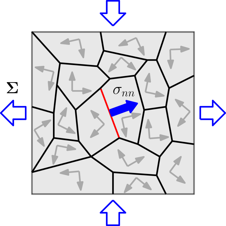
(a) polycrystalline aggregate
$(n\to\infty)$

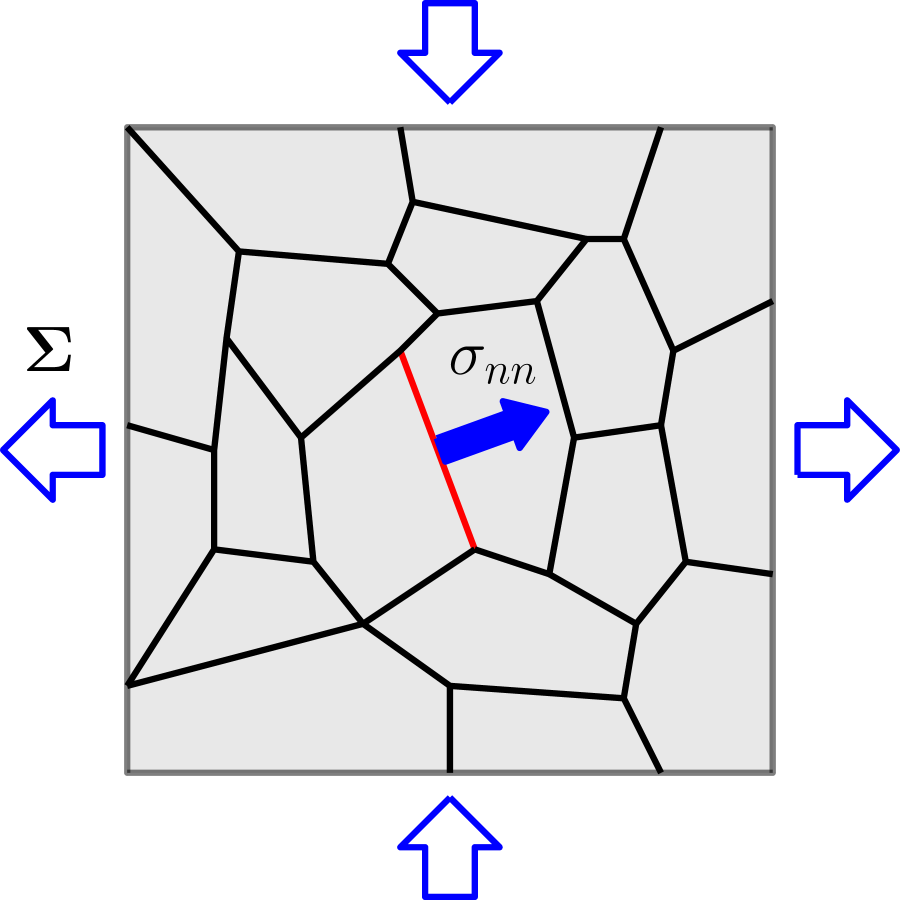
(b) isotropic case
$(n=1)$

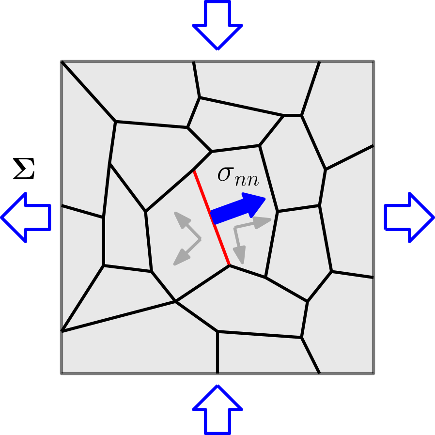
(c) bicrystal approximation
$(n=2)$

Figure 1: (a) Schematic (2D) depiction of a polycrystalline aggregate with randomly shaped crystal grains (light gray) divided by arbitrarily oriented GBs (black). The aggregate is exposed to macroscopic external loading $\mathbf{\Sigma}$ which induces a normal stress $\sigma_{nn}$ on the investigated GB (red). Crystallographic orientations of grains are indicated by local crystallographic axes (dark gray). The lowest two orders of approximation ($n=1$, $n=2$) are shown in panels (b) and (c). When no crystallographic axes are displayed, the corresponding grain is assumed isotropic (besides being homogeneous as all other grains).

Finally, the effect of neglected crystallographic orientations of all the surrounding grains, which were modelled as isotropic (the neighbourhood), is accounted for statistically as a random (Gaussian) fluctuation $\Delta\sigma_{nn}$ on top of the computed $\sigma_{nn}$. While this procedure does not produce the correct values of stresses on individual GBs, their distributions should be much more precise, allowing us to assess the likelihood of cracking initiation (though not also its exact site).

3 Isotropic approximation

At the lowest order of perturbation, all grains are initially treated as perfectly isotropic (forming a pure isotropic model), which enables us to derive analytical expressions for GB stresses. On top of these, we incorporate the statistical influence of the inherent anisotropy of the grains. Finally, we examine the impact of different materials and demonstrate how to generate material-specific estimates, particularly in relation to their elastic anisotropy. The model’s predictions are then scrutinized by comparing them to the results of numerical FE simulations, which serve as a replacement for physical experimentation and are thus meant to represent a realistic response of a perfectly elastic material under mechanical loading.

Since in isotropic approximation all the GBs are equivalent (meaning our analytical model does not distinguish between different GB types), the resulting INS distribution should correspond to that observed on randomly selected GBs in the FE simulation. For this purpose, we utilized the FE solver Abaqus [35] in the small strain regime, employing a 3D-periodic Voronoi aggregate [36, 37] with $4000$ grains and $31255$ GBs, which contain a total of $1039562$ quadratic tetrahedral finite elements (C3D10).

To facilitate a comparison with our analytical model, a weighted average of normal stresses on each GB has been produced. Henceforth, we will refer to this distribution of GB-averaged normal stresses as the reduced INS distribution. This term is used to distinguish it from the full INS distribution corresponding to normal stresses on all finite elements in the aggregate which are located on the GBs. Both distributions are weighted, either with respect to the size of GBs or the size of finite elements.

The results are presented in the following way: For the sake of demonstration, $\gamma$-Fe is consistently used in this paper as the reference material. The validity of the method is then shown for several uniform loadings $\mathbf{\Sigma}$. Only after establishing its efficacy with these loadings, the same technique is extended also to other materials. This extension includes not only cubic materials but also those with more general lattice symmetries (such as orthorhombic). Relevant properties of the chosen materials required for conducting the FE simulations can be found in Table 2 (Appendix A).

3.1 Pure isotropic model

For strictly isotropic grains, the local stress tensor $\bm{\sigma}$ is, in every point of the aggregate, equal to the external stress tensor $\mathbf{\Sigma}$. Since at any chosen GB we are interested in its component along the GB-normal direction ($\sigma_{nn}$), the stress tensor $\mathbf{\Sigma}$ must be transformed from the external loading (lab) coordinate system $(X,Y,Z)$ to a local (GB) coordinate system $(x,y,z)$:

$$\mathbf{\Sigma}^{\text{lab}} =\left(\begin{array}[]{ccc}\Sigma_{XX}&\Sigma_{XY}&\Sigma_{XZ}\\ \Sigma_{XY}&\Sigma_{YY}&\Sigma_{YZ}\\ \Sigma_{XZ}&\Sigma_{YZ}&\Sigma_{ZZ}\end{array}\right)\quad\to\quad\mathbf{\Sigma}^{\text{GB}}=\mathbf{\mathcal{R}}\,\mathbf{\Sigma}^{\text{lab}}\,\mathbf{\mathcal{R}}^{T}=\left(\begin{array}[]{ccc}\Sigma_{xx}&\Sigma_{xy}&\Sigma_{xz}\\ \Sigma_{xy}&\Sigma_{yy}&\Sigma_{yz}\\ \Sigma_{xz}&\Sigma_{yz}&\Sigma_{zz}\end{array}\right)\ ,$$ (7)

where

$$\mathbf{\mathcal{R}} =\left(\begin{array}[]{ccc}\phantom{-}\cos\theta\cos\psi\cos\phi-\sin\psi\sin\phi&\phantom{-}\cos\theta\sin\psi\cos\phi+\cos\psi\sin\phi&-\sin\theta\cos\phi\\ -\cos\theta\cos\psi\sin\phi-\sin\psi\cos\phi&-\cos\theta\sin\psi\sin\phi+\cos\psi\cos\phi&\phantom{-}\sin\theta\sin\phi\\ \sin\theta\cos\psi&\sin\theta\sin\psi&\cos\theta\\ \end{array}\right)$$ (11)

is a rotation matrix containing $3$ Euler angles ($\psi$, $\theta$, $\phi$) corresponding to a sequence of rotations ($\mathbf{\mathcal{R}_{1}}$, $\mathbf{\mathcal{R}_{2}}$, $\mathbf{\mathcal{R}_{3}}$) about $\hat{Z}$, $\mathbf{\mathcal{R}}_{1}\hat{Y}$ and $\mathbf{\mathcal{R}}_{2}\mathbf{\mathcal{R}}_{1}\hat{Z}=\hat{z}$, respectively, such that $\mathbf{\mathcal{R}}=\mathbf{\mathcal{R}_{3}}\mathbf{\mathcal{R}_{2}}\mathbf{\mathcal{R}_{1}}$, and local $z$-axis is directed along the GB normal $\hat{n}$. Consequently, the GB-normal stress

$$\begin{split}\sigma_{nn}=\Sigma_{zz}&=\left(\cos^{2}\theta\right)\,\Sigma_{ZZ}+\left(\sin^{2}\theta\,\cos^{2}\psi\right)\,\Sigma_{XX}+\left(\sin^{2}\theta\,\sin^{2}\psi\right)\,\Sigma_{YY}+\\ &+\left(\sin^{2}\theta\,\sin 2\psi\right)\,\Sigma_{XY}+\left(\sin 2\theta\,\cos\psi\right)\,\Sigma_{XZ}+\left(\sin 2\theta\,\sin\psi\right)\,\Sigma_{YZ}\end{split}$$ (12)

depends just on the polar angle $\theta$ and azimuthal angle $\psi$ (but not on the twist angle $\phi$, that is only determining the precise orientation of the local $x$ and $y$ axes). In an aggregate with randomly oriented GBs and no preferential direction, the corresponding INS distribution $\text{PDF}(\sigma_{nn})$ can be either obtained analytically or generated through Monte Carlo sampling over the uniformly distributed Euler angles $\psi$ and $\cos\theta$.

3.2 Gaussian modulation

The problem with pure isotropic model specified in Eq. (12) is that its results depend solely on the external loading $\mathbf{\Sigma}$, failing to account for the material properties. This means the model makes identical predictions for all materials, which results in significant flaws when applied to highly anisotropic materials. That is clearly visible in Fig. 2, where the resulting isotropic INS distributions (green) appear notably sharper and narrower than those generated by the FE simulations (black).

The wider and smoother FE distributions can be attributed to the fact that, in realistic aggregates, GBs are not surrounded by an isotropic medium but by specific configurations of anisotropic grains which determine the actual stress experienced at each GB site. In other words, it is the non-homogeneous nature of the neighbourhood that dictates the amount of external stress $\mathbf{\Sigma}$ that gets “transmitted” to a particular GB. Consequently, the local GB stress is not necessarily equal to $\Sigma_{zz}$, and different GBs can thus generate different responses $\sigma_{nn}$ even when they have the same orientation. As a result, realistic INS distributions tend to be wider.

This widening effect is determined by numerous independent degrees of freedom associated with the precise arrangement of grains. Their contributions to the induced GB stresses $\sigma_{nn}$ act as random fluctuations superimposed onto the estimates provided by the pure isotropic model. With the central limit theorem in mind, it is reasonable to assume that these fluctuations follow a normal distribution pattern. Written schematically:

$$\textbf{isotropic case}+\textbf{Gaussian fluctuations} \approx\textbf{INS distribution on random GBs}\ .$$ (13)

To recap, in order to mimic the effect of inhomogeneous neighbourhood surrounding each GB in anisotropic aggregate, we will model it by a Gaussian distribution ($g$) of width $\sigma_{G}$ and centered at the origin. We will also assume that this distribution has no correlation with the INS distribution generated by the pure isotropic model ($f$). As a result, the final INS distribution ($h$) will be obtained through the convolution of both distributions:

$$f(\sigma_{nn}) :=\text{PDF}(\sigma_{nn})=\frac{dP}{d\sigma_{nn}}\ ,$$ (14)

$$g(\Delta\sigma_{nn}) :=\frac{1}{\sqrt{2\pi}\,\sigma_{G}}\,e^{-\frac{1}{2}\left(\frac{\Delta\sigma_{nn}}{\sigma_{G}}\right)^{2}}\ ,$$ (15)

$$h(\sigma_{nn}) =(f\ast g)(\sigma_{nn})=\int^{\infty}_{-\infty}f(\tau)\,g(\sigma_{nn}-\tau)\,d\tau\ .$$ (16)

The $n$-th moment of the convolution is computed as

$$\mu_{h}^{(n)} =\sum_{i=0}^{n}\binom{n}{i}\mu_{f}^{(i)}\mu_{g}^{(n-i)}\ ,$$ (17)

where all the odd central moments of Gaussian distribution $g$ vanish, while for even $k$, they reduce to $\mu_{g}^{(k)}=(k-1)!!\cdot\sigma_{G}^{k}$. Since both $f$ and $g$ are also properly normalized, their zero-th moments ($\mu_{f}^{(0)}$, $\mu_{g}^{(0)}$) are equal to $1$. Hence,

$$\mu_{h}^{(1)} =\langle\sigma_{nn}\rangle_{h}=\mu_{f}^{(1)}\ ,$$ (18)

$$\mu_{h}^{(2)} =\langle(\sigma_{nn}-\langle\sigma_{nn}\rangle_{h})^{2}\rangle_{h}=\mu_{f}^{(2)}+\sigma_{G}^{2}\ ,$$ (19)

where mean value and variance of isotropic INS distribution are given by

$$\mu_{f}^{(1)} =\langle\sigma_{nn}\rangle_{f}=\frac{1}{3}\operatorname{Tr}\mathbf{\Sigma}\ ,$$ (20)

$$\mu_{f}^{(2)} =\langle(\sigma_{nn}-\langle\sigma_{nn}\rangle_{f})^{2}\rangle_{f}:=s^{2}(\sigma_{nn})=\left(\frac{2}{3\sqrt{5}}\Sigma_{\text{mis}}\right)^{2}\ .$$ (21)

Both of these expressions depend on the macroscopic loading $\mathbf{\Sigma}$ through rotational invariants ($\operatorname{Tr}{\mathbf{\Sigma}}$ or $\Sigma_{\text{mis}}$, respectively), which retain the same form in all Cartesian coordinate systems. The von Mises stress $\Sigma_{\text{mis}}$ is defined as:

$$\Sigma_{\text{mis}} :=\frac{\sqrt{3}}{\sqrt{2}}\sqrt{\operatorname{Tr}(\mathbf{\Sigma}^{2}_{\text{dev}})}\ .$$ (22)

It is related to the traceless deviatoric stress tensor

$$\mathbf{\Sigma}_{\text{dev}} :=\mathbf{\Sigma}-\tfrac{1}{3}\operatorname{Tr}(\mathbf{\Sigma})\,\mathbb{1}_{3\times 3}\ ,$$ (23)

that is typically associated with shear deformations that preserve the volume of the aggregate while changing its shape.

The same loading dependence has also been observed in FE simulations [22]. Specifically, it has been found that the first two (central) statistical moments of both the reduced and the full INS distribution are either equal to $\tfrac{1}{3}\operatorname{Tr}\mathbf{\Sigma}$ or proportional to $\Sigma_{\text{mis}}^{2}$, respectively. Identifying the convoluted distribution $h$ with $\text{PDF}(\sigma_{nn})$ obtained from the FE simulation not only implies that $\sigma_{G}$ should also scale with $\Sigma_{\text{mis}}$, but it also allows us to use Eq. (19) to determine the value of $\sigma_{G}$.

Finally, the modelling approach is validated in Fig. 2, where the computed $\sigma_{G}$ is utilized to generate the convoluted distributions $h$ (red) for several different uniform loadings $\mathbf{\Sigma}^{\text{lab}}$ (but here showing only three such examples) and then compare them to the (reduced) distributions of GB stresses from FE simulations (black).

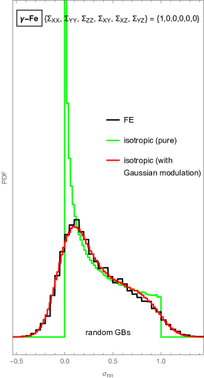
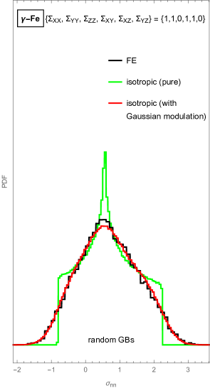
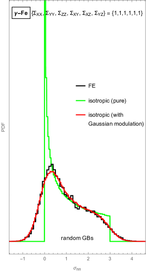
Figure 2: Reduced INS distributions for $\gamma$-Fe and three uniform loadings. Comparison of FE results (black; $N=31255$) and estimates from the analytical isotropic model without (green) and with Gaussian fluctuations (red; $\sigma_{G}^{(1)}=0.136\times\Sigma_{\text{mis}}$).

Another factor contributing to the widening of INS distributions in realistic (FE) scenarios is the variation of induced stress across the GB, in contrast to the constant stress assumed in our simplified model. To account for this behaviour and thus describe the full INS distribution (instead of just the reduced version), we can perform one more convolution with additional Gaussian (characterized by a different width $\sigma_{G}^{(2)}$). Since the convolution of two Gaussian distributions results in another Gaussian distribution whose variance is the sum of variances of the original distributions, this procedure is equivalent to a single convolution with a Gaussian of width:

$$\sigma_{G}=\sqrt{(\sigma_{G}^{(1)})^{2}+(\sigma_{G}^{(2)})^{2}}\ .$$ (24)

Henceforth we will denote the width of the Gaussian distribution in the reduced case as $\sigma_{G}^{(1)}$ and the width in the full case as $\sigma_{G}$. The effect of this additional convolution with a normal distribution of width $\sigma_{G}^{(2)}$ on the shape of the INS distribution is depicted in Fig. 3.

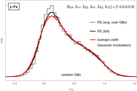
Figure 3: A comparison between the modelled (red; $\sigma_{G}=0.167\times\Sigma_{\text{mis}}$) and realistic (black; $N=3105904$) full INS distribution for $\gamma$-Fe and uniaxial tensile loading. The reduced INS distribution (gray; $N=31255$) is also shown for comparison. Both FE distributions are almost identical due to a relatively modest widening needed to correct for the averaging of stresses over the GBs; $(\sigma_{G}^{(2)})^{2}\ll(\sigma_{G}^{(1)})^{2}$.

3.3 Effect of the material

The same procedure can be performed also for other materials. Because the predictions of the pure isotropic model are material-independent, the differences in INS distributions for various materials have to emerge at the convolution level (owing to distinct, material-specific widths of Gaussian distributions). In other words, material properties affect only the width of the fluctuations. Therefore, $\sigma_{G}$ is also the only parameter that needs adaptation in our analytical description.

Most significant is its correlation with the material’s anisotropy. While there should be no fluctuations in the isotropic case (meaning the Gaussian is infinitely narrow), $\sigma_{G}$ is expected to increase with the growing anisotropy of the material. As a measure of material anisotropy, we utilize the universal elastic anisotropy index $A^{u}$ [38] since it is applicable to any lattice symmetry (not only cubic). By matching the width of a (full) INS distribution produced in FE simulation, $\sigma_{G}$ can be calculated for any material and then shown as a function of its $A^{u}$, see Fig. 4.

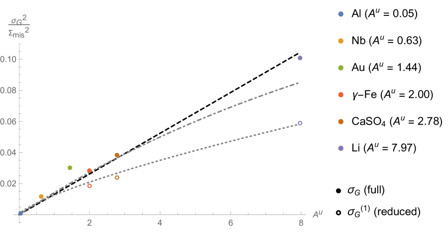
Figure 4: To simulate the response of anisotropic materials to external loading, normally distributed random fluctuations are added to the GB-normal stresses induced in isotropic crystal. The width $\sigma_{G}$ of the fluctuation distribution is determined by matching the standard deviation of FE distribution. The square of this width is shown as a function of the universal elastic anisotropy index $A^{u}$ for several materials. Additionally, a linear fit (black dashed line) is depicted, while the gray dash-dotted curve represents the fit from Eq. (26). For comparison, a $\sigma_{G}^{(1)}$ fit [22] (gray dotted curve) is also included, demonstrating that the predominant widening effect arises from the anisotropic neighbourhood of the GB, rather than from the averaging of stresses over each GB (i.e., $\sigma_{G}^{(1)}>\sigma_{G}^{(2)}$).

The observed pattern is reasonably well-fitted by the linear dependence

$$\sigma_{G}^{2} =k\,A^{u}\ ,$$ (25)

which appropriately approaches zero in the isotropic limit ($A^{u}=0$). The current best estimate for the proportionality factor is $k=0.013$. In the past, an approximate relation between the standard deviation of the INS distribution on random GBs and the material’s anisotropy was proposed for uniaxial loading [39]:

$$s_{FE}\left(\frac{\sigma_{nn}}{\Sigma}\right) \approx\frac{4}{3\sqrt{5}}\,\frac{A^{u}+6}{A^{u}+12}\ .$$ (26)

However, this relation tends to undershoot the true values of $s_{FE}(\sigma_{nn})$, especially for large $A^{u}$. As a result, the approximation $(\frac{2}{3\sqrt{5}})^{2}+\sigma_{G}^{2}=\left(\frac{4}{3\sqrt{5}}\,\frac{A^{u}+6}{A^{u}+12}\right)^{2}$ also underestimates the size of Gaussian fluctuations $\sigma_{G}$ for materials with larger anisotropy, as shown by the gray dash-dotted curve in Fig. 4.

A comparison between the modelled INS distributions (with $\sigma_{G}$ determined from the linear fit in Eq. (25)) and those obtained numerically is presented in Fig. 5. A (fairly) good agreement between both can be observed.

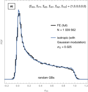
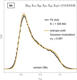
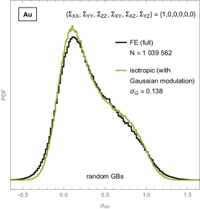
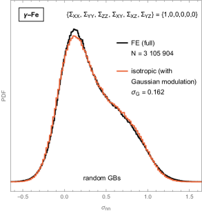
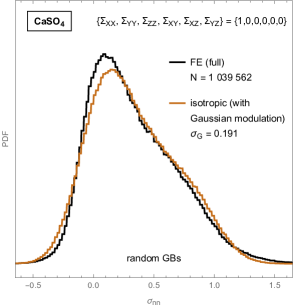
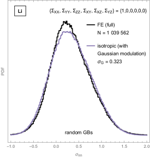
Figure 5: INS distributions induced by uniaxial tensile loading for various selected materials. A comparison is shown between the results of numerical simulation and an isotropic model convoluted with a Gaussian distribution. The value of its width $\sigma_{G}$ was determined from the linear fit shown in Fig. 4. The number of finite elements in the aggregate is denoted by $N$. For $\gamma$-Fe, the data from three different Voronoi aggregates has been combined, which effectively corresponds to using a single aggregate with $12000$ grains.

The reliability of the isotropic approximation for GB-normal stresses on random GBs is further illustrated in Fig. 6. As observed in its left panels, the average value of $\sigma_{nn}$ at GBs with the same inclination (denoted by $\langle\sigma_{nn}\rangle_{\theta}$) closely aligns with the prediction of the pure isotropic model. Additionally, the stress fluctuation around $\langle\sigma_{nn}\rangle_{\theta}$ is accurately captured by a Gaussian distribution, with a width that remains almost constant across different inclinations. The validity of these observations holds true irrespective of whether we consider the reduced or full INS distributions. The only difference is that the Gaussian is wider in the latter case, as explained in Footnote 5. For crystal lattices with non-cubic symmetry, the average value of $\sigma_{nn}$ at a chosen inclination is still predicted by the isotropic model, but the stresses no longer appear to be normally distributed around this value. Instead, their distribution appears slightly asymmetric.

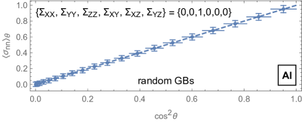
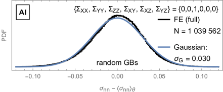
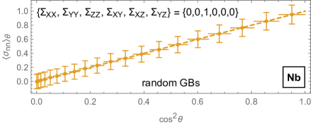
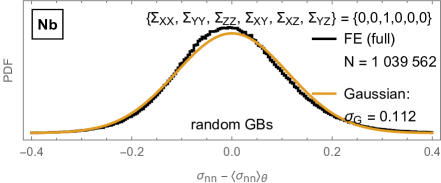
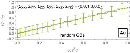
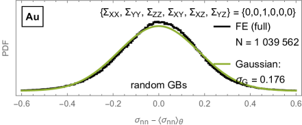
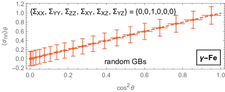
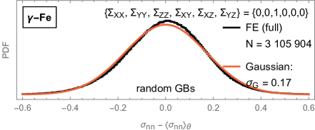
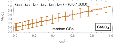
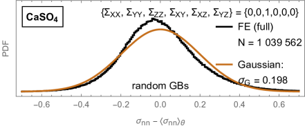
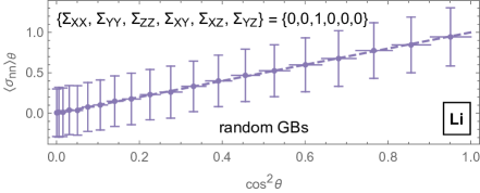
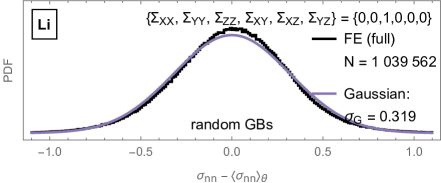
Figure 6: Left panels: The value of $\sigma_{nn}$ averaged over all (random) GBs in the aggregate with the same inclination $\theta$ relative to uniaxial external loading. Horizontal lines indicate the width of the bin $\cos\theta\pm 0.025$, while vertical bars correspond to the standard deviation of the $\sigma_{nn}$ distribution in each bin (which appears to be practically independent of $\theta$). The dashed line represents the value for a perfectly isotropic material ($\sigma_{nn}=\Sigma_{zz}=\cos^{2}\theta$). Right panels: The distribution of normal stresses around the values predicted by the pure isotropic model. Except for CaSO₄, it is very well-described by a Gaussian of width $\sigma_{G}$ (whose value was fitted rather than determined by the linear approximation shown in Fig. 4).

In conclusion, the presented isotropic model contains a single free parameter $k$ requiring fitting, and yet manages to successfully predict the INS distributions on random GBs for any chosen material and uniform external loading. However, this is still not sufficient for accurately estimating the likelihood of intergranular cracking initiation, as different GBs possess distinct thresholds for cracking. To achieve that goal, one is forced to go beyond the isotropic approximation and consider the INS distributions on individual GB types.

4 Bicrystal model

Each GB type is characterized by a relationship between the GB plane and the orientations of the crystal lattices on either side of it. The GB orientation is specified by its normal vector, which contributes two degrees of freedom in each of the two crystallographic systems (being expressed in them as unit-length vectors $(a,b,c)$ and $(d,e,f)$, respectively), while a relative rotation about the GB normal between both crystallographic systems introduces another parameter, known as the twist angle ($\Delta\omega$). Alternatively, three degrees of freedom are required to relate the crystallographic systems of both adjacent grains, and an additional two degrees to specify the GB plane in one of them, again resulting in a total of five degrees of freedom to determine the GB type.

To investigate the INS distribution across all GBs of a particular $[abc]$-$[def]$-$\Delta\omega$ type, one would require either a considerably large random aggregate (with crystallographic orientation of each grain and normal direction of every GB randomly assigned) to accumulate sufficient statistics, or a dedicated aggregate in which the number of GBs of that type is increased by design. We opted for the latter approach and thus created a distinct aggregate for each studied GB type. These aggregates share the same grain topology and FE-mesh structure, and differ only in the crystallographic orientations of the grains. However, due to topological constraints, only a limited subset of all GBs in them can be assigned a special character.

To enhance the statistical significance of our results, a selected GB type was imposed on the largest available GBs in the aggregate — those with the largest area, which also typically contain the highest number of finite elements. In our case, featuring an aggregate with $4000$ grains and a total of $31255$ GBs, only $N=1636$ GBs (representing approximately $17\%$ of the entire GB area and containing $159461$ finite elements) correspond to the designated GB type. As a result, the accuracy of our numerical results is noticeably worse than in the isotropic approximation, where all GBs could be included in the analysis. Consequently, the FE distributions presented for individual GB types are less refined.

In this section, we begin by presenting the empirical findings from our previous numerical studies [32, 22]. Then the (pure) bicrystal analytical model is introduced along with its general solution. Finally, the model predictions are assessed through a comparison with the FE results. Similar to the isotropic model, Gaussian modulation is introduced to improve the INS distributions. However, unlike in the isotropic scenario, a single parameter ($\sigma_{G}$) is not sufficient to accurately describe the INS distribution across the GBs of a specific type. The reason behind this lies in the fact that the standard deviation of its pure bicrystal-model estimate can exceed the FE value if all grains are assumed to have average, aggregate-scale (bulk) elastic properties (despite such assumption manages to correctly reproduce the distribution’s mean value). Hence, we introduce two additional parameters, $\alpha$ and $\beta$, which are related to the stiffness of the GB. All three parameters ($\alpha$, $\beta$, and $\sigma_{G}$) are allowed to vary as functions of both the GB type and material properties.

While we have successfully found a simple phenomenological relation that links $\alpha$ and $\beta$ with $E_{12}$, this proves more difficult for $\sigma_{G}$ due to its sensitivity to uncertainties arising from finite aggregate size in numerical simulations. Consequently, expressing these parameters as functions of material properties, akin to the linear fit in the isotropic case, is even more challenging. Improving upon the proposed fits would thus require a substantial increase in the amount of numerical data. Nevertheless, our existing fits demonstrate a robust ability to predict INS distributions across a wide range of materials and GB types.

4.1 Review of numerical simulation results

Below, the most important insights from our previous FE study [32] of selected materials with cubic crystal lattices are gathered:

1. twist-angle (in)dependence of $\text{PDF}(\sigma_{nn})$:
   The results for $\langle abc\rangle$-$twist$ GBs suggested that the first two statistical moments of INS distributions remain virtually unaffected by the twist angle $\Delta\omega$ between both grains (although its value might still affect the corresponding GB strength). However, later research [22] has revealed that while this observation holds for $\langle\sigma_{nn}\rangle$ of $[abc]$-$[def]$-$\Delta\omega$ GB types, it is no longer true for their $s(\sigma_{nn})$. Nonetheless, we consider this effect to be a higher-order correction. As a result, the value of $\Delta\omega$ can be assigned at random for each GB in numerical simulations, and $4$ degrees of freedom effectively suffice to specify a GB type in relation to the local GB stress. In our discussions, we colloquially refer to it as the $[abc]$-$[def]$ GB type.

2. universal value of $\langle\sigma_{nn}\rangle$:
   INS distributions have a universal mean value for every GB type and in any material with cubic lattice symmetry:

   $$\langle\sigma_{nn}\rangle =\frac{1}{3}\operatorname{Tr}{\mathbf{\Sigma}}\ .$$ (27)

   Consequently, the proportion of GBs of a particular type with stresses exceeding the threshold value is, in the first approximation, well characterized by the standard deviation of the corresponding INS distribution.

3. relevance of effective GB-stiffness parameter for $s(\sigma_{nn})$:
   The effective GB stiffness $E_{12}$ has been identified as the sole parameter needed to relate the GB type to the standard deviation of the corresponding INS distribution. An approximate phenomenological expression has been proposed

   $$\begin{split}s(\sigma_{nn};E_{12},A,\mathbf{\Sigma})&:=\sqrt{\langle(\sigma_{nn}-\langle\sigma_{nn}\rangle)^{2}\rangle}\\ &\approx A_{1}(A)\arctan{\left(A_{2}(A)\,E_{12}^{A_{3}(A)}\right)}\,\Sigma_{\text{mis}}\ ,\end{split}$$ (28)

   where $A_{1}$, $A_{2}$ and $A_{3}$ are material-specific fitting coefficients, and

   $$A =\frac{2(s_{11}-s_{12})}{s_{44}}\ ,$$ (29)

   $$E_{12} =\frac{2\hskip 1.00006pt\hbox{\vbox{\hrule height=0.5pt\kern 1.72218pt\hbox{\kern-1.00006pt$E$\kern-1.00006pt}}}\hskip 1.00006pt^{-1}}{E_{abc}^{-1}+E_{def}^{-1}}$$ (30)

   represent the Zener elastic anisotropy index [40], and the effective GB stiffness, while

   $$E_{hkl}^{-1} =s_{11}-2s_{0}\frac{(hk)^{2}+(hl)^{2}+(kl)^{2}}{(h^{2}+k^{2}+l^{2})^{2}}\ ,$$ (31)

   $$s_{0} :=s_{11}-s_{12}-\frac{s_{44}}{2}=\frac{s_{44}}{2}(A-1)$$ (32)

   are the inverse Young’s modulus of a grain along the $(h,k,l)$-direction, and a specific combination of the eigenbasis components ($s_{11}$, $s_{12}$, and $s_{44}$) of the compliance tensor in Voigt notation, which vanishes for isotropic materials (i.e., $s_{0}=0$ for $A=1$).

   The parameter    $E$   denotes the average (bulk) Young’s modulus of the aggregate, given by

    $$E =\frac{9KG}{3K+G}\ ,$$ (33)

   where compression ($K$) and shear ($G$) elastic moduli can be estimated using a self-consistent approach [41]. For crystal grains with cubic lattice symmetry, assembled in a random (macroscopically isotropic) aggregate, these expressions simplify to the following forms [42]:

   $$K =\frac{1}{3(s_{11}+2s_{12})}\ ,$$ (34)

   $$G =\left\{\begin{array}[]{c}\!\!8\,(s_{11}\!+\!2s_{12})(s_{11}\!-\!s_{12})\,s_{44}\,G^{3}+(5s_{11}\!+\!s_{12})\,s_{44}\,G^{2}-(7s_{11}\!+\!11s_{12})\,G=1\\ G>0\end{array}\right.\!\!.$$ (37)

In summary, out of the five degrees of freedom specifying a $[abc]$-$[def]$-$\Delta\omega$ GB type, only one particular combination of $a$, $b$, $c$, $d$, $e$, and $f$ — namely, the $E_{12}$ — is needed to determine the local stress distribution. Since $E_{12}$ can be considered essentially a “bicrystal” quantity (depending only on the properties of the two nearest neighbours), the above observations (based on “realistic” simulations that properly take into account all the grains in the aggregate, not just the closest two) suggest that there is no need to go beyond the second-order approximation (the bicrystal model) for the intended estimates of GB-stress distributions.

One of the primary objectives of this paper is thus to elucidate these observations and to derive them within a simplified framework based on the bicrystal approximation. Especially relevant in this context is recognizing the effective stiffness of the bicrystal pair along the GB-normal direction ($E_{12}$) and the Zener anisotropy index ($A$) as key parameters. It’s worth noting that material properties are contained not only in $A$ but also in $E_{12}$. Its value implicitly depends on $s_{ij}$ and thus the choice of material; cf. Eqs. (30)–(37). The combined effect of material-dependent parameters $A$ and $E_{12}$ is illustrated in Fig. 7.

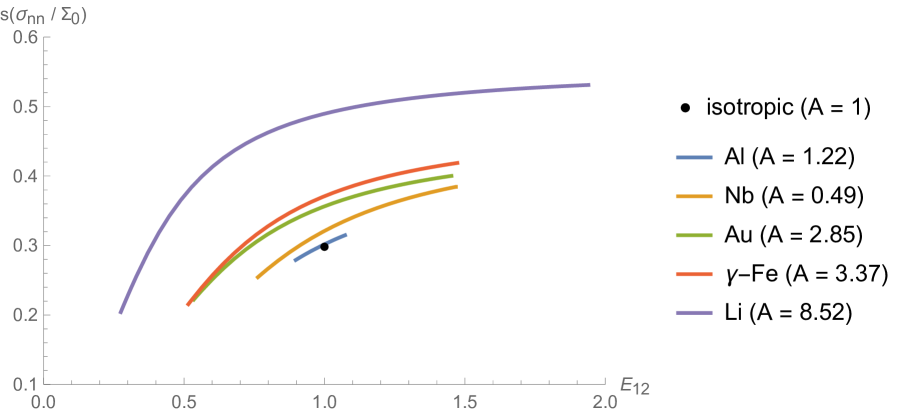
Figure 7: Standard deviation $s(\sigma_{nn}/\Sigma_{0})$ as a function of GB stiffness $E_{12}$ for uniaxial external loading of magnitude $\Sigma_{0}$; showing its fit specified in Eq. (63). Several (cubic) materials are presented, arranged in increasing order of anisotropy (specified as a deviation from the isotropic case, also provided for reference). The indicated values of Zener index $A$ uniquely determine the corresponding fitting coefficients $A_{k}$. The values on the vertical axis correspond to the full INS distributions obtained from all finite elements within the aggregate that belong to GBs of a specific type. The same fitting function (albeit with different coefficients $A_{k}$) could also be applied to the narrower reduced INS distributions (see Fig. 8).

4.2 The model

We wish to obtain a component of stress tensor along the GB-normal direction ($\sigma_{nn}$) for any chosen GB in the aggregate that is subjected to a macroscopic external loading $\mathbf{\Sigma}$. To achieve this, a generalized Hooke’s law:

$$\epsilon_{ij}^{(N)} =\sum_{k,l=1}^{3}\tilde{s}_{ijkl}^{(N)}\,\sigma_{kl}^{(N)}\ ,\quad i,j=1,2,3\ ,$$ (38)

relating the components of local strain ($\epsilon_{ij}$), compliance ($\tilde{s}_{ijkl}$) and stress ($\sigma_{ij}$) tensors, or its inverse containing the elastic stiffness tensor ($\tilde{C}_{ijkl}$):

$$\sigma_{ij}^{(N)} =\sum_{k,l=1}^{3}\tilde{C}_{ijkl}^{(N)}\,\epsilon_{kl}^{(N)}\ ,\quad i,j=1,2,3\ ,$$ (39)

needs to be solved for a pair of grains ($N=1,2$) enclosing the investigated GB from both sides. Depending on the position of the GB within the aggregate, the grains may be of various shapes and sizes, and their crystal lattices can posses arbitrary orientations in relation to external loading. The GB itself can also be oriented in any direction (uncorrelated with the crystallographic orientations of both surrounding grains).

The simplest scenario considers the grains with cubic lattice symmetry. In such case, the components of the $rank$-$4$ compliance tensor $\tilde{s}_{ijkl}$ (or elasticity tensor $\tilde{C}_{ijkl}$) depend on just three material parameters ($s_{11}$, $s_{12}$ and $s_{44}$), and many of the relations simplify substantially. When expressed in a local (grain) coordinate system $(n_{1},n_{2},n_{3})$ aligned with the crystallographic axes of the underlying lattice, the tensor assumes the following form:

$$\begin{split}s_{mmmm}&:=s_{11}\ ,\quad m=1,2,3\ ,\\ s_{mnmn}=s_{mnnm}&:=\frac{s_{44}}{4}\ ,\quad m,n\neq m=1,2,3\ ,\\ s_{mmnn}&:=s_{12}\ ,\quad m,n\neq m=1,2,3\ ,\\ s_{mnop}&:=0\ ,\quad\text{otherwise}\ ,\end{split}$$ (40)

and similarly for the stiffness tensor:

$$\begin{split}C_{mmmm}&:=C_{11}\ ,\quad m=1,2,3\ ,\\ C_{mnmn}=C_{mnnm}&:=C_{44}\ ,\quad m,n\neq m=1,2,3\ ,\\ C_{mmnn}&:=C_{12}\ ,\quad m,n\neq m=1,2,3\ ,\\ C_{mnop}&:=0\ ,\quad\text{otherwise}\ ,\end{split}$$ (41)

where the transformation rules between both

$$\begin{split}s_{11}&=\frac{C_{11}+C_{12}}{(C_{11}-C_{12})(C_{11}+2C_{12})}\ ,\\ s_{12}&=-\frac{C_{12}}{(C_{11}-C_{12})(C_{11}+2C_{12})}\ ,\\ s_{44}&=\frac{1}{C_{44}}\ ,\\ s_{0}&=\frac{1}{C_{11}-C_{12}}-\frac{1}{2C_{44}}\end{split}$$ (42)

are symmetric to $s_{ij}\leftrightarrow C_{ij}$.

But for our purposes, it is more convenient to express all the quantities in a local (GB) coordinate system $(x,y,z)$, in which the $z$-axis is aligned with the GB normal. The transformations

$$\begin{split}\tilde{s}_{ijkl}^{(N)}&=\sum_{m,n,o,p=1}^{3}R_{im}^{(N)}R_{jn}^{(N)}R_{ko}^{(N)}R_{lp}^{(N)}\,s_{mnop}\\ &=\left(\sum_{m=1}^{3}R_{im}^{(N)}R_{jm}^{(N)}R_{km}^{(N)}R_{lm}^{(N)}\right)s_{0}+(\delta_{ij}\delta_{kl})\,s_{12}+(\delta_{ik}\delta_{jl}+\delta_{il}\delta_{jk})\,\frac{s_{44}}{4}\ ,\end{split}$$ (43)

$$\begin{split}\tilde{C}_{ijkl}^{(N)}&=\sum_{m,n,o,p=1}^{3}R_{im}^{(N)}R_{jn}^{(N)}R_{ko}^{(N)}R_{lp}^{(N)}\,C_{mnop}\\ &=\left(\sum_{m=1}^{3}R_{im}^{(N)}R_{jm}^{(N)}R_{km}^{(N)}R_{lm}^{(N)}\right)(C_{11}\!-\!C_{12}\!-\!2\,C_{44})+(\delta_{ij}\delta_{kl})\,C_{12}+(\delta_{ik}\delta_{jl}\!+\!\delta_{il}\delta_{jk})\,C_{44}\end{split}$$ (44)

involve the (orthogonal) rotation matrix

$$\mathbf{R} =\left(\begin{array}[]{ccc}\phantom{-}\frac{hl\cos\omega}{\sqrt{h^{2}+k^{2}}\sqrt{h^{2}+k^{2}+l^{2}}}-\frac{k\sin\omega}{\sqrt{h^{2}+k^{2}}}&\phantom{-}\frac{kl\cos\omega}{\sqrt{h^{2}+k^{2}}\sqrt{h^{2}+k^{2}+l^{2}}}+\frac{h\sin\omega}{\sqrt{h^{2}+k^{2}}}&-\frac{\sqrt{h^{2}+k^{2}}\cos\omega}{\sqrt{h^{2}+k^{2}+l^{2}}}\\ -\frac{hl\sin\omega}{\sqrt{h^{2}+k^{2}}\sqrt{h^{2}+k^{2}+l^{2}}}-\frac{k\cos\omega}{\sqrt{h^{2}+k^{2}}}&-\frac{kl\sin\omega}{\sqrt{h^{2}+k^{2}}\sqrt{h^{2}+k^{2}+l^{2}}}+\frac{h\cos\omega}{\sqrt{h^{2}+k^{2}}}&\phantom{-}\frac{\sqrt{h^{2}+k^{2}}\sin\omega}{\sqrt{h^{2}+k^{2}+l^{2}}}\\ \frac{h}{\sqrt{h^{2}+k^{2}+l^{2}}}&\frac{k}{\sqrt{h^{2}+k^{2}+l^{2}}}&\frac{l}{\sqrt{h^{2}+k^{2}+l^{2}}}\end{array}\right)\ ,$$ (48)

with $(h,k,l)$ representing the direction of the GB normal expressed in the grain system $(n_{1},n_{2},n_{3})$, and $\omega$ the angle of rotation (twist) about the GB normal. Two such matrices $\mathbf{R}^{(N)}$ are needed for every GB (one for each grain), with parameters $(a,b,c)$ and $\omega_{1}$ used for the first grain ($N=1$) and $(d,e,f)$ and $\omega_{2}$ for the second grain ($N=2$). Their numerical values determine the corresponding GB type $[abc]$-$[def]$-$\Delta\omega$.

The transformation of the macroscopic loading from the lab coordinate system $(X,Y,Z)$ to the GB coordinate system $(x,y,z)$ is carried out in the same manner as before, cf. Eqs. (7)–(11). The expressions for the external stress tensor components in the GB coordinate system can be found in Appendix B.

Since strain ($\epsilon_{ij}$) and stress ($\sigma_{ij}$) are both represented by symmetric tensors, Eq. (38) yields $6$ constitutive equations for each grain, and thus $12$ altogether. To solve them, a matching number of boundary conditions is needed. We will categorize them into $6$ “inner” and $6$ “outer” conditions, depending on whether they apply to the grain boundary or to the bicrystal pair. The inner conditions are:

1. stress continuity across the GB

   $$\sigma_{xz}^{(1)}=\sigma_{xz}^{(2)}\quad,\quad\sigma_{yz}^{(1)}=\sigma_{yz}^{(2)}\quad,\quad\sigma_{zz}^{(1)}=\sigma_{zz}^{(2)}\ ,$$ (49)

2. strain compatibility across the GB

   $$\epsilon_{xx}^{(1)}=\epsilon_{xx}^{(2)}\quad,\quad\epsilon_{xy}^{(1)}=\epsilon_{xy}^{(2)}\quad,\quad\epsilon_{yy}^{(1)}=\epsilon_{yy}^{(2)}\ ,$$ (50)

while the outer conditions are specifying how the investigated pair of grains is deformed as a whole when a specific macroscopic external loading $\mathbf{\Sigma}$ is applied to the aggregate:

$$\begin{split}V_{1}\,\epsilon_{xx}^{(1)}+V_{2}\,\epsilon_{xx}^{(2)}=(V_{1}+V_{2})\,\hskip 1.00006pt\hbox{\vbox{\hrule height=0.5pt\kern 1.72218pt\hbox{\kern-1.00006pt$\epsilon$\kern-1.00006pt}}}\hskip 1.00006pt^{b}_{xx}\quad,\quad V_{1}\,\epsilon_{yz}^{(1)}+V_{2}\,\epsilon_{yz}^{(2)}=(V_{1}+V_{2})\,\hskip 1.00006pt\hbox{\vbox{\hrule height=0.5pt\kern 1.72218pt\hbox{\kern-1.00006pt$\epsilon$\kern-1.00006pt}}}\hskip 1.00006pt^{b}_{yz}\ ,\\ V_{1}\,\epsilon_{yy}^{(1)}+V_{2}\,\epsilon_{yy}^{(2)}=(V_{1}+V_{2})\,\hskip 1.00006pt\hbox{\vbox{\hrule height=0.5pt\kern 1.72218pt\hbox{\kern-1.00006pt$\epsilon$\kern-1.00006pt}}}\hskip 1.00006pt^{b}_{yy}\quad,\quad V_{1}\,\epsilon_{xz}^{(1)}+V_{2}\,\epsilon_{xz}^{(2)}=(V_{1}+V_{2})\,\hskip 1.00006pt\hbox{\vbox{\hrule height=0.5pt\kern 1.72218pt\hbox{\kern-1.00006pt$\epsilon$\kern-1.00006pt}}}\hskip 1.00006pt^{b}_{xz}\ ,\\ V_{1}\,\epsilon_{zz}^{(1)}+V_{2}\,\epsilon_{zz}^{(2)}=(V_{1}+V_{2})\,\hskip 1.00006pt\hbox{\vbox{\hrule height=0.5pt\kern 1.72218pt\hbox{\kern-1.00006pt$\epsilon$\kern-1.00006pt}}}\hskip 1.00006pt^{b}_{zz}\quad,\quad V_{1}\,\epsilon_{xy}^{(1)}+V_{2}\,\epsilon_{xy}^{(2)}=(V_{1}+V_{2})\,\hskip 1.00006pt\hbox{\vbox{\hrule height=0.5pt\kern 1.72218pt\hbox{\kern-1.00006pt$\epsilon$\kern-1.00006pt}}}\hskip 1.00006pt^{b}_{xy}\ .\end{split}$$ (51)

If the average strain of the bicrystal $\hskip 1.00006pt\hbox{\vbox{\hrule height=0.5pt\kern 1.72218pt\hbox{\kern-1.00006pt$\epsilon$\kern-1.00006pt}}}\hskip 1.00006pt^{b}_{ij}$ and the volumes of the corresponding grains, $V_{1}$ and $V_{2}$, were known for every pair of grains, the equations (38) and (49)–(51) would yield an exact solution for $\sigma_{nn}:=\sigma_{zz}^{(1)}=\sigma_{zz}^{(2)}$ at each GB (neglecting that, in practice, strain and stress are not constant throughout the grains). However, obtaining the correct values of $\hskip 1.00006pt\hbox{\vbox{\hrule height=0.5pt\kern 1.72218pt\hbox{\kern-1.00006pt$\epsilon$\kern-1.00006pt}}}\hskip 1.00006pt^{b}_{ij}$ requires solving the equations for all the grains in the aggregate simultaneously, which is feasible only numerically, e.g., by relying on the finite element method. Such approach is both computationally demanding and time-consuming due to the large number of grains involved. It is also impractical since it requires the knowledge of the exact configuration of all the grains in the aggregate.

Another way to address the problem is to make some reasonable assumptions about the deformation of the bicrystal pair (i.e., the outer boundary conditions), and try to solve the model analytically. Several factors contribute to the GB stress. Ranked in decreasing order of importance, the most relevant are: GB orientation, GB type, and the neighbourhood consisting of all the grains surrounding the bicrystal pair. As previously explained, in this study we adopted a perturbative approach, approximating the neighbourhood with a homogeneous and isotropic matrix material (into which the bicrystal pair is embedded). This allows us to consider only a single pair of grains rather than the entire aggregate, and to derive a solution of the bicrystal-model equations for any GB (specified by its orientation and the corresponding GB type).

The simplest assumption that can be made about $\hskip 1.00006pt\hbox{\vbox{\hrule height=0.5pt\kern 1.72218pt\hbox{\kern-1.00006pt$\epsilon$\kern-1.00006pt}}}\hskip 1.00006pt^{b}_{ij}$ is to use the average strain approximation

$$\hskip 1.00006pt\hbox{\vbox{\hrule height=0.5pt\kern 1.72218pt\hbox{\kern-1.00006pt$\epsilon$\kern-1.00006pt}}}\hskip 1.00006pt^{b}_{ij}=\hskip 1.00006pt\hbox{\vbox{\hrule height=0.5pt\kern 1.72218pt\hbox{\kern-1.00006pt$\epsilon$\kern-1.00006pt}}}\hskip 1.00006pt_{ij} =\frac{1+\hskip 1.00006pt\hbox{\vbox{\hrule height=0.5pt\kern 1.72218pt\hbox{\kern-1.00006pt$\nu$\kern-1.00006pt}}}\hskip 1.00006pt}{\hskip 1.00006pt\hbox{\vbox{\hrule height=0.5pt\kern 1.72218pt\hbox{\kern-1.00006pt$E$\kern-1.00006pt}}}\hskip 1.00006pt}\Sigma_{ij}-\frac{\hskip 1.00006pt\hbox{\vbox{\hrule height=0.5pt\kern 1.72218pt\hbox{\kern-1.00006pt$\nu$\kern-1.00006pt}}}\hskip 1.00006pt}{\hskip 1.00006pt\hbox{\vbox{\hrule height=0.5pt\kern 1.72218pt\hbox{\kern-1.00006pt$E$\kern-1.00006pt}}}\hskip 1.00006pt}(\operatorname{Tr}\mathbf{\Sigma})\,\delta_{ij}\ ,$$ (52)

where

 $$\nu =\frac{3K-2G}{2(3K+G)}=\frac{1}{2}\left(1-\hskip 1.00006pt\hbox{\vbox{\hrule height=0.5pt\kern 1.72218pt\hbox{\kern-1.00006pt$E$\kern-1.00006pt}}}\hskip 1.00006pt\,(s_{11}+2s_{12})\right)$$ (53)

is the average Poisson’s ratio of the material (and last equality applies only to the cubic lattice symmetry). The problem with this ansatz is that it produces an incorrect response — the magnitude of induced stress $\sigma_{nn}$ is too large for very stiff GBs (as they should not deform as much as the bulk material) and too small for very soft GBs (which should deform more than the bulk). This can be observed in Fig. 8, showing a comparison between the results of FE simulation and the bicrystal model. Both exhibit similar trends for the “width” of INS distribution as a function of stiffness of the corresponding GB type, but having different slopes. The realistic (FE) curve is less steep since for soft GBs (small $E_{12}$) both tensile and compressive strains are larger than the average strain of the aggregate ($\hskip 1.00006pt\hbox{\vbox{\hrule height=0.5pt\kern 1.72218pt\hbox{\kern-1.00006pt$\epsilon$\kern-1.00006pt}}}\hskip 1.00006pt_{ij}$) and thus the magnitude of stress bigger than the bicrystal estimate based on Eq. (52). The standard deviation is thus underestimated in the bicrystal model. Conversely, for stiff GBs (large $E_{12}$), the bicrystal-model estimate surpasses the true standard deviation.

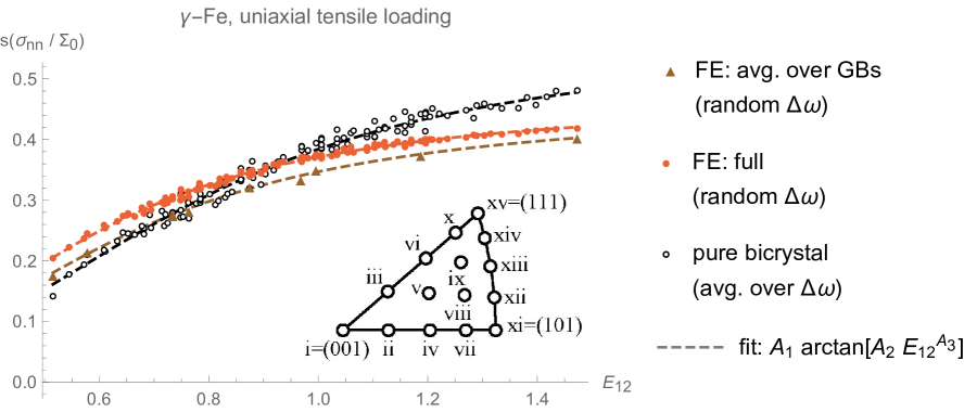
Figure 8: Standard deviation $s(\sigma_{nn}/\Sigma_{0})$ as a function of GB stiffness $E_{12}$ for $\gamma$-Fe and uniaxial loading of strength $\Sigma_{0}$. Comparison is made between the results of FE simulation and the solution of a simplified bicrystal model. The $120$ dots in each case correspond to selecting GB normals $(a,b,c)$ and $(d,e,f)$ among the $15$ predefined directions from the standard stereographic triangle shown in the inset. In addition to the full distribution, we also display the reduced distribution (denoted by triangles). The same fitting function (63), albeit with different coefficients $A_{k}$, was used in all three cases.

Different points in Fig. 8 represent different $[abc]$-$[def]$ GB types obtained by selecting GB normals $(a,b,c)$ and $(d,e,f)$ from the $15$ directions within the standard stereographic triangle: $i=[001]$, $ii=[104]$, $iii=[114]$, $iv=[102]$, $v=[214]$, $vi=[112]$, $vii=[304]$, $viii=[314]$, $ix=[324]$, $x=[334]$, $xi=[101]$, $xii=[414]$, $xiii=[212]$, $xiv=[434]$ and $xv=[111]$. Note that some of the GB types correspond to the same value of $E_{12}$ because the Young’s moduli along different directions can be the same (specifically, $E_{hkl}^{-1}=s_{11}-s_{0}/2$ along the $[101]$, $[112]$ and $[314]$ directions). For each GB type, the $\sigma_{nn}$ distribution (originating mainly from random orientations of GBs rather than from their different neighbourhoods) is obtained in FE simulation. Its standard deviation (representing the “width” of the distribution) is shown on the vertical axis of Fig. 8.

To obtain $\sigma_{nn}$ in the bicrystal case, Eq. (38) along with boundary conditions (49)–(51), and imposing the approximation (52), needs to be solved for a specific GB orientation and GB type. Here, this was done numerically, and thus material properties, loading conditions and the relative sizes of both grains had to be specified. INS distribution for a chosen GB type is then produced by performing a Monte Carlo (MC) sampling over the uniformly distributed parameters $\psi$, $\cos\theta$ and $\phi$ (to account for random orientations of GBs), $\omega_{1}$ and $\omega_{2}$ (hence averaging the GB types over the twist angle $\Delta\omega$), and potentially the grain sizes $V_{1}$ and $V_{2}$.

The main shortcoming of the numerical approach outlined above is that obtaining the solution for $\sigma_{nn}$ requires specifying the values of all involved parameters (including selecting the material properties and loading conditions), which makes the results very difficult to generalize. We will thus attempt to solve the equations analytically. To improve the agreement with FE results, we also need to go beyond the average strain approximation. In the following, we will assume that $\hskip 1.00006pt\hbox{\vbox{\hrule height=0.5pt\kern 1.72218pt\hbox{\kern-1.00006pt$\epsilon$\kern-1.00006pt}}}\hskip 1.00006pt^{b}_{ij}$ is of the form:

$$\hskip 1.00006pt\hbox{\vbox{\hrule height=0.5pt\kern 1.72218pt\hbox{\kern-1.00006pt$\epsilon$\kern-1.00006pt}}}\hskip 1.00006pt^{b}_{ij} =\alpha\,\Sigma_{ij}-\beta\,(\operatorname{Tr}\mathbf{\Sigma})\,\delta_{ij}\ ,$$ (54)

where the parameters $\alpha$ and $\beta$ are allowed to vary with GB type (and material properties), but they should remain independent of the GB’s position within the aggregate or its orientation. In other words, $\alpha$ and $\beta$ are not functions of $\theta$, $\psi$, $\phi$, or the position vector $\vec{r}$.

The condition expressed in Eq. (54) can be interpreted as a form of Hooke’s law. However, it is valid not at the local (grain) scale (where stresses are considered), but rather at the level of all the GBs of a chosen type, for which macroscopic isotropy can be safely assumed. Their collective Young’s modulus and Poisson’s ratio are then given by $E=(\alpha-\beta)^{-1}$ and $\nu=\beta/(\alpha-\beta)$, respectively.

Instead of using $\alpha$ and $\beta$, we could redefine Eq. (54) in terms of $\Delta\hskip 1.00006pt\hbox{\vbox{\hrule height=0.5pt\kern 1.72218pt\hbox{\kern-1.00006pt$E$\kern-1.00006pt}}}\hskip 1.00006pt:=E-\hskip 1.00006pt\hbox{\vbox{\hrule height=0.5pt\kern 1.72218pt\hbox{\kern-1.00006pt$E$\kern-1.00006pt}}}\hskip 1.00006pt$ and $\Delta\hskip 1.00006pt\hbox{\vbox{\hrule height=0.5pt\kern 1.72218pt\hbox{\kern-1.00006pt$\nu$\kern-1.00006pt}}}\hskip 1.00006pt:=\nu-\hskip 1.00006pt\hbox{\vbox{\hrule height=0.5pt\kern 1.72218pt\hbox{\kern-1.00006pt$\nu$\kern-1.00006pt}}}\hskip 1.00006pt$, representing the deviation of Young’s modulus and Poisson’s ratio from their aggregate values. However, two reasons argue against this approach. Firstly, our choice is dictated by the simplicity of derived expressions, as it will later be shown that all the central moments of the pure bicrystal distribution depend solely on $\alpha$ (namely, being proportional to $\alpha^{n}$). Secondly, it proves easier to find a simple fitting function for $\alpha$ with respect to $E_{12}$ (and $A^{u}$) than it is for $\Delta\hskip 1.00006pt\hbox{\vbox{\hrule height=0.5pt\kern 1.72218pt\hbox{\kern-1.00006pt$E$\kern-1.00006pt}}}\hskip 1.00006pt$ and $\Delta\hskip 1.00006pt\hbox{\vbox{\hrule height=0.5pt\kern 1.72218pt\hbox{\kern-1.00006pt$\nu$\kern-1.00006pt}}}\hskip 1.00006pt$.

4.3 Analytical solution

4.3.1 General case

The general solution to a system of equations (39) and (49)–(51), valid for any lattice symmetry, material properties, GB type, and crystallographic orientations (all of them encoded in the local elasticity-tensor components $\tilde{C}_{ijkl}^{(N)}$), grain morphologies, and an arbitrary uniform external loading (determining the bicrystal-strain components $\hskip 1.00006pt\hbox{\vbox{\hrule height=0.5pt\kern 1.72218pt\hbox{\kern-1.00006pt$\epsilon$\kern-1.00006pt}}}\hskip 1.00006pt^{b}_{ij}$) is

$$\sigma_{zz} =\sum_{i,j=1}^{3}c_{ij}\,\hskip 1.00006pt\hbox{\vbox{\hrule height=0.5pt\kern 1.72218pt\hbox{\kern-1.00006pt$\epsilon$\kern-1.00006pt}}}\hskip 1.00006pt^{b}_{ij}=c_{xx}\,\hskip 1.00006pt\hbox{\vbox{\hrule height=0.5pt\kern 1.72218pt\hbox{\kern-1.00006pt$\epsilon$\kern-1.00006pt}}}\hskip 1.00006pt^{b}_{xx}+c_{yy}\,\hskip 1.00006pt\hbox{\vbox{\hrule height=0.5pt\kern 1.72218pt\hbox{\kern-1.00006pt$\epsilon$\kern-1.00006pt}}}\hskip 1.00006pt^{b}_{yy}+c_{zz}\,\hskip 1.00006pt\hbox{\vbox{\hrule height=0.5pt\kern 1.72218pt\hbox{\kern-1.00006pt$\epsilon$\kern-1.00006pt}}}\hskip 1.00006pt^{b}_{zz}+2\,(c_{xy}\,\hskip 1.00006pt\hbox{\vbox{\hrule height=0.5pt\kern 1.72218pt\hbox{\kern-1.00006pt$\epsilon$\kern-1.00006pt}}}\hskip 1.00006pt^{b}_{xy}+c_{xz}\,\hskip 1.00006pt\hbox{\vbox{\hrule height=0.5pt\kern 1.72218pt\hbox{\kern-1.00006pt$\epsilon$\kern-1.00006pt}}}\hskip 1.00006pt^{b}_{xz}+c_{yz}\,\hskip 1.00006pt\hbox{\vbox{\hrule height=0.5pt\kern 1.72218pt\hbox{\kern-1.00006pt$\epsilon$\kern-1.00006pt}}}\hskip 1.00006pt^{b}_{yz})\ ,$$ (55)

where

$$c_{ij} :=\frac{\tilde{C}^{(2)}_{ij33}\,\alpha^{(1)}\,V_{2}^{3}+\beta^{(1,2)}_{ij}\,V_{1}\,V_{2}^{2}+\beta^{(2,1)}_{ij}\,V_{1}^{2}\,V_{2}+\tilde{C}^{(1)}_{ij33}\,\alpha^{(2)}\,V_{1}^{3}}{\alpha^{(1)}\,V_{2}^{3}+\gamma^{(1,2)}\,V_{1}\,V_{2}^{2}+\gamma^{(2,1)}\,V_{1}^{2}\,V_{2}+\alpha^{(2)}\,V_{1}^{3}}$$ (56)

for

$$\alpha^{(n)} :=\big{(}\sum_{\begin{subarray}{c}p=1\\ (q<r;\,q,r\neq p)\end{subarray}}^{3}\tilde{C}^{(n)}_{p3p3}\left(\tilde{C}^{(n)}_{q3r3}\right)^{2}\big{)}-\big{(}2\,\tilde{C}^{(n)}_{p3q3}\,\tilde{C}^{(n)}_{p3r3}\,\tilde{C}^{(n)}_{q3r3}+\tilde{C}^{(n)}_{p3p3}\,\tilde{C}^{(n)}_{q3q3}\,\tilde{C}^{(n)}_{r3r3}\big{)}_{p<q<r}$$ (57)

$$\begin{split}\beta^{(m,n)}_{ij}&:=\sum_{\begin{subarray}{c}p,q=1\\ (q\neq p;\,r\neq p,q)\end{subarray}}^{3}\left(\tilde{C}^{(m)}_{ijp3}\left(\tilde{C}^{(m)}_{p3q3}\tilde{C}^{(m)}_{r3r3}-\tilde{C}^{(m)}_{p3r3}\tilde{C}^{(m)}_{q3r3}\right)\tilde{C}^{(n)}_{q333}\right)+\\ &+\sum_{\begin{subarray}{c}p=1\\ (q<r;\,q,r\neq p)\end{subarray}}^{3}\big{\{}\tilde{C}^{(m)}_{ijp3}\left(\left(\tilde{C}^{(m)}_{q3r3}\right)^{2}-\tilde{C}^{(m)}_{q3q3}\tilde{C}^{(m)}_{r3r3}\right)\tilde{C}^{(n)}_{p333}+\\ &\hskip 36.98866pt+\left(\tilde{C}^{(n)}_{ij33}\tilde{C}^{(n)}_{p3p3}-\tilde{C}^{(n)}_{ijp3}\tilde{C}^{(n)}_{p333}\right)\,\left(\left(\tilde{C}^{(m)}_{q3r3}\right)^{2}-\tilde{C}^{(m)}_{q3q3}\tilde{C}^{(m)}_{r3r3}\right)+\\ &\hskip 36.98866pt+\left(\tilde{C}^{(n)}_{ij33}\tilde{C}^{(n)}_{p3qr}-\tilde{C}^{(n)}_{ijp3}\tilde{C}^{(n)}_{qr33}\right)\,\left(\tilde{C}^{(m)}_{p3qr}\tilde{C}^{(m)}_{3333}-\tilde{C}^{(m)}_{p333}\tilde{C}^{(m)}_{qr33}\right)+\\ &\hskip 36.98866pt+\left(\tilde{C}^{(n)}_{ij33}\tilde{C}^{(n)}_{p333}-\tilde{C}^{(n)}_{ijp3}\tilde{C}^{(n)}_{3333}\right)\,\left(\tilde{C}^{(m)}_{p333}\tilde{C}^{(m)}_{qrqr}-\tilde{C}^{(m)}_{p3qr}\tilde{C}^{(m)}_{qr33}\right)\big{\}}\ ,\end{split}$$ (58)

$$\gamma^{(m,n)} :=\sum_{\begin{subarray}{c}p=1\\ (q<r;\,q,r\neq p)\end{subarray}}^{3}\left\{\tilde{C}^{(n)}_{p3p3}\left(\left(\tilde{C}^{(m)}_{q3r3}\right)^{2}-\tilde{C}^{(m)}_{q3q3}\,\tilde{C}^{(m)}_{r3r3}\right)+2\,\tilde{C}^{(n)}_{q3r3}\left(\tilde{C}^{(m)}_{q3r3}\,\tilde{C}^{(m)}_{p3p3}-\tilde{C}^{(m)}_{p3q3}\,\tilde{C}^{(m)}_{p3r3}\right)\right\}\ .$$ (59)

As long as we are in a purely elastic regime and stress-strain fields can be taken as constant within the grains and on their boundaries (even though in reality they are not), this solution can be considered exact, producing the correct GB-normal stress at any chosen GB in the aggregate. That is because, at this point of the derivation, the precise values of bicrystal strains $\hskip 1.00006pt\hbox{\vbox{\hrule height=0.5pt\kern 1.72218pt\hbox{\kern-1.00006pt$\epsilon$\kern-1.00006pt}}}\hskip 1.00006pt^{b}_{ij}$ have not yet been specified. In practice, our intention is to relate them to the external loading $\mathbf{\Sigma}$. Since the exact relation between $\hskip 1.00006pt\hbox{\vbox{\hrule height=0.5pt\kern 1.72218pt\hbox{\kern-1.00006pt$\epsilon$\kern-1.00006pt}}}\hskip 1.00006pt^{b}_{ij}$ of a particular bicrystal pair and $\mathbf{\Sigma}$ is not known, we must rely on some sensible approximations. Invoking the assumption (54), leads to the bicrystal model of a pair of grains surrounded by matrix material, which enables us to express $\sigma_{nn}$ in the form

$$\sigma_{zz} =\sum_{i,j=1}^{3}a_{ij}\,\Sigma_{ij}=a_{xx}\,\Sigma_{xx}+a_{yy}\,\Sigma_{yy}+a_{zz}\,\Sigma_{zz}+2\,(a_{xy}\,\Sigma_{xy}+a_{xz}\,\Sigma_{xz}+a_{yz}\,\Sigma_{yz})\ ,$$ (60)

that relates the induced stress to components of the external stress tensor through the linear coefficients

$$a_{ij} =\alpha\,c_{ij}-\beta\,(c_{xx}+c_{yy}+c_{zz})\,\delta_{ij}\ .$$ (61)

For instance, the isotropic case described in the previous section is exactly of this kind, with a single non-zero coefficient $a_{zz}=1$.

Note that both sets of coefficients ($c_{ij}$ and $a_{ij}$) are only functions of GB type, and as such, they do not depend on the GB orientation ($\theta$, $\psi$). Therefore, it is straightforward to compute the first two moments of the INS distribution as:

$$\langle\sigma_{nn}\rangle =\frac{1}{8\pi^{2}}\int_{0}^{2\pi}\int_{0}^{2\pi}\int_{-1}^{1}\sigma_{zz}\,d\!\cos\theta\,d\psi\,d\phi$$ (62)

$$=(a_{xx}+a_{yy}+a_{zz})\times\frac{1}{3}\operatorname{Tr}\mathbf{\Sigma}$$

$$=(\alpha-3\,\beta)\,(c_{xx}+c_{yy}+c_{zz})\times\frac{1}{3}\operatorname{Tr}\mathbf{\Sigma}\ ,$$

$$s(\sigma_{nn}) =\sqrt{\langle(\sigma_{nn}-\langle\sigma_{nn}\rangle)^{2}\rangle}=\sqrt{\frac{1}{8\pi^{2}}\int_{0}^{2\pi}\int_{0}^{2\pi}\int_{-1}^{1}\left(\sigma_{zz}-\langle\sigma_{zz}\rangle\right)^{2}\,d\!\cos\theta\,d\psi\,d\phi}$$ (63)

$$=\sqrt{\frac{1}{2}\,\big{(}(a_{xx}-a_{yy})^{2}+(a_{yy}-a_{zz})^{2}+(a_{zz}-a_{xx})^{2}\big{)}+3\,(a_{xy}^{2}+a_{xz}^{2}+a_{yz}^{2})}\times\frac{2}{3\sqrt{5}}\Sigma_{\text{mis}}$$

$$=|\alpha|\,\sqrt{\frac{1}{2}\,\big{(}(c_{xx}-c_{yy})^{2}+(c_{yy}-c_{zz})^{2}+(c_{zz}-c_{xx})^{2}\big{)}+3\,(c_{xy}^{2}+c_{xz}^{2}+c_{yz}^{2})}\times\frac{2}{3\sqrt{5}}\Sigma_{\text{mis}}\ .$$

We have thus shown that the first two statistical moments, in general (meaning for any lattice symmetry), scale with loading as $\operatorname{Tr}\mathbf{\Sigma}$ and $\Sigma_{\text{mis}}$, respectively. One might assume that the validity of this result extends even beyond the bicrystal-model approximation, as it arises from the linearity of Hooke’s law (60) and the assumption of no correlation between the orientations of GBs and the crystallographic orientations of grains (both uniformly distributed). As such, it should then apply also to realistic cases (represented by numerical simulations). However, this would imply that for purely hydrostatic loading (for which $\Sigma_{\text{mis}}=0$), $s(\sigma_{nn})$ should become zero, resulting in an infinitely narrow distribution, but this is only true for cubic symmetry. Hence, the above scaling relations are valid for arbitrary lattice symmetry only for purely deviatoric loadings, whereas for cubic symmetry, they apply to any loading scenario.

4.3.2 Cubic symmetry

In the case of cubic lattice symmetry, we can go a step further. By imposing the relations

$$\tilde{C}^{(n)}_{3333} =-\tilde{C}^{(n)}_{1133}-\tilde{C}^{(n)}_{2233}+(C_{11}+2\,C_{12})\ ,$$ (64)

$$\tilde{C}^{(n)}_{1333} =-\tilde{C}^{(n)}_{1311}-\tilde{C}^{(n)}_{1322}\ ,$$ (65)

$$\tilde{C}^{(n)}_{2333} =-\tilde{C}^{(n)}_{2311}-\tilde{C}^{(n)}_{2322}$$ (66)

on Eq. (56), we obtain

$$c_{xx}+c_{yy}+c_{zz} =C_{11}+2\,C_{12}=(s_{11}+2\,s_{12})^{-1}\ ,$$ (67)

resulting in

$$\langle\sigma_{nn}\rangle =(\alpha-3\,\beta)\,(C_{11}+2\,C_{12})\times\frac{1}{3}\operatorname{Tr}\mathbf{\Sigma}\ .$$ (68)

This introduces an additional relation between the parameters $\alpha$ and $\beta$:

$$\beta =\frac{1}{3}\,\left(\alpha-(s_{11}+2\,s_{12})\right)=\frac{1}{3}\,\left(\alpha-\frac{1-2\hskip 1.00006pt\hbox{\vbox{\hrule height=0.5pt\kern 1.72218pt\hbox{\kern-1.00006pt$\nu$\kern-1.00006pt}}}\hskip 1.00006pt}{\hskip 1.00006pt\hbox{\vbox{\hrule height=0.5pt\kern 1.72218pt\hbox{\kern-1.00006pt$E$\kern-1.00006pt}}}\hskip 1.00006pt}\right)\ ,$$ (69)

such that $\langle\sigma_{nn}\rangle=\frac{1}{3}\operatorname{Tr}\mathbf{\Sigma}$, as observed in the FE simulations. While Eq. (69) must be fulfilled for every GB type, the parameter $\alpha$ remains free and can be adjusted to produce a correct response $s(\sigma_{nn})$. For instance, in the average strain approximation (52)

$$\begin{split}\alpha\to\hskip 1.00006pt\hbox{\vbox{\hrule height=0.5pt\kern 1.72218pt\hbox{\kern-1.00006pt$\alpha$\kern-1.00006pt}}}\hskip 1.00006pt&:=\frac{1+\hskip 1.00006pt\hbox{\vbox{\hrule height=0.5pt\kern 1.72218pt\hbox{\kern-1.00006pt$\nu$\kern-1.00006pt}}}\hskip 1.00006pt}{\hskip 1.00006pt\hbox{\vbox{\hrule height=0.5pt\kern 1.72218pt\hbox{\kern-1.00006pt$E$\kern-1.00006pt}}}\hskip 1.00006pt}=\frac{1}{2\,G}\ ,\\ \beta\to\hskip 1.00006pt\hbox{\vbox{\hrule height=0.5pt\kern 1.72218pt\hbox{\kern-1.00006pt$\beta$\kern-1.00006pt}}}\hskip 1.00006pt&:=\frac{\hskip 1.00006pt\hbox{\vbox{\hrule height=0.5pt\kern 1.72218pt\hbox{\kern-1.00006pt$\nu$\kern-1.00006pt}}}\hskip 1.00006pt}{\hskip 1.00006pt\hbox{\vbox{\hrule height=0.5pt\kern 1.72218pt\hbox{\kern-1.00006pt$E$\kern-1.00006pt}}}\hskip 1.00006pt}=\frac{1}{3}\left(\frac{1}{2\,G}-\frac{1}{3\,K}\right)=\frac{1}{3}\left(\frac{1}{2\,G}-(s_{11}+2\,s_{12})\right)\ ,\end{split}$$ (70)

hence it fits perfectly into this category.

4.3.3 Twist-angle dependence

Drawing on the findings from FE simulations, we have concluded that the precise value of the twist angle should not significantly affect the INS distributions, and hence a random value of $\Delta\omega$ can be assigned to each GB. Furthermore, the width $s(\sigma_{nn})$ of the INS distribution is for any (cubic) material expected to primarily depend only on the effective stiffness $E_{12}$ of the corresponding GB type.

However, neither of these observations seems to hold true in the pure bicrystal model. There, the INS distributions for individual GB types typically exhibit a dependence on $\Delta\omega$, and a considerable spread can exist between the minimal and maximal values of $s(\sigma_{nn})$ with respect to $\Delta\omega$. This behavior could, in principle, be suppressed by using the $\Delta\omega$-dependent Gaussian fluctuations (namely, by varying their width $\sigma_{G}$).

In addition to that, even the $\Delta\omega$-averaged values of $s(\sigma_{nn})$ — corresponding to randomly assigned $\Delta\omega$ — can differ for the GB types that share the same value of $E_{12}$. Consequently, $\sigma_{G}$ for $\Delta\omega$-averaged INS distributions, in a given material, cannot be only a function of $E_{12}$. Nevertheless, in the subsequent analysis, we will proceed as if it were and thus disregard these relatively minor higher-order corrections.

To arrive at these conclusions and hence determine whether the bicrystal-model estimates of $\sigma_{nn}$ are independent of $\Delta\omega$, and whether the corresponding $s(\sigma_{nn})$ is truly a function of (just) $E_{12}$ for cubic crystal lattices, we should take the following approach: First evaluate the coefficients $\tilde{C}_{ijkl}^{(N)}$ for a general GB type $[abc]$-$[def]$-$\Delta\omega$, as defined in Eq. (44), and then insert them into Eqs. (56) and (60), using the relation (61) (and assuming grains of uniform size). The difficulty is that this process leads to an exceedingly complex expression.

Hence, we have adopted here a different strategy by showcasing the issue through a careful selection of a few distinct GB types. When numerical values are assigned to $a$, $b$, $c$, $d$, $e$, and $f$, while keeping $\Delta\omega$ as a free parameter, the standard deviation of the corresponding INS distribution takes the form

$$s(\sigma_{nn}) =|\alpha|\,\frac{\sqrt{\sum_{i=0}^{k}n_{i}\,\cos(i\,\Delta\omega)}}{\sum_{j=0}^{m}d_{j}\,\cos(j\,\Delta\omega)}\times\frac{2}{3\sqrt{5}}\Sigma_{\text{mis}}\ ,$$ (71)

where $n_{i}$ and $d_{j}$ are polynomial functions of $C_{11}$, $C_{12}$, and $C_{44}$, with coefficients depending on the values of $a$, $b$, $c$, $d$, $e$, and $f$. The exact values of $m$ and $k$ (where $k\geq m$) also depend on the GB type. For a chosen material and a given GB type, we can thus plot $s(\sigma_{nn})$ against $\Delta\omega$. It is also convenient to normalize the values of standard deviation to uniaxial loading ($\Sigma_{\text{mis}}=1$) and the average strain approximation ($\alpha=\hskip 1.00006pt\hbox{\vbox{\hrule height=0.5pt\kern 1.72218pt\hbox{\kern-1.00006pt$\alpha$\kern-1.00006pt}}}\hskip 1.00006pt=1/(2\,G)$); cf. Eq. (70).

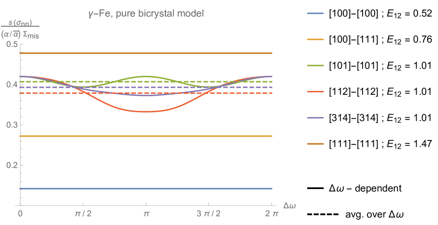
Figure 9: Standard deviation of $\sigma_{nn}$ distribution as a function of the twist-angle difference $\Delta\omega:=\omega_{2}-\omega_{1}$ for $\gamma$-Fe and six different GB types. For all of them maximal width of the corresponding INS distribution is reached at $\Delta\omega=0$. Dashed lines represent the twist-angle averaged values.

In Fig. 9 the influence of the twist angle is illustrated for several GB types. Specific choices have been made based on different criteria. Some GB types have been selected due to their independence from the twist angle $\Delta\omega$. This enables a direct comparison with the $\Delta\omega$-averaged outcomes presented in Fig. 8. Examples of such types include $[100]$-$[100]$, $[111]$-$[111]$, and $[100]$-$[111]$ configurations. They correspond to the softest and stiffest GBs in the aggregate, as well as the GBs sandwiched between the softest and stiffest grains along the GB-normal direction, respectively. The other three GB types, $[101]$-$[101]$, $[112]$-$[112]$, and $[314]$-$[314]$, are showcased because they all share a common value of $E_{12}$. Despite that, their $\Delta\omega$-averaged values of $s(\sigma_{nn})$ differ (albeit slightly, to the extent that this effect can be considered a next-order correction).

We can compute the value of $s(\sigma_{nn})$ as a function of $\Delta\omega$ for any GB type $[abc]$-$[def]$ in a given material. Analysis of the resulting expressions reveals that the INS distributions are the widest when the twist-angle difference between the two grains is set to zero. In Fig. 10, we show the maximal, minimal, and $\Delta\omega$-averaged values of $s(\sigma_{nn})$ for $\gamma$-Fe and the range of GB types obtained by selecting GB normals $(a,b,c)$ and $(d,e,f)$ from a set of $15$ preselected directions within the stereographic triangle.

The key observation is that the points associated with the maximal values of $[abc]$-$[abc]$-$\Delta\omega$ types (reached for $\Delta\omega=0$) are forming a smooth curve. This curve represents an upper bound for $s(\sigma_{nn})$ as a function of $E_{12}$. The $[abc]$-$[abc]$-$\Delta\omega$ GB types with $\Delta\omega=0$ correspond precisely to the single grain limit, which can be used for estimating the intragranular normal stresses, i.e., to calculate the stress perpendicular to a chosen plane within a single grain (modelled in this framework as a region of constant stress). In this limit, the relevant expressions simplify into:

$$s(\sigma_{nn}) =\frac{2\,|\alpha|}{(2\,s_{0}+s_{44})\,s_{44}}\,\sqrt{(6\,s_{11}\,s_{0}+6\,s_{11}\,s_{44}+s_{44}^{2})-\frac{6\,(s_{0}+s_{44})\,\hskip 1.00006pt\hbox{\vbox{\hrule height=0.5pt\kern 1.72218pt\hbox{\kern-1.00006pt$E$\kern-1.00006pt}}}\hskip 1.00006pt^{-1}}{E_{12}}}\times\frac{2}{3\sqrt{5}}\Sigma_{\text{mis}}\ .$$ (72)

The most important aspect of the solution presented above is that $s(\sigma_{nn})$ indeed becomes only a function of $E_{12}$. Hence, we succeeded in deriving the dependence of INS distribution’s width (in fact, its upper bound) on the effective stiffness, at least for specific GB types, if not in the general case, and thereby explicitly proved the significance of the $E_{12}$ parameter, justifying its prior use. However, the functional dependence in Eq. (72) is not of the form $s(\sigma_{nn})\approx A_{1}\arctan{\left(A_{2}\,E_{12}^{A_{3}}\right)}\,\Sigma_{\text{mis}}$, that successfully fits the $[abc]$-$[def]$ GB types averaged over $\Delta\omega$. Instead, it is described by a different relation, of the type $s(\sigma_{nn})=C_{1}\sqrt{1+C_{2}/E_{12}}\,\Sigma_{\text{mis}}$. Both sets of coefficients ($A_{k}$ and $C_{k}$) depend only on the material properties ($s_{11}$, $s_{12}$, and $s_{44}$).

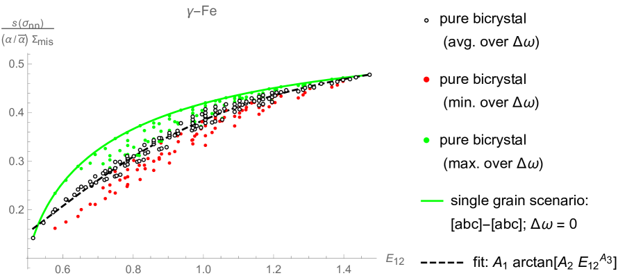
Figure 10: Maximal (green), minimal (red), and twist-angle averaged (black) values of the standard deviation $s(\sigma_{nn})$ for $120$ GB types corresponding to the selection of $(a,b,c)$ and $(d,e,f)$ from the $15$ preselected directions in the stereographic triangle, while keeping $\Delta\omega$ as a free parameter. The properties of $\gamma$-Fe have been chosen and inserted into the bicrystal solution, see Eqs. (63) and (56). The green curve represents the single grain solution specified in Eq. (72), while the dashed black line is the $A_{1}\arctan{\left(A_{2}\,E_{12}^{A_{3}}\right)}$ fit of $\Delta\omega$-averaged values. Normalization corresponds to uniaxial tensile loading ($\Sigma_{\text{mis}}=1$) and the average strain approximation ($\alpha=\hskip 0.90005pt\hbox{\vbox{\hrule height=0.5pt\kern 1.54996pt\hbox{\kern-0.90005pt$\alpha$\kern-0.90005pt}}}\hskip 0.90005pt=\frac{1}{2\,G}$).

For random twist angles, the expression (60) predicting the GB-normal stress in the bicrystal model simplifies to (for any lattice symmetry):

$$\sigma_{zz}^{\Delta\omega} =\hskip 1.00006pt\hbox{\vbox{\hrule height=0.5pt\kern 1.72218pt\hbox{\kern-1.00006pt$a$\kern-1.00006pt}}}\hskip 1.00006pt_{xx,yy}\,(\Sigma_{xx}+\Sigma_{yy})+\hskip 1.00006pt\hbox{\vbox{\hrule height=0.5pt\kern 1.72218pt\hbox{\kern-1.00006pt$a$\kern-1.00006pt}}}\hskip 1.00006pt_{zz}\,\Sigma_{zz}\ ,$$ (73)

where $\hskip 1.00006pt\hbox{\vbox{\hrule height=0.5pt\kern 1.72218pt\hbox{\kern-1.00006pt$a$\kern-1.00006pt}}}\hskip 1.00006pt_{ij}=(2\,\pi)^{-2}\int_{0}^{2\pi}\int_{0}^{2\pi}a_{ij}\,d\omega_{1}\,d\omega_{2}$, and $\hskip 1.00006pt\hbox{\vbox{\hrule height=0.5pt\kern 1.72218pt\hbox{\kern-1.00006pt$a$\kern-1.00006pt}}}\hskip 1.00006pt_{xx}=\hskip 1.00006pt\hbox{\vbox{\hrule height=0.5pt\kern 1.72218pt\hbox{\kern-1.00006pt$a$\kern-1.00006pt}}}\hskip 1.00006pt_{yy}:=\hskip 1.00006pt\hbox{\vbox{\hrule height=0.5pt\kern 1.72218pt\hbox{\kern-1.00006pt$a$\kern-1.00006pt}}}\hskip 1.00006pt_{xx,yy}$. This result also provides justification for the buffer-grain model [22], which arrived at the expression of a similar form. All the dependence on $\phi$ dropped out of it (while for uniaxial loading in the $Z$-direction, even the dependence on $\psi$ vanishes). Consequently,

$$\begin{split}s(\sigma_{nn}^{\Delta\omega})&=|\hskip 1.00006pt\hbox{\vbox{\hrule height=0.5pt\kern 1.72218pt\hbox{\kern-1.00006pt$a$\kern-1.00006pt}}}\hskip 1.00006pt_{xx,yy}-\hskip 1.00006pt\hbox{\vbox{\hrule height=0.5pt\kern 1.72218pt\hbox{\kern-1.00006pt$a$\kern-1.00006pt}}}\hskip 1.00006pt_{zz}|\times\frac{2}{3\sqrt{5}}\Sigma_{\text{mis}}\\ &=|\alpha|\,|\hskip 1.00006pt\hbox{\vbox{\hrule height=0.5pt\kern 1.72218pt\hbox{\kern-1.00006pt$c$\kern-1.00006pt}}}\hskip 1.00006pt_{xx,yy}-\hskip 1.00006pt\hbox{\vbox{\hrule height=0.5pt\kern 1.72218pt\hbox{\kern-1.00006pt$c$\kern-1.00006pt}}}\hskip 1.00006pt_{zz}|\times\frac{2}{3\sqrt{5}}\Sigma_{\text{mis}}\\ &=\frac{|\alpha|}{2}\,|(C_{11}+2\,C_{12})-3\,\hskip 1.00006pt\hbox{\vbox{\hrule height=0.5pt\kern 1.72218pt\hbox{\kern-1.00006pt$c$\kern-1.00006pt}}}\hskip 1.00006pt_{zz}|\times\frac{2}{3\sqrt{5}}\Sigma_{\text{mis}}\quad\text{(for cubic symmetry)}\ .\end{split}$$ (74)

4.4 Comparison with FE simulations

To compare the results of the bicrystal model with realistic stresses obtained in numerical simulations, we will examine the INS distributions generated by both approaches. We will focus on several representative GB types ($[100]$-$[100]$, $[102]$-$[334]$, and $[111]$-$[111]$) within a chosen material ($\gamma$-Fe).

Two scenarios will be considered: either the pure bicrystal model embedded in a homogeneous and isotropic neighbourhood, or introducing Gaussian fluctuations to induced stresses, meant to mimic the effect of anisotropic grains surrounding the bicrystal pair. In the latter case, an additional free parameter, $\sigma_{G}$, is required alongside $\alpha$ and $\beta$.

4.4.1 Pure bicrystal model

As demonstrated in Fig. 8, the bicrystal model, when combined with the average strain approximation (52), results in a standard deviation curve that is overly steep. To address this issue, we impose a less constraining condition on the bicrystal strain $\hskip 1.00006pt\hbox{\vbox{\hrule height=0.5pt\kern 1.72218pt\hbox{\kern-1.00006pt$\epsilon$\kern-1.00006pt}}}\hskip 1.00006pt^{b}_{ij}$, introducing two additional parameters, $\alpha$ and $\beta$, see Eq. (54). By appropriately adjusting their values, we can reconcile the discrepancies between the $s(\sigma_{nn})$ obtained from FE simulations and the model predictions. However, our goal extends beyond matching the standard deviation; we aim to fit the entire INS distribution, ensuring that all its moments agree with their predicted values.

For a chosen material ($C_{ij}$) and GB type ($a$, $b$, $c$, $d$, $e$, $f$), we can evaluate the first two moments of $\sigma_{nn}$ distribution in the bicrystal model, as described by Eqs. (62) and (63). Then $\alpha$ and $\beta$ can be determined by averaging those expressions over $\Delta\omega$ and fitting them to the FE values. Specifically, we need to solve the equations

$$\mu_{h}^{(1)} =\langle\sigma_{nn}\rangle_{h}=\mu_{f}^{(1)}\ ,$$ (75)

$$\mu_{h}^{(2)} =\langle(\sigma_{nn}-\langle\sigma_{nn}\rangle_{h})^{2}\rangle_{h}=\mu_{f}^{(2)}$$ (76)

for the first two moments of FE distribution $h$ and bicrystal distribution $f$, where

$$\mu_{f}^{(1)} =\langle\sigma_{nn}\rangle_{f}$$ (77)

$$=(\alpha-3\,\beta)\,(c_{xx}+c_{yy}+c_{zz})\times\frac{1}{3}\operatorname{Tr}\mathbf{\Sigma}\ ,$$

$$\mu_{f}^{(2)} =\langle(\sigma_{nn}-\langle\sigma_{nn}\rangle_{f})^{2}\rangle_{f}$$ (78)

$$=\alpha^{2}\left(\frac{1}{2}\,\big{(}(c_{xx}-c_{yy})^{2}+(c_{yy}-c_{zz})^{2}+(c_{zz}-c_{xx})^{2}\big{)}+3\,(c_{xy}^{2}+c_{xz}^{2}+c_{yz}^{2})\right)\times\frac{2}{15}\operatorname{Tr}(\mathbf{\Sigma}^{2}_{\text{dev}})\ .$$

In principle, both parameters, $\alpha$ and $\beta$, could vary with GB type and material properties, potentially assuming different values for each $E_{12}$ (at a given $A^{u}$). However, for cubic lattice symmetry, the relationship between $\alpha$ and $\beta$ is quite straightforward. In this limit, the requirement that the mean value should match $\tfrac{1}{3}\operatorname{Tr}\mathbf{\Sigma}$ for every GB type, effectively fixes the value of $\beta$, as indicated in Eq. (69). Consequently, we are left with just one adjustable parameter ($\alpha$). While it is possible to determine this parameter also through fitting to higher-order moments, the most precise approach typically involves using the standard deviation.

Upon inserting the values of $\alpha$ and $\beta$ into $\sigma_{nn}$, we can assess how accurately we have replicated the actual INS distributions. Fig. 11 features three distinct GB types: $[001]$-$[001]$, $[111]$-$[111]$, and $[102]$-$[334]$, representing the softest, stiffest, and an intermediate GB type. The choice of the latter has been motivated by the fact that its effective GB stiffness in $\gamma$-Fe is $E_{12}=0.97$, which closely matches the stiffness of isotropic grains ($E_{12}=1$) or the average stiffness of the aggregate (corresponding to random GBs, see Fig. 2).

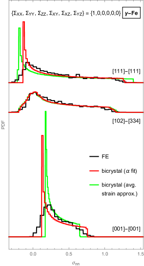
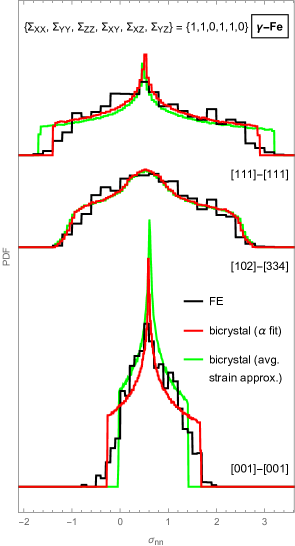
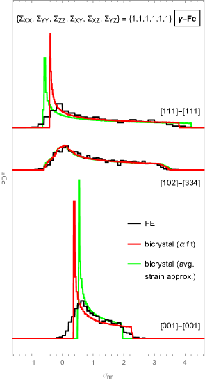
Figure 11: Comparison of (reduced) INS distributions from FE simulations (black; $N=1636$) with those from the (pure) bicrystal model. In the latter case, two variants are considered: using the average strain approximation $\alpha=1/(2\,G)$ (green) or determining the values of $\alpha$ and $\beta$ through fitting specified in Eqs. (75) and (76) (red). Results are presented for three external loadings and three different $\Delta\omega$-averaged GB types in $\gamma$-Fe. In each of these cases, the mean values of all three distributions are the same, while their standard deviations match only for the red and black curves.

It is worth noting that the same $\alpha$ was used for all loadings in Fig. 11, hence confirming the validity of the scaling factors $\operatorname{Tr}\mathbf{\Sigma}$ and $\Sigma_{\text{mis}}$ for the first two moments, respectively. Nonetheless, it is also evident that $\alpha$ and $\beta$ alone are insufficient to accurately reproduce the FE distributions.

4.4.2 Gaussian modulation

The approach taken in the previous section does not quite capture the genuine stress responses, particularly for very soft and very stiff GBs. For these GB types, the predicted INS distributions manifestly disagree with the outcomes of the FE simulations, see Fig. 11. It is evident that the predictions of the bicrystal model exhibit a notably sharper and narrower profile, despite the same “width” of distributions in both cases (specifically, the parameters $\alpha$ and $\beta$ have been adjusted to ensure the agreement between the mean value and standard deviation of both distributions).

The naive two-parameter fitting procedure thus needs to be extended to include the effect of the inhomogeneous neighbourhood of a bicrystal pair. In line with our perturbative framework (see also Eq. (13)), this extension can be conceptualized as follows:

$$\small\begin{split}\textbf{bicrystal model}+\textbf{Gaussian fluctuations}\approx&\,\textbf{INS distributions on individual GB types}\ .\end{split}\normalsize$$ (79)

The approach again involves convolution with normally distributed random fluctuations. Due to the additional parameter $\sigma_{G}$, we now have a three-parameter fitting procedure:

$$\mu_{h}^{(1)} =\langle\sigma_{nn}\rangle_{h}=\mu_{f}^{(1)}\ ,$$ (80)

$$\mu_{h}^{(2)} =\langle(\sigma_{nn}-\langle\sigma_{nn}\rangle_{h})^{2}\rangle_{h}=\mu_{f}^{(2)}+\sigma_{G}^{2}\ ,$$ (81)

$$\mu_{h}^{(3)} =\langle(\sigma_{nn}-\langle\sigma_{nn}\rangle_{h})^{3}\rangle_{h}=\mu_{f}^{(3)}\ ,$$ (82)

providing the values of $\alpha$, $\beta$, and $\sigma_{G}$. The first two statistical moments of the pure bicrystal distribution $f$ are provided in Eqs. (77) and (78), while the third is given by:

$$\mu_{f}^{(3)} =\langle(\sigma_{nn}-\langle\sigma_{nn}\rangle_{f})^{3}\rangle_{f}$$

$$\begin{split}&=\alpha^{3}\,\frac{1}{2}\,\Big{(}2\left(c_{xx}^{3}+c_{yy}^{3}+c_{zz}^{3}\right)+12\,c_{xx}\,c_{yy}\,c_{zz}+54\,c_{xy}\,c_{xz}\,c_{yz}+\\ &+9\left(c_{xx}\,(c_{xy}^{2}+c_{xz}^{2}-2\,c_{yz}^{2})+c_{yy}\,(c_{xy}^{2}+c_{yz}^{2}-2\,c_{xz}^{2})+c_{zz}\,(c_{xz}^{2}+c_{yz}^{2}-2\,c_{xy}^{2})\right)-\\ &-3\left(c_{xx}^{2}\,(c_{yy}+c_{zz})+c_{yy}^{2}\,(c_{xx}+c_{zz})+c_{zz}^{2}\,(c_{xx}+c_{yy})\right)\Big{)}\times\frac{8}{105}\operatorname{Tr}(\mathbf{\Sigma}^{3}_{\text{dev}})\ .\end{split}$$ (83)

The required moments of the convolution $h$ are obtained from the $\sigma_{nn}$ distribution produced in FE simulation. In principle, we could use any three moments $\mu_{h}^{(n)}$ for the fitting, but from practical perspective it is best to take the lowest-order moments because they are most accurate, especially when dealing with imprecisely known FE distributions (computed on only finite aggregate).

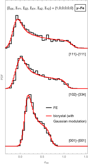
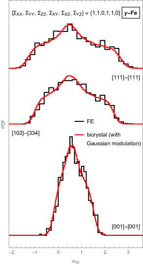
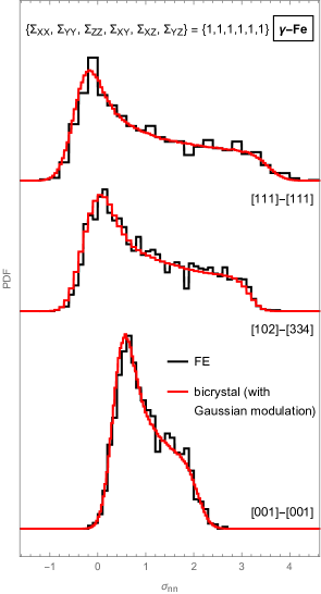
Figure 12: Same as in Fig. 11, but for the bicrystal model with Gaussian modulation. Parameters $\alpha$, $\beta$, and $\sigma_{G}/\Sigma_{\text{mis}}$ are determined from the lowest three statistical moments of FE distributions and depend only on the GB type, irrespective of the external loading. Thus, all three panels are generated using the same set of parameters.

With the fitted values of $\alpha$, $\beta$, and $\sigma_{G}$, we can now compare the convoluted bicrystal-model distributions with the FE results, as shown in Fig. 12. The agreement appears significantly improved compared to Fig. 11, which did not include the Gaussian fluctuations. However, the accuracy of the proposed method is constrained by the inherent imprecision of the FE results due to limited statistics. In particular, the FE simulations are based on only $1636$ GBs of a selected GB type, which is far from sufficient to produce a uniform distribution of GB orientations. In contrast, the bicrystal case employs $10^{6}$ random GBs, resulting in a much smoother distribution. For each specific GB type, the same values of $\alpha$, $\beta$, and $\sigma_{G}/\Sigma_{\text{mis}}$ have been used in all the panels of Fig. 12.

At last, in Fig. 13 we present a comparison between the bicrystal-model predictions and the full INS distributions, corresponding to normal stresses across all $159461$ finite elements associated with the GBs of a selected type. These distributions are wider than the reduced versions in Fig. 12, but given the substantial number of elements compared to the number of GBs, they also offer increased accuracy and detail.

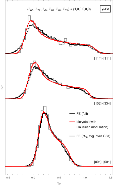
Figure 13: A comparison between the modelled (red) and realistic (black; $N=159461$) full INS distributions for $\gamma$-Fe, three different GB types (with random $\Delta\omega$), and uniaxial tensile loading. The values of $\alpha$, $\beta$, and $\sigma_{G}$ have been determined from the lowest three statistical moments of the (full) FE distributions. Additionally, the reduced INS distributions (gray; $N=1636$) are also displayed.

4.5 Fits across GB types and material properties

Up to this point, the procedure outlined in the previous section was completely general and applicable to any lattice symmetry. On the downside, it requires numerical simulations to determine for a given material and GB type the values of parameters $\alpha$, $\beta$, and $\sigma_{G}$, extracting them from the first three statistical moments of the FE distribution.

Given the absence of a mechanism to determine these parameters from first principles, our approach in this section is to fit them empirically. With the help of these approximate fits, one can almost instantaneously (and with minimal resources) estimate the INS distribution for any material and GB type, circumventing the need for extensive numerical simulations.

Here, we will focus only on materials with cubic lattices. In this particular scenario, the procedure simplifies in several significant aspects. First of all, just two parameters ($\alpha$ and $\sigma_{G}$) require fitting in this case, as $\beta$ is already fully determined by Eq. (69) due to the fact that, in cubic polycrystallines, $\langle\sigma_{nn}\rangle=\tfrac{1}{3}\,\operatorname{Tr}{\mathbf{\Sigma}}$ for any GB type. Secondly, for materials with cubic symmetry, $\alpha$ and $\sigma_{G}$ are solely functions of $E_{12}$, while for lower symmetries of the crystal lattice, they depend on additional parameters (such as $\nu_{12}$, see [22]). Thirdly, for non-cubic lattices, $\sigma_{G}$ does not precisely scale with $\Sigma_{\text{mis}}$, as evidenced by the material’s response to hydrostatic loading. And lastly, it also remains unclear to what extent we can approximate the fluctuation $\Delta\sigma_{nn}$ with a Gaussian distribution in that case.

Systematically exploring the parameter space of various cubic materials and GB types makes it possible to express (or rather fit) the parameters $\alpha$, $\beta$, and $\sigma_{G}/\Sigma_{\text{mis}}$ as functions of $A^{u}$ and $E_{12}$. For any material with cubic lattice symmetry, the parameter $\alpha$ roughly follows (neglecting the scatter in the bicrystal case) a decreasing exponential trend with respect to $E_{12}$:

$$\frac{\alpha}{\hskip 1.00006pt\hbox{\vbox{\hrule height=0.5pt\kern 1.72218pt\hbox{\kern-1.00006pt$\alpha$\kern-1.00006pt}}}\hskip 1.00006pt} =b_{1}\,E_{12}^{-b_{2}}\ .$$ (84)

Here, $\hskip 1.00006pt\hbox{\vbox{\hrule height=0.5pt\kern 1.72218pt\hbox{\kern-1.00006pt$\alpha$\kern-1.00006pt}}}\hskip 1.00006pt=(2\,G)^{-1}$ represents the value of $\alpha$ in the isotropic limit (cf. Footnote 17), while $b_{1}$ and $b_{2}$ denote some material-specific parameters. The width of Gaussian modulation ($\sigma_{G}$) required to match the full FE stress distribution is, to a good approximation, an increasing linear function of $E_{12}$:

$$\frac{\sigma_{G}}{\Sigma_{\text{mis}}} =d_{1}\,E_{12}+d_{2}\ .$$ (85)

For practical use, we provide here phenomenological fits of parameters $b_{1}$, $b_{2}$, $d_{1}$, and $d_{2}$ to the values of $A^{u}$, see Fig. 15. The following fitting functions have been selected for their simplicity and small number of fitting parameters (gathered in Table 1):

$$b_{1} =c_{1}\,\exp{\left(-c_{2}\,(A^{u})^{2}\right)}+(1-c_{1})\ ,$$ (86)

$$b_{2} =\left(c_{3}\,A^{u}+c_{4}\right)\,\hskip 1.00006pt\hbox{\vbox{\hrule height=0.5pt\kern 1.72218pt\hbox{\kern-1.00006pt$\nu$\kern-1.00006pt}}}\hskip 1.00006pt^{-1}\ ,$$ (87)

$$d_{1} =c_{5}\,(A^{u})^{1/4}\ ,$$ (88)

$$d_{2} =c_{6}\,(A^{u})^{1/2}\,\hskip 1.00006pt\hbox{\vbox{\hrule height=0.5pt\kern 1.72218pt\hbox{\kern-1.00006pt$\nu$\kern-1.00006pt}}}\hskip 1.00006pt\ .$$ (89)

Table 1: Optimal values of fitting parameters (for polycrystalline materials with cubic lattice symmetry), as were defined in Eqs. (86)–(89).

$c_{1}$	$c_{2}$	$c_{3}$	$c_{4}$		$c_{5}$	$c_{6}$
0.20	0.14	-0.0046	0.11		0.036	0.14

For demonstration purposes, a comparison between INS distributions produced by FE simulations and the bicrystal model using the above fits is shown in Figs. 16 and 17 for five different materials and several randomly selected GB types. A good agreement can be observed, despite a rather large uncertainty in the FE distribution obtained on an aggregate with only $4000$ grains. To assess its typical fluctuation, refer to Fig. 14, depicting the full INS distribution on a specific GB type using three different aggregates.

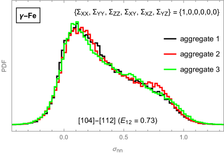
Figure 14: A full INS distribution for the $[104]$-$[112]$ GB type (with randomly assigned twist angles $\Delta\omega$) in $\gamma$-Fe under uniaxial loading. Comparison is shown between the FE simulation results obtained from three different Voronoi aggregates with $4000$ grains.

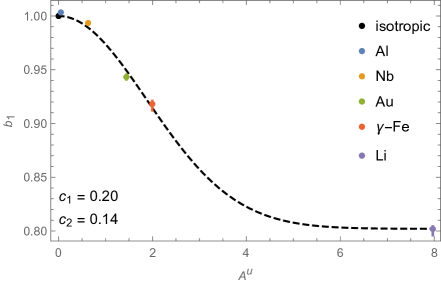
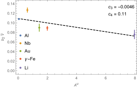
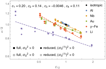
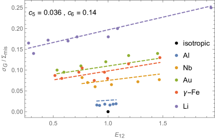
Figure 15: Bottom left: The parameter $\alpha$ was determined for various GB types and cubic materials by matching the third moments of the pure bicrystal model with either full (squares) or reduced (circles) FE distributions. Due to the imprecision of simulation results, the second moment of the pure bicrystal distribution can exceed that from FE (empty markers). Error bars indicate the estimated variation of FE distribution, either due to different loading configurations or different Voronoi aggregates. The dashed line represents the postulated $\alpha(E_{12})$ relation (84), based on fitting $b_{1}$ (top left) and $b_{2}$ (top right) to $A^{u}$ through expressions (86) and (87), respectively, where the error bars are due to slightly different values obtained from full and reduced distributions. Using Eq. (84) to assign the value to $\alpha$, the width of required Gaussian fluctuation $(\sigma_{G})$ is obtained by matching the second moment of the full FE distribution (bottom right). Dashed lines represent the fit (85) with $d_{1}$ and $d_{2}$ determined from Eqs. (88) and (89), respectively. The values from Table 1 have been used in all the dashed fits.

The $\alpha(E_{12},A^{u})$ and $\sigma_{G}(E_{12},A^{u})$ fits provided here should primarily be regarded only as a proof of concept, as the origin and exact form of functional dependency remain largely unknown at present. The main obstacle to their refinement represents the lack of accuracy in the obtained results, as fitted parameters are subject to substantial uncertainties due to limited statistical data. In practical terms, we would need either a larger aggregate or a substantial number of them for each GB type and material under consideration. Accumulating a sufficient number of data points in the $E_{12}$–$A^{u}$ plane should presumably lead to the identification of a more appropriate fitting functions.

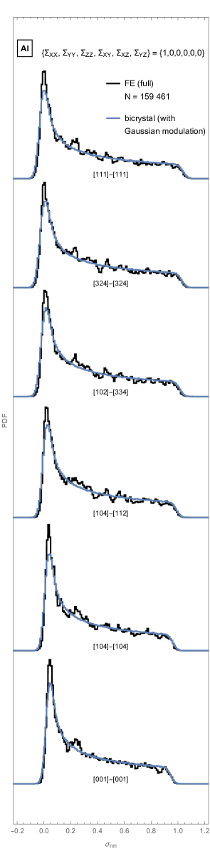
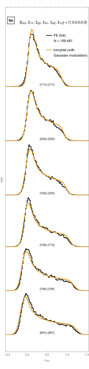
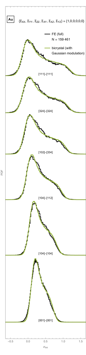
Figure 16: A comparison between the modelled (colored) and FE (black; $N=159461$) full INS distributions for several GB types (with random $\Delta\omega$) in Al, Nb, and Au under uniaxial tensile loading. The values of $\alpha$, $\beta$, and $\sigma_{G}$ have been determined from fits; cf. Eqs. (69), (84)–(89), and Table 1.

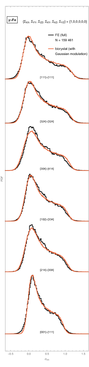
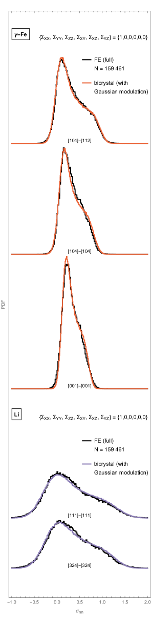
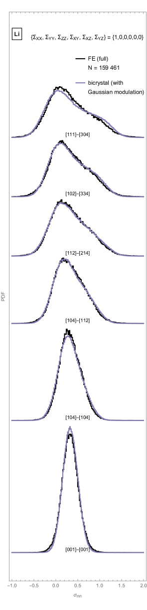
Figure 17: Same as in Fig. 16, but for $\gamma$-Fe and Li. The INS distribution for the $[104]$-$[112]$ GB type in $\gamma$-Fe is compiled from distributions on three different aggregates (with $4000$ grains each) and contains $478213$ finite elements. It is thus the smoothest and most accurate, see also Fig. 14 for a comparison between the three distributions in individual aggregates.

4.6 Alternative approach: the analysis of uniaxial loading

The drawback of the aforementioned procedure is its critical dependence on the accurate extraction of the first three statistical moments from numerical distributions obtained on a finite (and relatively small) aggregate.

As an alternative approach, we can use the bicrystal model to examine the INS distribution under uniaxial loading conditions. As will be demonstrated below, this distribution (for any chosen GB type) resembles the isotropic distribution. We can then extend it to apply to a selected uniform loading scenario. This extension can be achieved through the techniques outlined in [43], or by first generalizing the GB stresses according to Eq. (98) and then generating their distribution anew. Finally, the resulting pure bicrystal-model INS distribution should be convolved with a normal distribution (fluctuations).

In the bicrystal model, all GBs with the same orientation $\hat{n}$ correspond to equal $\sigma_{nn}$, whereas in a realistic aggregate, GB stresses can differ due to variations in the local neighbourhood of each GB. The distribution of these stresses exhibits a Gaussian profile. For uniaxial loading (of strength $\Sigma_{0}$), the average normal stress $\langle\sigma_{nn}\rangle_{\theta}$ on GBs with inclination $\theta$ relative to the loading direction is given by:

$$\frac{\langle\sigma_{nn}\rangle_{\theta}}{\Sigma_{0}} =k\,\cos^{2}\theta+n\ ,$$ (90)

where $k$ and $n$ are some material and GB-type dependent coefficients. This relation seems to hold universally, i.e., for any lattice symmetry, as illustrated in Fig. 18.

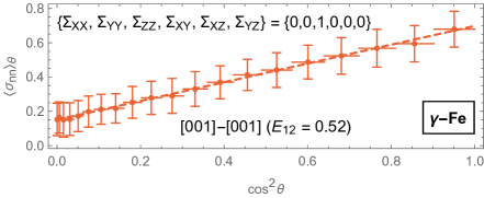
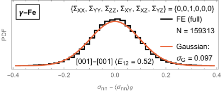
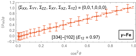
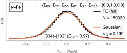
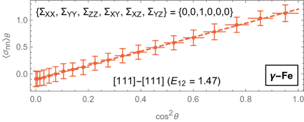
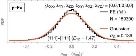
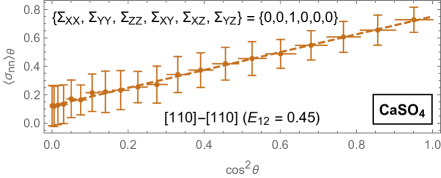
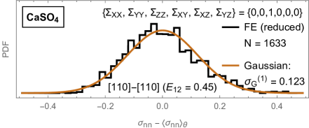
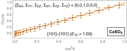
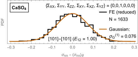
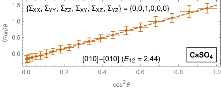
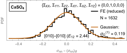
Figure 18: Left panels: The average value of $\sigma_{nn}$ across all GBs in the aggregate that are of a given type and have the same inclination $\theta$ with respect to uniaxial external loading. Horizontal lines indicate the width of the bin $\cos\theta\pm 0.025$, while vertical bars correspond to the standard deviation of the $\sigma_{nn}$ distribution in each bin. The dashed line is a linear fit (90) with $n$ defined in Eq. (91). Right panels: The distribution of normal stresses around their expected values (represented by the dashed line on the left) is again well-fitted by a Gaussian. Results are shown for three GB types and two selected materials.

The approximate value of the $y$-intercept ($n$) in Eq. (90) was determined in [22] to be:

$$n \approx-\frac{1}{3}\left(k-\frac{2\,(1+\nu_{12}-\hskip 1.00006pt\hbox{\vbox{\hrule height=0.5pt\kern 1.72218pt\hbox{\kern-1.00006pt$\nu$\kern-1.00006pt}}}\hskip 1.00006pt)}{E_{12}^{-1}+1}\right)\ ,$$ (91)

where the effective GB stiffness ($E_{12}$) is in general computed as:

$$E_{12}=2\,\hskip 1.00006pt\hbox{\vbox{\hrule height=0.5pt\kern 1.72218pt\hbox{\kern-1.00006pt$E$\kern-1.00006pt}}}\hskip 1.00006pt^{-1}\left(\tilde{s}_{3333}^{(1)}+\tilde{s}_{3333}^{(2)}\right)^{-1}\ ,$$ (92)

and the effective GB Poisson’s ratio ($\nu_{12}$) as:

$$\nu_{12} =-\frac{1}{4}\,\hskip 1.00006pt\hbox{\vbox{\hrule height=0.5pt\kern 1.72218pt\hbox{\kern-1.00006pt$E$\kern-1.00006pt}}}\hskip 1.00006pt\left(\tilde{s}_{1133}^{(1)}+\tilde{s}_{1133}^{(2)}+\tilde{s}_{2233}^{(1)}+\tilde{s}_{2233}^{(2)}\right)\ .$$ (93)

In crystals with cubic symmetry, the latter reduces to $\nu_{12}=\hskip 1.00006pt\hbox{\vbox{\hrule height=0.5pt\kern 1.72218pt\hbox{\kern-1.00006pt$\nu$\kern-1.00006pt}}}\hskip 1.00006pt+\tfrac{1}{2}(E_{12}^{-1}-1)$, thereby becoming a function of $E_{12}$. This results in $n^{\text{cubic}}=-\tfrac{1}{3}\,(k-1)$, yielding $\langle\sigma_{nn}\rangle=\Sigma_{0}/3$, as confirmed by numerical simulations.

For cubic lattices, the slope ($k$) is well-fitted by the following ansatz (see Fig. 19):

$$k^{\text{cubic}} =a_{1}\,E_{12}^{-a_{2}}+a_{3}\ ,$$ (94)

where $a_{1}$, $a_{2}$, and $a_{3}$ are material-dependent coefficients, presumably functions of only $A^{u}$ or $A$. A slightly different approximation was suggested in the context of the ($L_{n}=2$) buffer-grain model [22]:

$$k^{\text{cubic}} \approx\frac{3}{1+\left(E_{12}+f_{1}-\left|E_{12}-\frac{E_{12}^{\text{min}}+E_{12}^{\text{max}}}{2}\right|^{f_{2}}\right)^{-1}}-\frac{1}{2}\ ,$$ (95)

with

$$f_{1} =0.08\,(A^{u})^{0.85}\ ,$$ (96)

$$f_{2} =\frac{\log{f_{1}}}{\log{\frac{E_{12}^{\text{max}}-E_{12}^{\text{min}}}{2}}}\ ,$$ (97)

where $E_{12}^{\text{min}}=\hskip 1.00006pt\hbox{\vbox{\hrule height=0.5pt\kern 1.72218pt\hbox{\kern-1.00006pt$E$\kern-1.00006pt}}}\hskip 1.00006pt^{-1}/s_{11}$, and $E_{12}^{\text{max}}=\hskip 1.00006pt\hbox{\vbox{\hrule height=0.5pt\kern 1.72218pt\hbox{\kern-1.00006pt$E$\kern-1.00006pt}}}\hskip 1.00006pt^{-1}/(s_{11}-\tfrac{2}{3}\,s_{0})$ for $A\geq 1$ (and vice versa for $A<1$).

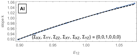
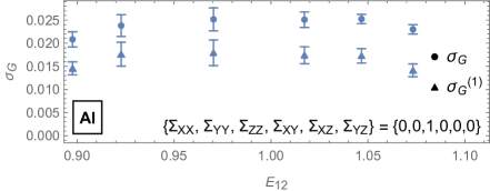
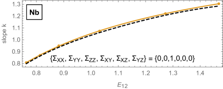
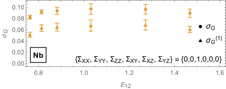
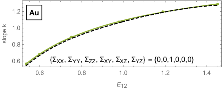
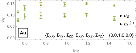
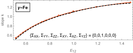
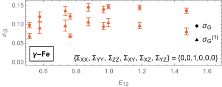
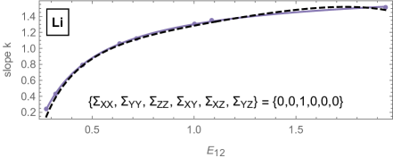
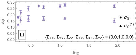
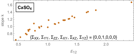
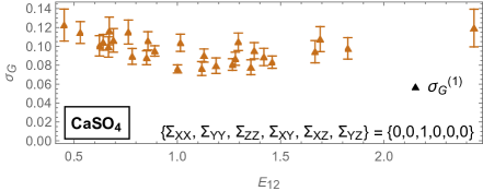
Figure 19: Left panels: The slope ($k$) as a function of effective GB stiffness ($E_{12}$) for various materials. For lattices with cubic symmetry, it is well-fitted by Eq. (94) (colored curves), while the fitting function (95) proposed in the context of the buffer-grain model [22] (black dashed curves) also provides a good fit. For non-cubic materials, the results are more scattered (indicating a dependence beyond just $E_{12}$). Right panels: The width of the Gaussian (and its uncertainty due to variation over different GB inclinations) obtained from fitting the full ($\sigma_{G}$) and reduced ($\sigma_{G}^{(1)}$) INS distributions.

For a general uniform loading, cubic lattice symmetry, and a random twist angle, the average GB-normal stress across all GBs with the same inclination $\hat{n}$ is:

$$\langle\sigma_{nn}\rangle_{\hat{n}} =\tfrac{1}{3}\,(2\,k+1)\,\Sigma_{zz}-\tfrac{1}{3}\,(k-1)\,(\Sigma_{xx}+\Sigma_{yy})\ ,$$ (98)

(with the components $\Sigma_{ij}$ given in Appendix B), while in the bicrystal model (under identical conditions), it is given by Eq. (73). Under uniaxial loading along the $Z$-direction, the latter further reduces to the linear trend (90) observed in FE simulations:

$$\frac{\sigma_{zz}^{\Delta\omega}}{\Sigma_{0}} =\alpha\,(\hskip 1.00006pt\hbox{\vbox{\hrule height=0.5pt\kern 1.72218pt\hbox{\kern-1.00006pt$c$\kern-1.00006pt}}}\hskip 1.00006pt_{zz}-\hskip 1.00006pt\hbox{\vbox{\hrule height=0.5pt\kern 1.72218pt\hbox{\kern-1.00006pt$c$\kern-1.00006pt}}}\hskip 1.00006pt_{xx,yy})\cos^{2}\theta+\left(\alpha\,\hskip 1.00006pt\hbox{\vbox{\hrule height=0.5pt\kern 1.72218pt\hbox{\kern-1.00006pt$c$\kern-1.00006pt}}}\hskip 1.00006pt_{xx,yy}-\beta\,(2\,\hskip 1.00006pt\hbox{\vbox{\hrule height=0.5pt\kern 1.72218pt\hbox{\kern-1.00006pt$c$\kern-1.00006pt}}}\hskip 1.00006pt_{xx,yy}+\hskip 1.00006pt\hbox{\vbox{\hrule height=0.5pt\kern 1.72218pt\hbox{\kern-1.00006pt$c$\kern-1.00006pt}}}\hskip 1.00006pt_{zz})\right)\ .$$ (99)

By taking into account Eqs. (67) and (69), it can be shown that for cubic crystal lattices, $n$ is indeed equal to $n^{\text{cubic}}=-\tfrac{1}{3}(k-1)$:

$$\frac{\sigma_{zz}^{\Delta\omega}}{\Sigma_{0}} =\tfrac{1}{2}\,\alpha\left(3\,\hskip 1.00006pt\hbox{\vbox{\hrule height=0.5pt\kern 1.72218pt\hbox{\kern-1.00006pt$c$\kern-1.00006pt}}}\hskip 1.00006pt_{zz}-(C_{11}+2\,C_{12})\right)\cos^{2}\theta-\tfrac{1}{3}\left(\tfrac{1}{2}\,\alpha(3\,\hskip 1.00006pt\hbox{\vbox{\hrule height=0.5pt\kern 1.72218pt\hbox{\kern-1.00006pt$c$\kern-1.00006pt}}}\hskip 1.00006pt_{zz}-(C_{11}+2\,C_{12}))-1\right)\ .$$ (100)

From either of these two expressions, the slope $k$ and the $y$-intercept $n$ can be readily extracted. Comparing these values to those obtained from FE simulations allows us to determine the values of $\alpha$ and $\beta$. As shown in Fig. 20, for cubic lattices they can be effectively fitted by Eqs. (84) and (69), where the coefficients $b_{1}$ and $b_{2}$ in Fig. 21 exhibit similar trends as those observed in the previous section, following the relationships in Eqs. (86) and (87). The fitting coefficients ($c_{1}=0.22$, $c_{2}=0.15$, $c_{3}=-0.0074$, and $c_{4}=0.12$) possess only marginally different values from those listed in Table 1.

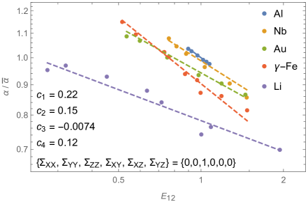
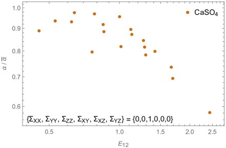
Figure 20: The parameter $\alpha$ plotted against effective GB stiffness $E_{12}$ for various materials. For lattices with cubic symmetry (left panel), the dependence is well-fitted by Eq. (84) (dashed curves), with $b_{1}$ and $b_{2}$ related to material’s anisotropy $A^{u}$ through Eqs. (86) and (87), respectively, and the values of fitting parameters listed in the inset. For non-cubic materials (right panel), the results are more scattered (suggesting a dependence beyond $E_{12}$). The value of $\alpha$ is normalized to its average strain approximation, $\hskip 0.90005pt\hbox{\vbox{\hrule height=0.5pt\kern 1.54996pt\hbox{\kern-0.90005pt$\alpha$\kern-0.90005pt}}}\hskip 0.90005pt:=(1+\hskip 0.90005pt\hbox{\vbox{\hrule height=0.5pt\kern 1.54996pt\hbox{\kern-0.90005pt$\nu$\kern-0.90005pt}}}\hskip 0.90005pt)/\hskip 0.90005pt\hbox{\vbox{\hrule height=0.5pt\kern 1.54996pt\hbox{\kern-0.90005pt$E$\kern-0.90005pt}}}\hskip 0.90005pt$ (which for cubic symmetry simplifies to $\hskip 0.90005pt\hbox{\vbox{\hrule height=0.5pt\kern 1.54996pt\hbox{\kern-0.90005pt$\alpha$\kern-0.90005pt}}}\hskip 0.90005pt\to\frac{1}{2G}$), see Eq. (52).

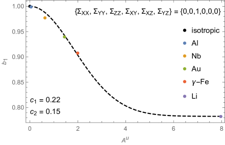
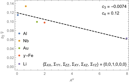
Figure 21: The parameters $b_{1}$ (left panel) and $b_{2}$ (right panel) plotted against the universal anisotropy index $A^{u}$. The dependencies are effectively captured by Eqs. (86) and (87), respectively (shown as dashed curves).

5 Discussion

The perturbative model presented in this paper displays several limitations and weaknesses. It is inherently probabilistic, primarily suited for estimating INS distributions rather than determining the stresses on specific GBs. Consequently, the model can help us assess only the statistical likelihood for microcrack initiation, but it does not allow us to pinpoint their exact locations.

Furthermore, the model’s validity is confined to the elastic regime since it does not account for plastic deformations, despite their crucial role in the formation of stress concentrations responsible for initiating the cracks. Another drawback of the model is the assumption of constant stress and strain throughout the grains and along their GBs. When making a direct comparison with realistic distributions, this corresponds to averaging the GB stresses over the respective GB areas. And while we typically assume that the stresses on each GB follow a normal distribution, this remains unconfirmed at this point. Lastly, it should also be mentioned that although our analytical solution was developed for a general case, many of the derived expressions and results provided here are valid only for cubic crystal lattices and grains of equal size ($V_{1}=V_{2}$).

In principle, the entire “machinery” of the bicrystal model, particularly Eqs. (56)–(59), was developed only to determine the parameters $\alpha$, $\beta$, and $\sigma_{G}$. However, once their fits are obtained, we can either numerically solve the constitutive equations for a chosen GB orientation and GB type, or use their analytical solution (60) for the coefficients defined in Eqs. (61) and (56). After producing the distribution across different GB orientations (and twist angles), we must convolve it with a Gaussian to obtain the actual (realistic) INS distribution.

Below are the detailed steps for producing the INS distribution for a chosen GB type in a selected material with cubic lattice symmetry under a given uniform external loading:

1. For a chosen material ($A^{u}$), GB type ($E_{12}$), and uniform external loading ($\mathbf{\Sigma}$), compute the values of $\alpha$, and $\beta$ from fits in Eqs. (84), (86), (87), and (69). This allows us to produce $\sigma_{nn}$ (in the pure bicrystal model) by numerically solving Eqs. (38) and (49)–(51) along with condition (54) for any given GB orientation ($\psi$, $\cos\theta$, $\phi$) and twist angles ($\omega_{1}$ and $\omega_{2}$).

2. By taking a uniform distribution of these angles, we can produce the INS distribution in the pure bicrystal model (e.g., by Monte Carlo sampling).

3. Convolve the resulting distribution with the Gaussian distribution of width $\sigma_{G}$, obtained from fits in Eqs. (85) , (88), and (89).

While the presented bicrystal model is, in a sense, “exact”, the proposed phenomenological fits of $\alpha$ and $\sigma_{G}$ as functions of $E_{12}$, and especially of $A^{u}$, are not. They are only approximate and are meant only as a proof of concept. Beside the fact that there is no motivation for the chosen fitting functions beyond their simplicity and small number of parameters, also the fitted values are subject to significant uncertainties due to the smallness of the used aggregate, containing just $1636$ GBs of a chosen GB type. This effect becomes apparent when considering INS distributions under equivalent (i.e., rotated) loadings (such as $\{\Sigma_{XX},\Sigma_{YY},\Sigma_{ZZ},\Sigma_{XY},\Sigma_{XZ},\Sigma_{YZ}\}=\{1,0,0,0,0,0\}$ and $\{1,1,1,1,1,1\}$ in Fig. 12), which should generate identical distributions for an infinitely large aggregate, whereas for the aggregate used in practice, the moments can vary by as much as a few percent. The variation is significant enough that it can even mean the difference between the existence and non-existence of a solution (80)–(82) with real-valued $\alpha$, $\beta$, and $\sigma_{G}$. Those are, in fact, needed to be able to produce the fits in the first place.

Although the proposed fits perform reasonably well with a handful of fitting parameters, more accurate fits (both in terms of more suitable fitting functions and refined values of fitting coefficients) could likely be found. For instance, using a non-trivial distribution of grain sizes in the bicrystal model ($V_{1}\neq V_{2}$) or considering additional variables besides $E_{12}$ and $A^{u}$ could enhance the accuracy of the fits. This would require more extensive numerical data, including larger aggregates, a broader range of materials, GB types, and loadings.

Other potential sources of discrepancies with realistic distributions include: the use of the bicrystal-strain condition (54) with GB-orientation-independent parameters $\alpha$ and $\beta$ in the pure bicrystal model. However, the actual relevance of this assumption is best demonstrated by the fact that the same values of $\alpha$ and $\beta$ apply to both the reduced (i.e., averaged over the GB) and the full INS distribution, with only the width of Gaussian modulation (the value of $\sigma_{G}$) changing.

Another possible issue arises from the assumption that $\alpha$, $\beta$, and $\sigma_{G}$ are (only) functions of $E_{12}$ and $A^{u}$, and that the fluctuation ($\Delta\sigma_{nn}$) is Gaussian. And while $\alpha$ and $\beta$ are loading-independent, it is still not entirely clear how $\sigma_{G}$ correctly scales with loading. It is assumed that for cubic crystal lattices it is proportional to $\Sigma_{\text{mis}}$, but for non-cubic lattices, it remains an open question.

6 Conclusions

In the first part of the paper, we have demonstrated that we can successfully predict the INS distribution on random GBs for any polycrystalline material under uniform loading conditions. A single parameter was needed that connected the width of Gaussian fluctuations with the material’s anisotropy. This parameter was determined from numerical fits.

In the second part of the paper, we have shown how to generate INS distributions on particular GB types. This can again be done for any material and loading configuration, but for simplicity reasons, we restricted our analysis to lattices with cubic symmetry. In this case, instead of three parameters ($\alpha$, $\beta$, and $\sigma_{G}$), only two suffice to determine the INS distribution for a chosen GB type within a given material since $\alpha$ and $\beta$ are not independent of each other (in large part because the average Young’s modulus and the average Poisson’s ratio of the material are not linearly independent quantities in cubic crystals).

A simple functional dependence between $\alpha$ and $E_{12}$ has been proposed, with material-specific coefficients determined for several different materials, and correlated with their $A^{u}$. Similarly for $\sigma_{G}$. The existing fits involve just six parameters, the numerical values of which need to be determined only once. Improvement of these fits could make the bicrystal model extremely useful for quick and reliable predictions of INS distributions for any chosen GB type, material, and uniform external loading conditions. As such, it can serve as a valuable tool for estimating the probability of intergranular cracking initiation or for determining the GB strengths of selected GB types. A statistical knowledge of stresses (INS), resulting from a microscopic description (bicrystal model), can thus be used to address a macroscopic phenomenon (intergranular cracking initiation).

Appendix A Elastic properties of materials

In Table 2 elastic constants of single crystals (monocrystals), together with their aggregate properties, are listed for several representative materials used in this study. Chosen polycrystallines have either orthorhombic or cubic lattice symmetry. The materials are ordered according to their universal elastic anisotropy index $A^{u}$ [38] defined as

$$A^{u} =5\frac{G^{V}}{G^{R}}+\frac{K^{V}}{K^{R}}-6\ ,$$ (101)

where $G$ and $K$ are their shear and compression elastic moduli in Voigt ($V$) and Reuss ($R$) limits, respectively, which for macroscopically isotropic (untextured) polycrystallines assume the following forms [46]

$$K^{V} =\tfrac{1}{9}\big{(}C_{11}+C_{22}+C_{33}+2\,(C_{12}+C_{13}+C_{23})\big{)}\ ,$$ (102)

$$G^{V} =\tfrac{1}{15}\big{(}C_{11}+C_{22}+C_{33}+3\,(C_{44}+C_{55}+C_{66})-(C_{12}+C_{13}+C_{23})\big{)}\ ,$$ (103)

$$K^{R} =\big{(}s_{11}+s_{22}+s_{33}+2\,(s_{12}+s_{13}+s_{23})\big{)}^{-1}\ ,$$ (104)

$$G^{R} =\left(\tfrac{1}{15}\big{(}4\,(s_{11}+s_{22}+s_{33})+3\,(s_{44}+s_{55}+s_{66})-4\,(s_{12}+s_{13}+s_{23})\big{)}\right)^{-1}\ .$$ (105)

For cubic lattice symmetry, $C_{11}=C_{22}=C_{33}$, $C_{12}=C_{13}=C_{23}$ and $C_{44}=C_{55}=C_{66}$, hence the universal anisotropy index reduces to

$$A^{u} =\frac{3\,(C_{11}-C_{12}-2\,C_{44})^{2}}{5\,(C_{11}-C_{12})\,C_{44}}=\frac{6\,(A-1)^{2}}{5A}\ ,$$ (106)

where

$$A=\frac{2\,C_{44}}{C_{11}-C_{12}}$$ (107)

represents the Zener elastic anisotropy index [40] of the material. It is defined only for cubic lattices, with $A=1$ (and $A^{u}=0$) denoting a perfectly isotropic crystal.

Table 2: Elasticity (stiffness) tensor components $C_{ij}$ (in Voigt notation) of single crystals with orthorhombic ($\dagger$) [47] or cubic ($\ast$) [48] lattice symmetry, and their aggregate properties in polycrystallines (with    $E$   and    $\nu$   denoting the average Young’s modulus and Poisson’s ratio of a macroscopic aggregate, which are for cubic materials computed according to Eqs. (33) and (53), respectively). $C_{ij}$ and    $E$   are given in GPa.

Crystal	$C_{11}$	$C_{22}$	$C_{33}$	$C_{12}$	$C_{13}$	$C_{23}$	$C_{44}$	$C_{55}$	$C_{66}$	$E$	$\nu$	$A^{u}$	$A$
∗Al	107.3			60.9			28.3			70.41	0.346	0.05	1.22
∗Nb	240.2			125.6			28.2			104.9	0.393	0.63	0.49
∗Au	192.9			163.8			41.5			79.40	0.424	1.44	2.85
${}^{\ast}\gamma$-Fe	197.5			125.0			122.0			195.2	0.282	2.00	3.37
†CaSO4	93.82	185.5	111.8	16.51	15.20	31.73	32.47	26.53	9.26	71.77	0.282	2.78	/
∗Li	13.5			11.44			8.78			10.94	0.350	7.97	8.52

Appendix B Most general uniform external loading tensor $\mathbf{\Sigma}^{\text{lab}}$ expressed in GB coordinate system

$$\begin{split}\Sigma_{xx}&=\left(\sin^{2}\theta\,\cos^{2}\phi\right)\,\Sigma_{ZZ}+\left(\cos\theta\,\cos\psi\,\cos\phi-\sin\psi\,\sin\phi\right)^{2}\,\Sigma_{XX}+\\ &+\left(\cos\theta\,\sin\psi\,\cos\phi+\cos\psi\,\sin\phi\right)^{2}\,\Sigma_{YY}+\\ &+\left(\cos^{2}\theta\,\sin 2\psi\,\cos^{2}\phi+\cos\theta\,\cos 2\psi\,\sin 2\phi-\sin 2\psi\,\sin^{2}\phi\right)\,\Sigma_{XY}+\\ &+\sin\theta\left(\sin\psi\,\sin 2\phi-2\,\cos\theta\,\cos\psi\,\cos^{2}\phi\right)\,\Sigma_{XZ}-\\ &-2\sin\theta\,\cos\phi\left(\cos\theta\,\sin\psi\,\cos\phi+\cos\psi\,\sin\phi\right)\,\Sigma_{YZ}\ ,\end{split}$$ (108)

$$\begin{split}\Sigma_{yy}&=\left(\sin^{2}\theta\,\sin^{2}\phi\right)\,\Sigma_{ZZ}+\left(\cos\theta\,\cos\psi\,\sin\phi+\sin\psi\,\cos\phi\right)^{2}\,\Sigma_{XX}+\\ &+\left(\cos\psi\,\cos\phi-\cos\theta\,\sin\psi\,\sin\phi\right)^{2}\,\Sigma_{YY}+\\ &+\left(\cos^{2}\theta\,\sin 2\psi\,\sin^{2}\phi-\cos\theta\,\cos 2\psi\,\sin 2\phi-\sin 2\psi\,\cos^{2}\phi\right)\,\Sigma_{XY}-\\ &-2\sin\theta\,\sin\phi\left(\cos\theta\,\cos\psi\,\sin\phi+\sin\psi\,\cos\phi\right)\,\Sigma_{XZ}+\\ &+\sin\theta\left(\cos\psi\,\sin 2\phi-2\,\cos\theta\,\sin\psi\,\sin^{2}\phi\right)\,\Sigma_{YZ}\ ,\end{split}$$ (109)

$$\begin{split}\Sigma_{zz}&=\left(\cos^{2}\theta\right)\,\Sigma_{ZZ}+\left(\sin^{2}\theta\,\cos^{2}\psi\right)\,\Sigma_{XX}+\left(\sin^{2}\theta\,\sin^{2}\psi\right)\,\Sigma_{YY}+\\ &+\left(\sin^{2}\theta\,\sin 2\psi\right)\,\Sigma_{XY}+\left(\sin 2\theta\,\cos\psi\right)\,\Sigma_{XZ}+\left(\sin 2\theta\,\sin\psi\right)\,\Sigma_{YZ}\ ,\end{split}$$ (110)

$$\begin{split}\Sigma_{xy}&=-\left(\sin^{2}\theta\,\sin\phi\,\cos\phi\right)\,\Sigma_{ZZ}-\\ &-\frac{1}{2}\left(\cos^{2}\theta\,\cos^{2}\psi\,\sin 2\phi+\cos\theta\,\sin 2\psi\,\cos 2\phi-\sin^{2}\psi\,\sin 2\phi\right)\,\Sigma_{XX}-\\ &-\frac{1}{2}\left(\cos^{2}\theta\,\sin^{2}\psi\,\sin 2\phi-\cos\theta\,\sin 2\psi\,\cos 2\phi-\cos^{2}\psi\,\sin 2\phi\right)\,\Sigma_{YY}-\\ &-\frac{1}{2}\left(\left(\cos^{2}\theta+1\right)\sin 2\psi\,\sin 2\phi-2\,\cos\theta\,\cos 2\psi\,\cos 2\phi\right)\,\Sigma_{XY}+\\ &+\sin\theta\left(\cos\theta\,\cos\psi\,\sin 2\phi+\sin\psi\,\cos 2\phi\right)\,\Sigma_{XZ}+\\ &+\sin\theta\left(\cos\theta\,\sin\psi\,\sin 2\phi-\cos\psi\,\cos 2\phi\right)\,\Sigma_{YZ}\ ,\end{split}$$ (111)

$$\begin{split}\Sigma_{xz}&=-\left(\sin\theta\,\cos\theta\,\cos\phi\right)\,\Sigma_{ZZ}+\sin\theta\,\cos\psi\left(\cos\theta\,\cos\psi\,\cos\phi-\sin\psi\,\sin\phi\right)\,\Sigma_{XX}+\\ &+\sin\theta\,\sin\psi\left(\cos\theta\,\sin\psi\,\cos\phi+\cos\psi\,\sin\phi\right)\,\Sigma_{YY}+\\ &+\sin\theta\left(\cos\theta\,\sin 2\psi\,\cos\phi+\cos 2\psi\,\sin\phi\right)\,\Sigma_{XY}+\\ &+\left(\cos 2\theta\,\cos\psi\,\cos\phi-\cos\theta\,\sin\psi\,\sin\phi\right)\,\Sigma_{XZ}+\\ &+\left(\cos\theta\,\cos\psi\,\sin\phi+\cos 2\theta\,\sin\psi\,\cos\phi\right)\,\Sigma_{YZ}\ ,\end{split}$$ (112)

$$\begin{split}\Sigma_{yz}&=\left(\sin\theta\,\cos\theta\,\sin\phi\right)\,\Sigma_{ZZ}-\sin\theta\,\cos\psi\left(\cos\theta\,\cos\psi\,\sin\phi+\sin\psi\,\cos\phi\right)\,\Sigma_{XX}-\\ &-\sin\theta\,\sin\psi\left(\cos\theta\,\sin\psi\,\sin\phi-\cos\psi\,\cos\phi\right)\,\Sigma_{YY}-\\ &-\sin\theta\left(\cos\theta\,\sin 2\psi\,\sin\phi-\cos 2\psi\,\cos\phi\right)\,\Sigma_{XY}-\\ &-\left(\cos 2\theta\,\cos\psi\,\sin\phi+\cos\theta\,\sin\psi\,\cos\phi\right)\,\Sigma_{XZ}+\\ &+\left(\cos\theta\,\cos\psi\,\cos\phi-\cos 2\theta\,\sin\psi\,\sin\phi\right)\,\Sigma_{YZ}\end{split}$$ (113)

References

- [1] H. Nishioka, K. Fukuya, K. Fujii, and T. Torimaru, “IASCC initiation in highly irradiated stainless steels under uniaxial constant load conditions,” J. Nuc. Sci. and Tech., vol. 45, pp. 1072–1077, 2008.
- [2] M. Le Millier, O. Calonne, J. Crépin, C. Duhamel, L. Fournier, F. Gaslain, E. Héripré, O. Toader, Y. Vidalenc, and G. Was, “Influence of strain localization on IASCC of proton irradiated 304L stainless steel in simulated PWR primary water,” in 16th International Conference on Environmental Degragation of Materials in Nuclear Power Systems - Water Reactors, 2013.
- [3] K. Stephenson and G. Was, “Crack initiation behavior of neutron irradiated model and commercial stainless steels in high temperature water,” J. Nuc. Mat., vol. 444, pp. 331–341, 2014.
- [4] J. Gupta, J. Hure, B. Tanguy, L. Laffont, M. Lafont, and E. Andrieu, “Evaluation of stress corrosion cracking of irradiated 304 stainless steel in PWR environment using heavy ion irradiation,” J. Nuc. Mat., vol. 476, pp. 82–92, 2016.
- [5] T. Fujii, K. Tohgo, Y. Mori, Y. Miura, and Y. Shimamura, “Crystallographic and mechanical investigation of intergranular stress corrosion crack initiation in austenitic stainless steel,” Mat. Sci. Eng. A, vol. 751, pp. 160–170, 2019.
- [6] B. Cox, “Environmentally induced cracking of zirconium alloys,” tech. rep., Atomic Energy of Canada Limited, 1970.
- [7] B. Cox, “Envrionmentally-induced cracking of zirconium alloys - A review,” J. Nuc. Mat, vol. 170, pp. 1–23, 1990.
- [8] D. Van Rooyen, “Review of the stress corrosion cracking of inconel 600,” Corrosion, vol. 31, pp. 327–337, 1975.
- [9] C. Shen and P. Shewmon, “A mechanism for hydrogen-induced intergranular stress corrosion cracking in alloy 600,” Metall. Trans. A., vol. 21A, pp. 1261–1271, 1990.
- [10] J. Panter, B. Viguier, J. Cloué, M. Foucault, P. Combrade, and E. Andrieu, “Influence of oxide films on primary water stress corrosion cracking initiation of alloy 600,” J. Nuc. Mat., vol. 348, pp. 213–221, 2006.
- [11] IAEA, “Stress corrosion cracking in light water reactors: Good practices and lessons learned,” NP-T-3.13, IAEA Nuclear Energy Series, 2011.
- [12] M. Speidel, “Stress corrosion cracking of aluminum alloys,” Metallurgical and Materials Transactions A, vol. 6A, pp. 631–651, 1975.
- [13] T. Burleigh, “The postulated mechanisms for stress corrosion cracking of aluminum alloys: A review of the literature 1980-1989,” Corrosion, vol. 47, pp. 89–98, 1991.
- [14] Z. Wang and A. Atrens, “Initiation of stress corrosion cracking for pipeline steels in a carbonate-bicarbonate solution,” Metallurgical and Materials Transactions A, vol. 27A, pp. 2686–2691, 1996.
- [15] M. Arafin and J. Szpunar, “A new understanding of intergranular stress corrosion cracking resistance of pipeline steel through grain boundary character and crystallographic texture studies,” Corrosion Science, vol. 51, pp. 119–128, 2009.
- [16] E. A. West and G. S. Was, “A model for the normal stress dependence of intergranular cracking of irradiated 316L stainless steel in supercritical water,” Journal of Nuclear Materials, vol. 408, no. 2, pp. 142 – 152, 2011.
- [17] A. Stratulat, J. A. Duff, and T. J. Marrow, “Grain boundary structure and intergranular stress corrosion crack initiation in high temperature water of a thermally sensitised austenitic stainless steel, observed in situ,” Corrosion Science, vol. 85, pp. 428 – 435, 2014.
- [18] Z. Zhang, S. Xia, Q. Bai, T. Liu, H. Li, B. Zhou, L. Wang, and W. Ma, “Effects of 3D grain boundary geometrical angles and the net normal stress on intergranular stress corrosion cracking initiation in a 316 stainless steel,” Materials Science and Engineering: A, vol. 765, p. 138277, 2019.
- [19] G. Sfantos and M. Aliabadi, “Multi-scale boundary element modelling of material degradation and fracture,” Computer Methods in Applied Mechanics and Engineering, vol. 196, pp. 1310–1329, 01 2007.
- [20] I. Benedetti and M. Aliabadi, “A three-dimensional grain boundary formulation for microstructural modeling of polycrystalline materials,” Computational Materials Science, vol. 67, pp. 249–260, 2013.
- [21] I. Benedetti and M. Aliabadi, “A three-dimensional cohesive-frictional grain-boundary micromechanical model for intergranular degradation and failure in polycrystalline materials,” Computer Methods in Applied Mechanics and Engineering, vol. 265, pp. 36–62, 2013.
- [22] S. El Shawish and T. Mede, “Grain boundary stresses in elastic materials,” European Journal of Mechanics - A/Solids, vol. 99, p. 104940, 2023.
- [23] O. Diard, S. Leclercq, G. Rousselier, and G. Cailletaud, “Evaluation of finite element based analysis of 3D multicrystalline aggregates plasticity. Application to crystal plasticity model identification and the study of strain fields near grain boundaries,” Int. J. Plasticity, vol. 21, pp. 691–722, 2005.
- [24] O. Diard, S. Leclercq, G. Rousselier, and G. Cailletaud, “Distribution of normal stress at grain boundaries in multicrystals: Application to an intergranular damage modeling,” Comp. Mat. Sci., vol. 25, pp. 73–84, 2002.
- [25] A. Kanjarla, P. Van Houtte, and L. Delannay, “Assessment of plastic heterogeneity in grain interaction models using crystal plasticity finite element method,” Int. J. Plasticity, vol. 26, pp. 1220–1233, 2010.
- [26] D. Gonzalez, I. Simonovski, P. Withers, and J. Quinta da Fonseca, “Modelling the effect of elastic and plastic anisotropies on stresses at grain boundaries,” Int. J. Plasticity, vol. 61, pp. 49–63, 2014.
- [27] J. Hure, S. El Shawish, L. Cizelj, and B. Tanguy, “Intergranular stress distributions in polycrystalline aggregates of irradiated stainless steel,” J. Nuc. Mat., 2016.
- [28] S. El Shawish and J. Hure, “Intergranular normal stress distributions in untextured polycrystalline aggregates,” Eur. J. Mech. / A Solids, vol. 72, pp. 354–373, 2018.
- [29] R. Lebensohn, A. Kanjarla, and P. Eisenlohr, “An elasto-viscoplastic formulation based on fast fourier transforms for the prediction of micromechanical fields in polycrystalline materials,” Int. J. Plasticity, vol. 32-33, pp. 59–69, 2012.
- [30] D. Liang, J. Hure, A. Courcelle, S. El Shawish, and B. Tanguy, “A micromechanical analysis of intergranular stress corrosion cracking of an irradiated austenitic stainless steel,” Acta Materialia, vol. 204, p. 116482, 2021.
- [31] D. C. Johnson, B. Kuhr, D. Farkas, and G. S. Was, “Quantitative linkage between the stress at dislocation channel – grain boundary interaction sites and irradiation assisted stress corrosion crack initiation,” Acta Materialia, vol. 170, pp. 166 – 175, 2019.
- [32] S. El Shawish, T. Mede, and J. Hure, “A single grain boundary parameter to characterize normal stress fluctuations in materials with elastic cubic grains,” European Journal of Mechanics - A/Solids, vol. 89, p. 104293, 2021.
- [33] W. Ludwig, S. Schmidt, E. M. Lauridsen, and H. F. Poulsen, “X-ray diffraction contrast tomography: a novel technique for three-dimensional grain mapping of polycrystals. i. direct beam case,” J. Appl. Cryst., vol. 41, pp. 302–309, 2008.
- [34] G. Johnson, A. King, M. G. Honnicke, J. Marrow, and W. Ludwig, “X-ray diffraction contrast tomography: a novel technique for three-dimensional grain mapping of polycrystals. ii. the combined case,” J. Appl. Cryst., vol. 41, pp. 310–318, 2008.
- [35] Simulia, ABAQUS 6.14-2, 2016.
- [36] R. Quey, P. R. Dawson, and F. Barbe, “Large-scale 3D random polycrystals for the finite element method: Generation, meshing and remeshing,” Comput. Methods Appl. Mech. Eng., vol. 200, pp. 1729–1745, 2011.
- [37] S. El Shawish, P. G. Vincent, H. Moulinec, L. Cizelj, and L. Gélébart, “Full-field polycrystal plasticity simulations of neutron-irradiated austenitic stainless steel: A comparison between fe and fft-based approaches,” J. Nuc. Mat., vol. 529, p. 151927, 2020.
- [38] S. I. Ranganathan and M. Ostaja-Starzewski, “Universal elastic anisotropy index,” Phys. Rev. Lett., vol. 101, p. 055504, 2008.
- [39] S. El Shawish and J. Hure, “Intergranular normal stress distributions in untextured polycrystalline aggregates,” European Journal of Mechanics - A/Solids, vol. 72, pp. 354–373, 2018.
- [40] C. Zener, Elasticity and Anelasticity of Metals. University of Chicago, 1948.
- [41] E. Kröner, “Berechnung der elastischen konstanten des vielkristalls aus den konstanten des einskristalls,” Z. Physik, vol. 151, p. 504, 1958.
- [42] A. Hershey, “The elasticity of an isotropic aggregate of anisotropic cubic crystals,” J. Appl. Mech., vol. 21, pp. 236–241, 1954.
- [43] S. El Shawish, “Extending intergranular normal-stress distributions using symmetries of linear-elastic polycrystalline materials,” Acta Mechanica, 2024.
- [44] J. D. Eshelby, “The determination of the elastic field of an ellipsoidal inclusion, and related problems,” Proceedings of the Royal Society of London. Series A, Mathematical and Physical Sciences, vol. 241, no. 1226, pp. 376–396, 1957.
- [45] J. D. Eshelby, “The elastic field outside an ellipsoidal inclusion,” Proceedings of the Royal Society of London. Series A, Mathematical and Physical Sciences, vol. 252, no. 1271, pp. 561–569, 1959.
- [46] D. Tromans, “Elastic anisotropy of hcp metal crystals and polycrystals,” International Journal of Research and Reviews in Applied Sciences, vol. 6, pp. 462–483, 2011.
- [47] G. Simmons and H. Wang, Single Crystal Elastic Constants and Calculated Aggregate Properties. A Handbook. The MIT Press, 1971.
- [48] A. F. Bower, Applied Mechanics of Solids. Taylor & Francis Group, 2010.