Cascade of phase transitions in the training of Energy-based models

Abstract

In this paper, we investigate the feature encoding process in a prototypical energy-based generative model, the Restricted Boltzmann Machine (RBM). We start with an analytical investigation using simplified architectures and data structures, and end with numerical analysis of real trainings on real datasets. Our study tracks the evolution of the model’s weight matrix through its singular value decomposition, revealing a series of phase transitions associated to a progressive learning of the principal modes of the empirical probability distribution. The model first learns the center of mass of the modes and then progressively resolve all modes through a cascade of phase transitions. We first describe this process analytically in a controlled setup that allows us to study analytically the training dynamics. We then validate our theoretical results by training the Bernoulli-Bernoulli RBM on real data sets. By using data sets of increasing dimension, we show that learning indeed leads to sharp phase transitions in the high-dimensional limit. Moreover, we propose and test a mean-field finite-size scaling hypothesis. This shows that the first phase transition is in the same universality class of the one we studied analytically, and which is reminiscent of the mean-field paramagnetic-to-ferromagnetic phase transition.

1 Introduction

In recent years, we have witnessed impressive improvements of unsupervised models capable of generating more and more convincing artificial samples [1, 2, 3]. Although energy-based models [4] and variational approaches [5] have been in use for decades, the emergence of generative adversarial networks [6], followed by diffusion models [7], has significantly improved the quality of outputs. Generative models are designed to learn the empirical distribution of datasets in a high-dimensional space, where the dataset is represented as a Dirac-delta pointwise distribution. While different types of difficulties are encounter when training these models, there is a general lack of understanding of how the learning mechanism is driven by the considered dataset. This article explores the dynamics of learning in neural networks, focusing on pattern formation. Understanding how this process shapes the learned probability distribution is complex. Previous studies [8, 9] on the Restricted Boltzmann Machine (RBM) [10] showed that the singular vectors of the weight matrix initially evolve to align with the principal directions of the dataset, with similar results in a 3-layer Deep Boltzmann Machine [11]. Additionally, an analysis using data from the 1D Ising model explained weight formation in an RBM with a single hidden node as a reaction-diffusion process [12]. The main contribution of this work is to demonstrate that the RBM undergoes a series of second-order phase transitions during learning, each corresponding to the acquisition of new data features. This is shown theoretically with a simplified model and on correlated patterns; and confirmed numerically with real datasets, revealing a progressive segmentation of the learned probability distribution into distinct parts and exhibiting second order phase transitions.

2 Related work

The learning behavior of neural networks has been explored in various settings. Early work on deep linear neural networks demonstrated that even simple models exhibit complex behaviors during training, such as exponential growth in model parameters [13, 14]. Using singular value decomposition (SVD) of the weight matrix, researchers revealed a hierarchical learning structure with rapid transitions to lower error solutions. Linear regression dynamics later showed a connection between the SVD of the dataset and the double-descent phenomenon [15]. Similar dynamics were found in Gaussian-Gaussian RBMs [9], where learning mechanisms led to rapid transitions for the modes of the model’s weight matrix. In this context, the variance of the overall distribution is adjusted to that of the principal direction of the dataset, while the singular vectors of the weight matrix are aligned to that of the dataset. Unlike linear models, non-linear neural-networks, supervised or unsupervised ones, can not exhibit partition of the input’s space. Yet, linear model in general can not provide a multimodal partition of the input space, should it be in supervised or unsupervised context, at difference with non-linear ones.

It was then shown that the most common binary-binary RBMs exhibit very similar patterns at the beginning of learning, transitioning from a paramagnetic to a condensation phase in which the learned distribution splits into a multimodal distribution whose modes are linked to the SVD of the weight matrix [8]. The description of this process motivated the use of RBMs to perform unsupervised hierarchical clustering of data [16, 17]. The succession of phase transitions had been previously observed in the process of training a Gaussian mixture [18, 19, 20], and in the analysis of teacher-student models using statistical mechanics [21, 22]. The latter cases are easier to understand analytically due to the simplicity of the Gaussian mixture. Nevertheless, the learned features are somewhat simpler, as they are mainly represented by the means and variances of the individual clusters. Recently, sequences of phase transitions have been used to explain the mechanism with which diffusion model are hierarchically shaping the mode of the reverse diffusion process [23, 24, 25] and due to a spontaneous broken symmetry [26] after a linear phase converging toward a central fixed-point. The common observation is that the learning of a distribution is, in many cases, obtained by a succession of creation of modes performed through a second order process where the variance in one direction first grow before splitting into two parts, and then the mechanism is repeated. This procedure in particular demonstrate a hierarchical splitting, where the system refined at finer and finer scale of features as it adjust its parameters on a given dataset.

3 Definition of the model

An RBM is a Markov random field with pairwise interactions on a bipartite graph consisting of two layers of variables: visible nodes ($\bm{v}=\{v_{i},i=1,\ldots,N_{\mathrm{v}}\}$) representing the data, and hidden nodes ($\bm{h}=\{h_{j},j=1,\ldots,N_{\mathrm{h}}\}$) representing latent features that create dependencies between visible units. Typically, both visible and hidden nodes are binary ($\{0,1\}$), though they can also be Gaussian or other real-valued distributions, such as truncated Gaussian hidden units [27]. For our analytical computations, we use a symmetric representation ($\{\pm 1\}$) for both visible and hidden nodes to avoid handling biases. However, in numerical simulations, we revert to the standard ($\{0,1\}$) representation. The energy function is defined as follows:

$$E[\bm{v},\bm{h};\bm{W},\bm{b},\bm{c}]=-\sum_{ia}v_{i}W_{ia}h_{a}-\sum_{i}b_{i}v_{i}-\sum_{a}c_{a}h_{a},$$ (1)

with $\bm{W}$ the weight matrix and $\bm{b}$, $\bm{c}$ the visible and hidden biases, respectively. The Boltzmann distribution is then given by $p[\bm{v},\bm{h}|\bm{W},\bm{b},\bm{c}]=Z^{-1}\exp(-E[\bm{v},\bm{h};\bm{W},\bm{b},\bm{c}])$ with $Z=\sum_{\{\bm{v},\bm{h}\}}e^{-E[\bm{v},\bm{h}]}$ being the partition function of the system. RBMs are usually trained using gradient ascent of the log likelihood (LL) function of the training dataset $\mathcal{D}=\{\bm{v}^{(1)},\cdots,\bm{v}^{(M)}\}$, the LL is then defined as

$$\mathcal{L}(\bm{W},\bm{b},\bm{c}|\mathcal{D})=M^{-1}\sum_{m=1}^{M}\ln{p(\bm{v}=\bm{v}^{(m)}|\bm{W},\bm{b},\bm{c})}=M^{-1}\sum_{m=1}^{M}\ln{\sum_{\{\bm{h}\}}e^{-E[\bm{v}^{(m)},\bm{h};\bm{W},\bm{b},\bm{c}]}}-\ln{Z}$$

The computation of the gradient is straightforward and made two terms: the first accounting for the interaction between the RBM’s response and the training set, also called postive term, and same for the second, but using the samples drawn by the machine itself, also called negative term. The expression of the LL gradient w.r.t. all the parameters is given by

$$\frac{\partial\mathcal{L}}{\partial w_{ia}}=\langle v_{i}h_{a}\rangle_{\mathcal{D}}-\langle v_{i}h_{a}\rangle_{\mathcal{H}},\,\,\,\,\frac{\partial\mathcal{L}}{\partial b_{i}}=\langle v_{i}\rangle_{\mathcal{D}}-\langle v_{i}\rangle_{\mathcal{H}}\,\,\,\,\text{ and }\,\,\,\,\frac{\partial\mathcal{L}}{\partial c_{a}}=\langle h_{a}\rangle_{\mathcal{D}}-\langle h_{a}\rangle_{\mathcal{H}},$$ (2)

where $\langle f(\bm{v},\bm{h})\rangle_{\mathcal{D}}=M^{-1}\sum_{m}\sum_{\{\bm{h}\}}f(\bm{v}^{(m)},\bm{h})p(\bm{h}|\bm{v}^{(m)})$ denotes an average over the dataset, and $\langle f(\bm{v},\bm{h})\rangle_{\mathcal{H}}$, the average over the Boltzmann distribution $p[\bm{v},\bm{h};\bm{W},\bm{a},\bm{c}]$. Most of the challenges in training RBMs stem from the intractable negative term, which has a computational complexity of $\sim\mathcal{O}(2^{{\rm min}(N_{\mathrm{h}},N_{\mathrm{v}})})$ and lacks efficient approximations. Typically, Monte Carlo Markov Chain (MCMC) methods are used to estimate this term, but their mixing time is uncontrollable during practical learning, leading to potentially out-of-equilibrium training [28].

This work focuses on the initial phase of learning and the emergence of modes in the learned distribution from the gradient dynamics given by Eq. (2). In the following section, we first analytically characterize the early dynamics in a simple setting, showing how it undergoes multiple second-order phase transitions. We then numerically investigate these effects on real datasets.

4 Theory of learning dynamics for simplified high-dimensional models of data

We develop the theoretical analysis by focusing on simplified high-dimensional probability distributions that concentrate around different regions, or lumps, in the space of visible variables. Our aim is to analyze how the RBM learns the positions of these lumps, which represent, in a simplified setting, the features present in the data.

4.1 Learning two features through a phase transition

We consider the following simplified setting: we will be using $v_{i}=\pm 1$ visible nodes, Gaussian hidden nodes and put the biases to zero $\bm{b}=0$ and $\bm{c}=0$. As a model of data, we consider a Curie-Weiss (CW) model with a prefer direction $\bm{\xi}$ for the ground state, following the distribution

$$p_{CW}(\bm{v})=\frac{1}{Z_{CW}}\exp\left(\frac{\beta}{2N_{\mathrm{v}}}\left(\sum_{i=1}^{N_{\mathrm{v}}}\xi_{i}v_{i}\right)^{2}\right)$$

where $\beta=1/T$ is the inverse temperature and $\xi_{i}=\pm 1$ represents a pattern encoded in the model as a Mattis’s state [29, 30]. The CW model presents a high-temperature phase with a single mode centred over zero magnetization $m=N_{\mathrm{v}}^{-1}\sum_{i}\xi_{i}s_{i}=0$ for $\beta<\beta_{c}$ while in the low-temperature regime, $\beta>\beta_{c}$, the model exhibits a phase transition between two symmetric modes $m=\pm m_{0}(\beta)$ ($\beta_{c}=1$). Henceforth, we shall focus on the regime $\beta>\beta_{c}$ where the data distribution is concentrated on two lumps. From the analytical point of view, we can compute all interesting quantities in the thermodynamics limit $N_{\mathrm{v}}\to\infty$. In order to keep the computation simple, we will characterize here the dynamics of the system when performing the learning using a binary-Gaussian RBM (BG-RBM) with one single hidden node. The distribution is then given by

$$p_{BG}(\bm{h},\bm{v})=\frac{1}{Z_{BG}}\exp\left(\sum_{i}v_{i}hw_{i}-\frac{h^{2}N}{2}\right),\;p_{BG}(\bm{v})=\frac{1}{Z}\exp\left(\frac{(\sum_{i}v_{i}w_{i})^{2}}{2N_{\mathrm{v}}}\right)$$

Using this model for the learning, the time evolution of the weights is given by the gradient. With BG-RBM we have that $\langle v_{i}h\rangle_{\mathcal{H}}=N_{\mathrm{v}}^{-1}\sum_{j}w_{j}\langle v_{i}v_{j}\rangle_{\mathcal{H}}$ where the last average is taken over a distribution $p_{BG}(\bm{v})$. We can now easily compute the positive and negative term of the gradient w.r.t. the weight matrix. For the positive term we obtain that $\langle v_{i}v_{j}\rangle_{\mathcal{D}}=\xi_{i}\xi_{j}m^{2}$ where $m=\tanh\left(\beta m\right)$. The negative term can also be computed in the thermodynamic limit $\langle v_{i}v_{j}\rangle_{\rm RBM}=\tanh(h^{*}w_{i})\tanh(h^{*}w_{j})$ with $h^{*}=\frac{1}{N}\sum_{k}w_{k}\tanh(h^{*}w_{k})$.

We can now express the gradient as

$$\frac{dw_{i}}{dt}=\frac{1}{N}\xi_{i}\sum_{k}\xi_{k}w_{k}m^{2}-\sum_{k}w_{k}h^{*}\tanh(h^{*}w_{i})$$ (3)

We can analyze two distinct regimes for the dynamics. First, assuming that the weights are small at the beginning of the learning, we get that $h^{*}=0$. We can then solve the Eq. (3) in this regime obtaining the evolution of the weights toward the direction $\bm{\xi}$ by projecting the differential equation on this preferred direction. Defining $U_{\bm{\xi}}=N^{-1/2}\sum_{i}\xi_{i}w_{i}$, we obtain

$$\frac{dU_{\bm{\xi}}}{dt}=m^{2}U_{\bm{\xi}}\text{ thus }U_{\bm{\xi}}=U_{\bm{\xi}}^{0}e^{m^{2}t}.$$

This show that the weights are growing in the direction of $\bm{\xi}$ while the projection on any orthogonal direction stays constant. As the weights grow larger, the solution for $h^{*}$ will depart from zero. The correlation of the learned RBM then starts to grow

$$\langle s_{i}s_{j}\rangle_{\rm RBM}\approx\frac{1}{Z}\int dhh^{2}w_{i}w_{j}\exp\left(-\frac{Nh^{2}}{2}+\sum_{i}\frac{h^{2}w_{i}^{2}}{2}\right)=w_{i}w_{j}\frac{1}{N\left(1-\sum_{i}w_{i}^{2}/N\right)}$$

and $\chi=\sum_{i,j}\xi_{j}\xi_{i}\langle s_{i}s_{j}\rangle_{\rm RBM}$ therefore diverges when $N^{-1}\sum_{i}w_{i}\sim 1$, exhibiting a second order phase transition during the learning. Finally, we can study the regime where the weights are not small. In that case, we can first observe that the evolution of the directions orthogonal to $\bm{\xi}$ cancel when the weights $\bm{W}$ aligns totally with the $\bm{\xi}$ at the end of the training. Finally, taking $w_{i}=\xi_{i}w,$ the gradient projected along $\bm{\xi}$ at stationarity imposes

$$wm^{2}=h^{*}\tanh^{2}(h^{*}w)\text{ and thus }w=\sqrt{\beta}\text{ and }h^{*}=\sqrt{\beta m}$$

We confirm the main results of this section numerically in Fig. 1, showing they hold accurately even for moderate values of $N_{\mathrm{v}}$. The sum of the weights grows exponentially, following the magnetization squared (considering the learning rate), and the weights align with the direction $\bm{\xi}$, while the norm of the weight vector converges towards $\sqrt{\beta}$. Additional analysis details and extended computations for the binary-binary RBM case, which is slightly more involved, are provided in the appendix.

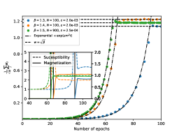
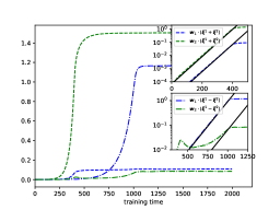
Figure 1: Learning behavior of the BG-RBM with one hidden node, using data from the CW model at different inverse temperatures, system size and learning rate $\beta,N,\epsilon$. The argument of the exponential curves is set to $m^{2}\epsilon N$, where $\epsilon$ is the learning rate. Inset: Behavior of $\chi$ along with the magnetization $h^{*}$ of the learning RBM. The vertical line marks where the susceptibility diverges, indicating the onset of spontaneous magnetization.Right: Learning curves for RBMs learning two correlated patterns. The dashed curves represent the weights of the two hidden nodes projected onto $\bm{\xi}^{1}+\bm{\xi}^{2}$, while the dashed-dot curves are projected onto $\bm{\xi}^{1}-\bm{\xi}^{2}$. Inset: Exponential growth during the two phases: top shows growth towards $\bm{\xi}^{1}+\bm{\xi}^{2}$ at a rate $r^{2}(1+\kappa)/2$, and bottom shows growth towards $\bm{\xi}^{1}-\bm{\xi}^{2}$ at a rate $p^{2}(1-\kappa)/2$. The arguments of the exponentials are not adjusted.

4.2 Learning multiple features though a cascade of phase transitions

We consider now the case in which the data are characterized by more than two features. For concreteness, we focus on the case in which the data is drawn from the probability distribution of the Hopfield model [30] with two patterns $\bm{\xi}^{1}$ and $\bm{\xi}^{2}$, using the Hamiltonian $\mathcal{H}_{H}[\bm{v}]=-\frac{\beta}{2N_{\mathrm{v}}}\sum_{\mu=1}^{2}\left(\sum_{i=1}^{N_{\mathrm{v}}}\xi_{i}^{\mu}v_{i}\right)^{2}$. The generalization to a larger number of patterns is straightforward. Following [31] we consider the case in which the patterns are correlated and defined as: $\bm{\xi}^{1}=\bm{\eta}+\bar{\bm{\eta}}$ and $\bm{\xi}^{2}=\bm{\eta}-\bar{\bm{\eta}}$; $\bm{\eta}$ is a vector whose first $N_{\mathrm{v}}\frac{1+\kappa}{2}$ components are equal to $\pm 1$ with equal probability, and the remaining ones are zero ($0<\kappa<1$). Whereas $\bar{\bm{\eta}}$ is a vector whose last $N_{\mathrm{v}}\frac{1-\kappa}{2}$ components are equal to $\pm 1$ with equal probability, and the remaining ones are zero. When $T<1-\kappa$ this model is in a symmetry broken phase in which the measure is supported by four different lumps centred in $\pm\bm{\xi}^{1}$ and $\pm\bm{\xi}^{2}$. Analogously to what was done previously, we now consider a BG-RBM with a number of hidden nodes equal to the number of patterns. The Hamiltonian is then given by $\mathcal{H}[\bm{v},\bm{h}]=-\sum_{i\mu}v_{i}h_{\mu}w_{i,\mu}+\sum_{\mu}h_{\mu}^{2}N/2$, which corresponds to a Hopfield model [30] with patterns $\bm{w}^{1}$ and $\bm{w}^{2}$. The analysis presented in the previous section can be generalized to this case (see SI for more details) and one finds the dynamical equations for the evolution of the patterns:

$$\frac{dw_{i}^{\mu}}{dt}=\frac{1}{N_{\mathrm{v}}}\sum_{j}\langle v_{i}v_{j}\rangle_{\mathcal{D}}w_{j}^{\mu}-\frac{1}{N_{\mathrm{v}}}\sum_{j}\langle v_{i}v_{j}\rangle_{\rm RBM}w_{j}^{\mu}$$ (4)

As shown in the SI C, $\langle v_{i}v_{j}\rangle_{\mathcal{D}}=r^{2}\xi_{i}\xi_{j}+p^{2}\eta_{i}\eta_{j}$ where $r,p$ are a function of $\beta$ (and $\beta^{-1}=T<1-\kappa$, $r>p$). At the beginning of the training dynamics the RBM is in its high-temperature disordered phase, hence the second term of the RHS of Eq. (4) is zero. The weights $\bm{w}^{1}$ and $\bm{w}^{2}$ have therefore an exponential growth in the directions $\bm{\eta}$ and $\bar{\bm{\eta}}$, whereas the other components do not evolve. If the initial condition for the weights is very small, as we assume for simplicity, one can then write:

$$\bm{w}^{\mu}(t)=\frac{z^{\mu}}{\sqrt{N_{\mathrm{v}}\left(\frac{1+\kappa}{2}\right)}}e^{r^{2}\left(\frac{1+\kappa}{2}\right)t}\bm{\eta}+\frac{\tilde{z}^{\mu}}{\sqrt{N_{\mathrm{v}}\left(\frac{1-\kappa}{2}\right)}}e^{p^{2}\left(\frac{1-\kappa}{2}\right)t}\bar{\bm{\eta}}\qquad\mu=1,2\,\,\,\,,$$

where we have neglected the small remaining components; $z^{\mu}$ and $\tilde{z}^{\mu}$ are the projections of the initial condition along the directions $\bm{\eta}$ and $\bar{\bm{\eta}}$. Since $r>p$, on the timescale $(\log N_{\mathrm{v}})/\left(r^{2}(1+\kappa)\right)$ the component of the $\bm{w}^{\mu}s$ along $\bm{\eta}$ becomes of order one whereas the one over $\bar{\bm{\eta}}$ is still negligible. In this regime, the RBM is just like the one we consider in the previous section with a single pattern $\bm{\eta}$, and it has a phase transition at the time $t_{I}$:

$$\frac{e^{2r^{2}\left(\frac{1+\kappa}{2}\right)t_{I}}}{N_{\mathrm{v}}}\left((z^{1})^{2}+(\tilde{z}^{1})^{2}\right)=1\,\,,$$

which is analogous to the one studied in the previous section. At $t_{I}$, the RBM learns that the data can be splitted in two groups centred in $\pm\bm{\eta}$, but it does not have yet learned that each one of these two groups consist in two lumps centred in $\bm{\xi}^{1}$ and $\bm{\xi}^{2}$ (and respectively $-\bm{\xi}^{1}$ and $-\bm{\xi}^{2}$). The training dynamics after $t_{I}$ can also be analyzed: the components of the weight vectors along $\bm{\eta}$ evolve and settle on timescales of order one to a value which is dependent on the initial condition (see the eq. in the SI). In the meanwhile, the components along $\bar{\bm{\eta}}$ keep growing; at a timescale $(\log N_{\mathrm{v}})/(p^{2}(1-k))$ (quite larger than $t_{I}$ in the limit $N_{\mathrm{v}}\to\infty$) they become of order one. In order to analyze easily this regime, let’s consider first the simple case in which the initial condition on the weights is such that $\bm{w}^{1}(0)\cdot\bar{\bm{\eta}}=-\bm{w}^{2}(0)\cdot\bar{\bm{\eta}}$ and $\bm{w}^{1}(0)\cdot\bm{\eta}=\bm{w}^{2}(0)\cdot\bm{\eta}$. In this case, one can write $\bm{w}^{1}=A(t)\bm{\eta}+B(t)\bar{\bm{\eta}}$ and $\bm{w}^{2}=A(t)\bm{\eta}-B(t)\bar{\bm{\eta}}$. The corresponding RBM is a Hopfield model with log likelihood:

$$\sum_{\mu}\frac{(\sum_{i}v_{i}w_{i}^{\mu})^{2}}{2N_{\mathrm{v}}}=2A(t)^{2}\frac{(\sum_{i}v_{i}\eta_{i})^{2}}{2N_{\mathrm{v}}}+2B(t)^{2}\frac{(\sum_{i}v_{i}\bar{\eta}_{i})^{2}}{2N_{\mathrm{v}}}$$

At $t_{I}$, when $\left(\frac{1+\kappa}{2}\right)A(t_{I})^{2}=1$, one has the first transition in which the RBM measure breaks in two lumps pointing in the direction $\pm\bm{\eta}$, as we explained above. In this regime $B(t)$ is still negligible but keeps increasing with an exponential rate. Using the results of [31], one finds that when $\frac{1-\kappa}{2}B(t_{II})^{2}=1$, a second phase transition takes place. This defines a time $t_{II}$ at which the probability measure of the RBM breaks from two lumps to four lumps, each one centred around one of the four directions $\pm\bm{\xi}^{1},\pm\bm{\xi}^{2}$. We have considered a special initial condition, but the phenomenon we found is general. In fact, for any initial condition one can show that the dynamical equations have an instability on the timescale $t_{II}$, which generically induces the second symmetry breaking transition. On Fig. 1, right panel, we illustrate the exponential growth as described by the theory, toward the two directions. In the SI 4.2, we show how these phase transitions are in very good agreement with previous work [9, 8] and how the phase space is split during training time. At the end of the training, the patterns are given by $\bm{w}^{1}=\xi^{1}$ and $\bm{w}^{2}=\xi^{2}$ modulo a rotation in the subspace spanned by $\bm{\xi}^{1,2}$, since the likelihood is invariant by rotations in this subspace. In fact, we often found that the patterns are not perfectly aligned because we are not forcing the weights to be binary. This analysis can naturally extend to more than two patterns, typically resulting in a cascade of phase transitions. In this process, the RBM progressively learns the data features, starting from a coarse-grained version (just the center of mass) and gradually refining until all patterns are learned.

5 Numerical Analysis

In the previous sections, we examined the learning process in simplified setups, in order to be able to develop an analytical treatment. We now show that the insights gained from this simplified analysis are also applicable to understanding the learning process of a Bernoulli-Bernoulli RBM (BB-RBM) trained with real data sets. For this purpose, we will consider 3 real data sets: (i) The Human Genome Dataset (HGD), (ii) MNIST and (iii) CelebA, see details in the appendix E. To show the occurrence of bonafide phase transitions, it is important to show the effect of increasing the system size (which transforms cross-overs in sharp transitions). We will therefore resize these data sets in different dimensions by adjusting their resolution, i.e. by changing $N_{\mathrm{v}}$ while maintaining comparable statistical properties. Detailed information about the scaling process can be found in the SI.

In real training processes, the machine is expected to incrementally learn various patterns, $\bm{\xi}^{\alpha}$, from the data as discussed in previous sections. However, the identification of these patterns and their relationship to the statistical properties of the dataset remain unclear. Prior research [9, 8, 32] has demonstrated that RBM training initiates with the stepwise encoding of the most significant principal components of the dataset, $\{\bm{u}_{\text{PCA}}^{\alpha}\}$, which are the eigenvectors of the sample covariance matrix with the highest eigenvalues, on the SVD decomposition of its weight matrix $W_{ia}=\sum_{\alpha}w_{\alpha}u_{i}^{\alpha}\bar{u}_{a}^{\alpha}$, where $\bm{u}^{\alpha}\in\mathbb{R}^{N_{\mathrm{v}}}$ and $\bar{\bm{u}}^{\alpha}\in\mathbb{R}^{N_{\mathrm{h}}}$ denote the left and right singular vectors corresponding to the singular value $w_{\alpha}$. These vectors form orthonormal bases in $\mathbb{R}^{N_{\mathrm{v}}}$ and $\mathbb{R}^{N_{\mathrm{h}}}$ respectively, where the index $\alpha$ ranges from 1 to $\min(N_{\mathrm{v}},N_{\mathrm{h}})$ and the singular values $w_{\alpha}$ are arranged in descending order. At the beginning of the learning process, the left singular vectors, $\bm{u}^{\alpha}$, gradually alignes $\alpha$-by-$\alpha$ to $\bm{u}_{\text{PCA}}^{\alpha}$. This is in agreement with previous results and our theoretical analysis. In the analogy with mean-field magnetic models developed in the previous section, the role of decreasing temperature is played by the increasing magnitude of the singular value $w_{\alpha}^{2}$ and should lead to a series of phase transitions in which the RBM measure splits in progressively larger components. We show in Fig. 2 that these phenomena are at play by focusing on the evolution of the SVD of the RBM weight matrix when training with the HGD dataset. In panel A we show the first two directions of the principal component analysis (PCA) of the dataset, which highlights its strong mode structure, as several distant clusters appear (they are related to the continental origin of the individuals at hand). In Fig. 2–B we show the strong increase of the singular values $w_{\alpha}$, indeed expected from our theoretical analysis, and in Fig. 2–C the evolution of the scalar product between $\bm{u}_{\alpha}$ and $\bm{u}^{\mathrm{PCA}}_{\alpha}$ as a function of the number of training epochs. Different colors indicate different values of $\alpha$. As expected, the modes are progressively expressed during training, and the first two singular vectors match the two principal directions of the dataset for a while. This last figure also shows us that the agreement with the PCA is only temporary (a limitation of current theoretical approaches), as the machine finds better patterns to encode the data as training progresses.

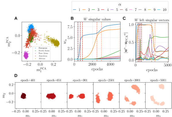
Figure 2: Human genome dataset. Progressive coding of the main directions of the dataset when training an RBM with the human genome dataset [33]. In A, we show the dataset projected along the first two principal components of the dataset $\bm{u}_{\alpha}^{\text{PCA}}$ with $\alpha=1,2$, and $m_{\alpha}^{\text{PCA}}=\bm{u}_{\alpha}^{\mathrm{PCA}}\cdot\bm{x}^{(d)}/\sqrt{N_{\mathrm{v}}}$, with $\bm{x}^{(d)}$ referring to the different entries in the dataset, i.e. an human individual. Points are colored according to the individual continental origin. In B, we show the evolution of the singular values $w_{\alpha}$ of the RBM weight matrix $\bm{W}$ as a function of the number of training epochs, and in C, we show the scalar product of the corresponding singular vectors $\bm{u}_{\alpha}$ with the corresponding PCA component $\bm{u}_{\alpha}^{\mathrm{PCA}}$. In D, we show the magnetization of the samples generated by the model at different epochs, projected along the first two eigenvectors of $\bm{W}$, which shows that the specialization of the model occurs through the progressive encoding of the main modes of the data in $\bm{W}$.

The progressive splitting of the RBM measure during the training dynamics is shown in Fig. 2–D, for which we use $N_{\mathrm{s}}=1000$ independent samples generated with the model trained up to a different number of epochs (the colors refer to the same epochs highlighted with vertical lines in Figs. 2–B and C). For visualization, we show the samples projected onto the right singular vectors of $\bm{W}$, the magnetizations $m_{\alpha}=\bm{v}\cdot\bm{u}^{\alpha}/\sqrt{N_{\mathrm{v}}}$ with $\alpha=1,2$. At the beginning of training, the data points are essentially Gaussian distributed, and the growth of $w_{1}$ over 4 is related to the splitting of the data into two different clusters on the $m_{1}$ axis, and the emergence of $w_{2}$ is related to a second splitting on the $m_{2}$ axis. The projections along all subsequent directions are Gaussian at this stage of training. This progressive splitting is crucial to express the diversity of the dataset shown in Fig. 2–A, and can be successfully used to extract relational trees from data points, as recently shown in Ref. [16]. At the beginning of training, when only one singular value has been expressed, the transition of feature encoding is analogous to the transition from the paramagnetic to the ferromagnetic phase in the aforementioned CW model. To justify this statement, we show in the SI D how, by considering the condensation of the variables onto the SVD of $\bm{W}$: $m=\bm{u}\cdot\bm{s}$, the model can be expressed as a Mattis model where the pattern is defined by $\bm{u}$. Our analysis allows us to define a temperature, linked to the eigenmode of $\bm{W}$ as $\beta=w^{2}/16$. Now, since the critical temperature of the Mattis model is $\beta_{c}=1$, we can show that the BB-RBM will condensate when the first eigenmode of the model reaches $w_{c}=4$, see SI D. In a real training, we also have visible $\bm{b}$ and hidden bias $\bm{c}$ which could easily change the model towards a random field CW model, which leads us to expect a slightly higher critical point but a very similar ferromagnetic phase transition, and in particular, it should not change the transition’s mean-field universality class.

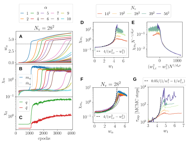
Figure 3: Traning with the MNIST dataset. In A we show the evolution of the singular values of the RBM’s coupling matrix $\bm{W}$ as a function of the training time. In $B$ we show the evolution of the susceptibilities associated with the magnetizations along the right singular vectors of $\bm{W}$, $m_{\alpha}=\left\langle\bm{u}_{\alpha}\cdot\bm{x}\right\rangle/N_{\mathrm{v}}$. In both figures, we consider the standard $N_{\mathrm{v}}=28^{2}$ MNIST dataset, different colors refer to different modes. In C we show the susceptibility associated with the overlaps $q$ and $\bar{q}$ between visible and hidden variables. In D we show the susceptibility of the first mode as a function of the first singular value $w_{1}$ obtained with trainings on MNIST data scaled to different system sizes above and below $L=28$. The numerical curves are compared with the theoretical expectation using the CW model in Eq. (6) using $w_{1,\mathrm{c}}=4.45$. The same data are shown in E, scaled using the mean-field finite-size scaling ansatz of Eq. (7). In F, we show the first 10 modes’ susceptibilities $\chi_{m_{\alpha}}$ as a function of their corresponding singular value $w_{\alpha}$ and compare them with the theoretical curve in D. In G, we show the MCMC relaxation time of the machines trained with different $N_{\mathrm{v}}$ datasets as a function of $w_{1}$, together with the theoretical expectation for local moves in dashed lines.

In order to show the existence of a cascade of transitions, and that what found for the HGD also holds for other datasets, we now train the RBM on the MNIST dataset. In Fig. 3–A we present the evolution of the singular values $w_{\alpha}$ along the training which neatly show the progressive encoding of patterns. The progressive splitting of the RBM measure in clusters and the existence of a phase transition can be monitored by measuring the variance of the distribution of the visible magnetizations $m_{\alpha}$ along the $\alpha$-th mode, or the analogous hidden magnetizations $\bar{m}_{\alpha}=\bm{h}\cdot\bar{\bm{u}}^{\alpha}/\sqrt{N_{\mathrm{h}}}$ obtained using the hidden units. The variance of the magnetization multiplied by the number of variables used to compute it and $\beta$, is related with the magnetic susceptibility via the fluctuation dissipation theorem, which means that

$$\chi_{m}=N_{\mathrm{v}}\left({\left\langle m^{2}\right\rangle-\left\langle m\right\rangle^{2}}\right)=T\frac{d\left\langle m\right\rangle}{dh},$$ (5)

here $\left\langle\cdot\right\rangle$ refers to the equilibrium measure with respect to RBM’s Gibbs measure $p(\bm{v},\bm{h})$, in practice estimated as the average over $N_{\mathrm{s}}$ independent MCMC runs. It is well known that the magnetic susceptibility should diverge in the vicinity of a second order phase transition and that such growth in only limited by the overall system size $N=\sqrt{N_{\mathrm{v}}N_{\mathrm{h}}}$ in finite systems. These phenomena indeed takes place also in the RBM. We show in Fig. 3–B the evolution of the $\chi_{m}$s obtained using the magnetizations obtained along the different modes $\alpha$ of $\bm{W}$. As anticipated, the first mode’s susceptibility sharply grows as $w_{1}$ approaches 4, but it is more remarkable that this behavior is not only restricted to the first mode, but it is also reproduced by the subsequent modes in a step-wise process. According to the mapping between the low-rank RBM and the CW model, we should expect that our $\chi_{m}$, at least for the first mode $\alpha=1$ should behave as

$$\chi_{m}\sim\frac{4}{\beta_{\mathrm{c}}-\beta}=\frac{4}{w_{\mathrm{c}}^{2}-w^{2}},$$ (6)

when approaching the critical point, which is equivalent to stating that $\gamma=1$. Here, the factor 4 in the numerator is related to the fact that the susceptibility obtained with $\{0,1\}$ variables is 4 times the standard one obtained with Ising spins, and the fact that $\beta=w^{2}/16$. In Fig. 3–D, we show the first susceptibility as a function of $w_{1}$ using RBMs trained with MNIST data rescaled to different dimensions. As mentioned before, the growth of the susceptibility is limited by the system size $N_{\mathrm{v}}$. But, as we look into larger and larger sizes, we are able to observe the growth over more decades showing that at the transition we observe the CW expected behavior of Eq. 6 as shown in black dashed line, where the only adjustable parameter was the critical point $w_{\mathrm{1,c}}=4.4$ (i.e. there is no adjustable prefactor).

One of the crucial tests to ensure that a finite-size transition is a bona fide phase transition is to study its behavior by changing the number of degrees of freedom. One of the standard tools to do this this is to make use of the so-called finite-size scaling (FSS) ansatz, motivated by renormalization group arguments [34, 35, 36]. Mean-field models follow a standard FSS ansatz which has been first studied in [37]. In particular, the FSS ansatz for the susceptibility is

$$\chi^{N}_{m}(\beta)=N^{\frac{\gamma}{\nu d_{\mathrm{u}}}}\phi\left({N^{\frac{1}{\nu d_{u}}}|\beta-\beta_{\mathrm{c}}|}\right),$$ (7)

with $\phi(\cdot)$ a size-independent scaling function, $N=\sqrt{N_{\mathrm{v}}N_{\mathrm{h}}}$ is the effective size of our model and $\gamma=1$, $\nu=1/2$ and $d_{u}=4$ as expected in the mean-field universality class. We test this ansatz in Fig. 3–E showing that it does succeed to scale the finite-size data in the critical region, especially in the largest system sizes, which confirms both the mean-field universality class and the prevalence of the transition in the thermodynamic limit. In Fig. 4-A and B, and Fig. 4-C and D, we show that the indicators of a phase transitions–growth of the susceptibility and its mean-field finite size scaling–also holds for CelebA and HGD datasets. Finally, a final piece of evidence of the existence of a phase transition is presented in Fig. 4-E, where we show that after the continous transition has taken place, one can induce a discontinuous transition and hysteresis by applying a field in the direction of the learned pattern, in full agreement with what observed for standard phase transitions.

All this previous discussion concerned mostly the first phase transition when the RBM learns the first mode. But we discussed in Fig. 3–B that an entire sequence of step-wise phase transitions occurred in the rest of the $\bm{W}$-matrix modes. In Fig. 3–F, we show each of these mode susceptibilities $\chi_{m_{\alpha}}$ as a function of their corresponding singular value, showing an extremely similar diverging behavior with respect to mode $\alpha=1$, with an apparent slight variation of the critical point for each mode though all seem to remain nearby the predicted $w_{\alpha}\sim 4$, suggesting that the subsequent transitions might be of similar mean-field nature. The crossing of second order phase transitions have very strong consequences in the overall quality of the training, in particular, with the quality of the log-likelihood gradient estimated via MCMC dynamics. Indeed, second order transitions are associated with a well known arrest effect known as critical slowing-down behavior, by which the thermalization times diverge with the correlation length $\xi^{z}\propto|\beta-\beta_{\mathrm{c}}|^{-\nu z}$, with $z$ the dynamical critical exponent which for local and non-conserved order parameter moves is 2 in mean-field, thus making large systems extremely challenging to thermalize in practice. We show that our exponential relaxation times diverges exactly as predicted in Fig. 3–G.

6 Conclusions

In this work, we first characterized the learning mechanism of RBMs using a simplified context with a dataset provided by a simple teacher model. We used two examples: one with two symmetric clusters and another with four correlated clusters. Our results show that the learning dynamics identify modes by exponential growth in the directions of the clusters, dominated by the variances of these clusters. The theory predicts the timing of the first phase transitions, aligning well with [8]. Numerically, we confirmed the existence of a cascade of phase transitions linked to the growing modes $w_{\alpha}$ and associated with diverging susceptibility. Finite-size scaling indicates these transitions are critical and in the mean-field universality class. This series of phase transitions likely extends beyond RBMs, offering insights into learning mechanisms, especially for generative models. These transitions have significant implications for both training and understanding learned features. During training, each transition is linked to a diverging MCMC relaxation time, requiring careful handling to train the model properly. Additionally, the hysteresis phenomenon ensures that the learning trajectory involves second-order phase transitions, which are beneficial for tracking the creation of modes in the learned distribution. However, altering parameters (such as local bias) could lead to first-order transitions, which are detrimental for sampling and may explain the inefficacy of parallel tempering with temperature changes. Practically, our analysis shows that the principal directions of the weight matrix contain valuable information for understanding the learned model.

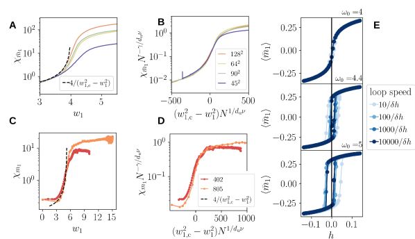
Figure 4: Traning with the CELEBA and HGD datasets. In A, for the CELEBA dataset, we plot the hidden susceptibility for different system sizes. In dashed lines we show the expected divergence for $w_{1,c}=4$. In B, the mean-field FFS associated with the first transition using the mean-field exponents. In C and D, we repeat show the visible susceptibility associated to the first phase transition in the HGD. In this case, we use $w_{1,c}=5.25$ for the scalings. In E, we illustrate the typical hysteresis behavior in low-temperature phase, similar to what is observed in mean-field Ising model in fields.

7 acknowledgments

The authors would like to thank J. Moreno-Gordo for his work and discussions during the initial phase of this project. The authors ( A.D. and B.S.) acknowledge financial support by the Comunidad de Madrid and the Complutense University of Madrid (UCM) through the Atracción de Talento program (Refs. 2019-T1/TIC-13298), and to project PID2021-125506NA-I00 financed by the Ministerio de Economía y Competitividad, Agencia Estatal de Investigación (MICIU/AEI /10.13039/501100011033), and the Fondo Europeo de Desarrollo Regional (FEDER, UE).

Appendix A Binary-Gauss RBM

We add some technical details to the derivation of the dynamical process. Recall that we consider the CW model, biased toward a pattern $\bm{\xi}$ for generating the dataset

$$p_{CW}(\bm{v})=\frac{1}{Z_{CW}}\exp\left(\frac{\beta}{2N_{\mathrm{v}}}\left(\sum_{i=1}^{N_{\mathrm{v}}}\xi_{i}v_{i}\right)^{2}\right)$$

where $\beta$ is the inverse temperature $\beta=1/T$ and $\xi_{i}s=\pm 1$ represents a potential pattern direction. The CW model presents a high-temperature phase with a single model centred over zero magnetization $m=N^{-1}_{N_{\mathrm{v}}}\sum_{i}s_{i}=0$ for $\beta<\beta_{c}$ while in the low-temperature regime, $\beta>\beta_{c}$, the model exhibits a phase transition between two symmetric modes $m=\pm m_{0}(\beta)$. From the analytical point of view, we can compute all interesting quantities in the thermodynamics limit $N_{\mathrm{v}}\to\infty$. The RBM’s distribution is given by

$$p_{RBM}(\bm{h},\bm{v}) =\frac{1}{Z_{RBM}}\exp\left(\sum_{i}v_{i}hw_{i}-\frac{h^{2}N}{2}\right)$$

$$p_{RBM}(\bm{v}) =\frac{1}{Z}\exp\left(\frac{(\sum_{i}v_{i}w_{i})^{2}}{2N_{\mathrm{v}}}\right)$$

Using this model for the learning, the time evolution of the weights is given by the gradient. With binary-Gaussian RBM we have that

$$\langle v_{i}h\rangle =\sum_{\{\bm{v}\}}\int dhv_{i}hp(\bm{v},h)=\sum_{\{\bm{v}\}}\int dhv_{i}hp(h|\bm{v})p(\bm{v})$$ (8)

$$=\frac{1}{N}\sum_{\{\bm{v}\}}v_{i}\sum_{j}v_{j}p(\bm{v})w_{j}=\frac{1}{N}\sum_{j}w_{j}\langle v_{i}v_{j}\rangle_{p}$$ (9)

where the last average is taken over a distribution $p(\bm{v})$. We can now easily compute the positive and negative term of the gradient w.r.t. the weight matrix. For the positive term, assuming that $\beta>1$, we obtain that

$$\langle v_{i}v_{j}\rangle_{\mathcal{D}} =\frac{1}{Z_{CW}}\int dm\sum_{\{\bm{v}\}}v_{i}v_{j}\exp\left(-\beta N_{\mathrm{v}}\frac{m^{2}}{2}+\beta\sum_{i}\xi_{i}v_{i}\right)$$

$$=\frac{1}{Z_{CW}}\int dm\tanh(\beta\xi_{i}m)\tanh(\beta\xi_{j}m)\exp\left(-\beta N_{\mathrm{v}}\frac{m^{2}}{2}+\sum_{i}\log 2\cosh(\beta\xi_{i}m)\right)$$

Evaluating the saddle point of the argument of the exponential (which is the same as the one for the partition function) we have that

$$\langle v_{i}v_{j}\rangle_{\mathcal{D}}=\xi_{i}\xi_{j}m^{2}\text{ where }m=\tanh\left(\beta m\right)$$

The negative term can also be computed in the thermodynamic limit

$$\langle v_{i}v_{j}\rangle_{\rm RBM} =\frac{1}{Z_{\rm RBM}}\int dh\sum_{\bm{v}}v_{i}v_{j}\exp\left(\sum_{i}v_{i}hw_{i}-\frac{h^{2}N}{2}\right)$$

$$=\int dh\frac{1}{Z_{\rm RBM}}\tanh(hw_{i})\tanh(hw_{j})\exp\left(\sum_{i}\log\left[2\cosh(hw_{i})\right]-\frac{h^{2}N}{2}\right)$$

$$=\tanh(h^{*}w_{i})\tanh(h^{*}w_{j})\text{ with }h^{*}=\frac{1}{N}\sum_{k}w_{k}\tanh(h^{*}w_{k})$$

where the last line is obtain by taking the saddle point of the integral over $h$, ($h^{*}$ corresponding to the extremum). We can now express the gradient as

$$\frac{dw_{i}}{dt}=\frac{1}{N}\xi_{i}\sum_{k}\xi_{k}w_{k}m^{2}-\sum_{k}w_{k}h^{*}\tanh(h^{*}w_{i})$$ (10)

Assuming first that the weights are small we get that $h^{*}=0$. We can solve the gradient’s equations in this regime. In such case, the only solution for the saddle point equation of the RBM is given by $h^{*}=0$ and we can see that the solution of the evolution of the weight is global toward the direction $\bm{\xi}$ by projecting the differential equation on the preferred direction. Defining $U_{\bm{\xi}}=N^{-1/2}\sum_{i}\xi_{i}w_{i}$, we obtain

$$\frac{dU_{\bm{\xi}}}{dt}=m^{2}U_{\bm{\xi}}\text{ thus }U_{\bm{\xi}}=U_{\bm{\xi}}^{0}e^{m^{2}t}.$$

This show that the weights are growing in the direction of $\bm{\xi}$ while the projection on any orthogonal direction $\bm{\phi}^{\alpha}$ stays constant:

$$\bm{\phi}^{\alpha}\cdot\frac{d\bm{w}}{dt}=\frac{m^{2}}{N}(\bm{\phi}^{\alpha}\cdot\bm{\xi})(\bm{w}\cdot\bm{\xi})=0\text{ since }\bm{\phi}^{\alpha}\cdot\bm{\xi}=0$$

When the weights grow larger, the solution for $h^{*}$ will depart from zero. The correlation of the learning RBM then starts to grow

$$\langle s_{i}s_{j}\rangle_{\rm RBM} \approx\frac{1}{Z}\int dhh^{2}w_{i}w_{j}\exp\left(-\frac{Nh^{2}}{2}+\sum_{i}\frac{h^{2}w_{i}^{2}}{2}\right)=w_{i}w_{j}\frac{1}{N\left(1-\sum_{i}w_{i}^{2}/N\right)}$$

$$\chi =\sum_{i,j}\xi_{j}\xi_{i}\langle s_{i}s_{j}\rangle_{\rm RBM}\approx\left(\sum_{i}\xi_{i}w_{i}\right)^{2}\frac{1}{N\left(1-\sum_{i}w_{i}^{2}/N\right)}$$

and diverges when $N^{-1}\sum_{i}w_{i}\sim 1$, therefore exhibiting a second order phase transition during the learning. Finally, we can study the regime where the weights are not small. In that case, we can first observe that the evolution of the directions orthogonal to $\bm{\xi}$, $\bm{\phi}^{\alpha}$ are given by

$$\sum_{i}\phi_{i}^{\alpha}\frac{dw_{i}}{dt}=\frac{m^{2}}{N}\sum_{i}\phi_{i}^{\alpha}\xi_{i}\sum_{k}\xi_{k}w_{k}-\sum_{i}\phi_{i}^{\alpha}h^{*}\tanh(h^{*}w_{i})=-\sum_{i}\phi_{i}^{\alpha}h^{*}\tanh(h^{*}w_{i})$$

which will cancel if the weight $\bm{W}$ aligns totally with the $\bm{\xi}$. Finally, taking $w_{i}=\xi_{i}w,$ the gradient projected along $\bm{\xi}$ at stationarity imposes

$$wm^{2}=h^{*}\tanh^{2}(h^{*}w)\text{ and thus }w=\sqrt{\beta}\text{ and }h^{*}=\sqrt{\beta m}$$

Appendix B Binary-Binary RBM

The RBM sharing both discrete binary variables on the visible and hidden nodes is by far the mostly commonly used. In particular, using binary nodes in the hidden layer instead of the Gaussian distribution allow the model to potentially fit any order correlations of the dataset. In this section, we review how the learning dynamics translate to this case, using for simplicity binary $\{\pm 1\}$ variables. In order to obtain an interesting behavior in this phase of the learning, it is important to consider a particular parametrization of the RBM. We consider that all hidden nodes share the same weight. This is important to be able to have a recall phase transition in the model. We therefore have the following Hamiltonian

$$\mathcal{H}=-\frac{1}{N_{\mathrm{h}}}\sum_{i}s_{i}w_{i}\sum_{a}\tau_{a}$$ (11)

where $N_{\mathrm{h}}=\alpha N$ is the number of hidden nodes $\tau_{a}$ of the system and the vector $\bm{W}$ correspond to the weight shared across all the hidden nodes. In this model, we can now compute the positive and negative of the gradient. The first one is given by

$$\frac{1}{N_{h}}\langle s_{i} \sum_{a}h_{a}\rangle_{\mathcal{D}}=\frac{1}{Z_{CW}}\sum_{\bm{s}}\int dms_{i}\exp\left(-\frac{\beta m^{2}N}{2}+m\beta\sum_{j}\xi_{j}s_{j}\right)\frac{1}{N_{\mathrm{h}}}\sum_{a}\tanh\left[N_{\mathrm{h}}^{-1}\sum_{j}w_{j}s_{j}\right]$$

$$=\frac{1}{Z_{CW}}\sum_{\bm{s}}\int dmd\tau s_{i}\exp\left(-\frac{\beta m^{2}N}{2}+m\beta\sum_{j}\xi_{j}s_{j}\right)\delta(\tau-N_{\mathrm{h}}^{-1}\sum_{j}w_{j}s_{j})\tanh(\tau)$$

$$=\frac{1}{Z_{CW}}\sum_{\bm{s}}\int d\tau d\bar{\tau}dms_{i}\exp\left(-\frac{\beta m^{2}N}{2}+m\beta\sum_{j}\xi_{j}s_{j}\right)\tanh(\tau)e^{i\tau\bar{\tau}-iN_{\mathrm{h}}^{-1}\bar{\tau}\sum_{j}w_{j}s_{j}}$$

$$=\frac{1}{Z_{CW}}\sum_{\bm{s}}\int dmd\tau d\bar{\tau}e^{-\beta m^{2}N/2+i\tau\bar{\tau}}\tanh(\xi_{i}m\beta-iN_{\mathrm{h}}^{-1}\bar{\tau}w_{i})\tanh(\tau)$$

$$\;\;\;\;\;\;\;\;\;\;\;\;\times\exp\left(\sum_{j}\log\cosh\left[\xi_{j}\beta m-iN_{\mathrm{h}}^{-1}\bar{\tau}w_{j}\right]\right)$$

finding the saddle point of the argument in the exponential, we obtain

$$\frac{1}{N_{h}}\langle s_{i}\sum_{a}h_{a}\rangle_{\mathcal{D}}=\xi_{i}\tanh(\beta m)\tanh\left(\frac{m}{N_{\mathrm{h}}}\sum_{j}\xi_{j}w_{j}\right)=\xi_{i}m\tanh\left(\frac{m}{N_{\mathrm{h}}}\sum_{j}\xi_{j}w_{j}\right)$$

The same type of computation can be done for the negative term, we found that

$$\frac{1}{N_{h}}\langle s_{i}\sum_{a}h_{a}\rangle_{RBM} =\xi_{i}\tau\tanh\left(w_{i}\tau\right)$$

$$\tau =\tanh\left(\frac{1}{N_{h}}\sum_{j}w_{j}\tanh\left(w_{j}\tau\right)\right)$$

Again, in the small coupling regime (or at the beginning of the learning), when $N_{\mathrm{h}}^{-1}\sum_{j}w_{j}^{2}\ll 1$, we have that $\tau=0$. In such case, the gradient over the weight matrix is given by

$$\frac{dw_{i}}{dt}=\xi_{i}m\tanh\left(\frac{m}{N_{\mathrm{h}}}\sum_{j}\xi_{j}w_{j}\right)$$

following the same approach as in the main text, we project the weights on the unit vector $\bm{u}_{1}=\bm{\xi}/\sqrt{N}$, $U_{\bm{\xi}}=\bm{u}_{1}\bm{W}$, which gives

$$\frac{dU_{\bm{\xi}}}{dt}=\sqrt{N}m\tanh\left(\frac{m\sqrt{N}}{N_{\mathrm{h}}}U_{\bm{\xi}}\right)$$

We can integrate this equation, obtaining the solution

$$\sinh\left(\frac{m}{\sqrt{N}\alpha}U_{\bm{\xi}}(t)\right) =\sinh\left(\frac{m}{\sqrt{N}\alpha}U_{\bm{\xi}}(0)\right)\exp\left(\frac{m^{2}t}{\alpha}\right)$$

$$U_{\bm{\xi}}(t) =U_{\bm{\xi}}(0)\exp\left(\frac{m^{2}t}{\alpha}\right)$$

where the second line is obtained in the very large $N$ limit. Again we have an exponential growth in the first steps of the learning. At the end of the learning, the weights again align in the direction of $\bm{\xi}$. This can be checked by the fact that the positive term of always orthogonal to any vector orthogonal to $\bm{\xi}$, and thus the simplest option for the gradient projected in those direction is to be orthogonal to $\bm{\xi}$. Taking $\bm{W}=\bm{u}_{1}w$, we obtain

$$m\tanh\left(mw/\alpha\right) =\tau\tanh(w\tau)$$

$$\tau =\tanh(w\tanh(w\tau)/\alpha)$$

The solution can be found numerically by solving the fixed point equation on $\tau$, and measuring the magnetization of the dataset. In Fig.5 we illustrate our results in the same dataset as in the section 4.1, taking the CW model with $N=900$, $\beta=1.4$, varying the learning rate and the number of hidden nodes.

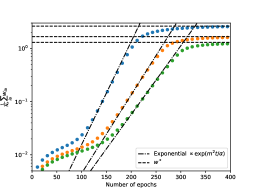
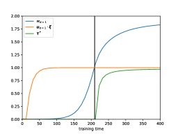
Figure 5: Left: learning behavior of the Binary-Binary RBM, using data from the CW model. The different curves correspond to systems of size $N=900$ at inverse temperature $\beta=1.4$ with learning rate $\eta=0.03,0.04,0.05$ and $N_{\mathrm{h}}=400,700,1000$ respectively. The argument of the exponential curves are not adjusted but set to $m^{2}\eta/\alpha$. Right: we illustrate the RBM’s dynamics in the binary-binary case with $\beta=1.4$ and $N_{\mathrm{v}}=900$, $N_{\mathrm{h}}=400$. First the eigenvector $\bm{u}^{\alpha=1}$ aligns itself with the pattern $\bm{\xi}$. Then, the eigenvalue $w_{\alpha=1}$ grows exponentially until reaching saturation and when it crosses the value $1$, the system develops a spontaneous magnetization.

Appendix C Learning with correlated patterns

In this part we detail how the learning goes when considering a pair of correlated patterns. As described in 4.2, the pairs of patterns are defined as

$$\bm{\xi}^{1}=\bm{\eta}+\bar{\bm{\eta}}\text{ and }\bm{\xi}^{2}=\bm{\eta}-\bar{\bm{\eta}}$$

where $\bm{\eta}$ is a vector whose first $N_{\mathrm{v}}\frac{1+\kappa}{2}$ components are equal to $\pm 1$ with equal probability and the remaining ones are zero. The other vector $\bar{\bm{\eta}}$ has its last $N_{\mathrm{v}}\frac{1-\kappa}{2}$ components equal to $\pm 1$ with equal probability and the rest are 0; we also have that $\kappa\in[0,1]$. When $\kappa=1$, both patterns $\bm{xi}^{1,2}$ are equal, while otherwise different but correlated. In particular $\mathbb{E}_{\bm{\eta},\bar{\bm{\eta}}}[\bm{\xi}^{1}\bm{\xi}^{2}]=N_{\mathrm{v}}\kappa$. Following the results of [31], it is possible to compute the saddle point equations for the magnetization. The general form is given by

$$m_{1} =\frac{1}{N_{\mathrm{v}}}\sum_{i}\xi^{1}_{i}\tanh\left(\beta m_{1}\xi^{1}_{i}+\beta m_{2}\xi^{2}_{i}\right)$$

$$m_{2} =\frac{1}{N_{\mathrm{v}}}\sum_{i}\xi^{2}_{i}\tanh\left(\beta m_{1}\xi^{1}_{i}+\beta m_{2}\xi^{2}_{i}\right)$$

This system has been solved in [31] and exhibits the following properties. When $T>1+\kappa$, the system is in the paramagnetic regime and $m_{1}=m_{2}=0$. When the temperature is lowered and lies in $1-\kappa<T<1+\kappa$, the solution is given by the pair retrieval $m_{1}=m_{2}=m=\frac{1+\kappa}{2}\tanh(2\beta m)$. Finally, when $T<1-\kappa$, the system condensate on the following solution

$$m_{1} =\frac{1+\kappa}{2}\tanh\left(\beta(m_{1}+m_{2})\right)+\frac{1-\kappa}{2}\tanh\left(\beta(m_{1}-m_{2})\right)$$

$$m_{2} =\frac{1+\kappa}{2}\tanh\left(\beta(m_{1}+m_{2})\right)-\frac{1-\kappa}{2}\tanh\left(\beta(m_{1}-m_{2})\right)$$

where basically the system either condensate toward one of the pattern $\bm{\xi}^{1,2}$, while the other magnetization has some non-zero value due to the correlation.

We can use the thermodynamics properties of this model to study how the learning of the RBM should behave in the regime $T<1-\kappa$. In order to use this model as generating the dataset, we need to compute the correlations $\langle s_{i}s_{j}\rangle$. The model present four fixed point, all equally probable:

$$(m_{1},m_{2}) =(m^{+},m^{-})\text{ and its symmetric case }(m_{1},m_{2})=(-m^{+},-m^{-})$$

$$(m_{1},m_{2}) =(m^{-},m^{+})\text{ and its symmetric case }(m_{1},m_{2})=(-m^{-},-m^{+})$$

where $m^{+}>m^{-}>0$. Therefore, write $r=\tanh(\beta(m^{+}+m^{-}))$ and $p=\tanh(\beta(m^{+}-m^{-}))$ we have that

$$\langle s_{i}s_{j}\rangle_{data} =\frac{1}{4}\left(\sum_{(m_{1},m_{2})}\left[(\eta_{i}+\bar{\eta}_{i})\tanh(\beta(m_{1}+m_{2}))\right]\left[(\eta_{j}+\bar{\eta}_{j})\tanh(\beta(m_{1}+m_{2}))\right]\right)$$

$$=\eta_{i}\eta_{j}r^{2}+\bar{\eta}_{i}\bar{\eta}_{j}p^{2}$$

because the cross terms $\eta_{i}\bar{\eta}_{j}$ are canceled between when changing $(m_{1}=m^{+},m_{2}=m^{-})$ to $(m_{1}=m^{-},m_{2}=m^{+})$. At this point, it is possible to write the gradient at the linear order and project it toward both direction $\bm{\eta}$ and $\bar{\bm{\eta}}$. Denoting $U_{\bm{\eta}}^{\mu}=\bm{\eta}\cdot\bm{w}^{\mu}$ and $U_{\bar{\bm{\eta}}}^{\mu}=\bar{\bm{\eta}}\cdot\bm{w}^{\mu}$, we get

$$\frac{dU_{\bm{\eta}}^{\mu}}{dt} =r^{2}\frac{1+\kappa}{2}\sum_{j}U_{\bm{\eta}}^{\mu}$$

$$\frac{dU_{\bar{\bm{\eta}}}^{\mu}}{dt} =p^{2}\frac{1-\kappa}{2}\sum_{j}U_{\bar{\bm{\eta}}}^{\mu}$$

Using this form, we end up with the following solution of the weight matrix

$$w_{i}^{\mu}(t)=w_{i}^{\mu}(0)+\frac{\eta_{i}U_{\bm{\eta}}^{\mu}(0)}{(1+\kappa)/2}\left[\exp\left(r^{2}\frac{1+\kappa}{2}t\right)-1\right]+\frac{\eta_{i}U_{\bar{\bm{\eta}}}^{\mu}(0)}{(1-\kappa)/2}\left[\exp\left(p^{2}\frac{1-\kappa}{2}t\right)-1\right]$$ (12)

We therefore understand the following. At the beginning of the learning, since $r>p$, what is learned first is the mode toward the direction $\bm{\eta}\propto\bm{\xi}^{1}+\bm{\xi}^{2}$, in a timescale that is given by time $t\sim 1/r^{2}$. At a different timescale, the part that is aligned with $\bar{\bm{\eta}}$ will grow as well as discussed in the main text. Following the dynamics of the weights, as in eq. 12, we can infer the moment where the phase transition occurs. When considering an Hopfield like model, we know that the transition happens when

$$\frac{\beta}{2N_{\mathrm{v}}}\left(\sum_{i}v_{i}\xi_{i}\right)^{2}\sim\frac{1}{2N_{\mathrm{v}}}\left(\sum_{i}v_{i}\xi_{i}\right)^{2}$$

that is, the critical temperature is $\beta_{c}=1$. Following the dynamics of the weights of eq. 12, and neglecting the terms that are not aligned with $\bm{\eta}$ we can write

$$\frac{1}{2N_{\mathrm{v}}}\left(\sum_{i}v_{i}\xi_{i}\right)^{2} \sim\left(\frac{U_{\bm{\eta}}^{\mu}(0)}{(1+\kappa)/2}\right)^{2}\left[\exp\left(r^{2}\frac{1+\kappa}{2}t\right)-1\right]^{2}\frac{1}{2N_{\mathrm{v}}}\left(\sum_{i}v_{i}\eta_{i}\right)^{2}$$

$$\beta_{\bm{\eta}}(t) =\left(\frac{U_{\bm{\eta}}^{\mu}(0)}{(1+\kappa)/2}\right)^{2}\left[\exp\left(r^{2}\frac{1+\kappa}{2}t\right)-1\right]^{2}$$

where we can identify a sort of dynamical temperature associated to the pattern $\bm{\eta}$. Now, we need to be careful since by definition, the pattern $\bm{\eta}$ is made of random $\pm 1$ components on its $(1+\kappa)/2$ elements and zero elsewhere. This rescales the critical temperature by a factor $(1+\kappa)/2$. Therefore we need to look when

$$\frac{1+\kappa}{2}\beta_{\bm{\eta}}(t_{I})\sim 1$$

and the same kind of argument can be used for the second transition with this time

$$\beta_{\bar{\bm{\eta}}}(t) =\left(\frac{U_{\bar{\bm{\eta}}}^{\mu}(0)}{(1-\kappa)/2}\right)^{2}\left[\exp\left(p^{2}\frac{1-\kappa}{2}t\right)-1\right]^{2}$$

$$\frac{1-\kappa}{2}\beta_{\bar{\bm{\eta}}}(t_{II}) \sim 1$$

We show in Fig. 6, left panel how the times $t_{I}$ and $t_{II}$ compare with the moment where the eigenvalues $w_{\alpha}$ of the weight matrix cross the value one, which correspond to the phase transition following a statistical mechanics approach [8]. We observe that both indicators are crossing the line $y=1$ at the same moment. In Fig. 6, right panel, we plot the behavior of the free energy (in the plane $(h_{1},h_{2})$). We see that at the moment of the transition, the free energy opens in the direction corresponding to the transition. Projecting the dataset (black dots) in the same direction as $h1$ (resp. $h2$), we can see how the system correctly positioned the minima once fully trained.

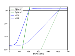
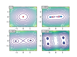
Figure 6: Left: the empirical dynamics of the eigenvalues of the weight matrix, here denotes $\tilde{w}_{\alpha}$ in blue. In green, the predicted dynamics as in eq. 12, adjusting only the initial conditions $U_{\bm{\eta}}^{\mu}(0)$ and $U_{\bar{\bm{\eta}}}^{\mu}(0)$. We see that the curves cross the line $y=1$ at the same moments $t_{I}$ and $t_{II}$. Right: the free energy in the plane $(h_{1},h_{2})$, the order parameters of the model. For different value of the weights during learning, we reconstruct the free energy of the system. We clearly see how the RBM first creates two minima, in the direction of $\bm{\eta}$, and then, split again to obtain the four fixed points.

Appendix D Link between the low-rank RBM and Mattis model

Let us consider a low-rank Ising-Ising RBM in which the $\mathcal{\bm{W}}$ matrix has a single non-zero singular value $\omega$, with left and right singular vectors $\bm{u}$ and $\bar{\bm{u}}$, and visible and hidden Ising variables (let’s call these variables $\mathcal{W}$, $\bm{s}$ and $\bm{\tau}$ to distinguish them from the binary ${0,1}$ version, which would be $\bm{W}$ and $\bm{v}$ and $\bm{h}$). In this case, the energy function of the RBM (if we ignore the biases for now) is

$$E(\bm{v},\bm{h})=-\omega(\bm{u}\cdot\bm{v})(\bar{\bm{u}}\cdot\bm{h}),$$

which leads to a marginal energy on the visible

$$\mathcal{E}(\bm{s})=-\sum_{a}\log\cosh\left[{\sqrt{N_{\mathrm{v}}}w\bar{u}_{a}^{2}m}\right]\approx-\frac{1}{2}N\omega^{2}m^{2}+O(m^{4}),$$ (13)

where we have defined $m=\bm{u}\cdot\bm{s}/\sqrt{N_{\mathrm{v}}}$ as the magnetization of the spins along the direction $\bm{u}$ and have exploited the fact that $\sum_{a}\bar{u}_{a}^{2}=1$ because it is a unit vector. One can obtain an analogous expression for the marginal energy on the hidden units, formulated in terms of the hidden magnetization $\bar{m}=\bar{\bm{u}}\cdot\bm{\tau}/\sqrt{N_{\mathrm{h}}}$. These energy functions, for small $m$ or $\bar{m}$, are formally equal to those of the CW model for $\beta=\omega^{2}$, which means that our RBM should suffer a critical phase transition at $\beta_{\mathrm{c}}=T_{\mathrm{c}}^{-1}=\omega_{\mathrm{c}}^{2}=1$, with mean-field critical exponents. Standard RBMs are not formulated as Ising $\pm 1$ variables, but in the form of binary $\{0,1\}$ variables where we have the equivalence $4\bm{\mathcal{W}}=\bm{W}$ between the couplings matrices. This results in a critical point at $w_{\mathrm{c}}=4$ and an effective inverse temperature $\beta=w^{2}/16$.

Appendix E The datasets and the rescaling

In this work, we illustrated our results on three datasets:

1. The Human Genome Dataset (HGD)  [33] containing binary vectors, each representing a selection of $805$ genes from a human individual, where 1s or 0s indicate the presence or absence of gene mutations relative to a reference sequence.

2. The MNIST dataset [38], containing $28\times 28$ pixel black and white images of digitized handwritten digits.

3. The CelebA [39] dataset, in black-and-white, with $128\!\times\!128$ pixel images of celebrities faces.

The datasets MNIST and CELEBA, were either downscaled or upscaled in order to create dataset of various sizes. In practice, the function resize from the python library skimage was used either to increase or decrease the image size. The dataset HGD is geometrically a one-dimensional structure. In order to reduce its size, we took the convolution of each sample with a kernel of size $s=3$. The output is one if the sum of the three input values (that are discrete variables in $\{0,1\}$) of the kernel is above the threshold 2 and zero otherwise. A stride of $2$ has been chosen such that the resulting samples has its size reduced by a factor two.

References

- [1] Christian Ledig, Lucas Theis, Ferenc Huszár, Jose Caballero, Andrew Cunningham, Alejandro Acosta, Andrew Aitken, Alykhan Tejani, Johannes Totz, Zehan Wang, et al. Photo-realistic single image super-resolution using a generative adversarial network. In Proceedings of the IEEE conference on computer vision and pattern recognition, pages 4681–4690, 2017.
- [2] Yilun Du and Igor Mordatch. Implicit generation and modeling with energy based models. Advances in Neural Information Processing Systems, 32, 2019.
- [3] Prafulla Dhariwal and Alexander Nichol. Diffusion models beat gans on image synthesis. Advances in neural information processing systems, 34:8780–8794, 2021.
- [4] Yann LeCun, Sumit Chopra, Raia Hadsell, M Ranzato, and Fujie Huang. A tutorial on energy-based learning. Predicting structured data, 1(0), 2006.
- [5] Diederik P Kingma and Max Welling. Auto-encoding variational bayes. arXiv preprint arXiv:1312.6114, 2013.
- [6] Ian Goodfellow, Jean Pouget-Abadie, Mehdi Mirza, Bing Xu, David Warde-Farley, Sherjil Ozair, Aaron Courville, and Yoshua Bengio. Generative adversarial networks. Communications of the ACM, 63(11):139–144, 2020.
- [7] Jascha Sohl-Dickstein, Eric Weiss, Niru Maheswaranathan, and Surya Ganguli. Deep unsupervised learning using nonequilibrium thermodynamics. In International conference on machine learning, pages 2256–2265. PMLR, 2015.
- [8] Aurélien Decelle, Giancarlo Fissore, and Cyril Furtlehner. Thermodynamics of restricted boltzmann machines and related learning dynamics. Journal of Statistical Physics, 172:1576–1608, 2018.
- [9] Aurélien Decelle, Giancarlo Fissore, and Cyril Furtlehner. Spectral dynamics of learning in restricted boltzmann machines. Europhysics Letters, 119(6):60001, 2017.
- [10] Ruslan Salakhutdinov and Geoffrey Hinton. Deep boltzmann machines. In Artificial intelligence and statistics, pages 448–455. PMLR, 2009.
- [11] Yuma Ichikawa and Koji Hukushima. Statistical-mechanical study of deep boltzmann machine given weight parameters after training by singular value decomposition. Journal of the Physical Society of Japan, 91(11):114001, 2022.
- [12] Moshir Harsh, Jérôme Tubiana, Simona Cocco, and Remi Monasson. ‘place-cell’emergence and learning of invariant data with restricted boltzmann machines: breaking and dynamical restoration of continuous symmetries in the weight space. Journal of Physics A: Mathematical and Theoretical, 53(17):174002, 2020.
- [13] Andrew M Saxe, James L McClelland, and Surya Ganguli. Exact solutions to the nonlinear dynamics of learning in deep linear neural networks. arXiv preprint arXiv:1312.6120, 2013.
- [14] Andrew M Saxe, James L McClellans, and Surya Ganguli. Learning hierarchical categories in deep neural networks. In Proceedings of the Annual Meeting of the Cognitive Science Society, volume 35, 2013.
- [15] Madhu S Advani, Andrew M Saxe, and Haim Sompolinsky. High-dimensional dynamics of generalization error in neural networks. Neural Networks, 132:428–446, 2020.
- [16] Aurélien Decelle, Beatriz Seoane, and Lorenzo Rosset. Unsupervised hierarchical clustering using the learning dynamics of restricted boltzmann machines. Physical Review E, 108(1):014110, 2023.
- [17] Jorge Fernandez-De-Cossio-Diaz, Thomas Tulinski, Simona Cocco, and Rémi Monasson. Replica symmetry breaking and clustering phase transitions in undersampled restricted boltzmann machines. 2024.
- [18] Kenneth Rose, Eitan Gurewitz, and Geoffrey C Fox. Statistical mechanics and phase transitions in clustering. Physical review letters, 65(8):945, 1990.
- [19] David Miller and Kenneth Rose. Hierarchical, unsupervised learning with growing via phase transitions. Neural Computation, 8(2):425–450, 1996.
- [20] Tony Bonnaire, Aurélien Decelle, and Nabila Aghanim. Cascade of phase transitions for multiscale clustering. Physical Review E, 103(1):012105, 2021.
- [21] N Barkai and Haim Sompolinsky. Statistical mechanics of the maximum-likelihood density estimation. Physical Review E, 50(3):1766, 1994.
- [22] Thibault Lesieur, Caterina De Bacco, Jess Banks, Florent Krzakala, Cris Moore, and Lenka Zdeborová. Phase transitions and optimal algorithms in high-dimensional gaussian mixture clustering. In 2016 54th Annual Allerton Conference on Communication, Control, and Computing (Allerton), pages 601–608. IEEE, 2016.
- [23] Giulio Biroli and Marc Mézard. Generative diffusion in very large dimensions. 2023(9):093402, oct 2023.
- [24] Giulio Biroli, Tony Bonnaire, Valentin de Bortoli, and Marc Mézard. Dynamical regimes of diffusion models. arXiv preprint arXiv:2402.18491, 2024.
- [25] Antonio Sclocchi, Alessandro Favero, and Matthieu Wyart. A phase transition in diffusion models reveals the hierarchical nature of data. arXiv preprint arXiv:2402.16991, 2024.
- [26] Gabriel Raya and Luca Ambrogioni. Spontaneous symmetry breaking in generative diffusion models. Advances in Neural Information Processing Systems, 36, 2024.
- [27] V. Nair and G.E. Hinton. Rectified linear units improve restricted Boltzmann machines. In Proceedings of the 27th international conference on machine learning (ICML-10), pages 807–814, 2010.
- [28] Aurélien Decelle, Cyril Furtlehner, and Beatriz Seoane. Equilibrium and non-equilibrium regimes in the learning of restricted boltzmann machines. Advances in Neural Information Processing Systems, 34:5345–5359, 2021.
- [29] DC Mattis. Solvable spin systems with random interactions. Physics Letters A, 56(5):421–422, 1976.
- [30] John J Hopfield. Neural networks and physical systems with emergent collective computational abilities. Proceedings of the national academy of sciences, 79(8):2554–2558, 1982.
- [31] Francisco A Tamarit and Evaldo MF Curado. Pair-correlated patterns in hopfield model of neural networks. Journal of statistical physics, 62:473–480, 1991.
- [32] Aurélien Decelle and Cyril Furtlehner. Restricted boltzmann machine: Recent advances and mean-field theory. Chinese Physics B, 30(4):040202, 2021.
- [33] 1000 Genomes Project Consortium et al. A global reference for human genetic variation. Nature, 526(7571):68, 2015.
- [34] Kurt Binder. Finite size scaling analysis of ising model block distribution functions. Zeitschrift für Physik B Condensed Matter, 43:119–140, 1981.
- [35] Daniel J Amit and Victor Martin-Mayor. Field theory, the renormalization group, and critical phenomena: graphs to computers. World Scientific Publishing Company, 2005.
- [36] John Cardy. Finite-size scaling. Elsevier, 2012.
- [37] E Brézin. An investigation of finite size scaling. Journal de Physique, 43(1):15–22, 1982.
- [38] Yann LeCun, Léon Bottou, Yoshua Bengio, and Patrick Haffner. Gradient-based learning applied to document recognition. Proceedings of the IEEE, 86(11):2278–2324, 1998.
- [39] Tero Karras, Timo Aila, Samuli Laine, and Jaakko Lehtinen. Progressive growing of gans for improved quality, stability, and variation. CoRR, abs/1710.10196, 2017.