Efficient Algorithms for the Sensitivities of the Pearson Correlation Coefficient and Its Statistical Significance to Online Data
Abstract
Reliably measuring the collinearity of bivariate data is crucial in statistics, particularly for time-series analysis or ongoing studies in which incoming observations can significantly impact current collinearity estimates. Leveraging identities from Welford’s online algorithm for sample variance, we develop a rigorous theoretical framework for analyzing the maximal change to the Pearson correlation coefficient and its p-value that can be induced by additional data. Further, we show that the resulting optimization problems yield elegant closed-form solutions that can be accurately computed by linear- and constant-time algorithms. Our work not only creates new theoretical avenues for robust correlation measures, but also has broad practical implications for disciplines that span econometrics, operations research, clinical trials, climatology, differential privacy, and bioinformatics. Software implementations of our algorithms in Cython-wrapped C are made available at https://github.com/marc-harary/sensitivity for reproducibility, practical deployment, and future theoretical development.
1 Introduction
The Pearson Correlation Coefficient (PCC), one of the simplest measures of collinearity between two random variables, has been an essential component of data analysis for over a century [28]. Along with other collinearity measures, it finds applications in quantitative disciplines that span physics, psychology, economics, and mechanical engineering [6]. Like many statistical quantities, however, its utility can be significantly curtailed by the presence of outliers—data points that differ widely from the underlying distribution from which the majority of a dataset is sampled [19]. This issue is exacerbated by online data collection, during which new—and potentially outlying—data points have the potential to significantly alter the overall sample PCC.
Such scenarios are common across fields that rely on time-series data or otherwise ongoing observations, necessitating an understanding of the extent to which online PCC estimates are susceptible to change. For example, in medicine, linear relationships between patient covariates and clinical outcomes are often continuously monitored during drug development trials [34, 11, 20]. In finance and econometrics, investors dynamically manage their portfolios based in part on the PCC between assets, but are also forced to adjust these estimates given changing market conditions, evolving relationships between financial instruments, and ongoing data collection [15, 17, 22].
Obviously, frequentist statistics provides many common methods to quantify the certainty of sample estimates, including standard confidence intervals and hypothesis-testing [6]. As for the problem of accounting for outliers, robust statistics [19, 24] offers both simple and sophisticated analytical methods for estimating parameters that might be affected by outlying data. For instance, winsorization, analogous to clipping in signal processing, offers a straightforward technique for minimizing these effects [10]. Order statistics [29], and their generalizations in the form of M-statistics and other measures [19, 24], offer a high breakdown-point, which quantifies the fraction of data points that are required to be outliers before the metrics’ values extend beyond the range of inlying data [19, 24]. Similar measures like Cook’s distance [7] and empirical impact functions [14] provide alternative means of gaining insight into the effect of outliers. For the specific case of linear relationships, [32] developed efficient trimming methods like Least Trimmed Squares (LTS) for simultaneously identifying and rejecting outlying points in regression analysis.
However, none of these approaches either directly addresses changes in sample estimates as a result of dynamic datasets per se or offers an elegant method for computing the worst-case change across all possible observations. Measures of statistical significance like p-values also evolve as a function of incoming data, meaning that if the desired metric is not the PCC itself but rather its statistical significance, hypothesis-testing does not address the challenge of learning the target metric online. While robust statistics can provide invaluable insight into the effect of outliers on datasets, it assumes that all data points are fixed and a fortoriori that outliers are already present in the sample [19, 24]. Moreover, many robust estimators can be quite intensive to compute [19, 24], and unlike their far more popular and common non-robust counterparts like the PCC, are less immediately interpretable. As is the case for robust statistics, influence measures like empirical impact functions are also intended for scenarios in which known outliers already contaminate the data rather than for dynamic settings in which statisticians must simultaneously consider the entire space of incoming points.
In the following work, we derive analytical solutions to the sensitivity of the PCC and p-value of datasets with respect to the addition of new points, including for the worst-case observations that will induce the maximal changes. By drawing from Welford’s online algorithm for computing variance [41], we derive a rigorous framework for analyzing the sensitivity of online collinearity measures. Our main results are that the solutions for the worst-case points are not only closed-form, but easily computable in either linear or constant time with a high degree of numerical precision.
This paper is structured as follows. In Section 2, we establish prerequisite definitions, clarify notation, and state preliminary theorems. Our primary results are in Section 3, in which we develop the closed-form solutions to primary sensitivity. Section 4 provides pseudocode, a proof of correctness, and runtime analysis for an algorithm to efficiently compute these solutions. Experiments are conducted on synthetic and real-world data in Section 5, which are then followed by a brief discussion and suggestions for future directions in Section 6. We conclude in Section 7.
2 Prerequisites
| Symbol | Description |
|---|---|
| Topology of Feasible Region | |
| Feasible region | |
| Interior of | |
| Boundary of | |
| Upper, lower, right, left edges of | |
| Lower, upper bounds for , | |
| Corner points | |
| Intersection points | |
| Welford’s Quantities | |
| Biased sample standard deviations of | |
| Biased sample covariance of | |
| Sample means of | |
| Statistical Measures | |
| Bounded multiset | |
| Cardinality of | |
| New data point to add to | |
| PCC of | |
| p-value of | |
| PCC of with new point | |
| p-value of | |
| Primary sensitivities within | |
| -ary sensitivities within | |
| Regression Parameters | |
| BLUE values regressing onto , onto | |
| Subset of lying on BLUE lines | |
| Miscellaneous | |
| Hessian matrix of at | |
| Union operator (for both sets and multisets) | |
| Cardinality (for both sets and multisets) | |
Concretely, we consider a bounded dataset
| (1) |
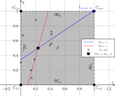
and put the feasible region (see Figure 1)
| (2) |
Note that in this section, for brevity, it is easier to define such that . We also note that is not a set in the traditional sense, but rather a multiset; moreover, we abuse notation slightly by indexing each point and by using superscripts to indicate the Cartesian product of with itself in the context of multisets. We define the sample correlation coefficient of as follows.
Definition 2.1.
The Pearson correlation coefficient (PCC) of a dataset is given by
| (3) |
where and are the sample means of [28].
This definition makes our motivation for imposing constraints on our datasets more obvious. Clearly, if incoming observations were not bounded, worst-case points could be infinitely large, overshadowing the present data and skewing the PCC to an arbitrary degree towards -1 or 1. We also opt for a rectangular feasible region due to its simplicity and similarity to winsorization. For our proofs below, assuming this rectangular region corresponds to the unit square also facilitates our invocation of key theorems in real analysis [33]. We nevertheless consider more complex boundaries below in Section 6.
We also enumerate Student’s t-test for ease of reference below. The monotonic relationship of the p-value with the PCC will also dramatically simplify our analyses.
Theorem 2.2 (Student’s t-test for the Pearson Correlation Coefficient).
The significance of a PCC is given by
| (4) |
where
| (5) |
| (6) |
and is the cumulative density function (CDF) of Student’s t-distribution [6].
Corollary 2.3.
decreases monotonically with .
In online settings, we consider the effect of adding a new point to on the PCC and its p-value, with an interest in the robustness of the PCC to the worst case. We formalize this as follows.
Definition 2.4.
We call
| (7) |
and
| (8) |
the primary sensitivities of within .
For the more general case of adding up to points to , we define the -ary sensitivity, which we will return to briefly in Section 6.
Definition 2.5.
We call
| (9) |
and
| (10) |
the -ary sensitivities of within .
Drawing from Welford’s online algorithm for computing variance and covariance, we leverage the following recurrence relations between and subsequent data points [41].
Theorem 2.6 (Welford’s recurrence relations).
Fix a dataset and new point . Let and be the biased sample standard deviations and sample means, respectively, of . Further, let and be the sample mean of . Then
| (11) |
| (12) |
and
| (13) |
where denotes sample covariance [41].
We will also find that the best linear unbiased estimators (BLUE) for the regression line for a dataset play a role in proving our key theorems [6]. The BLUE parameters can be related to the statistical moments computed by Welford via the Gauss-Markov Theorem [6].
Theorem 2.7 (Gauss-Markov Theorem).
Fix a dataset . Given a model function
| (14) |
regressing onto , the least-squares line is given by
| (15) |
As is often noted in discussions of Gauss-Markov, we observe the following fact, which we formalize as a proposition for ease of reference in Section 3.
Proposition 2.8.
The sets lying on the BLUE lines intersect at the point .
Likewise, we formally state another trivial property of linear regression.
Proposition 2.9.
if and only if .
As to primary sensitivity itself, the following points will play a critical role.
Definition 2.10.
We refer to the points , , , and , which we denote , , , and , respectively, as corner points.
Definition 2.11.
We refer to the points , , , and , which we denote , , , and , respectively, as intersection points.
3 Primary sensitivity
In the following section, we leverage Welford [6] to derive a closed-form function mapping from new points to the quantity . By studying the solutions to this function, we will then be able to trivially compute and .
Substituting Welford’s identities into Definition 2.1, simplifying, and then rewriting the correlation as a function , we have
| (16) |
For brevity, we let , , , , , then observe that we have the following derivatives of :
| (17) |
Proposition 3.1.
For all , if and only if .
Proof.
It suffices to prove our proposition for . If , we must have
| (18) |
meaning
Therefore, . Our proof of the converse proceeds identically. ∎
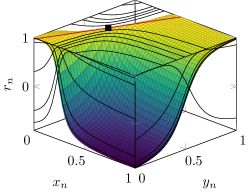
For an illustration of the following, the reader is directed to Figure 2. We note that the comparative complexity of our proof for the first case relative to that for the second is due to the fact that, if the determinant of the Hessian is evaluated for the former, the second-derivative test is inconclusive.
Proposition 3.2.
| (19) |
Proof.
Because is continuous, we observe by the extreme value theorem that it must take maximal and minimal values along the closed and bounded set [33]. It therefore suffices to prove the demonstrandum for . By way of contradiction, we suppose that for all .
By Fermat’s theorem [33], we then know that we must have the first-order condition Furthermore, by Proposition 3.1 and the fact that both and at , we know that must lie on both and . Because both sets are lines, they must intersect at either an infinite set of points or a single point. We then have two cases:
-
(i)
, or
-
(ii)
,
where the second case is due to Proposition 2.8.
Suppose that (i). Then we have for all , in which case, by the fundamental theorem of line integrals [33], must constitute a smooth curve along which the function is constant. However, by the intermediate value theorem [33], we observe that, because is continuous on , it must intersect the boundary at some point . But because is constant on , we must have for all , including for , which contradicts our assumption that all maxima lie in the interior.
We must instead have (ii), in which case . Because it is a local maximum, second-order optimality conditions must obtain [33], i.e., we must have
| (20) |
But by the contrapositive of Proposition 2.9, we know that , meaning that . Then is not a local maximum, which is a contradiction.
Thus, we must have , which completes our proof. ∎
Lemma 3.3.
| (21) |
Proof.
We extend Proposition 3.2 by partitioning into its four edges. Without loss of generality, we consider the edge and extremum and show that . Putting and considering one-dimensional first-order optimality conditions [33], we know that at least one of the following obtain:
-
(i)
, or
-
(ii)
.
If (i), then or . If (ii), then by Proposition 3.1, we must have . This completes our proof. ∎
Likewise, defining the p-value as a function , we obtain similar results.
Proposition 3.4.
If , then there exists a point such that .
Proof.
By Proposition 3.2, we know that . This allows us to invoke the Poincaré-Miranda theorem [33] to infer that there exists a stationary point of in . 111Technically, Poincaré-Miranda supposes that the domain of is the unit square as we do in Figure 2. However, the PCC is invariant to translation and scaling, and so we are in fact able to suppose that without loss of generality. We can then apply Proposition 3.4 to an arbitrary . ∎
Proposition 3.5.
-
(I)
If , then and .
-
(II)
If , then and .
Proof.
It suffices only to prove (I). Due to Corollary 2.3, it also suffices only to show that and . We then simply observe that, because both extrema are positive, we must have , meaning that the extrema do indeed coincide. ∎
Lemma 3.6.
-
(I)
If , then ; otherwise, .
-
(II)
.
Proof.
We have three cases:
-
(i)
,
-
(ii)
, and
-
(iii)
.
Suppose that (i). By Proposition 4.1, we will then have a stationary point. The p-value associated with a PCC of 0 is 1, giving us and therefore (I). By Corollary 2.3, we again know that , meaning that . By Lemma 3.3, we conclude that , giving us (II).
If (ii) or (iii), we apply Proposition 4.2 and Lemma 3.3 to obtain both (I) and (II) and complete our proof. ∎


4 Main algorithm
We are now able to develop our key algorithm, ComputePrimarySensitivities. For its implementation, we assume that , not as we did above. Note that for its implementation below, we write Welford for the online summation of Welford’s parameters and StudentsT to perform the statistical test in Theorem 2.2. We use our earlier recurrence relation for to update merely for brevity; the update rules in Theorem 2.6 could be employed just as appropriately.
Leveraging Lemma 3.3, it computes each intersection point, determines which of them are feasible, and then adds these along with the corner points to to determine which induces the largest changes to the PCC, thereby computing . Afterwards, we test for whether in order to determine whether we have by Lemma 3.6. If so, then either or it is directly derivable from the corner and intersection points, again by Lemma 3.6. If this test fails, then both extrema of lie at the corner and intersection points.
Theorem 4.1.
ComputePrimarySensitivities correctly returns and .
Proof.
This follows trivially from Lemmas 3.3 and 3.6. ∎
Theorem 4.2.
ComputePrimarySensitivities runs in time.
Proof.
Each of lines 3-9, 11-14, 16-17, and 20-21 will require time. The loops and set comprehensions in lines 10, 18, and 19 will run for a constant number of iterations given that the number of corner and intersection points is bounded. Therefore, the algorithm is dominated by the call to Welford in line 2, which will require a single pass to sum all relevant quantities [41]. ∎
Corollary 4.3.
Suppose that the Welford parameters of are computed in advance. Then and can be computed in time.
Proof.
We repeat our proof for Theorem 4.2, albeit excluding Welford in line 2, resulting in a net runtime. ∎
5 Experiments
5.1 Synthetic data
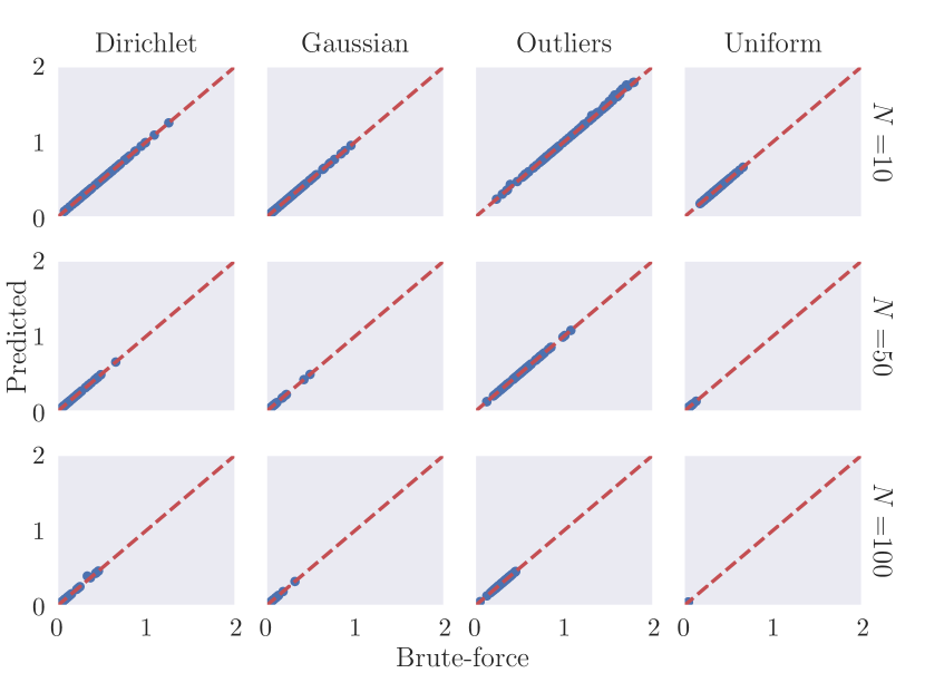
In order to empirically test the correctness of our algorithm, we generated synthetic datasets of varying sizes and compared the results of ComputePrimarySensitivities to brute-force grid search for the four following distributions. First, we sampled each coordinate from an independent uniform distribution on . Second, we drew from centered bivariate Gaussians with covariance matrices given by , where is randomly generated from a uniform distribution at each iteration (multiplication by its own transpose was intended to enforce symmetry and positive definiteness). Third, we sampled from Dirichlet distributions with parameters generated by uniformly sampling . Fourth, we again generated centered bivariate Gaussians, but substituted 10% of each sample with outliers generated from a uniform distribution on [39].
Each sample was generated so as to be of sizes , and for each distribution and , we ran 100 separate experiments. The feasible region was simply set to the bounding box of each dataset, meaning that its size varied dynamically with each experiment. For grid search, we sampled 10 equidistant points along each axis of the feasible region for a total of 100 candidates; larger datasets and finer grids were not employed due to hardware limitations. Likewise, due to the necessity of high numerical precision for computing small changes in p-value, we opted to analyze only for these broad initial tests. All experiments were conducted in Numpy [16] and SciPy [39]. ComputePrimarySensitivities itself was implemented primarily in C for efficiency with a Cython [4] front-end for ease of use.
Results (Figure 3) indicate that ComputePrimarySensitivities consistently predicted values extremely close to that of grid search. For 98.28% of the synthetic datasets, the sensitivities were nearly identical (i.e., within a relative tolerance of ). We conclude that our method correctly predicts the sensitivities of every dataset, with the occasional discrepancies between the two predictions reflecting floating point error or the coarseness of the grid.
5.2 Real-world example: The Great Recession
Among the many use cases for efficiently computing the sensitivity of the PCC, financial markets offer an excellent application for investors weighing portfolio decisions based on relationships between various assets [5, 2, 13]. During the Great Recession of 2008, the financial sector became the epicenter of extreme market volatility [31], prompting investors to closely monitor rapidly evolving market dynamics [1], consider rotating their portfolios to alternative sectors, and otherwise mitigate their exposure to unstable economic conditions [2]. A key factor in portfolio stress-testing was the correlation between broad market indices on one hand and hedge funds, insurance companies, and other financial services on the other. The rationale was that in periods of economic crisis emanating from the financial sector, these services would exhibit far greater instability than the broader markets, suggesting that diverse portfolios would be more likely to mitigate financial risk [31, 1]. However, the correlation between the financial sector and other markets was highly unstable on even a daily basis in 2008 [31], meaning that primary sensitivities of correlations between financial instruments could have been highly informative.
For example, we consider the primary sensitivities of the SPDR S&P 500 ETF Trust (SPY) [36] and Financial Select Sector SPDR Fund (XLF) [35] in September, 2008, when the DOW Jones Industrial Average plummeted to historic lows on the 29th [31]. Computing the PCC between the closing values of SPY and XLF during the week leading up to that date [3, 39], we find that the sample PCC of our dataset is , corresponding to a p-value of (Table 2). While we might be inclined to have very low confidence in a linear relationship between the financial sector and the broader market, we suspect that this could change within a single day. In order to prepare for this possibility, we compute the primary sensitivities of the correlation between SPY and XLF. Although our data do not have a clear feasible region, we set lower bounds of 0 for both instruments and, for their upper bounds, posit that neither will exceed its respective maximum encountered in the foregoing week. Using our framework, we find that the primary sensitivities of are and .
In other words, our analyses indicate that by the end of trading hours on the 30th, it is fully possible that radical changes in market conditions may suddenly nullify the trend of non-linearity between SPY and XLF, rendering the PCC significant and prompting drastic changes in investment strategy. Surely enough, both indices plummet on the 29th, bringing the p-value to a highly significant value of 0.00491 that is well within our predicted primary sensitivity. Additional analysis shows that this p-value is far less sensitive to subsequent fluctuations in price, suggesting that we might be more confident in our investing strategy for at least the remainder of the month.
To confirm the output of our algorithm, we compared the results to that of brute-force search across a much finer grid of 10,000 total points to increase precision for the p-value calculations. We find that our method predicts the correct optima, thereby validating our theory on empirical data. Note also that the sensitivity as per Lemma 3.6; the slight inaccuracy of the brute-force estimate is therefore likely due to the coarseness of the grid.
| Metric | Value | Predicted | Brute-Force |
|---|---|---|---|
| 0.58028 | 1.15630 | 1.15630 | |
| 0.30502 | 0.69498 | 0.69491 |
6 Discussion
Practical applications of our approach are vast, extending to many fields in which dynamic datasets require reliable collinearity measures. In bioinformatics, the strength of associations between genetic markers and phenotypes in genome-wide association studies (GWAS) may be subject to change if data are mined from expanding biobanks [37, 40, 23]. In climatology, associations between temperature and various environmental outcomes like ground water availability are famously subject to reevaluation in light of ongoing studies [18, 38, 26]. In behavioral science and other experimental disciplines, similar analyses may be employed to halt experiments prematurely if the strength of association between variables is determined to be sufficiently robust to new subject data [8, 25, 30]. In the technology sector, dynamic environments like streaming platforms draw from real-time analytics to understand potentially unstable relationships between data streams, user preferences, internet traffic, etc. [27, 21] In differential privacy, the local sensitivity of metrics like the PCC is key for methods like Propose-Test-Release (PTR) [12].
As to the theoretical doors opened by our work, future directions are also numerous. First, in many optimization tasks like linear programming, feasible regions are often presumed to be generally polygonal (or, rather, polyhedral for higher-dimensional tasks) as opposed to simply rectangular [9]. We speculate that similar propositions like those proven above might be straightforwardly adapted for arbitrary piecewise linear boundaries, with basic feasible solutions playing roles similar to corner points in the case of a rectangular domain.
We conjecture that -ary sensitivity can be efficiently computed as well by extending our theory further. In analyses not explicated in this paper, we were able to prove that the worst-case sequence of points to add to a bounded dataset must conform to certain structures, e.g., that each point in the sequence must also be a corner or intersection point. These patterns may offer an opportunity to compute the worst-case sequence via a combinatorial optimization approach.
Finally, our method of leveraging Welford’s identities may be extended to other linear metrics such as covariance and the parameters of the best linear unbiased estimators (BLUE) for simple linear regression [6]. For higher-dimensional datasets, similar analyses might be even extended to covariance matrices or principal components [6].
7 Conclusion
In this work, we develop a rigorous theoretical framework for analyzing changes to the Pearson correlation coefficient (PCC) [28] and its p-value induced by the addition of new data points, as well an algorithm for computing these changes in practice. Our key contributions consist of formulating a recurrence relation for the PCC and p-value via identities vital to Welford’s online algorithm [41], deriving closed-form solutions to this relation, and finally demonstrating that these solutions can be straightforwardly computed in linear or even constant time, depending on whether key parameters are precomputed. In addition to formal proofs of correctness, we validate our method on synthetic and real-world data to empirically confirm its efficacy.
Our code is made available at https://github.com/marc-harary/sensitivity for both practical usage and ongoing algorithmic development in this area.
References
- [1] Tobias Adrian and Hyun Song Shin. Liquidity and leverage. Journal of financial intermediation, 19(3):418–437, 2010.
- [2] Andrew Ang and Joseph Chen. Asymmetric correlations of equity portfolios. Journal of financial Economics, 63(3):443–494, 2002.
- [3] Ran Aroussi. yfinance. https://github.com/ranaroussi/yfinance, 2024. Version 0.2.40.
- [4] Stefan Behnel, Robert Bradshaw, Craig Citro, Lisandro Dalcin, Dag Sverre Seljebotn, and Kurt Smith. Cython: The best of both worlds. Computing in Science & Engineering, 13(2):31–39, 2010.
- [5] John Y Campbell and Samuel B Thompson. Predicting excess stock returns out of sample: Can anything beat the historical average? The Review of Financial Studies, 21(4):1509–1531, 2008.
- [6] George Casella and Roger Berger. Statistical inference. CRC Press, 2024.
- [7] R Dennis Cook. Detection of influential observation in linear regression. Technometrics, 42(1):65–68, 2000.
- [8] Linda Crocker and James Algina. Introduction to classical and modern test theory. ERIC, 1986.
- [9] George B Dantzig. Linear programming. Operations research, 50(1):42–47, 2002.
- [10] Wilfrid J Dixon and Kareb K Yuen. Trimming and winsorization: A review. Statistische Hefte, 15(2):157–170, 1974.
- [11] Jurgen Drews. Drug discovery: a historical perspective. science, 287(5460):1960–1964, 2000.
- [12] Cynthia Dwork, Aaron Roth, et al. The algorithmic foundations of differential privacy. Foundations and Trends® in Theoretical Computer Science, 9(3–4):211–407, 2014.
- [13] Eugene F Fama and Kenneth R French. The cross-section of expected stock returns. the Journal of Finance, 47(2):427–465, 1992.
- [14] William H. Greene. Econometric Analysis. Pearson Education, 7th edition, 2003.
- [15] Damodar N Gujarati and Dawn C Porter. Basic econometrics. McGraw-hill, 2009.
- [16] Charles R. Harris, K. Jarrod Millman, Stéfan J. van der Walt, Ralf Gommers, Pauli Virtanen, David Cournapeau, Eric Wieser, Julian Taylor, Sebastian Berg, Nathaniel J. Smith, Robert Kern, Matti Picus, Stephan Hoyer, Marten H. van Kerkwijk, Matthew Brett, Allan Haldane, Jaime Fernández del Río, Mark Wiebe, Pearu Peterson, Pierre Gérard-Marchant, Kevin Sheppard, Tyler Reddy, Warren Weckesser, Hameer Abbasi, Christoph Gohlke, and Travis E. Oliphant. NumPy: A guide to numpy, 2020.
- [17] Fumio Hayashi. Econometrics. Princeton University Press, 2011.
- [18] Isaac M Held and Brian J Soden. Robust responses of the hydrological cycle to global warming. Journal of climate, 19(21):5686–5699, 2006.
- [19] Peter J Huber. Robust statistics, volume 523. John Wiley & Sons, 2004.
- [20] James P Hughes, Stephen Rees, S Barrett Kalindjian, and Karen L Philpott. Principles of early drug discovery. British journal of pharmacology, 162(6):1239–1249, 2011.
- [21] Folasade Olubusola Isinkaye, Yetunde O Folajimi, and Bolande Adefowoke Ojokoh. Recommendation systems: Principles, methods and evaluation. Egyptian informatics journal, 16(3):261–273, 2015.
- [22] Jonathan M Karpoff. The relation between price changes and trading volume: A survey. Journal of Financial and quantitative Analysis, 22(1):109–126, 1987.
- [23] Thomas J Littlejohns, Jo Holliday, Lorna M Gibson, Steve Garratt, Niels Oesingmann, Fidel Alfaro-Almagro, Jimmy D Bell, Chris Boultwood, Rory Collins, Megan C Conroy, et al. The uk biobank imaging enhancement of 100,000 participants: rationale, data collection, management and future directions. Nature communications, 11(1):2624, 2020.
- [24] Ricardo A Maronna, R Douglas Martin, Victor J Yohai, and Matías Salibián-Barrera. Robust statistics: theory and methods (with R). John Wiley & Sons, 2019.
- [25] Douglas C Montgomery. Design and analysis of experiments. John wiley & sons, 2017.
- [26] Colin P Morice, John J Kennedy, Nick A Rayner, and Phil D Jones. Quantifying uncertainties in global and regional temperature change using an ensemble of observational estimates: The hadcrut4 data set. Journal of Geophysical Research: Atmospheres, 117(D8), 2012.
- [27] Thuy TT Nguyen and Grenville Armitage. A survey of techniques for internet traffic classification using machine learning. IEEE communications surveys & tutorials, 10(4):56–76, 2008.
- [28] Karl Pearson. Vii. note on regression and inheritance in the case of two parents. proceedings of the royal society of London, 58(347-352):240–242, 1895.
- [29] Ioannis Pitas and Anastasios N Venetsanopoulos. Order statistics in digital image processing. Proceedings of the IEEE, 80(12):1893–1921, 1992.
- [30] Tenko Raykov and George A Marcoulides. Introduction to psychometric theory. Routledge, 2011.
- [31] Carmen M Reinhart and Kenneth S Rogoff. The aftermath of financial crises. American Economic Review, 99(2):466–472, 2009.
- [32] Peter J Rousseeuw and Annick M Leroy. Robust regression and outlier detection. John wiley & sons, 2005.
- [33] Walter Rudin et al. Principles of mathematical analysis, volume 3. McGraw-hill New York, 1964.
- [34] Gregory Sliwoski, Sandeepkumar Kothiwale, Jens Meiler, and Edward W Lowe. Computational methods in drug discovery. Pharmacological reviews, 66(1):334–395, 2014.
- [35] State Street Global Advisors. Financial select sector spdr fund. Prospectus, 2008. Retrieved from SSGA website.
- [36] State Street Global Advisors. Spdr s&p 500 etf trust. Prospectus, 2008. Retrieved from SSGA website.
- [37] Vivian Tam, Nikunj Patel, Michelle Turcotte, Yohan Bossé, Guillaume Paré, and David Meyre. Benefits and limitations of genome-wide association studies. Nature Reviews Genetics, 20(8):467–484, 2019.
- [38] Richard G Taylor, Bridget Scanlon, Petra Döll, Matt Rodell, Rens Van Beek, Yoshihide Wada, Laurent Longuevergne, Marc Leblanc, James S Famiglietti, Mike Edmunds, et al. Ground water and climate change. Nature climate change, 3(4):322–329, 2013.
- [39] Pauli Virtanen, Ralf Gommers, Travis E Oliphant, Matt Haberland, Tyler Reddy, David Cournapeau, Evgeni Burovski, Pearu Peterson, Warren Weckesser, Jonathan Bright, et al. Scipy 1.0: fundamental algorithms for scientific computing in python. Nature methods, 17(3):261–272, 2020.
- [40] William YS Wang, Bryan J Barratt, David G Clayton, and John A Todd. Genome-wide association studies: theoretical and practical concerns. Nature Reviews Genetics, 6(2):109–118, 2005.
- [41] BP Welford. Note on a method for calculating corrected sums of squares and products. Technometrics, 4(3):419–420, 1962.