Recursive PAC-Bayes: A Frequentist Approach to Sequential Prior Updates
Recursive PAC-Bayes: A Frequentist Approach to Sequential Prior Updates with No Information Loss
Abstract
PAC-Bayesian analysis is a frequentist framework for incorporating prior knowledge into learning. It was inspired by Bayesian learning, which allows sequential data processing and naturally turns posteriors from one processing step into priors for the next. However, despite two and a half decades of research, the ability to update priors sequentially without losing confidence information along the way remained elusive for PAC-Bayes. While PAC-Bayes allows construction of data-informed priors, the final confidence intervals depend only on the number of points that were not used for the construction of the prior, whereas confidence information in the prior, which is related to the number of points used to construct the prior, is lost. This limits the possibility and benefit of sequential prior updates, because the final bounds depend only on the size of the final batch.
We present a novel and, in retrospect, surprisingly simple and powerful PAC-Bayesian procedure that allows sequential prior updates with no information loss. The procedure is based on a novel decomposition of the expected loss of randomized classifiers. The decomposition rewrites the loss of the posterior as an excess loss relative to a downscaled loss of the prior plus the downscaled loss of the prior, which is bounded recursively. As a side result, we also present a generalization of the split-kl and PAC-Bayes-split-kl inequalities to discrete random variables, which we use for bounding the excess losses, and which can be of independent interest. In empirical evaluation the new procedure significantly outperforms state-of-the-art.
1 Introduction
PAC-Bayesian analysis was born from an attempt to derive frequentist generalization guarantees for Bayesian-style prediction rules (Shawe-Taylor and Williamson, 1997, McAllester, 1998). The motivation was to provide a way to incorporate prior knowledge into the frequentist analysis of generalization. PAC-Bayesian bounds provide high-probability generalization guarantees for randomized classifiers. A randomized classifier is defined by a distribution on a set of prediction rules , which is used to sample a prediction rule each time a prediction is to be made. Bayesian posterior is an example of a randomized classifier, whereas PAC-Bayesian bounds hold generally for all randomized classifiers. Prior knowledge is encoded through a prior distribution on , and the complexity of a posterior distribution is measured by the Kullback-Leibler (KL) divergence from the prior, . PAC-Bayesian generalization guarantees are optimized by posterior distributions that optimize a trade-off between empirical data fit and divergence from the prior in the KL sense.
Selection of a “good” prior plays an important role in the PAC-Bayesian bounds. If one manages to foresee which prediction rules are likely to produce low prediction error and allocate a higher prior mass for them, then the bounds are tighter, because the posterior only needs to make a small deviation from the prior. But if the prior mass on well-performing prediction rules is small, the bounds are loose. A major technique to design good priors is to use part of the data to estimate a good prior and the rest of the data to compute a PAC-Bayes bound. It is known as data-dependent or data-informed priors (Ambroladze et al., 2007). However, all existing approaches to data-informed priors have three major disadvantages. The first is that the bounds are computed on “the rest of the data” that were not used in construction of the prior. Thus, the sample size in the bounds is only a fraction of the total sample size. Therefore, empirically data-informed priors are not always helpful. In many cases starting with an uninformed prior and using all the data to compute the posterior and the bound turns to be superior to sacrificing part of the data for prior construction (Ambroladze et al., 2007, Mhammedi et al., 2019). The second disadvantage is that all the confidence information about the prior is lost in the process. In particular, a prior trained on a few data points is treated in the same way as a prior trained on a lot of data. And a third related disadvantage is that sequential data processing is detrimental, because the bounds only depend on the size of the last chunk and all the confidence information from processing earlier chunks is lost in the process.
Our main contribution is a new (and simple) way of decomposing the loss of a randomized classifier defined by the posterior. We write it as an excess loss relative to a downscaled loss of the randomized classifier defined by the prior plus the downscaled loss of the randomized classifier defined by the prior. The excess loss can be bounded using PAC-Bayes-Empirical-Bernstein-style inequalities (Tolstikhin and Seldin, 2013, Mhammedi et al., 2019, Wu et al., 2021, Wu and Seldin, 2022), whereas the loss of the randomized classifier defined by the prior can be bounded recursively. The recursive bound can both use the data used for construction of the prior and “the rest of the data”, and thereby preserves confidence information on the prior. Our contribution stands out relative to all prior work on PAC-Bayes, and in fact all prior work on frequentist generalization bounds, because it makes sequential data processing and sequential prior updates meaningful and beneficial.
We note that while several recent papers experimented with sequential posterior updates by using martingale-style analysis, in all these works the prior remained fixed and only the posterior was changing (Chugg et al., 2023, Biggs and Guedj, 2023, Rodríguez-Gálvez et al., 2024). Another line of work used tools from online learning to derive PAC-Bayesian bounds (Jang et al., 2023), and in this context Haddouche and Guedj (2023) have used sequential prior updates, but their bounds hold for a uniform aggregation of sequentially constructed posteriors, which is different from standard posteriors studied in our work. The confidence bounds in their work come primarily from aggregation rather than confidence in individual posteriors in the sequence. Our work is the first one allowing sequential prior updates without loss of confidence information.
An additional side contribution of independent interest is a generalization of the split-kl and PAC-Bayes-split-kl inequalities of Wu and Seldin (2022) from ternary to general discrete random variables. It is based on a novel representation of discrete random variables as a superposition of Bernoulli random variables.
The paper is organized in the following way. In Section 2 we briefly survey the evolution of data-informed priors in PAC-Bayes and present our main idea behind Recursive PAC-Bayes; in Section 3 we present our generalization of the split-kl and PAC-Bayes-split-kl inequalities, which are later used to bound the excess losses; in Section 4 we present the Recursive PAC-Bayes bound; in Section 5 we present an empirical evaluation; and in Section 6 we conclude with a discussion.
2 The evolution of data-informed priors and the idea of Recursive PAC-Bayes
In this section we briefly survey the evolution of data-informed priors, and then present our construction of Recursive PAC-Bayes. We consider the standard binary classification setting, with being a sample space, a label space, a set of prediction rules , and the zero-one loss function, where denotes the indicator function. We let denote a distribution on and an i.i.d. sample from . Let be the expected and the empirical loss.
Let be a distribution on . A randomized classifier associated with samples a prediction rule according to for each sample , and applies it to make a prediction . The expected loss of such randomized classifier, which we call , is and the empirical loss is . For brevity we use to denote .
We use to denote the Kullback-Leibler divergence between two probability distributions, and (Cover and Thomas, 2006). For we further use to denote the Kullback-Leibler divergence between two Bernoulli distributions with biases and .
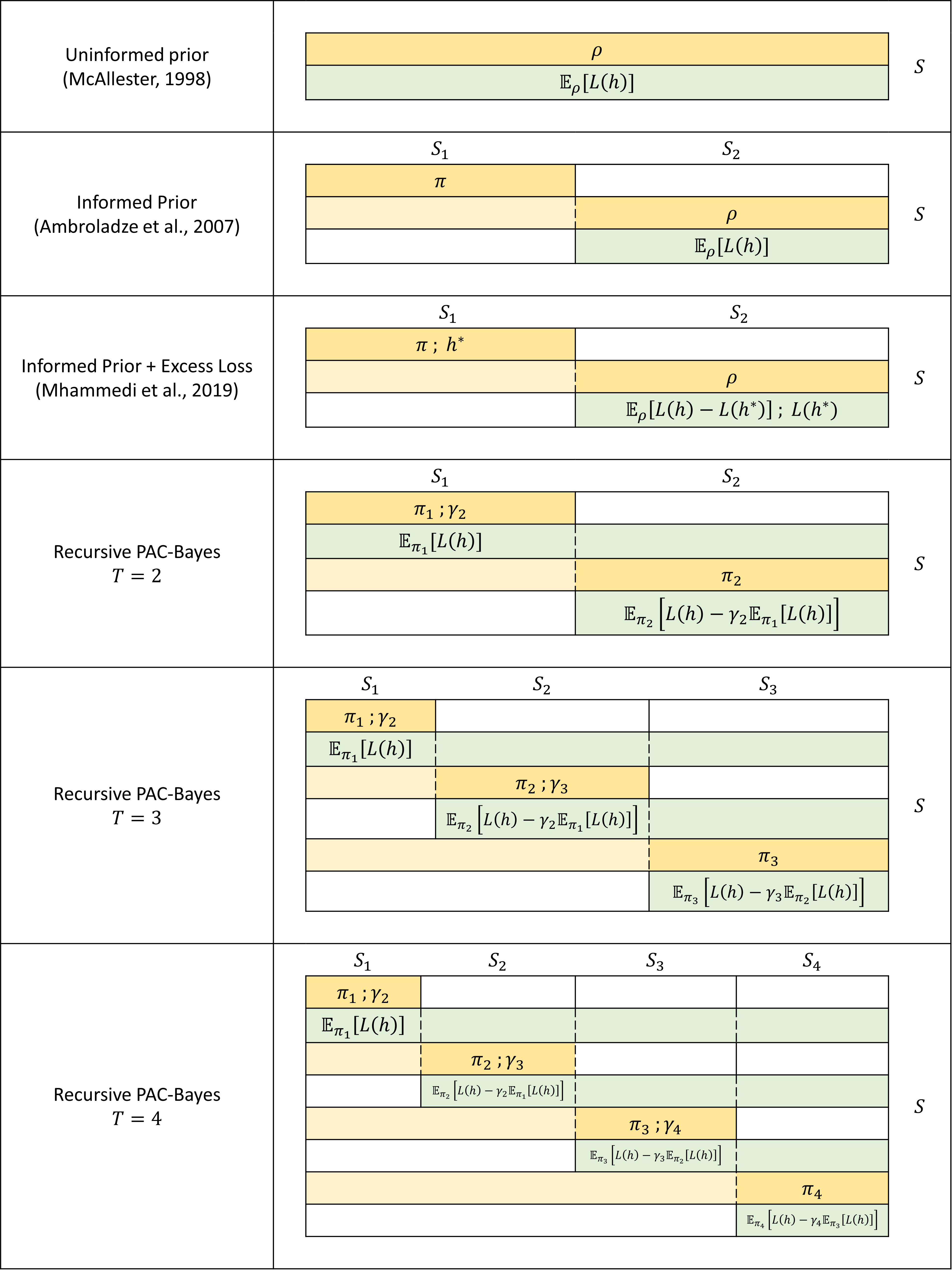
The goal of PAC-Bayes is to bound . Below we present how the bounds on have evolved. In Appendix A we also provide a graphical illustration of the evolution.
Uninformed priors
Early work on PAC-Bayes used uninformed priors (McAllester, 1998). An uniformed prior is a distribution on that is independent of the data . A classical, and still one of the tightest bounds, is the following.
Theorem 1 (PAC-Bayes- Inequality, Seeger, 2002, Maurer, 2004).
For any probability distribution on that is independent of and any :
where is the set of all probability distributions on , including those dependent on .
A posterior that minimizes has to balance between allocating higher mass to prediction rules with small and staying close to in the sense. Since has to be independent of , typical uninformed priors aim “to leave maximal options open” for by staying close to uniform.
Data-informed priors
Ambroladze et al. (2007) proposed to split the data into two disjoint sets, , and use to construct a data-informed prior and compute a bound on using and . Since in this approach is independent of , Theorem 1 can be applied. The advantage is that can use to give higher mass to promising classifiers, thus relaxing the regularization pressure and making it easier for to allocate even higher mass to well-performing classifiers (those with small ). The disadvantage is that the sample size in the bound (the in the denominator) decreases from the size of to the size of . Indeed, Ambroladze et al. observed that the sacrifice of for prior construction does not always pay off.
Data-informed priors + excess loss
Mhammedi et al. (2019) observed that if we have already sacrificed for the construction of , we could also use it to construct a reference prediction rule , typically an Empirical Risk Minimizer (ERM) on . They then employed the decomposition
and used to give a PAC-Bayesian bound on and a single-hypothesis bound on . The quantity is known as excess loss. The advantage of this approach is that when is a good approximation of , the excess loss has lower variance than the plain loss and, therefore, is more efficient to bound, whereas the single-hypothesis bound on does not involve the term. Therefore, it is generally beneficial to use excess losses in combination with data-informed priors. However, as with the previous approach, sacrificing to learn and means that the denominator in the bounds ( in Theorem 1) reduces to the size of , and it does not always pay off. (We note that the excess loss is not binary and not in the interval, and in order to exploit small variance it is actually necessary to apply a PAC-Bayes-Empirical-Bernstein-style inequality (Tolstikhin and Seldin, 2013, Mhammedi et al., 2019, Wu et al., 2021) or the PAC-Bayes-split-kl inequality (Wu and Seldin, 2022) rather than Theorem 1, but the point about reduced sample size still applies.)
Recursive PAC-Bayes (new)
We introduce the following decomposition of the loss
| (1) |
As before, we decompose into two disjoint sets . We make the following major observations:
-
•
The quantity on the right is “of the same kind” as on the left.
-
•
We can take an uninformed prior and apply Theorem 1 (or any other suitable PAC-Bayes bound) to bound . (The term in the bound on will be .)
-
•
We can restrict to depend only on , but still use all the data in calculation of the PAC-Bayes bound on , because is a posterior relative to , and a posterior is allowed to depend on all the data, and in particular on any subset of the data. Therefore, the empirical loss can be computed on all the data , and the denominator of the bound in Theorem 1 can be the size of , and not the size of . This is what we call preservation of confidence information on , because all the data are used to construct a confidence bound on , and not just . This is in contrast to the bound on in the approach of Mhammedi et al. (2019), which only allows to use for bounding . Note that while we use all the data in calculation of the bound, we only use and in the construction of . Nevertheless, we can still use the knowledge that we will have samples when we reach the estimation phase, i.e., when constructing we can leave the denominator of the bound at , allowing more aggressive deviation from .
-
•
If we restrict to depend only on , then it is a valid prior for estimation of any posterior quantity based on . Thus, if we also restrict to depend only on , we can use any PAC-Bayes-Empirical-Bernstein-style inequality or the PAC-Bayes-split-kl inequality to estimate the excess loss based on , i.e., based on . If is a good approximation of and is not close to zero, then the excess loss is more efficient to bound than the plain loss .
-
•
In general, since is expected to improve on , it is natural to set . However, is not allowed to depend on , because otherwise becomes a biased estimate of . We discuss the choice of in more detail when we present the bound and the experiments.
-
•
Biggs and Guedj (2023) have proposed a sequential martingale-style evaluation of a martingale version of and in the approach of Mhammedi et al., but it has not been shown to yield significant improvements yet. The same “martingalization” can be directly applied to our decomposition, but to keep things simple we stay with the basic decomposition.
-
•
Finally, we note that we can split further and apply (1) recursively to bound .
To set notation for recursive decomposition, we use to denote a sequence of distributions on , where is an uninformed prior and is the final posterior. We use to denote a sequence of coefficients. For we then have the recursive decomposition
| (2) |
To construct we split the data into non-overlapping subsets, . We restrict to depend on only, and we use to estimate (recursively) (see Figure 1 in Appendix A). Note that is used both for construction of and for estimation of (it is both in and ), resulting in efficient use of the data. It is possible to use any standard PAC-Bayes bound, e.g., Theorem 1, to bound , and any PAC-Bayes-Empirical-Bernstein-style bound or the PAC-Bayes-split-kl bound to bound the excess losses . The excess losses take more than three values, so in the next section we present a generalization of the PAC-Bayes-split-kl inequality to general discrete random variables, which may be of independent interest. The Recursive PAC-Bayes bound is presented in Section 4.
3 Split-kl and PAC-Bayes-split-kl inequalities for discrete random variables
The inequality is one of the tightest concentration of measure inequalities for binary random variables. Letting denote the upper inverse of and the lower inverse, it states the following.
Theorem 2 ( Inequality (Langford, 2005, Foong et al., 2021, 2022)).
Let be independent random variables bounded in the interval and with for all . Let be the empirical mean. Then, for any :
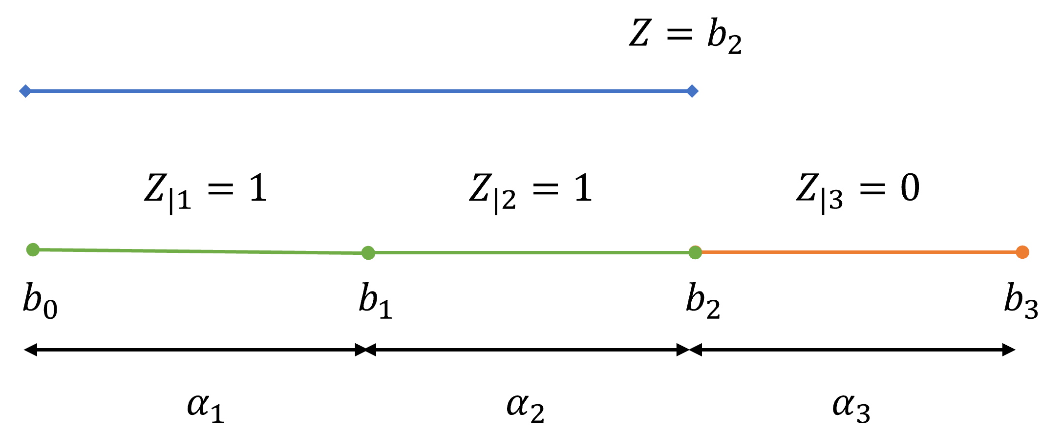
While the inequality is tight for binary random variables, it is loose for random variables taking more than two values due to its inability to exploit small variance. To address this shortcoming Wu and Seldin (2022) have presented the split-kl and PAC-Bayes-split-kl inequalities for ternary random variables. Ternary random variables naturally appear in a variety of applications, including analysis of excess losses, certain ways of analysing majority votes, and in learning with abstention. The bound of Wu and Seldin is based on decomposition of a ternary random variable into a pair of binary random variables and application of the inequality to each of them. Their decomposition yields a tight bound in the binary and ternary case, but loose otherwise. The same decomposition was used by Biggs and Guedj (2023) to derive a slight variation of the inequality, with the same limitations. We present a novel decomposition of discrete random variables into a superposition of binary random variables. Unlike the decomposition of Wu and Seldin, which only applies in the ternary case, our decomposition applies to general discrete random variables. By combining it with bounds for the binary elements we obtain a tight bound. The decomposition is presented formally below and illustrated graphically in Figure 2 in Appendix A.
3.1 Split-kl inequality
Let be a -valued random variable with . For define and . Then . For a sequence of -valued random variables with the same support, let denote the elements of binary decomposition of .
Theorem 3 (Split- inequality for discrete random variables).
Let be i.i.d. random variables taking values in with for all . Let . Then for any :
Proof.
Let , then and
where the first inequality is by the decomposition of and the second inequality is by the union bound and Theorem 2. ∎
3.2 PAC-Bayes-Split-kl inequality
Let be a -valued loss function. (To connect it to the earlier examples, in the binary prediction case we would have with elements and , but we will need a more general space later.) For let . Let be an unknown distribution on . For let and . Let be an i.i.d. sample according to and .
Theorem 4 (PAC-Bayes-Split-kl Inequality).
For any distribution on that is independent of and any :
where is the set of all possible probability distributions on that can depend on .
Proof.
We have and . Therefore,
where the first inequality is by the decomposition of and the second inequality is by the union bound and application of Theorem 1 to (note that is a zero-one loss function). ∎
4 Recursive PAC-Bayes bound
Now we derive a Recursive PAC-Bayes bound based on the loss decomposition in equation (2). In order to bound we need empirical estimates of . We denote , where is a product distribution on and is sampled according to . We define , then . We let and . We let , then .
For each sample we sample a prediction rule to serve for . We let to be the resulting sequence of prediction rules sampled independently according to . We only use the first elements of the sequence in accordance with the size of the sample used in the corresponding estimation. We define , where and we take the first elements from , one for each sample. Note that . Now we are ready to state the bound.
Theorem 5 (Recursive PAC-Bayes Bound).
Let be an i.i.d. sample split in an arbitrary way into non-overlapping subsamples, and let and . Let . Let be a sequence of distributions on , where is allowed to depend on , but not the rest of the data. Let be a sequence of coefficients, where is allowed to depend on , but not the rest of the data. For let be a set of distributions on , which are allowed to depend on . Then for any :
where is a PAC-Bayes bound on defined recursively as follows. For
For we let denote a PAC-Bayes bound on given by
and then
| (3) |
Proof.
Discussion
-
•
Note that can be constructed sequentially, but can only be constructed based on the data in , meaning that in the construction of we can only rely on , but not on . Also note that is part of both and (see Figure 1 in Appendix A for a graphical illustration). In other words, when we evaluate the bounds we can use additional data. And even though the additional data can only be used in the evaluation stage, we can still use the knowledge that we will get more data for evaluation when we construct . For example, we can take
(4) The empirical losses above are calculated on corresponding to , but the sample sizes correspond to the size of the validation set rather than the size of . This allows to be more aggressive in deviating with from by sustaining larger terms.
-
•
Similarly, can also be constructed sequentially, as long as only depends on (otherwise becomes a biased estimate of ).
-
•
We naturally want to have improvement over recursion rounds, meaning . Plugging this into (3), we obtain , which implies that we want to be sufficiently small to satisfy . At the same time, should be non-negative. Therefore, improvement over recursion steps can only be maintained as long as . We also note that if , then overly small can increase the excess loss. Thus, unless the loss is close to zero, should not be too small either.
5 Experiments
In this section, we provide an empirical comparison of our Recursive PAC-Bayes (RPB) procedure to the following prior work: i) Uninformed priors (Uninformed), (Dziugaite and Roy, 2017); ii) Data-informed priors (Informed) (Ambroladze et al., 2007, Pérez-Ortiz et al., 2021); iii) Data-informed prior + excess loss (Informed + Excess) (Mhammedi et al., 2019, Wu and Seldin, 2022). All the experiments were run on a laptop.
We start with describing the details of the optimization procedure, and then present the results.
5.1 Details of the optimization and evaluation procedure
We constructed sequentially using the optimization objective (4), and computed the bound using the recursive procedure in Theorem 5. There are a few technical details concerning convexity of the optimization procedure and infinite size of the set of prediction rules that we address next.
5.1.1 Convexification of the loss functions
The functions defined in Section 4 are non-convex and non-differentiable: . In order to facilitate optimization, we approximate the external indicator function by a sigmoid function with a fixed parameter specified in Section B.3.
Furthermore, since the zero-one loss is also non-differentiable, we adopt the cross-entropy loss, as in most modern training procedures (Pérez-Ortiz et al., 2021). Specifically, for a -class classification problem, let represent the function implemented by the neural network, assigning each class a real value. Let be the assignment, with being the -th value of the vector. To convert this real-valued vector into a probability distribution over classes, we apply the softmax function , where for some for each entry. The cross-entropy loss is defined by . However, since this loss is unbounded, whereas the PAC-Bayes-kl bound requires losses within , we enforce a -valued cross-entropy loss by first lower-bounding the probability assigned to by taking for , and then rescaling it to by taking (Dziugaite and Roy, 2017).
We emphasize that in the evaluation of the bound (using Theorem 5), we directly compute the zero-one loss and the functions without employing the approximations.
5.1.2 Relaxation of the PAC-Bayes-kl bound
The PAC-Bayes- bound is often criticized for being unfriendly to optimization (Rodríguez-Gálvez et al., 2024). Therefore, several relaxations have been proposed, including the PAC-Bayes-classic bound (McAllester, 1999), the PAC-Bayes- bound (Thiemann et al., 2017), and the PAC-Bayes-quadratic bound (Rivasplata et al., 2019, Pérez-Ortiz et al., 2021), among others. In our optimization we have adopted the bound of McAllester (1999) instead of the kl-based bounds in Equation (4).
We again emphasize that in the evaluation of the bound we used the kl-based bounds in Theorem 5.
5.1.3 Estimation of
Due to the infinite size of and lack of a closed-form expression for and appearing in Theorem 5, we approximate them by sampling (Pérez-Ortiz et al., 2021). For optimization, we sample one classifier for each mini-batch during stochastic gradient descent. For evaluation, we sample one classifier for each data in the corresponding evaluation dataset. Due to approximation of the empirical quantities the final bound in Theorem 5 requires an additional concentration bound. (We note that the extra bound is only required for computation of the final bound, but not for optimization of .) Specifically, let be samples drawn i.i.d. from . Then for any function taking values in (which is the case for and ) and we have
It is worth noting that is evaluated for a fixed , meaning that there is no selection involved, and therefore no term appears in the bound above. We, of course, take a union bound over all the quantities being estimated.
5.2 Experimental results
We evaluated our approach and compared it to prior work using multi-class classification tasks on MNIST (LeCun and Cortes, 2010) and Fashion MNIST (Xiao et al., 2017) datasets, both with 60000 training data. The experimental setup was based on the work of Dziugaite and Roy (2017) and Pérez-Ortiz et al. (2021). Similar to them we used Gaussian distributions for all the priors and posteriors, modeled by probabilistic neural networks. Technical details are provided in B.
| MNIST | Fashion MNIST | |||||
|---|---|---|---|---|---|---|
| Train 0-1 | Test 0-1 | Bound | Train 0-1 | Test 0-1 | Bound | |
| Uninf. | .318 (1e-3) | .310 (3e-3) | .441 (1e-3) | .369 (4e-3) | .372 (5e-3) | .462 (4e-3) |
| Inf. | .338 (2e-3) | .332 (5e-3) | .379 (3e-3) | .381 (2e-3) | .385 (6e-3) | .414 (3e-3) |
| Inf. + Ex. | .189 (3e-3) | .182 (4e-3) | .356 (5e-3) | .281 (4e-3) | .287 (3e-3) | .428 (5e-3) |
| RPB | .123 (5e-3) | .141 (6e-3) | .331 (.011) | .232 (4e-3) | .220 (8e-3) | .359 (4e-3) |
| RPB | .104 (5e-3) | .104 (5e-3) | .215 (4e-3) | .181 (6e-3) | .193 (7e-3) | .279 (6e-3) |
| RPB | .098 (7e-3) | .096 (5e-3) | .187 (6e-3) | .171 (.012) | .177 (0.01) | .264 (6e-3) |
| Test 0-1 | ||||||
|---|---|---|---|---|---|---|
| 1 | 60000 | .084 (2e-3) | .432 (9e-3) | .195 (.016) | ||
| 2 | 58125 | .029 (5e-3) | .020 (6e-4) | .134 (5e-3) | .351 (7e-3) | .143 (8e-e) |
| 3 | 56250 | .050 (5e-3) | .006 (3e-4) | .102 (4e-3) | .277 (3e-3) | .115 (6e-3) |
| 4 | 52500 | .051 (3e-3) | .003 (2e-4) | .090 (4e-3) | .228 (4e-3) | .108 (7e-3) |
| 5 | 45000 | .050 (3e-3) | .003 (3e-4) | .085 (4e-3) | .199 (4e-3) | .104 (.011) |
| 6 | 30000 | .053 (5e-3) | .002 (2e-4) | .088 (6e-3) | .187 (6e-3) | .096 (5e-3) |
The empirical evaluation is presented in Table 1. For the Uninformed approach, we trained and evaluated the bound using the entire training dataset directly. For the other two baseline methods, Informed and Informed + Excess Loss, we used half of the training data to train the informed prior and an ERM for the excess loss, and the other half to learn the posterior. For our Recursive PAC-Bayes (RPB), we chose for all , and conducted experiments with , , and to study the impact of recursion depth. (Each value of corresponded to a separate run of the algorithm and a separate evaluation of the bound, i.e., they should not be seen as successive refinements.) We applied geometric split of the data, where at each recursion step the data were split in two equal halves. Specifically, for the split was (30000,30000) points, for it was (7500, 7500, 15000, 30000) points, and for it was (1875, 1875, 3750, 7500, 15000, 30000) points. The motivation was to let early recursion steps with few data points efficiently learn the prior, while keeping enough data for fine-tuning in the later steps. Note that with this approach the value of , which is in the denominator of the bounds in Theorem 5, is at least .
| Test 0-1 | ||||||
|---|---|---|---|---|---|---|
| 1 | 60000 | .052 (1e-3) | .459 (.014) | .323 (.011) | ||
| 2 | 58125 | .064 (8e-3) | .011 (1e-3) | .149 (.010) | .378 (7e-3) | .226 (.012) |
| 3 | 56250 | .088 (3e-3) | .003 (4e-4) | .133 (3e-3) | .322 (3e-3) | .206 (.011) |
| 4 | 52500 | .094 (8e-3) | .002 (3e-4) | .131 (9e-3) | .292 (9e-3) | .226 (9e-3) |
| 5 | 45000 | .088 (5e-3) | .001 (1e-4) | .120 (5e-3) | .266 (6e-3) | .192 (6e-3) |
| 6 | 30000 | .093 (6e-3) | .002 (1e-4) | .131 (7e-3) | .264 (6e-3) | .177 (0.01) |
Table 1 shows that , which corresponds to the data split in the Informed and the Informed + Excess Loss approaches, already outperforms prior work, whereas deeper recursion yields dramatic improvements.
Tables 2 and 3 provide a glimpse into the training progress of RPB with by showing the evolution of the key quantities along the recursive process. Similar tables for other values of are provided in Section B.4, along with training details for other methods. The tables show an impressive reduction of the term and significant improvement of the bound as the recursion proceeds, demonstrating effectiveness of the approach.
6 Discussion
We have presented the first PAC-Bayesian bound that supports sequential prior updates and preserves confidence information on the prior. The work closes a long-standing gap between Bayesian and Frequentist learning by making sequential data processing and sequential updates of prior knowledge meaningful and beneficial in the frequentist framework, as it has always been in the Bayesian framework. We have shown that apart from theoretical beauty the approach is beneficial in practice.
Acknowledgments and Disclosure of Funding
YW acknowledges support from the Novo Nordisk Foundation, grant number NNF21OC0070621. YZ acknowledge Ph.D. funding from Novo Nordisk A/S. BECA acknowledges funding from the ANR grant project BACKUP ANR-23-CE40-0018-01.
References
- Ambroladze et al. (2007) Amiran Ambroladze, Emilio Parrado-Hernández, and John Shawe-Taylor. Tighter PAC-Bayes bounds. In Advances in Neural Information Processing Systems (NeurIPS), 2007.
- Biggs and Guedj (2023) Felix Biggs and Benjamin Guedj. Tighter PAC-Bayes generalisation bounds by leveraging example difficulty. In Proceedings on the International Conference on Artificial Intelligence and Statistics (AISTATS), 2023.
- Chugg et al. (2023) Ben Chugg, Hongjian Wang, and Aaditya Ramdas. A unified recipe for deriving (time-uniform) PAC-Bayes bounds. Journal of Machine Learning Research, 24(372), 2023.
- Cover and Thomas (2006) Thomas M. Cover and Joy A. Thomas. Elements of Information Theory. Wiley Series in Telecommunications and Signal Processing, 2nd edition, 2006.
- Dziugaite and Roy (2017) Gintare Karolina Dziugaite and Daniel M. Roy. Computing nonvacuous generalization bounds for deep (stochastic) neural networks with many more parameters than training data. In Proceedings of the Conference on Uncertainty in Artificial Intelligence (UAI), 2017.
- Foong et al. (2021) Andrew Foong, Wessel Bruinsma, David Burt, and Richard Turner. How tight can pac-bayes be in the small data regime? In Advances in Neural Information Processing Systems (NeurIPS), 2021.
- Foong et al. (2022) Andrew Y. K. Foong, Wessel P. Bruinsma, and David R. Burt. A note on the chernoff bound for random variables in the unit interval. arXiv preprint arXiv.2205.07880, 2022.
- Haddouche and Guedj (2023) Maxime Haddouche and Benjamin Guedj. PAC-Bayes generalisation bounds for heavy-tailed losses through supermartingales. Transactions on Machine Learning Research Journal, 2023.
- Jang et al. (2023) Kyoungseok Jang, Kwang-Sung Jun, Ilja Kuzborskij, and Francesco Orabona. Tighter PAC-Bayes bounds through coin-betting. In Proceedings of the Conference on Learning Theory (COLT), 2023.
- Langford (2005) John Langford. Tutorial on practical prediction theory for classification. Journal of Machine Learning Research, 6, 2005.
- LeCun and Cortes (2010) Yann LeCun and Corinna Cortes. MNIST handwritten digit database. 2010. URL http://yann.lecun.com/exdb/mnist/.
- Maurer (2004) Andreas Maurer. A note on the PAC-Bayesian theorem. arXiv preprint cs/0411099, 2004.
- McAllester (1998) David McAllester. Some PAC-Bayesian theorems. In Proceedings of the Conference on Learning Theory (COLT), 1998.
- McAllester (1999) David McAllester. Some PAC-Bayesian theorems. Machine Learning, 37, 1999.
- Mhammedi et al. (2019) Zakaria Mhammedi, Peter Grünwald, and Benjamin Guedj. PAC-Bayes un-expected Bernstein inequality. In Advances in Neural Information Processing Systems (NeurIPS), 2019.
- Pérez-Ortiz et al. (2021) María Pérez-Ortiz, Omar Rivasplata, John Shawe-Taylor, and Csaba Szepesvári. Tighter risk certificates for neural networks. Journal of Machine Learning Research, 2021.
- Rivasplata et al. (2019) Omar Rivasplata, Vikram M Tankasali, and Csaba Szepesvari. Pac-bayes with backprop. arXiv preprint arXiv:1908.07380, 2019.
- Rodríguez-Gálvez et al. (2024) Borja Rodríguez-Gálvez, Ragnar Thobaben, and Mikael Skoglund. More PAC-Bayes bounds: From bounded losses, to losses with general tail behaviors, to anytime validity. Journal of Machine Learning Research, 25(110), 2024.
- Seeger (2002) Matthias Seeger. PAC-Bayesian generalization error bounds for Gaussian process classification. Journal of Machine Learning Research, 3, 2002.
- Shawe-Taylor and Williamson (1997) John Shawe-Taylor and Robert C. Williamson. A PAC analysis of a Bayesian estimator. In Proceedings of the Conference on Learning Theory (COLT), 1997.
- Thiemann et al. (2017) Niklas Thiemann, Christian Igel, Olivier Wintenberger, and Yevgeny Seldin. A strongly quasiconvex PAC-Bayesian bound. In Proceedings of the International Conference on Algorithmic Learning Theory (ALT), 2017.
- Tolstikhin and Seldin (2013) Ilya Tolstikhin and Yevgeny Seldin. PAC-Bayes-Empirical-Bernstein inequality. In Advances in Neural Information Processing Systems (NeurIPS), 2013.
- Wu and Seldin (2022) Yi-Shan Wu and Yevgeny Seldin. Split-kl and PAC-Bayes-split-kl inequalities for ternary random variables. In Advances in Neural Information Processing Systems (NeurIPS), 2022.
- Wu et al. (2021) Yi-Shan Wu, Andres Masegosa, Stephan Sloth Lorenzen, Christian Igel, and Yevgeny Seldin. Chebyshev-cantelli pac-bayes-bennett inequality for the weighted majority vote. In Advances in Neural Information Processing Systems (NeurIPS), 2021.
- Xiao et al. (2017) Han Xiao, Kashif Rasul, and Roland Vollgraf. Fashion-MNIST: a novel image dataset for benchmarking machine learning algorithms. arXiv preprint arXiv:1708.07747, 2017.
Appendix A Illustrations
In this appendix we provide graphical illustrations of the basic concepts presented in the paper.
Appendix B Experimental details
In this section, we provide the details of the datasets in Appendix B.1, our neural network architectures in Appendix B.2, and other details in Appendix B.3. We provide further statistics for all the methods on both datasets in Appendix B.4.
B.1 Datasets
We perform our evaluation on two datasets, MNIST (LeCun and Cortes, 2010) and Fashion MNIST (Xiao et al., 2017). We will introduce these two datasets in the following.
B.1.1 MNIST
The MNIST (Modified National Institute of Standards and Technology) dataset is one of the most renowned and widely used datasets in the field of machine learning, particularly for training and testing in the domain of image processing and computer vision. It consists of a large collection of handwritten digit images, spanning the numbers 0 through 9.
The MNIST dataset comprises a total of 70,000 grayscale images of handwritten digits, where the training set has 60,000 images and the test set has 10,000 images. Each image in the dataset is 28x28 pixels, resulting in a total of 784 pixels per image. The images are in grayscale, with pixel values ranging from 0 (black) to 255 (white). Each image is associated with a label from 0 to 9, indicating the digit that the image represents. The images are typically stored in a single flattened array of 784 elements, although they can also be represented in a 28x28 matrix format.
B.1.2 Fashion MNIST
The Fashion MNIST dataset is a contemporary alternative to the traditional MNIST dataset, created to provide a more challenging benchmark for machine learning algorithms. It consists of images of various clothing items and accessories, offering a more complex and varied dataset for image classification tasks.
The Fashion MNIST dataset contains a total of 70,000 grayscale images, where the training set has 60,000 images and the test set has 10,000 images. Each image in the dataset is 28x28 pixels, resulting in a total of 784 pixels per image. The images are in grayscale, with pixel values ranging from 0 (black) to 255 (white). Each image is associated with one of 10 categories, representing different types of fashion items. The categories are: 1. T-shirt/top 2. Trouser 3. Pullover 4. Dress 5. Coat 6. Sandal 7. Shirt 8. Sneaker 9. Bag 10. Ankle boot. Similar to MNIST, the images are stored in a single flattened array of 784 elements but can also be represented in a 28x28 matrix format.
B.2 Neural network architectures
For all methods, we adopt a family of factorized Gaussian distributions to model both priors and posteriors, characterized by the form where denotes the mean vector, and represents the scalar variance. We use feedforward neural networks for the MNIST dataset (LeCun and Cortes, 2010), while using convolutional neural networks for the Fashion MNIST dataset (Xiao et al., 2017).
Both our feedforward neural network and convolutional neural network are probabilistic, and each layer has a factorized (i.e. mean-field) Gaussian distribution.
Our feedforward neural network has the following architecture:
-
1.
Input layer. Input size: (flattened to 784 features).
-
2.
Probabilistic linear layer 1. Input features: 784, output features: 600, activation: ReLU.
-
3.
Probabilistic linear layer 2. Input features: 600, output features: 600, activation: ReLU.
-
4.
Probabilistic linear layer 3. Input features: 600, output features: 600, activation: ReLU.
-
5.
Probabilistic linear layer 4. Input features: 600, output features: 10, activation: Softmax.
Our convolutional neural network has the following architecture:
-
1.
Input layer. Input size: .
-
2.
Probabilistic convolutional layer 1. Input channels: 1, output channels: 32, kernel size: 3x3, activation: ReLU.
-
3.
Probabilistic convolutional layer 2. Input channels: 32, output channels: 64, kernel size: 3x3, activation: ReLU.
-
4.
Max pooling layer. Pooling size: 2x2.
-
5.
Flattening layer. Flattens the output from the previous layers into a single vector.
-
6.
Probabilistic linear layer 1. Input features: 9216, output features: 128, activation: ReLU.
-
7.
Probabilistic linear layer 2 (output layer). Input features: 128, output features: 10, activation: Softmax.
B.3 Other details in the experiments
General for all methods
The methods in comparisons are trained and evaluated using the procedure described in Section 2 and visually illustrated in Figure 1. We will provide some further details for each method later in the following. For all methods in comparison, we apply the optimization and evaluation method described in Section 5.1. For the approximation described in Section 5.1.1, we set the parameters . The lower bound for the prediction . The in our bound and all the other methods is selected to be . As mentioned in Section 5.1.2, we use the PAC-Bayes-classic bound by McAllester in replacement of PAC-Bayes- when doing optimization. Note that for all methods, we also have to estimate the empirical loss of the posterior described in Section 5.1.3. We also allocate the budget for the union bound for the estimation such that these estimations in the bound are controlled with probability at least , where we chose . Therefore, the ultimate bounds for all methods hold with probability at least . Note that we do not consider such bounds during optimization but only when estimating the bounds.
For all methods, we adopt a family of factorized Gaussian distributions to model both priors and posteriors of all the learnable parameters of the classifiers, characterized by the form where denotes the mean vector, and represents the scalar variance. For all methods, we initialize an uninformed prior that is independent of data, where the mean is randomly initialized, and the variance is initialized to 0.03 (Pérez-Ortiz et al., 2021).
In the training process of all methods in our experiments, we set the batch size to 250, the number of training epochs to 50, and use stochastic gradient descent with a learning rate of 0.005 and a momentum of 0.95.
Uninformed priors
We take defined above as the uninformed prior. We then learn the posterior from the prior using the entire training dataset , applying a PAC-Bayes bound. We evaluate the bound using, again, the entire training dataset .
Data-informed priors
We start with the same as the uninformed prior. We train the informed prior using with by minimizing a PAC-Bayes bound. The posterior is then learned using the informed prior and the subset with , again by minimizing a PAC-Bayes bound. The bound is evaluated using .
Data-informed priors + excess loss
We train the informed prior and the reference classifier using that contains half of the training dataset. is obtained by minimizing a PAC-Bayes bound with the uninformed prior , while the reference classifier is obtained by an empirical risk minimizer (ERM). The posterior is obtained by minimizing a PAC-Bayes bound on the excess loss between and . The prior used in the bound for both training and evaluation is the data-informed prior . Therefore, the data for both training and evaluation of must be the other half of data .
B.4 Further results for the experiments
In this section, we report some more statistics for all methods.
For all methods, to calculate the classification loss of on the testing data, (Test 0-1), we sample one classifier for each data. The train 0-1 loss for all methods is computed on the entire training dataset , while the test 0-1 loss for all methods is computed on the test dataset .
B.4.1 Recursive PAC-Bayes
We report the additional results of Recursive PAC-Bayes on MNIST with in Table 4 and in Table 5. We report Recursive PAC-Bayes on Fashion MNIST with in Table 6 and in Table 7.
| Test 0-1 | ||||||
|---|---|---|---|---|---|---|
| 1 | 60000 | .075 (1e-3) | .389 (8e-3) | .190 (.020) | ||
| 2 | 30000 | .039 (9e-3) | .017 (8e-4) | .137 (.012) | .331 (.011) | .141 (6e-3) |
| Test 0-1 | ||||||
|---|---|---|---|---|---|---|
| 1 | 60000 | .079 (8e-4) | .399 (.015) | .203 (.027) | ||
| 2 | 52500 | .026 (7e-3) | .013 (6e-4) | .110 (7e-3) | .309 (1e-3) | .141 (.011) |
| 3 | 45000 | .052 (3e-3) | .004 (2e-4) | .096 (3e-3) | .251 (3e-3) | .107 (5e-3) |
| 4 | 30000 | .050 (1e-3) | .003 (3e-4) | .089 (2e-3) | .215 (4e-3) | .104 (5e-3) |
| Test 0-1 | ||||||
|---|---|---|---|---|---|---|
| 1 | 60000 | .046 (8e-4) | .385 (9e-4) | .242 (8e-3) | ||
| 2 | 30000 | .097 (5e-3) | .007 (2e-4) | .167 (4e-3) | .359 (4e-3) | .220 (8e-3) |
| Test 0-1 | ||||||
|---|---|---|---|---|---|---|
| 1 | 60000 | .049 (7e-4) | .408 (5e-3) | .261 (.017) | ||
| 2 | 52500 | .071 (4e-3) | .007 (3e-4) | .141 (3e-3) | .345 (2e-3) | .190 (4e-3) |
| 3 | 45000 | .089 (4e-3) | .002 (2e-4) | .127 (4e-3) | .299 (5e-3) | .187 (6e-3) |
| 4 | 30000 | .091 (7e-3) | .002 (1e-4) | .129 (7e-3) | .279 (6e-3) | .193 (7e-3) |
B.4.2 Uninformed priors
We report the additional results of uninformed priors (McAllester, 1998) on MNIST and Fashion MNIST in Table 8. As described earlier in Section 2, Section 5, and Section B.3, we evaluate the bound using the entire training set.
| Bound | Test 0-1 | |||
|---|---|---|---|---|
| MNIST | 0.318 (1e-3) | 0.029 (1e-4) | 0.441 (3e-3) | 0.310 (3e-3) |
| F-MNIST | 0.369 (4e-3) | 0.015 (1e-4) | 0.462 (4e-3) | 0.372 (5e-3) |
B.4.3 Data-informed priors
We report the additional results of data-informed priors (Ambroladze et al., 2007) on MNIST and Fashion MNIST in Table 9. As described earlier in Section 2, Section 5, and Section B.3, we evaluate the bound using that is independent of the data-informed prior .
| Bound | Test 0-1 | |||
|---|---|---|---|---|
| MNIST | .335 (2e-3) | 0.002 (6e-5) | 0.379 (3e-3) | 0.332 (5e-3) |
| F-MNIST | .381 (3e-3) | 9e-4 (2e-5) | 0.414 (3e-3) | 0.385 (6e-3) |
B.4.4 Data-informed priors + excess loss
We report the additional results of data-informed priors + excess loss (Mhammedi et al., 2019) on MNIST and Fashion MNIST in Table 10 and 11. As described earlier in Section 2, Section 5, and Section B.3, we evaluate the bound using that is independent of the data-informed prior and the reference prediction rule . The bound is composed of two parts: a bound on the excess loss of with respect to (Excess bound) and a single hypothesis bound on ( bound). We report the two components of the bound in Table 10. We provide further details to compute these bounds from the losses of their corresponding quantities in Table 11.
| Ex. Bound | Bound | Bound | Test 0-1 | |
|---|---|---|---|---|
| MNIST | .328 (5e-4) | .028 (6e-4) | .356 (4e-3) | .182 (4e-3) |
| F-MNIST | .338 (5e-3) | .090 (1e-3) | .428 (5e-3) | .287 (3e-3) |
| Ex. Bound | Bound | Bound | ||||
|---|---|---|---|---|---|---|
| MNIST | .162 (3e-3) | .060 (3e-3) | .328 (5e-3) | .025 (5e-4) | .028 (6e-4) | .356 (5e-3) |
| F-MNIST | .195 (4e-3) | .029 (4e-3) | .338 (5e-3) | .085 (1e-3) | .090 (1e-3) | .428 (5e-3) |