Efficiency for Free: Ideal Data Are
Transportable Representations

Abstract

Data, the seminal opportunity and challenge in modern machine learning, currently constrains the scalability of representation learning and impedes the pace of model evolution. Existing paradigms tackle the issue of learning efficiency over massive datasets from the perspective of self-supervised learning and dataset distillation independently, while neglecting the untapped potential of accelerating representation learning from an intermediate standpoint. In this work, we delve into defining the ideal data properties from both optimization and generalization perspectives. We propose that model-generated representations, despite being trained on diverse tasks and architectures, converge to a shared linear space, facilitating effective linear transport between models. Furthermore, we demonstrate that these representations exhibit properties conducive to the formation of ideal data. The theoretical/empirical insights therein inspire us to propose a Representation Learning Accelerator (ReLA), which leverages a task- and architecture-agnostic, yet publicly available, free model to form a dynamic data subset and thus accelerate (self-)supervised learning. For instance, employing a CLIP ViT B/16 as a prior model for dynamic data generation, ReLA-aided BYOL can train a ResNet-50 from scratch with $50\%$ of ImageNet-1K, yielding performance surpassing that of training on the full dataset. Additionally, employing a ResNet-18 pre-trained on CIFAR-10 can enhance ResNet-50 training on $10\%$ of ImageNet-1K, resulting in a $7.7\%$ increase in accuracy. Code: https://github.com/LINs-lab/ReLA.

1 Introduction

The available of massive datasets [20, 46] and recent advances in parallel data processing [28, 39] have facilitated the rapid evolution of large deep models, such as GPT-4 [1] and LVM [2]. These models excel in numerous learning tasks, attributable to their impressive representation capabilities. However, the emergence of vast amounts of data within the modern deep learning paradigm raises two fundamental challenges: (i) the demand for human annotations of huge datasets consumes significant social resources [42, 20, 40]; (ii) training large models with increasing data and model capacity suffers from intensive computational burden [6, 16, 54].

The community has made considerable efforts to enhance learning efficiency. Self-supervised learning methods [12, 67, 29, 10, 26, 13, 9, 3], with their superior representation learning devoid of human annotations via the self-learning paradigm, attempt to tackle the challenge (i). Concurrently, research has been conducted to mitigate data efficiency issues in challenge (ii): dataset distillation approaches [64, 55, 11, 70, 51, 52] have successfully synthesized a small distilled dataset, on which models trained on this compact dataset can akin to one trained on the full dataset.

Table 1: Key issues in self-supervised learning methods and dataset distillation approaches.

Key issues		Solved by
Self-supervised learning methods:
(a)	inefficiency in the learning procedure compared to conventional supervised learning arises due to sub-optimal self-generating targets [29, 61], as well as issues such as ‘noisy mapping’ discussed in Section 3.3;
(b)	introducing a large volume of data marginally enhances learning performance but significantly exacerbates inefficiency due to the neural scaling law [53, 23];
Dataset distillation approaches:
(c)	although training on the distilled dataset is efficient and effective, the distillation process of optimization-based approaches [11, 70, 36] is computationally demanding [18, 55], often surpassing the computational load of training on the full dataset.
(d)	high GPU memory consumption [18] constrains the scale of model architectures during distillation, thereby limiting the scale and quality of the distilled dataset;
(e)	a recent approach [55] addresses issues (c) and (d) through an optimization-free distillation process. However, it necessitates a pre-trained model on the full dataset and is applicable solely to labeled datasets.
(f)	the theoretical underpinnings of these approaches remain inadequately explored, and their efficacy lacks formal guarantees, such as generalization bounds or convergence rates for training on distilled data.

However, challenges (i) and (ii) persist and yet are far from being solved [40, 42, 6, 16, 54], particularly the intervention of these two learning paradigms. In this manuscript, we outline the six key remaining issues in Table 1, and list our five key contributions below as the first step toward bridging representation learning with data-efficient learning:

1. Revealing the optimal properties of distilled data for efficient (self-)supervised learning. Through a study on linear models, we derive an upper bound for the convergence rate of training on distilled data and demonstrate that maximizing this rate necessitates specific data properties—perfect bijective mappings between the samples and targets within a dataset (c.f. Section 3).

2. Identifying the inefficiency problems of (self-)supervised learning from a data-centric perspective. Specifically, we identify several problems (c.f. Section 3.3) contributing to the inefficiency of (self-)supervised learning. For instance, common data augmentation techniques in modern deep learning algorithms can implicitly lead to a “noisy mapping” problem, thereby misaligning with the optimal efficiency properties required for the data (c.f. ).

3. A generalization bound for training models over distilled datasets. While optimal efficiency properties of data (c.f. ) do not inherently guarantee the generalization of the trained model, we provide a generalization bound (c.f. Section 4) for training models over distilled datasets to address this concern.

4. A novel method ReLA to generate dynamic distilled datasets. Building on our proposed dynamic dataset distillation (c.f. Definition 3) and leveraging our theoretical insights regarding generalization (c.f. ) and convergence rate (c.f. ), we introduce ReLA, a novel optimization-free method tailored to efficiently generate dynamic distilled datasets.

5. An application of our ReLA: accelerating (self-)supervised learning. Extensive experiments across four widely-used datasets, seven neural network architectures, eight self-supervised learning algorithms demonstrate the effectiveness and efficiency of ReLA. Training on a small, dynamic distilled dataset generated by ReLA significantly outperforms training on the original dataset with the same budget, and even exceeds the performance of training on the full dataset, as detailed in Sections 5 and Appendix K, thereby addressing the issues outlined in .

2 Related Work

This manuscript integrates two distinct deep learning areas: 1) techniques to condense datasets while preserving efficacy; 2) self-supervised learning methods that enable training models on unlabeled data.

2.1 Dataset Distillation: Efficient yet Effective Learning Using Fewer Data

The objective of dataset distillation is to create a significantly smaller dataset that retains competitive performance relative to the original dataset.

Refining proxy metrics between original and distilled datasets. Traditional approaches involve replicating the behaviors of the original dataset within the distilled one. These methods aim to minimize discrepancies between surrogate neural network models trained on both synthetic and original datasets. Key metrics for this process include matching gradients [70, 31, 68, 41], features [62], distributions [69, 71], and training trajectories [11, 17, 22, 18, 66, 24]. However, these methods suffer from substantial computational overhead due to the incessant calculation of discrepancies between the distilled and original datasets. The optimization of the distilled dataset involves minimizing these discrepancies, necessitating multiple iterations until convergence. As a result, scaling to large datasets, such as ImageNet [20], becomes challenging.

Extracting key information from original into distilled datasets. A promising strategy involves identifying metrics that capture essential dataset information. These methods efficiently scale to large datasets like ImageNet-1K using robust backbones without necessitating multiple comparisons between original and distilled datasets. For instance, SRe²L [65] condenses the entire dataset into a model, such as pre-trained neural networks like ResNet-18 [25], and then extracts the knowledge from these models into images and targets, forming a distilled dataset. Recently, RDED [55] posits that images accurately recognized by strong observers, such as humans and pre-trained models, are more critical for learning.

Summary. We make the following observations regarding scalable dataset distillation methods utilizing various metrics: (1) a few of these metrics have proven effective for data distillation at the scale of ImageNet. (2) all these metrics require human-labeled data; (3) there is currently no established theory elucidating the conditions under which data distillation is feasible; (4) despite their success, the theory behind training neural networks with reduced data is underexplored.

2.2 Self-supervised Learning: Representation Learning using Unlabeled Data

The primary objective of self-supervised learning is to extract robust representations without relying on human-labeled data. These representations should be competitive with those derived from supervised learning and deliver superior performance across multiple tasks.

Contrasting self-generated positive and negative Samples. Contrastive learning-based methods implicitly assign a one-hot label to each sample and its augmented versions to facilitate discrimination. Since InfoNCE [44], various works [26, 12, 14, 8, 30, 15, 72, 38, 9, 27] have advanced contrastive learning. MoCo [26, 14, 15] uses a momentum encoder for consistent negatives, effective for both CNNs and Vision Transformers. SimCLR [12] employs strong augmentations and a nonlinear projection head. Other methods integrate instance classification [8], data augmentation [30, 72], clustering [38, 9], and adversarial training [27]. These enhance alignment and uniformity of representations on the hypersphere [63].

Asymmetric model-generating representations as targets. Asymmetric network methods achieve self-supervised learning with only positive pairs [29, 47, 13], avoiding representational collapse through asymmetric architectures. BYOL [29] uses a predictor network and a momentum encoder. Richemond et al. [47] show BYOL performs well without batch statistics. SimSiam [13] halts the gradient to the target branch, mimicking the momentum encoder’s effect. DINO [10] employs a self-distillation loss. UniGrad [58] integrates asymmetric networks with contrastive learning methods within a theoretically unified framework.

3 Revealing the Optimal Properties of Efficient Learning over Data

This section begins by presenting a formal definition of supervised learning over (distilled) data.

Definition 1

(Supervised learning over data) . For a dataset $D=(D_{X},D_{Y})=\{(\mathbf{x}_{i},\mathbf{y}_{i})\}_{i=1}^{|D|}$, drawn from the data distribution $(X,Y)$ in space $(\mathcal{X},\mathcal{Y})$, the goal of a model learning algorithm is to identify an optimal model $\boldsymbol{\phi}^{\star}$ that minimizes the expected error defined by:

$${\mathbb{E}}_{(\mathbf{x},\mathbf{y})\sim(X,Y)}\left[\ell(\boldsymbol{\phi}^{\star}(\mathbf{x}),\mathbf{y})\right]\leq\epsilon\,,$$ (1)

where $\ell$ indicates the loss function and $\epsilon$ denotes a predetermined deviation. This is typically achieved through a parameterized model $\boldsymbol{\phi}_{\boldsymbol{\theta}}$, where $\boldsymbol{\theta}$ denotes the model parameter within the parameter space $\boldsymbol{\Theta}$. The optimal parameter $\boldsymbol{\theta}^{D}$ is determined by training the model to minimize the empirical loss over the dataset:

$$\textstyle\boldsymbol{\theta}^{D}:=\operatorname*{arg\,min\,}_{\boldsymbol{\theta}\in\boldsymbol{\Theta}}\left\{\mathcal{L}(\boldsymbol{\phi}_{\boldsymbol{\theta}};D;\ell)\right\}:=\operatorname*{arg\,min\,}_{\boldsymbol{\theta}\in\boldsymbol{\Theta}}\left\{\sum_{i=1}^{|D|}\ell(\boldsymbol{\phi}_{\boldsymbol{\theta}}(\mathbf{x}_{i}),\mathbf{y}_{i})\right\}\,.$$ (2)

The training process leverages an optimization algorithm such as stochastic gradient descent [48, 32].

Definition 2

(Learning over distilled dataset) . The learning objective of dataset distillation is to synthesize a smaller distilled dataset, denoted as $S=(S_{X},S_{Y})=\{\mathbf{x}_{j},\mathbf{y}_{j}\}_{j=1}^{\left\lvert S\right\rvert}$, that allows the models $\boldsymbol{\phi}_{\boldsymbol{\theta}^{S}}$ trained over $S$ achieving (1).

Definition 3

(Dynamic dataset distillation) . Motivated by the limited diversity of conventional distilled data due to $S$ being static and small in each epoch, here we define a novel dynamic fashion, in which the distilled data at $k$-th epoch is drawn from $D$ and could vary, denoted as $S_{k}$. Essentially, static distillation is a special case of dynamic distillation, where $S_{k}=S_{k^{\prime}}$ for any epochs $k$ and $k^{\prime}$.

3.1 Unifying (Self-)Supervised Learning as a Mapping Task from a Data-Centric Perspective

To ease the understanding and our methodology design in Section 4, we unify both conventional supervised learning and self-supervised learning as learning to map samples in $D_{X}$ to targets in $D_{Y}$: this view forms “supervised learning” from a data-centric perspective. Specifically, these two learning paradigms involve generating targets $D_{Y}=\{\mathbf{y}\mid\mathbf{y}=\psi(\mathbf{x})\;\textup{s.t.}\;\mathbf{x}\sim D_{X}\}$ and minimizing the empirical loss (2). The only difference lies in the target generation models (or simply labelers) $\psi$:

• Conventional supervised learning, referred to as human-supervised learning, generates targets via human annotation. Note that the targets are stored and used statically throughout the training.

• Self-supervised learning (also see Footnote 2), e.g., BYOL [29] utilizes an Exponential Moving Average (EMA) version of the learning model $\boldsymbol{\phi}_{\boldsymbol{\theta}}$ to generate targets $\mathbf{y}=\textup{EMA}[\boldsymbol{\phi}_{\boldsymbol{\theta}}](\mathbf{x})$. Note that the targets are dynamically changing during training as the model $\boldsymbol{\phi}_{\boldsymbol{\theta}}$ keeps evolving.

This unified perspective allows us to jointly examine and address the inefficient training issue of (self-)supervised learning from a data-centric perspective, in which in Section 3.2 we first study the impact of samples $D_{X}$ and targets $D_{Y}$ on the model training process and then investigate whether and how a distilled dataset $S=(S_{X},S_{Y})$ can facilitate this process.

3.2 Empirical and Theoretical Investigation of Data-centric Efficient Learning: a Case Study

To better understand the ideal data properties of training on $D_{X}$ and $D_{Y}$, we consider classifying over the bimodal Gaussian mixture distribution as a case study. We start with the problem definition.

Definition 4

(Bimodal Gaussian mixture distribution) . Given two Gaussian distributions $\mathcal{N}_{0}(\mu_{1},\Sigma^{2}\mathbf{I})$ and $\mathcal{N}_{1}(\mu_{2},\Sigma^{2}\mathbf{I})$, where $\mu_{1}$ and $\mu_{2}$ are the means and $\Sigma^{2}$ is the variance (here we set $\mu_{1}=1$, $\mu_{2}=2$ and $\Sigma=0.5$). We define a bimodal mixture data $G=(G_{X},G_{Y})$ as:

$$G:=\{(\mathbf{x},y)\mid\mathbf{x}=(1-y)\cdot\mathbf{x}_{0}+y\cdot\mathbf{x}_{1}\}\;\;\textup{s.t.}\;\;y\sim\textup{Bernoulli}(p=0.5),\mathbf{x}_{0}\sim\mathcal{N}_{0},\mathbf{x}_{1}\sim\mathcal{N}_{1}\,.$$ (3)

Moreover, we define a corresponding binary classification neural network model as:

$$\textstyle f_{\boldsymbol{\theta}}(\mathbf{x}):=\sigma\left(\boldsymbol{\theta}^{[1]}\cdot\textup{ReLU}\left(\boldsymbol{\theta}^{[2]}\mathbf{x}+\boldsymbol{\theta}^{[3]}\right)+\boldsymbol{\theta}^{[4]}\right)\,,$$ (4)

where $\sigma(z)=\frac{1}{1+e^{-z}}$ is the sigmoid activation function; $\textup{ReLU}(z)=\max(0,z)$ is the activation function for the hidden layer, which provides non-linearity to the model; $\boldsymbol{\theta}^{[2]}$ and $\boldsymbol{\theta}^{[3]}$ are the weights and biases of the hidden layer; $\boldsymbol{\theta}^{[1]}$ and $\boldsymbol{\theta}^{[4]}$ are the weights and biases of the output layer.

In the following, we denote the distilled version of the distribution $G$ as distribution $G^{\prime}=(G^{\prime}_{X},G^{\prime}_{Y})$.

Investigating the properties of distilled samples.

The distillation process here only rescales the variance of the original sample distribution $G_{X}$ defined in Definition 4 with new $\Sigma$ (rather than the default $0.5$), while let $G^{\prime}_{Y}:=G_{Y}$; see explanations in Appendix G. Therefore, we examine the distilled samples $G^{\prime}_{X}$ by setting the variable $\Sigma$ within the interval $(0,1)$.

Results in Figure 1 demonstrate that the distilled samples $G^{\prime}_{X}$ with smaller variance $\Sigma$ achieve faster convergence and better performance compared to that of $G$. To elucidate the underlying mechanism, we provide a rigorous theoretical analysis in Appendix A, culminating in Theorem 1.

Theorem 1

(Convergence rate of learning on distilled samples) . For the classification task stated in Definition 4, the convergence rate for the model $f_{\boldsymbol{\theta}}$ trained $t$ after steps over distilled data $G^{\prime}$ is:

$$\textstyle{\mathbb{E}}_{\boldsymbol{\theta}_{t}}\left[{\mathcal{L}(f_{\boldsymbol{\theta}_{t}};G^{\prime};\ell)-\mathcal{L}(f_{\boldsymbol{\theta}^{\star}};G^{\prime};\ell)}\right]\leq\tilde{\mathcal{O}}(\Sigma^{2})\,,$$ (5)

where $\ell$ denotes the MSE loss, i.e., $\ell(\hat{y},y):=\|\hat{y}-y\|^{2}$, and $f_{\boldsymbol{\theta}^{\star}}$ indicates the optimal model, $\tilde{\mathcal{O}}$ signifies the asymptotic complexity. Distilled samples characterized by a smaller value of $\Sigma$ facilitate faster convergence.

Investigating the properties of distilled targets. On top of the property understanding for distilled samples, we further investigate the potential of distilled targets via $G^{\prime}$. In detail, for distilled samples, we consider the most challenging (c.f. Figure 1(b)) yet the common case, namely $G^{\prime}_{X}$ with $\Sigma=1$ (see explanations in Appendix O). For the corresponding distilled targets $G^{\prime}_{Y}$, similar to the prior methods [55, 65], for any sample $\mathbf{x}$ drawn from $G^{\prime}_{X}$, we refine its label by assigning $\hat{y}=\rho\cdot f_{\boldsymbol{\theta}^{\star}}(\mathbf{x})+(1-\rho)\cdot y$. Here, $\rho$ denotes the relabeling intensity coefficient, and $f_{\boldsymbol{\theta}^{\star}}$ represents a strong pre-trained model (for the sake of simplicity, we utilize the model trained on the data in Figure 1(c)).

Results in Figure 1 illustrate that the distilled targets $G^{\prime}_{Y}$ with higher values of $\rho$ lead to faster training convergence and better performance. See rigorous theoretical analysis in Theorem 2 and Appendix A.

Theorem 2

(Convergence rate of learning on re-labeled data) . For the classification task as in Definition 4, we have the convergence rate for the model $f_{\boldsymbol{\theta}}$ trained after $t$ steps over distilled data $G^{\prime}$:

$${\mathbb{E}}_{\boldsymbol{\theta}_{t}}\left[{\mathcal{L}(f_{\boldsymbol{\theta}_{t}};G^{\prime};\ell)-\mathcal{L}(f_{\boldsymbol{\theta}^{\star}};G^{\prime};\ell)}\right]\leq\tilde{\mathcal{O}}(\rho)\,.$$ (6)

Note that $\rho$ controls the upper bound of the convergence rate, indicating that using distilled targets with a higher value of $\rho$ enables faster convergence.

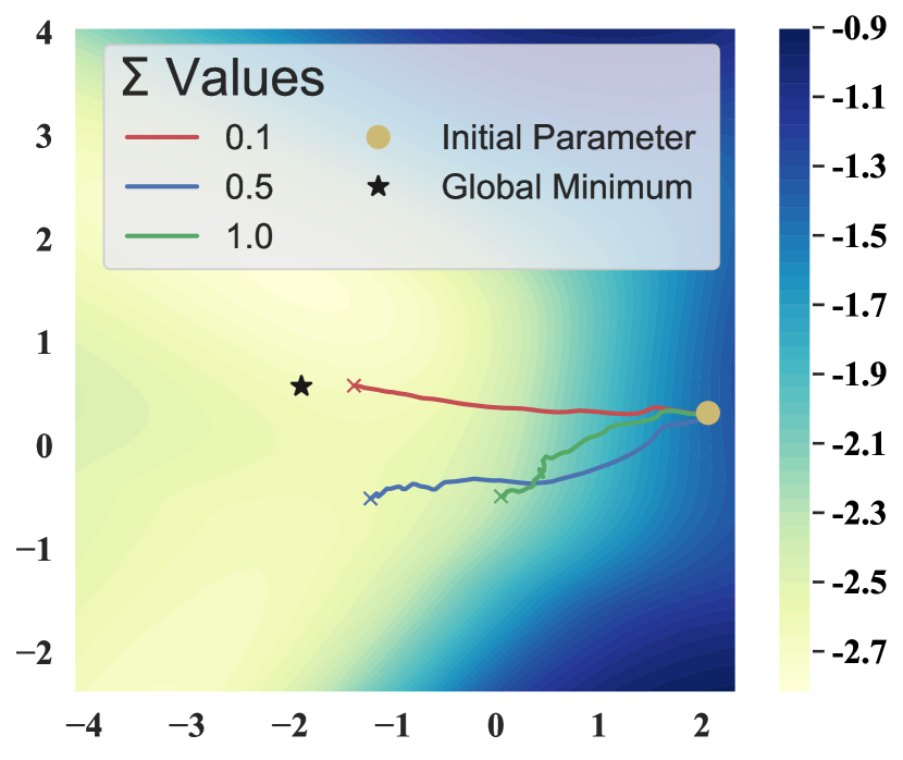
(a) Loss landscape for $\Sigma$

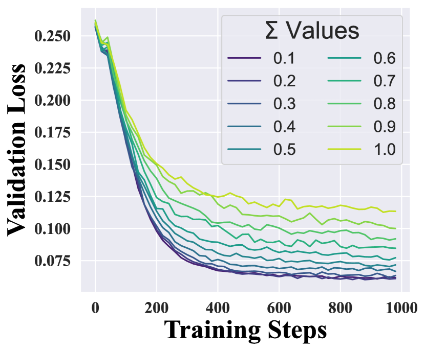
(b) Evaluate $G^{\prime}_{X}$ with different $\Sigma$

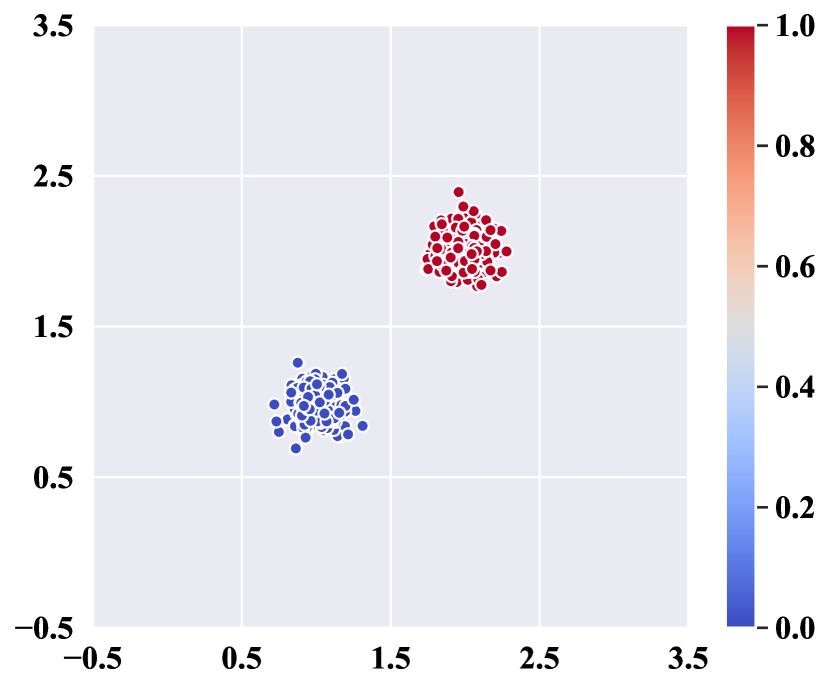
(c) Optimal $G^{\prime}_{X}$ ($\Sigma=0.1$)

Figure 1: Investigating distilled samples with varied $\Sigma$ values. Following Li et al. [37], Figure 1(a) visualizes the validation loss landscape within a two-dimensional parameter space, along with three training trajectories corresponding to different $\Sigma$ settings. Figure 1(b) illustrates the performance of models trained using samples with varied $\Sigma$. The optimal case in our task, utilizing samples with $\Sigma=0.1$ (which achieves the lowest validation loss in Figure 1(b)), is visualized in Figure 1(c), where the color bar represents the values of targets $y$.

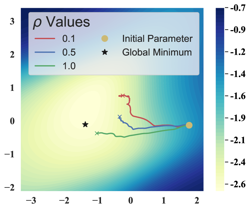
(a) Loss landscape for $\rho$

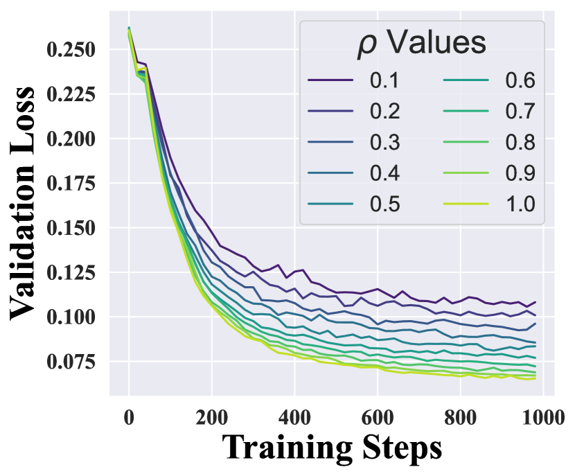
(b) Evaluate $G^{\prime}_{Y}$ with different $\rho$

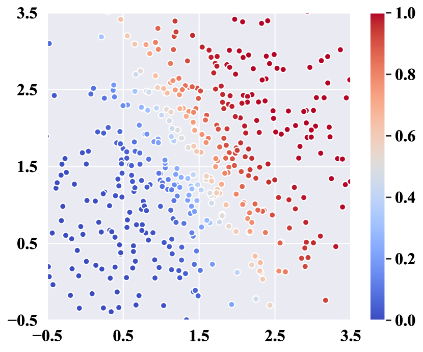
(c) Optimal $G^{\prime}_{Y}$ ($\rho=1.0$)

Figure 2: Investigating distilled targets with varied $\rho$ values. We present a visualization of the validation loss landscape in Figure 2(a), including three training trajectories that correspond to different $\rho$ settings. Figure 2(b) illustrates the performance of models trained using targets with varying $\rho$ values. The optimal scenario for our task, which uses targets with $\rho=1.0$, is depicted in Figure 2(c).

3.3 Extended Understanding of Data-centric Efficient Learning

The empirical and theoretical investigations on the properties of distilled samples $G^{\prime}_{X}$ and targets $G^{\prime}_{Y}$ in Section 3.2 are limited to a simplified case (as stated in Definition 4), and may not generalize to all practical scenarios such as training a ResNet [25] on the ImageNet dataset [20]. To extend our key insights to these scenarios, we conjecture a unified convergence rate for any distilled data $S$ below, which is theoretically correct for the cases of Definition 4 (see proof in Appendix C).

Conjecture 1

. For (self-)supervised learning tasks, the convergence rate for the model $\phi_{\boldsymbol{\theta}}$ trained after $t$ steps over $S$ (which contains any given $S_{X},S_{Y}$) is defined as (see Appendix C.1 for intuitions):

$$\textstyle{\mathbb{E}}_{\boldsymbol{\theta}_{t}}\left[{\mathcal{L}(\boldsymbol{\phi}_{\boldsymbol{\theta}_{t}};S;\ell)-\mathcal{L}(\boldsymbol{\phi}_{\boldsymbol{\theta}^{\star}};S;\ell)}\right]\leq\tilde{\mathcal{O}}(1-I_{\mathcal{O}}(S_{X},S_{Y}))\,,$$ (7)

where $I_{\mathcal{O}}(S_{X},S_{Y})\in[0,1]$ represents the normalized mutual information [50].

Theorem 3

(Normalized mutual information of $S_{X}$ and $S_{Y}$ from the perspective of labeler $\psi$) . For given $S_{X}$, labeler $\psi$, and $S_{Y}=\{\mathbf{y}\mid\mathbf{y}=\psi(\mathbf{x})\;\textup{s.t.}\;\mathbf{x}\sim S_{X}\}$, the normalized mutual information between $S_{X}$ and $S_{Y}$ is upper-bounded by that of $S_{X}$ and the optimal targets $S^{\star}_{Y}$:

$$I_{\mathcal{O}}(S_{X},S_{Y})\leq I_{\mathcal{O}}(S_{X},S^{\star}_{Y})=1\;\;\textup{s.t.}\;\;\exists\psi_{\star}^{-1}\in\Psi^{-1},\,{\mathbb{E}}_{(\mathbf{x},\mathbf{y})\sim S}\left[\mathbf{1}(\mathbf{x}\neq\psi_{\star}^{-1}(\mathbf{y}))\right]=0\,,$$ (8)

where $\psi_{\star}$ indicates the ideal labeler $\psi_{\star}$ for generating $S^{\star}_{Y}$, and $\psi_{\star}^{-1}$ denotes its inverse mapping.

Theorem 3 indicates that dataset generation, consisting of collecting samples $S_{X}$ and its targets $S_{Y}$, corresponds to find a labeler $\psi$ that maximizes $I_{\mathcal{O}}(S_{X},S_{Y})$, in which the discrepancy of ${\mathbb{E}}_{\boldsymbol{\theta}_{t}}\left[{\mathcal{L}(\boldsymbol{\phi}_{\boldsymbol{\theta}_{t}};S;\ell)-\mathcal{L}(\boldsymbol{\phi}_{\boldsymbol{\theta}^{\star}};S;\ell)}\right]$ in Conjecture 1 will be minimized and thus improves convergence. The ideal data can be achieved by approaching an ideal labeler $\psi_{\star}$ to establish the perfect bijective mapping between $S_{X}$ and $S_{Y}$ (namely enable $I_{\mathcal{O}}(S_{X},S_{Y})=1$).

However, real-world datasets often deviate from the ideal scenario described above, as discussed in Remark 1 below and further analyzed in Appendix O.

Remark 1

(Imperfect mappings and inaccurate targets in real-world datasets) . In practice, we observe that “noisy mappings” between input samples and targets are prevalent in real-world datasets. As illustrated in Figure 5, several common phenomena contribute to this issue:

• Similar or identical input samples may be assigned different targets due to using data augmentations, which is common in both self-supervised and human-supervised learning settings.

• Inaccurate targets may be generated, particularly in self-supervised learning scenarios.

• In human-supervised learning, all samples within a class are mapped to a one-hot encoded target.

These imperfect mappings and inaccurate targets pose challenges to achieving optimal training efficiency and effectiveness for real-world datasets.

4 Methodology

In this section, we complement previous analysis and derive generalization bounds for training models on the distilled dataset $S$. Building upon these theoretical insights, we propose our ReLA (see Figure 3): $\bullet$ ReLA-D () is used to generate distilled data (c.f. Sections 4.1); $\bullet$ ReLA-F () guides the models to train over the distilled data from ReLA-D () (c.f. Section 4.2).

Generalization-bounded data distillation paradigm. Given a labeler $\psi$, we articulate the generalization bound of models trained on the distilled dataset $S$ in Theorem 4 (c.f. Appendix E) below:

Theorem 4

(Generalization bound with labeler $\psi$) . Assumimg the model $\boldsymbol{\phi}_{\boldsymbol{\theta}}:\mathcal{X}\to\mathcal{Y}$ belongs to a hypothesis space $\Phi$. Then, for any $\delta\in(0,1)$, with probability at least $1-\delta$, we have

$$\textstyle\mathbb{E}_{\mathbf{x}\sim X}\left[\ell(\boldsymbol{\phi}_{\boldsymbol{\theta}}(\mathbf{x}),\psi(\mathbf{x}))\right]\leq\mathbb{E}_{\mathbf{x}\sim S_{X}}\left[\ell(\boldsymbol{\phi}_{\boldsymbol{\theta}}(\mathbf{x}),\psi(\mathbf{x}))\right]+\textup{D}_{\textup{TV}}(S_{X},D_{X})+\mathfrak{R}_{S_{X}}(\Phi)+\tilde{\mathcal{O}}(\frac{1}{\left\lvert S_{X}\right\rvert})\,,$$ (9)

where loss function is $\ell(\hat{y},y):=\mathbf{1}(\hat{y}\neq y)$, $\textup{D}_{\textup{TV}}$ represents the total variation divergence, and $\mathfrak{R}_{S_{X}}$ is the empirical Rademacher complexity.

Drawing all insights from Theorem 3 and 4, we define the properties of the ideal distilled data below:

Definition 5

(Properties of ideal distilled data, including samples $S_{X}$ and targets $S_{Y}$) . To meet the objectives of Definition 2 and 3 with a finite training budget, an ideal distilled data requires: ➀ generating targets $\psi(\mathbf{x})$ from the labeler $\psi$ that are accurate (i.e., align with human-annotating targets ) and informative (i.e., forming perfect bijective mappings with the original samples $\mathbf{x}$); ➁ low distribution disparity represented by $\textup{D}_{\textup{TV}}(S_{X},D_{X})$ and high sample diversity denoted as $\left\lvert S_{X}\right\rvert$.

4.1 ReLA-D (): Synthesis of Dynamic Dataset Distillation

Motivated by two property requirements in Definition 5, here we introduce our optimization-free synthesis process of both samples and targets in our ReLA-D (see technical details in Appendix H).

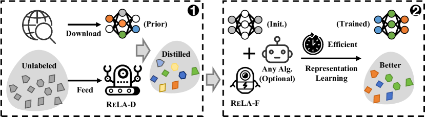
Figure 3: Framework of our ReLA, which comprises two primary components: 1) ReLA-D () operates as a distiller, utilizing an unlabeled dataset and a pre-trained model (e.g., a model obtained from online repositories) to generate a dynamic distilled dataset; 2) ReLA-F () functions as an auxiliary accelerator, enhancing existing self-supervised learning algorithms by leveraging the dynamic distilled dataset, thereby facilitating efficient representation learning. This procedure culminates in a well-trained model and provides an enhanced distilled dataset as an auxiliary benefit of ReLA.

Generating pseudo representations as the targets. We argue that well-trained models (called prior models) on diverse real-world datasets using various neural network architectures and algorithms converge towards the same linear representation space. In other words, the generated pseudo representations $R_{Y}$ for samples $D_{X}$ using these prior models are linearly transportable to each other and to the human-annotating targets. A formal statement can be found in Proposition 2 (c.f. Appendix H) and the empirical verifications refer to Section 5.1. We further theoretically justify in Appendix H.2 that the requirement ➀ in Definition 5 can be achieved by employing a prior model as the ideal labeler $\psi:\mathbb{R}^{d}\rightarrow\mathbb{R}^{m}$, i.e., generating $R_{Y}=\{\psi(\mathbf{x})\mid\mathbf{x}\sim D_{X}\}$ as the targets.

The generation process of targets is conducted only once (refer to Appendix J for details), and the generated targets $R_{Y}$ are stored and combined with the samples $D_{X}$ to form the dataset $D=(D_{X},R_{Y})$.

Efficient and distribution-aligned dynamic sample synthesis.

To meet the requirement ➁ in Definition 5 as well as achieve efficient learning with less computational burden during distillation, we utilize a simple yet zero-cost uniform random selection strategy to obtain diverse distilled samples (with associated generated targets stated above) per $k$-th epoch from $D=(D_{X},R_{Y})$, i.e., $S_{k}\sim D$.

4.2 ReLA-F (): Assist Learning with Dynamic Distilled Dataset

In this section, we showcase the significance of understanding ideal distilled data properties and dynamic dataset distillation in assisting self-supervised learning, given this self-supervised paradigm on unlabeled data suffers from significant inefficiency issues compared to human-supervised learning [61]. Yet, applying conventional self-supervised learning methods on the statically distilled samples $S_{X}$ is ineffective, leaving the benefits of targets $S_{Y}$ and dynamic dataset distillation untouched.

Here we propose a plug-and-play method that can be seamlessly integrated into any existing self-supervised learning algorithm, significantly enhancing its training efficiency by introducing an additional loss term. Formally, the loss function is defined as follows:

$$\lambda\cdot\mathcal{L}_{\textsc{ReLA}}(\boldsymbol{\phi}_{\boldsymbol{\theta}};(S_{X},S_{Y});\ell)+(1-\lambda)\cdot\mathcal{L}_{\texttt{SSL}}(\boldsymbol{\phi}_{\boldsymbol{\theta}};S_{X})\,,$$ (10)

where $\ell(\mathbf{x},\mathbf{y}):=1-{\mathbf{x}\cdot\mathbf{y}}/({\|\mathbf{x}\|\|\mathbf{y}\|})$ be the loss function, $\mathcal{L}_{\texttt{SSL}}$ denotes the loss specified by any self-supervised learning method, respectively. Furthermore, the data $S_{k}=(S_{X},S_{Y})$ are collected using the strategy outlined in Section 4.2, with updates occurring at each $k$-th epoch.

The dynamic coefficient $\lambda$ balances the two loss terms during training. Initially, $\lambda$ is set close to $1$ to emphasize $\mathcal{L}_{\textsc{ReLA}}$, assuming its crucial role in the early learning phase. As the model $\boldsymbol{\phi}_{\boldsymbol{\theta}}$ improves and self-generated targets become more reliable in $\mathcal{L}_{\texttt{SSL}}$, an adaptive attenuation algorithm decreases $\lambda$ in accordance (note that the initial $\lambda$ is tuning-free for all cases and see Appendix L for details).

To enhance the recognition of ReLA-aided algorithms, we re-denote those that are used in their names. For example, the BYOL algorithm [29], when enhanced with ReLA, is re-denoted as BYOL (). Furthermore, as the prior models downloaded from the internet are not consistently robust, the aforementioned dynamic setting of $\lambda$ also prevents the model $\boldsymbol{\phi}_{\boldsymbol{\theta}}$ from overfitting to potentially weak generated targets. The efficacy of our proposed ReLA is empirically validated in Section 5.

5 Experiments

This section describes the experimental setup and procedures undertaken to test our hypotheses and evaluate the effectiveness of our proposed methodologies.

Experimental setting.

We list the settings below (see more details in Appendix M).

$\bullet$ Datasets: For low-resolution data ($32\times 32$), we evaluate our method on two datasets, i.e., CIFAR-10 [34] and CIFAR-100 [33]. For high-resolution data, we conduct experiments on two large-scale datasets including Tiny-ImageNet ($64\times 64$) [35] and full ImageNet-1K ($224\times 224$) [20], to assess the scalability and effectiveness of our method on more complex and varied datasets.

$\bullet$ Neural network architectures: Similar to prior works/benchmarks of dataset distillation [55] and self-supervised learning [56, 19], we use several backbone architectures to evaluate the generalizability of our method, including ResNet-{18, 50, 101} [25], EfficientNet-B0 [57], MobileNet-V2 [49], ViT [21], and a series of CLIP-based models [46]. These architectures represent a range of model complexities and capacities, enabling a comprehensive assessment of our approach.

$\bullet$ Baselines: Referring to a prior widely-used benchmark [56, 19], we consider several state-of-the-art methods as baselines for a broader practical impact, including: SimCLR [12], Barlow Twins [67], BYOL [29], DINO [10], MoCo [26], SimSiam [13], SwAV [9], and Vicreg [3].

$\bullet$ Evaluation: Following previous benchmarks and research [56, 19, 12, 3], we evaluate all the trained models using offline linear probing strategy to reflect the representation ability of the trained models, and ensure a fair and comprehensive comparison with baseline approaches.

$\bullet$ Implementation details: We implement our method by extending a popular self-supervised learning open-source benchmark [56] and use their configurations therein. This includes using AdamW as the optimizer, with a mini-batch size of 128 (except for ImageNet-1K, where we use a mini-batch size of 256). We implement our method through PyTorch [45], and all experiments are conducted on NVIDIA RTX 4090 GPUs. See more detailed configurations and hyper-parameters in Appendix M.

Table 2: Benchmark our ReLA with various prior models against BYOL. We compare evaluation results of the models trained using $\bullet$ BYOL with $1\%$, $10\%$ and $20\%$ data; $\bullet$ BYOL () with different prior models; $\bullet$ BYOL with full data, denoted as BYOL^⋆ in this table. Regarding the prior models used for our ReLA, we respectively utilize six models with increasing representation capabilities, including $\bullet$ randomly initialized network (Rand.); $\bullet$ four BYOL^⋆-trained models (CF10-T, CF100-T, TIN-T, IN1K-T) corresponding to four datasets (listed below); $\bullet$ CLIP-RN50. The evaluations are performed across four datasets, i.e., CIFAR-10 (CF-10), CIFAR-100 (CF-100), Tiny-ImageNet (T-IN), and ImageNet-1K (IN-1K). We underline the results that outperform the full data training, and bold the results that achieve the highest performance using a specific ratio of data. All the networks used for training are ResNet-18, except the ResNet-50 used for IN-1K.

			BYOL () w/
Dataset	%	BYOL	Rand.	CF10-T	CF100-T	TIN-T	IN1K-T	CLIP-RN50	BYOL⋆
	1	39.8 $\pm$ 0.0	51.1 $\pm$ 0.2	54.1 $\pm$ 0.1	51.6 $\pm$ 0.0	52.5 $\pm$ 0.2	51.1 $\pm$ 0.2	52.4 $\pm$ 0.4
CF-10	10	56.1 $\pm$ 0.3	65.2 $\pm$ 0.1	80.8 $\pm$ 0.1	75.7 $\pm$ 0.1	78.5 $\pm$ 0.1	82.2 $\pm$ 0.1	83.2 $\pm$ 0.1	82.8 $\pm$ 0.1
	20	65.5 $\pm$ 0.2	75.2 $\pm$ 0.1	82.1 $\pm$ 0.1	80.7 $\pm$ 0.0	81.7 $\pm$ 0.0	84.2 $\pm$ 0.1	83.9 $\pm$ 0.2
	1	14.1 $\pm$ 0.4	24.1 $\pm$ 0.1	25.8 $\pm$ 0.2	25.3 $\pm$ 0.0	25.4 $\pm$ 0.1	24.9 $\pm$ 0.4	24.5 $\pm$ 0.2
CF-100	10	30.0 $\pm$ 0.3	36.7 $\pm$ 0.0	51.3 $\pm$ 0.0	52.1 $\pm$ 0.1	53.6 $\pm$ 0.2	55.6 $\pm$ 0.1	56.9 $\pm$ 0.1	51.7 $\pm$ 0.3
	20	33.1 $\pm$ 0.2	45.4 $\pm$ 0.2	54.0 $\pm$ 0.3	53.0 $\pm$ 0.1	56.4 $\pm$ 0.1	58.5 $\pm$ 0.1	57.0 $\pm$ 0.4
	1	8.5 $\pm$ 0.2	18.0 $\pm$ 0.2	21.4 $\pm$ 0.1	22.8 $\pm$ 0.3	24.4 $\pm$ 0.2	23.6 $\pm$ 0.1	20.7 $\pm$ 0.2
T-IN	10	26.4 $\pm$ 0.1	31.2 $\pm$ 0.5	35.8 $\pm$ 0.3	33.5 $\pm$ 0.0	39.0 $\pm$ 0.1	39.5 $\pm$ 0.1	42.2 $\pm$ 0.5	43.9 $\pm$ 0.2
	20	27.8 $\pm$ 0.2	34.6 $\pm$ 0.1	38.7 $\pm$ 0.1	39.0 $\pm$ 0.1	40.1 $\pm$ 0.1	42.3 $\pm$ 0.2	42.6 $\pm$ 0.4
	1	7.0 $\pm$ 0.1	18.3 $\pm$ 0.2	25.1 $\pm$ 0.1	23.3 $\pm$ 0.1	32.7 $\pm$ 0.2	33.9 $\pm$ 0.1	39.2 $\pm$ 0.2
IN-1K	10	45.2 $\pm$ 0.1	51.3 $\pm$ 0.1	52.9 $\pm$ 0.1	52.5 $\pm$ 0.0	53.3 $\pm$ 0.0	52.3 $\pm$ 0.0	52.6 $\pm$ 0.1	62.0 $\pm$ 0.0
	20	53.6 $\pm$ 0.1	54.6 $\pm$ 0.0	56.0 $\pm$ 0.0	56.0 $\pm$ 0.1	56.6 $\pm$ 0.0	56.5 $\pm$ 0.0	57.7 $\pm$ 0.0

5.1 Primary Experimental Results and Analysis

Recall that our ReLA-D (), as illustrated in Figure 3, requires an unlabeled dataset and any pre-trained model freely available online to generate the distilled dataset. To justify the superior performance and generality of our ReLA across various unlabeled datasets using prior models with different representation abilities, our comparisons in this subsection start with BYOL [29] and then extend to other self-supervised learning methods.

Table 2 demonstrates the efficacy and efficiency of our ReLA in facilitating the learning of robust representations. Overall, BYOL () consistently outperforms the original BYOL when trained on partial data. In certain cases, such as on CIFAR-100, BYOL () employing only $10\%$ of the data can surpass the performance of BYOL-trained models using the entire dataset. Specifically:

1. a stronger prior model (e.g., CLIP) enhances the performance of ReLA more effectively than a weaker model (e.g., Rand.);

2. our ReLA is not sensitive to the prior knowledge. For instance, using CF10-T as the prior model can achieve competitive performance compared to that trained on extensive datasets (e.g., CLIP);

3. a randomly initialized model can effectively aid in distilling the dataset through our ReLA. This can be considered an effective scenario of “weak-to-strong supervision” [7] using pseudo targets.

Cross-architecture generalization. ReLA-D () generates distilled datasets using a specific neural architecture. To evaluate the generalization ability of these datasets, it is essential to test their performance on various architectures not used in the distillation process. Table 3 presents the performance of our ReLA in conjunction with various prior models and trained model architectures, demonstrating its robust generalization ability. Specifically:

1. the integration of ReLA always enhances the performance of original BYOL;

2. our ReLA method exhibits minimal sensitivity to the architecture of the prior model, as evidenced by the comparable performance of BYOL () using both ViT-based and ResNet-based models.

Table 3: Evaluating our ReLA on cross-architecture settings. Our ReLA-D () distills datasets with prior CLIP-{RN50, RN101, RN50$\times$4, ViT B/32, ViT B/16, ViT L/14} and then versus transfer to ResNet-18; MobileNet-V2; EfficientNet-B0; ViT T/16. We train models over $10\%$ data through (original) BYOL ().

Dataset	Arch.	Original	() w/ RN50	RN101	RN50x4	ViT B/32	ViT B/16	ViT L/14
CF-10	ResNet-18	55.1 $\pm$ 0.2	83.2 $\pm$ 0.1	83.0 $\pm$ 0.1	83.8 $\pm$ 0.2	85.1 $\pm$ 0.0	85.3 $\pm$ 0.0	85.2 $\pm$ 0.1
	MobileNet-V2	41.8 $\pm$ 0.5	81.0 $\pm$ 0.2	83.5 $\pm$ 0.2	83.3 $\pm$ 0.1	85.7 $\pm$ 0.1	85.7 $\pm$ 0.1	84.2 $\pm$ 0.1
	EfficientNet-B0	23.8 $\pm$ 0.2	81.0 $\pm$ 0.2	85.0 $\pm$ 0.0	86.0 $\pm$ 0.1	87.2 $\pm$ 0.2	87.7 $\pm$ 0.0	87.4 $\pm$ 0.0
	ViT T/16	45.0 $\pm$ 0.3	63.9 $\pm$ 0.1	65.5 $\pm$ 0.1	64.2 $\pm$ 0.1	64.5 $\pm$ 0.0	65.0 $\pm$ 0.1	62.9 $\pm$ 0.1
T-IN	ResNet-18	25.3 $\pm$ 0.3	42.2 $\pm$ 0.5	40.3 $\pm$ 0.1	41.6 $\pm$ 0.3	42.4 $\pm$ 0.3	43.4 $\pm$ 0.1	41.9 $\pm$ 0.1
	MobileNet-V2	6.9 $\pm$ 0.2	33.0 $\pm$ 0.5	44.2 $\pm$ 0.4	40.8 $\pm$ 0.1	43.2 $\pm$ 0.2	42.4 $\pm$ 0.0	35.0 $\pm$ 0.1
	EfficientNet-B0	0.7 $\pm$ 0.1	41.8 $\pm$ 0.2	33.3 $\pm$ 0.1	39.8 $\pm$ 0.2	40.8 $\pm$ 0.1	48.4 $\pm$ 0.1	23.8 $\pm$ 0.2
	ViT T/16	14.9 $\pm$ 0.1	34.5 $\pm$ 0.2	32.7 $\pm$ 0.1	32.5 $\pm$ 0.2	31.7 $\pm$ 0.0	32.0 $\pm$ 0.2	29.3 $\pm$ 0.1

Combining ReLA across various self-supervised learning methods. To demonstrate the effectiveness and versatility of ReLA in enhancing various self-supervised learning methods, we conduct experiments with widely-used techniques. Table 4 presents the results, highlighting the robust generalization capability of ReLA. Our findings consistently show that ReLA improves the performance of these methods while maintaining the same data ratio, emphasizing its potential on learning using unlabeled data. Additionally, we provide the results when combining ReLA with human-supervised learning in Appendix K.

Table 4: Evaluating our ReLA across different self-supervised learning methods. We extend our analysis beyond BYOL by training and evaluating models using seven additional self-supervised learning methods, along with their ReLA-augmented counterparts (), utilizing randomly initialized ResNet-18 (Rand.) and CLIP-RN50 as prior models for the ReLA-D (). All methods are trained on a subset of $10\%$ of the full data.

Dataset	() w/	SimCLR	Barlow	DINO	MoCo	SimSiam	SwAV	Vicreg
CF-10	Original	71.2 $\pm$ 0.1	63.6 $\pm$ 0.0	64.1 $\pm$ 0.2	66.4 $\pm$ 0.1	50.0 $\pm$ 0.0	66.3 $\pm$ 0.4	68.7 $\pm$ 0.2
	Rand.	71.4 $\pm$ 0.3	65.5 $\pm$ 0.2	70.8 $\pm$ 0.2	71.2 $\pm$ 0.1	68.1 $\pm$ 0.2	72.4 $\pm$ 0.3	70.6 $\pm$ 0.2
	CLIP-RN50	82.1 $\pm$ 0.1	66.7 $\pm$ 0.2	80.5 $\pm$ 0.0	75.7 $\pm$ 0.2	85.1 $\pm$ 0.0	81.1 $\pm$ 0.2	74.6 $\pm$ 0.3
T-IN	Original	13.8 $\pm$ 0.3	28.3 $\pm$ 0.1	26.0 $\pm$ 0.3	27.7 $\pm$ 0.3	16.4 $\pm$ 0.5	18.4 $\pm$ 0.4	7.8 $\pm$ 0.2
	Rand.	31.8 $\pm$ 0.2	28.1 $\pm$ 0.3	31.4 $\pm$ 0.3	33.0 $\pm$ 0.1	30.8 $\pm$ 0.1	32.8 $\pm$ 0.2	31.9 $\pm$ 0.1
	CLIP-RN50	39.2 $\pm$ 0.3	28.4 $\pm$ 0.0	36.6 $\pm$ 0.1	35.1 $\pm$ 0.0	44.9 $\pm$ 0.2	41.5 $\pm$ 0.1	32.3 $\pm$ 0.0

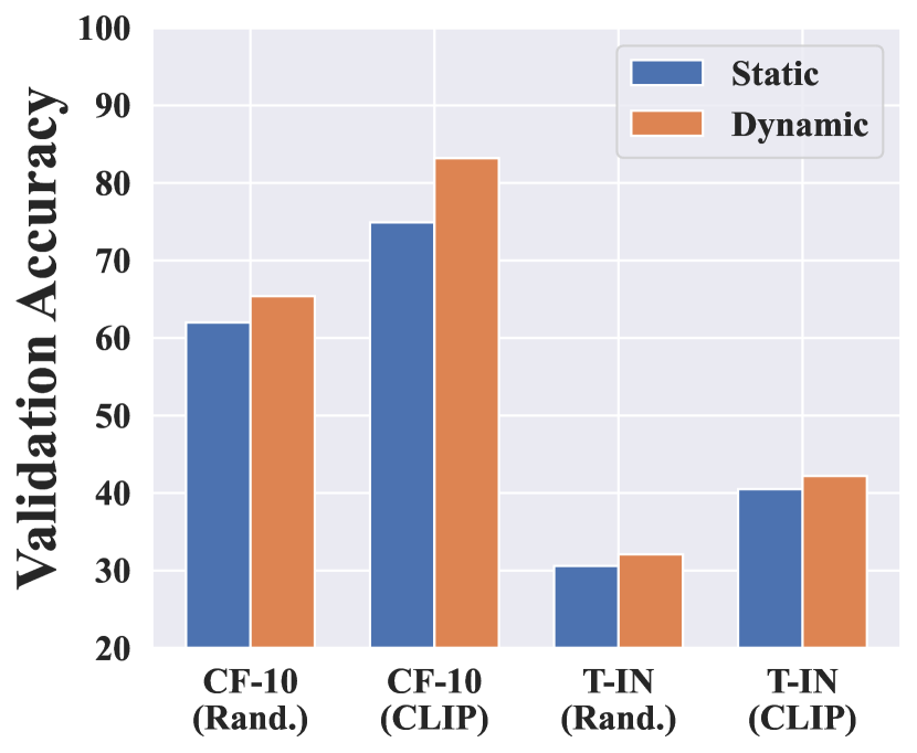
(a) Static vs. Dynamic distillation

(b) Value of constant $\lambda$

(c) Various ratios of data

Figure 4: Ablation study on BYOL () components and parameters. We replace the dynamic distilled dataset in BYOL () with a static one, using prior models such as Rand. and CLIP, and report the final performance of the trained models in Figure 4(a). Figure 4(b) shows the results of using different $\lambda$ values, where dotted ‘- -’ and solid ‘—’ lines denote our dynamic $\lambda$ and pre-set constant $\lambda$, respectively. We vary the ratio of distilled data used during training and report the results in Figure 4(c), with dotted ‘- -’ lines indicating the full data training accuracy.

5.2 Ablation Study

We conduct ablation studies to understand the impact of each component of ReLA on performance.

Dynamic vs. static dataset distillation. As the primary contribution of our ReLA algorithm, we propose and utilize a dynamic distilled dataset, where the data within each training epoch is dynamically updated in a zero-cost manner (see Section 4.1 for details). To establish a natural and zero-cost baseline, we compare our approach to a static strategy that ceases updates after the initial epoch. Figure 4(a) illustrates that employing a dynamic distilled dataset consistently surpasses the static strategy, achieving improvements ranging from $1.5\%$ to $8.3\%$.

Combining ReLA and BYOL with constant $\lambda$ setting strategies. The coefficient $\lambda$, introduced in Section 4.2, plays a crucial role in balancing the weights of the two loss terms, $\mathcal{L}_{\textsc{ReLA}}$ and $\mathcal{L}_{\texttt{SSL}}$. To evaluate the robustness of our adaptive strategy for dynamically setting $\lambda$ during the training procedure, we compare it against simply using static/constant $\lambda$ values. The results presented in Figure 4(b) demonstrate that larger (smaller) $\lambda$ values benefit the ReLA-D () more when using a strong (weak) prior model, respectively. However, these static settings cannot be generalized to various scenarios, while our adaptive strategy exhibits better generalization capabilities.

Sensitivity of ReLA to different distilled data ratios (over the original training data). We investigate the sensitivity of our proposed ReLA algorithm under varying ratios of training data, as illustrated in Figure 4(c). The results demonstrate that the performance of BYOL () exhibits a consistent improvement as the proportion of utilized data increases. Given sufficient data, BYOL () is capable of achieving and surpassing the accuracy obtained from training on the full dataset. We additionally examine the performance of BYOL (), using a ResNet-50 architecture and the prior CLIP-ViT B/16 model. Our experiment shows that training on only $50\%$ of the IN-1K data achieves an accuracy of $62.2\%$, surpassing the performance of original BYOL training on the full dataset (see Table 2).

6 Conclusion and Limitation

In this paper, we investigate the optimal properties of data, including samples and targets, to identify the properties that improve generalization and optimization in deep learning models. Our theoretical insights indicate that targets which are informative and linearly transportable to strong representations (e.g., human annotations) enable trained models to exhibit robust representation abilities. Furthermore, we empirically and theoretically find that well-trained models (called prior models) across various tasks and architectures serve as effective labelers for generating such targets. Consequently, we propose the Representation Learning Accelerator (ReLA), which leverages any freely available prior model to generate high-quality targets for samples. Additionally, ReLA can enhance existing (self-)supervised learning approaches by utilizing these generated data to accelerate training.

However, our theoretical analysis is confined to the simplified scenario outlined in Definition 4. The applicability of dataset distillation to more complex data distributions and larger models remains undetermined, and the existence of optimal data is still unknown. It is important to note that Conjecture 1 remains speculative. Furthermore, the linear transferability of representations generated by models trained on broader tasks (e.g., semantic segmentation, object detection) across different neural architectures necessitates both experimental and theoretical validation.

Appendix A Proof of Theorem 1

In this section, we prove a simplified case of 1 for technical reasons. Yet this proof could still reflect the essential of the theorem.

A.1 Setup

Notation N denotes the normal distribution, B for Bernoulli distribution.
We focus on the 1-dim situation. Assume that $\mu_{1}<\mu_{2}$. Define the original data distribution($\mathcal{N}_{0}=\textup{N}(\mu_{1},\Sigma^{2}_{0})$ and $\mathcal{N}_{1}=\textup{N}(\mu_{2},\Sigma^{2}_{0})$)

$$G:=\{(x,y)\mid y\sim 2\cdot\textup{B}(1,\frac{1}{2})-1,x\sim\frac{1-y}{2}\cdot\mathcal{N}_{0}+\frac{1+y}{2}\cdot\mathcal{N}_{1}\}$$

and the modified one ($\mathcal{N}_{0}^{\prime}=\textup{N}(\mu_{1},\Sigma^{2})$ and $\mathcal{N}_{1}^{\prime}=\textup{N}_{(}\mu_{2},\Sigma^{2})$):

$$G^{\prime}:=\{(x,y)\mid y\sim 2\cdot\textup{B}(1,\frac{1}{2})-1,x\sim\frac{1-y}{2}\cdot\mathcal{N}_{0}^{\prime}+\frac{1+y}{2}\cdot\mathcal{N}_{1}^{\prime}\}\,.$$

Our task is predicting $y$ given $x$. Note that $y\in\{\pm 1\}$, which is a bit different from the definition in Section 3.2. In 1-dim situation, we just need one parameter for this classification task, so define $f_{\theta}(x):=\textup{sign}(x+\theta)$ to fit the distribution. We could compute the generalization loss on original distribution:

$$\mathcal{L}(f_{\theta})=(\int_{-\theta}^{+\infty}\,dF_{-}+\int^{-\theta}_{-\infty}\,dF_{+})/2=(1-\int_{-\frac{\theta+\mu_{2}}{\Sigma_{0}}}^{-\frac{\theta+\mu_{1}}{\Sigma_{0}}}\,dF)/2$$

Obviously $\theta^{\star}=-\frac{\mu_{1}+\mu_{2}}{2}$, we have:

$$\mathcal{L}(f_{\theta})-\mathcal{L}(f_{\theta^{\star}}) =(\int_{-\frac{\mu_{2}-\mu_{1}}{2\Sigma_{0}}}^{\frac{\mu_{2}-\mu_{1}}{2\Sigma_{0}}}\,dF-\int_{-\frac{\theta+\mu_{2}}{\Sigma_{0}}}^{-\frac{\theta+\mu_{1}}{\Sigma_{0}}}\,dF)/2$$

$$\leq C_{1}\cdot(\theta-\theta^{\star})^{2}\quad(or\;C_{1}^{\prime}\,|\theta-\theta^{\star}|)$$

where $C_{1}$, $C_{1}^{\prime}$ are constants, $F_{0}$ $F_{1}$ $F$ denote the CDF of $\mathcal{N}_{0}$ $\mathcal{N}_{1}$ and the standard normal distribution respectively. The inequality above is due to the fact that function $h(x)=(\int^{1}_{-1}\,dF-\int_{x-1}^{x+1}\,dF)/x^{2}$ has limits at 0 and so is bounded.

A.2 Algorithm

For a dataset $\{(x_{i},y_{i})\}_{i=1}^{n}$, set the loss function $L(\theta)=\frac{1}{n}\sum_{i=1}^{n}\ell\left[y_{i}(x_{i}+\theta)\right]$, $\ell(v)=\tfrac{1}{2}(1-v)^{2}$. We apply the stocastic gradient descent algorithm and assume the online setting ($n=1$): at step $t$ draw one sample $(x_{t},y_{t})$ from $G^{\prime}$ then use the gradient $\nabla L(\theta_{t})$ to update $\theta$ ($\eta\in(0,1),t\in\mathbb{N}$):

$$\theta_{t+1}=\theta_{t}-\eta\nabla L(\theta_{t}),$$

$$\nabla L(\theta_{t})=\theta+(x_{t}-y_{t}).$$

It can be observed that randomness of $x$ leads to noies on gradient.

A.3 Bounds with $\Sigma$

We prove the proposition that lower $\Sigma$ can make convergence faster, i.e. ${\mathbb{E}}\left[\mathcal{L}(f_{\theta_{t}})-\mathcal{L}(f_{\theta^{\star}})\right]$ is bounded by an increasing function of $\Sigma$ ($t$ fixed).

Proof.

From above, we could get

$$\theta_{t}=(1-\eta)^{t}\theta_{0}-\eta\left[(x_{t-1}-y_{t-1})+(1-\eta)(x_{t-2}-y_{t-2})+\dots+(1-\eta)^{t-1}(x_{0}-y_{0})\right]$$

and so :

$${\mathbb{E}}\left[\mathcal{L}(f_{\theta_{t}})-\mathcal{L}(f_{\theta^{\star}})\right] \leq C_{1}{\mathbb{E}}\left[(\theta_{t}-\theta^{\star})^{2}\right]$$

$$=C_{1}{\mathbb{E}}\,\{\left[(1-\eta)^{t}(\theta_{0}-\theta^{\star})-\eta\sum_{j=1}^{t}(1-\eta)^{j-1}(x_{t-j}-y_{t-j}+\theta^{\star})\right]^{2}\}$$

$$=C_{1}{\mathbb{E}}\left[(1-\eta)^{2t}(\theta_{0}-\theta^{\star})^{2}+\eta^{2}\sum_{j=1}^{t}(1-\eta)^{2(j-1)}(x_{t-j}-y_{t-j}+\theta^{\star})^{2}\right]$$

$$=(1-\eta)^{2t}(C_{2}+C_{3}\Sigma^{2})$$

where $C_{2}=C_{1}\left[(\theta_{0}-\theta^{\star})^{2}+\frac{\eta}{(2-\eta)}(1-\frac{\mu_{2}-\mu_{1}}{2})^{2}\right]$, $C_{3}=C_{1}\frac{\eta}{2-\eta}$.
The last two equalities is due to the fact that for $(x,y)\sim G^{\prime}$

$${\mathbb{E}}\left[x-y+\theta^{\star}\right]=0\;,$$

$${\mathbb{E}}\left[(x-y+\theta^{\star})^{2}\right]=\Sigma^{2}+\left(1-\frac{\mu_{2}-\mu_{1}}{2}\right)^{2}.$$

∎

A.4 Nonlinear case

In this subsection, we conduct some qualitative analysis on the nonlinear case. The setting is the same as that in Section 3.2. We point out the differences compared with the linear case above: $\mathbf{x}\in\mathbb{R}^{d},y\in\{0,1\}$ and

$$\textstyle f_{\boldsymbol{\theta}}(\mathbf{x}):=\sigma\left(\boldsymbol{\theta}^{[1]}\cdot\textup{ReLU}\left(\boldsymbol{\theta}^{[2]}\mathbf{x}+\boldsymbol{\theta}^{[3]}\right)+\boldsymbol{\theta}^{[4]}\right)$$

where $\sigma(z)=\frac{1}{1+e^{-z}}$ is the sigmoid function; $\textup{ReLU}(z)=\max(0,z)$ is the activation function for the hidden layer, which provides non-linearity to the model; $\boldsymbol{\theta}^{[2]}$ and $\boldsymbol{\theta}^{[3]}$ are the weights and biases of the hidden layer; $\boldsymbol{\theta}^{[1]}$ and $\boldsymbol{\theta}^{[4]}$ are the weights and biases of the output layer.

To make things explicit, we still assume the online setting and set the loss function $L(\theta)=\frac{1}{2}(f_{\boldsymbol{\theta}}(\mathbf{x})-y)^{2}$. Assume after some iterations, $\boldsymbol{\theta}^{[2]}\cdot\mu_{1}+\boldsymbol{\theta}^{[3]}<0$ and $\boldsymbol{\theta}^{[2]}\cdot\mu_{2}+\boldsymbol{\theta}^{[3]}>0$ (coordinate-wise). In this situation, we could see that if $\mathbf{x}$ is close to its mean($\mu_{1}$ or $\mu_{2}$), the sign of $\textup{ReLU}\left(\boldsymbol{\theta}^{[2]}\mathbf{x}+\boldsymbol{\theta}^{[3]}\right)$ will be the same as $y$. So $f_{\boldsymbol{\theta}}$ will become an optimal classifier if $\boldsymbol{\theta}^{[1]}\to+\infty$ and $\boldsymbol{\theta}^{[4]}\to-\infty$. We focus on $\boldsymbol{\theta}^{[1]}$, using SGD:

$$\boldsymbol{\theta}^{[1]}_{t+1}=\boldsymbol{\theta}^{[1]}_{t}-\eta\frac{\partial L}{\partial\boldsymbol{\theta}^{[1]}},$$

$$\frac{\partial L}{\partial\boldsymbol{\theta}^{[1]}}=(f_{\boldsymbol{\theta}}(\mathbf{x})-y)\sigma(1-\sigma)\textup{ReLU}\left(\boldsymbol{\theta}^{[2]}\mathbf{x}+\boldsymbol{\theta}^{[3]}\right)$$

Note that we drop the variable value in $\sigma(\cdot)$ to make the expression more compact.

Then we can analyze the phenomenon qualitatively: larger $\Sigma$ will make convergence slower. The reason is that the larger $\Sigma$ is, when $\mathbf{x}$ is drawn from $\mathcal{N}_{1}$ ($y=1$), $\boldsymbol{\theta}^{[2]}\mathbf{x}+\boldsymbol{\theta}^{[3]}<0$ is more likely to happen(i.e. straying far away from the mean), causing $\boldsymbol{\theta}^{[1]}$ to stop updating; what’s worse, when $\mathbf{x}$ is drawn from $\mathcal{N}_{0}$ ($y=0$), with larger probability $\boldsymbol{\theta}^{[2]}\mathbf{x}+\boldsymbol{\theta}^{[3]}>0$ which will make $\boldsymbol{\theta}^{[1]}$ to go in the opposite direction. In summary, it is $\Sigma$ that makes the gradient noisy thus impacts the convergence rate.

Appendix B Proof of Theorem 2

B.1 Setting

Use the same setting in Section A(linaer case) except that

$$G^{\prime}:=\{(x,y^{\prime})\mid y\sim 2\cdot\textup{B}(1,\frac{1}{2})-1,x=\frac{1-y}{2}\cdot\mathcal{N}_{0}+\frac{1+y}{2}\cdot\mathcal{N}_{1},y^{\prime}=\rho\cdot f_{\theta^{*}}(x)+(1-\rho)y\}\,.$$

In other words, we modify the distribution of $y$ instead of $x$ this time.

B.2 Bounds with $\rho$

We’re gong to prove that higher $\rho$ can make convergence faster, i.e. ${\mathbb{E}}\left[\mathcal{L}(f_{\theta_{t}})-\mathcal{L}(f_{\theta^{\star}})\right]$ is bounded by an decreasing function of $\rho$ ($t$ fixed).

Proof.

The crucial part $x-y^{\prime}+\theta^{\star}=\rho(x-f_{\theta^{*}}(x)+\theta^{\star})+(1-\rho)(x-y+\theta^{\star})$, and in fact

$${\mathbb{E}}|x-y+\theta^{\star}|-{\mathbb{E}}|x-f_{\theta^{*}}(x)+\theta^{\star}|:=\epsilon_{0}>0\;.$$

Similarly, we can get bounds with $\rho$ (see $C_{1}^{\prime}$ in Section A):

$${\mathbb{E}}\left[\mathcal{L}(f_{\theta_{t}})-\mathcal{L}(f_{\theta^{\star}})\right] \leq C_{1}^{\prime}{\mathbb{E}}\left[(1-\eta)^{t}|\theta_{0}-\theta^{\star}|+(1-(1-\eta)^{t})|x-y^{\prime}+\theta^{\star}|\right]$$

$$\leq C_{2}(1-\eta)^{t}+C_{1}^{\prime}(1-(1-\eta)^{t})\left[\rho\cdot{\mathbb{E}}|x-f_{\theta^{*}}(x)+\theta^{\star}|\right.$$

$$\quad\left.+(1-\rho)\cdot{\mathbb{E}}|x-y+\theta^{\star}|\right]$$

$$\leq C_{2}(1-\eta)^{t}+(1-(1-\eta)^{t})(C_{3}-C_{4}\rho)$$

where $C_{2}=C_{1}^{\prime}\;|\theta_{0}-\theta^{\star}|$, $C_{3}=C_{1}^{\prime}\;{\mathbb{E}}|x-y+\theta^{\star}|$, $C_{4}=C_{1}^{\prime}\;\epsilon_{0}>0$. ∎

B.3 Nonlinear case

To see the impact of modifying $y$ more clearly, we directly set $\rho=1$ and conduct a similar analysis as in Section A.4. Let’s still focus on $\boldsymbol{\theta}^{[1]}$ and use the same assumptions in Section A.4, then we have:

$$\boldsymbol{\theta}^{[1]}_{t+1}=\boldsymbol{\theta}^{[1]}_{t}-\eta\frac{\partial L}{\partial\boldsymbol{\theta}^{[1]}},$$

$$\frac{\partial L}{\partial\boldsymbol{\theta}^{[1]}}=(f_{\boldsymbol{\theta}}(\mathbf{x})-f_{\boldsymbol{\theta}^{*}}(\mathbf{x}))\sigma(1-\sigma)\textup{ReLU}\left(\boldsymbol{\theta}^{[2]}\mathbf{x}+\boldsymbol{\theta}^{[3]}\right)$$

Note $y$ is replaced by $f_{\boldsymbol{\theta}^{*}}(\mathbf{x})$. For instance $\mathbf{x}$ is drawn from $\mathcal{N}_{0}$ ($y=0$) but strays far away from the $\mu_{1}$, causing $\boldsymbol{\theta}^{[2]}\mathbf{x}+\boldsymbol{\theta}^{[3]}>0$. In this situation $f_{\boldsymbol{\theta}^{*}}$ is likely to regard $\mathbf{x}$ as a sample from $\mathcal{N}_{1}$ (i.e. $f_{\boldsymbol{\theta}^{*}}(\mathbf{x})$ close to 1) thus making $\boldsymbol{\theta}^{[1]}$ to go in the right direction instead of the opposite. This explains why larger $\rho$ can make convergence faster.

Appendix C Proof of Conjecture 1

C.1 Intuition of Normalized Mutual Information

We poist that the noise within a dataset comes from the mismatch of information between samples and targets, e.g., the samples shown in Definition 4 are informative but their targets are uninformative, thus increasing the burden of learning the mapping function between them and hurting the learning efficiency. Therefore, based on the above conjecture, an reasonable solution to reduce such noise points to maximize the normalized mutual information [5] between the samples and corresponding targets, e.g., reducing the information in samples shown in Figure 1(c) and enhancing the information in targets shown Figure 2(c) (c.f. Appendix O for more explanations).

C.2 Entropy

In this section, we begin by introducing the fundamental concepts of information theory, including entropy, mutual information, and normalized mutual information, which are essential for understanding the mathematical foundations of machine learning and artificial intelligence.

For a discrete random variable $X$ with probability mass function $p(x)=\Pr\{X=x\},x\in\mathbf{X}$, where $\mathbf{X}$ is the set of possible values that $X$ can take, the entropy of $X$ is defined as:

$$H(X)=-\sum_{x\in\mathbf{X}}p(x)\log p(x)$$ (11)

Similarly, for a pair of discrete random variables $(X,Y)$ with joint probability mass function $p(x,y)$, their joint entropy is defined as:

$$H(X,Y)=-\sum_{x\in\mathbf{X}}\sum_{y\in\mathcal{Y}}p(x,y)\log p(x,y)$$ (12)

The conditional entropy $H(Y|X)$ represents the uncertainty of random variable $Y$ given that the value of random variable $X$ is known, and is defined as:

$$H(Y|X)=\sum_{x\in\mathbf{X}}p(x)H(Y|X=x)=-\sum_{x\in\mathbf{X}}\sum_{y\in\mathcal{Y}}p(x,y)\log p(y|x)$$ (13)

C.3 Mutual Information

The mutual information $I(X;Y)$ between two random variables $X$ and $Y$ is defined as:

$$I(X;Y)=\sum_{x\in\mathbf{X}}\sum_{y\in\mathcal{Y}}p(x,y)\log\frac{p(x,y)}{p(x)p(y)}$$ (14)

Mutual information can also be expressed in terms of entropy:

$$I(X;Y)=H(X)+H(Y)-H(X,Y)=H(X)-H(X|Y)=H(Y)-H(Y|X)$$ (15)

C.4 Normalized Mutual Information

The normalized mutual information $I_{\mathcal{O}}(X;Y)$ is defined as:

$$I_{\mathcal{O}}(X;Y)=\frac{2\cdot I(X;Y)}{H(Y)+H(X)}$$ (16)

Normalized mutual information takes values in the range $[0,1]$ and measures the statistical dependence between two random variables. If $X$ and $Y$ are independent, then $I_{\mathcal{O}}(X;Y)=0$; if $X$ and $Y$ are completely correlated, then $I_{\mathcal{O}}(X;Y)=1$. Normalized mutual information eliminates the influence of the range of variable values, making the mutual information between different pairs of variables comparable.

C.5 Normalized Mutual Information and Variance in Gaussian Mixture Distributions

In this section, we analyze the relationship between the normalized mutual information $I_{\mathcal{O}}(G_{X};G_{Y})$ and the variance $\Sigma^{2}$ in a bimodal Gaussian mixture distribution $G=(G_{X},G_{Y})$, which is defined as:

$$G:={(\mathbf{x},y)\mid\mathbf{x}=(1-y)\cdot\mathbf{x}_{0}+y\cdot\mathbf{x}_{1};\textup{s.t.};y\sim\textup{Bernoulli}(p=0.5),\mathbf{x}_{0}\sim\mathcal{N}_{0},\mathbf{x}_{1}\sim\mathcal{N}_{1}},,$$ (17)

where $\mathcal{N}_{0}(\mu_{1},\Sigma^{2})$ and $\mathcal{N}_{1}(\mu_{2},\Sigma^{2})$ are two Gaussian distributions with means $\mu_{1}$ and $\mu_{2}$, and a shared variance $\Sigma^{2}$.

We start by calculating the marginal entropy $H(G_{Y})$. Since $G_{Y}$ follows a Bernoulli distribution with $p=0.5$, we have:

$$H(G_{Y})=-\sum_{y\in{0,1}}p(y)\log p(y)=\log 2,.$$ (18)

Next, we compute the marginal entropy $H(G_{X})$. As $G_{X}$ is an equal-weighted mixture of two Gaussian distributions, we have:

$$H(G_{X})=-\int_{-\infty}^{\infty}p(x)\log p(x)dx=-0.5\int_{-\infty}^{\infty}(\mathcal{N}_{0}\log(0.5\mathcal{N}_{0})+\mathcal{N}_{1}\log(0.5\mathcal{N}_{1}))dx,.$$ (19)

Using the entropy formula for a univariate Gaussian distribution $H(\mathcal{N}(\mu,\sigma^{2}))=\frac{1}{2}\log(2\pi e\sigma^{2})$, we obtain:

$$H(G_{X})=\frac{1}{2}\log(2\pi e\Sigma^{2})+\log 2,.$$ (20)

Now, we calculate the conditional entropy $H(G_{X}|G_{Y})$. Given $Y$, $X$ follows a univariate Gaussian distribution:

$$p(x|y)=\begin{cases}\mathcal{N}_{0}(x;\mu_{1},\Sigma^{2}),&y=0\\ \mathcal{N}_{1}(x;\mu_{2},\Sigma^{2}),&y=1\end{cases},.$$ (21)

Therefore,

$$H(G_{X}|G_{Y})=\sum_{y\in{0,1}}p(y)H(G_{X}|G_{Y}=y)=\frac{1}{2}\log(2\pi e\Sigma^{2}),.$$ (22)

According to the definition of mutual information, we have:

$$I(G_{X};G_{Y})=H(G_{X})-H(G_{X}|G_{Y})=\log 2,.$$ (23)

Finally, the normalized mutual information is given by:

$$I_{\mathcal{O}}(G_{X};G_{Y})=\frac{2\cdot I(G_{X};G_{Y})}{H(G_{X})+H(G_{Y})}=\frac{2\log 2}{\frac{1}{2}\log(2\pi e\Sigma^{2})+2\log 2},.$$ (24)

The above equation provides the analytical relationship between the normalized mutual information $I_{\mathcal{O}}(G_{X};G_{Y})$ and the variance $\Sigma^{2}$. As $\Sigma$ decreases, $I_{\mathcal{O}}(G_{X};G_{Y})$ increases and eventually approaches 1. Conversely, as $\Sigma$ increases, $I_{\mathcal{O}}(G_{X};G_{Y})$ decreases and eventually approaches 0. This result is consistent with the qualitative analysis, demonstrating that a smaller variance leads to higher normalized mutual information in the given Gaussian mixture distribution.

C.6 Normalized Mutual Information and Targets in Gaussian Mixture Distributions

For the distributions in Definition 4, we can derive the following conditional probabilities and marginal probability:

$$p(\mathbf{x}|y=0) =\mathcal{N}(\mathbf{x}|\mu_{1},\Sigma^{2})$$ (25)

$$p(\mathbf{x}|y=1) =\mathcal{N}(\mathbf{x}|\mu_{2},\Sigma^{2})$$

$$p(y=0) =p(y=1)=0.5$$

When we construct a new $G_{Y}$ using $\hat{y}=\rho\cdot f_{\theta^{*}}(\mathbf{x})+(1-\rho)\cdot y$, we essentially replace the original $y$ with $\hat{y}$. If $f_{\theta^{*}}$ is a strong model that can provide correct and distinct predictions for any $\mathbf{x}$, then the normalized mutual information between $f_{\theta^{*}}(\mathbf{x})$ and $\mathbf{x}$ is 1, i.e.:

$$I_{\mathcal{O}}(\mathbf{x};f_{\theta^{*}}(\mathbf{x}))=1\Leftrightarrow I(\mathbf{x};f_{\theta^{*}}(\mathbf{x}))=H(\mathbf{x})=H(f_{\theta^{*}}(\mathbf{x}))$$ (26)

Next, let’s examine the change in normalized mutual information $I_{\mathcal{O}}(G_{X};G_{Y})$. By definition:

$$I_{\mathcal{O}}(G_{X};G_{Y})=\frac{2I(G_{X};G_{Y})}{H(G_{X})+H(G_{Y})}$$ (27)

When $\rho=0$, $\hat{y}=y$, and $I_{\mathcal{O}}(G_{X};G_{Y})$ is equal to the normalized mutual information of the original distribution $G$, denoted as $I_{\mathcal{O}}^{(0)}$.

As $\rho$ gradually increases to 1, we observe the change in $I_{\mathcal{O}}(G_{X};G_{Y})$:

$$\lim_{\rho\to 1}I_{\mathcal{O}}(G_{X};G_{Y}) =\lim_{\rho\to 1}\frac{2I(G_{X};G_{Y})}{H(G_{X})+H(G_{Y})}$$ (28)

$$=\frac{2\lim_{\rho\to 1}I(G_{X};G_{Y})}{\lim_{\rho\to 1}(H(G_{X})+H(G_{Y}))}$$

$$=\frac{2I(G_{X};f_{\theta^{*}}(G_{X}))}{H(G_{X})+H(f_{\theta^{*}}(G_{X}))}$$

$$=\frac{2H(G_{X})}{H(G_{X})+H(G_{X})}$$

$$=1$$

The third equality holds because:

$$\lim_{\rho\to 1}I(G_{X};G_{Y}) =\lim_{\rho\to 1}I(G_{X};\rho\cdot f_{\theta^{*}}(G_{X})+(1-\rho)\cdot G_{Y})$$ (29)

$$=I(G_{X};f_{\theta^{*}}(G_{X}))$$

$$=H(G_{X})$$

$$\lim_{\rho\to 1}H(G_{Y}) =\lim_{\rho\to 1}H(\rho\cdot f_{\theta^{*}}(G_{X})+(1-\rho)\cdot G_{Y})$$

$$=H(f_{\theta^{*}}(G_{X}))$$

$$=H(G_{X})$$

The last equality holds because $I_{\mathcal{O}}(\mathbf{x};f_{\theta^{*}}(\mathbf{x}))=1$.

In summary, we have proven that:

$$\lim_{\rho\to 1}I_{\mathcal{O}}(G_{X};G_{Y})=1>I_{\mathcal{O}}^{(0)}$$ (30)

This demonstrates that, under the given conditions, by constructing a new $G_{Y}$ using $\hat{y}=\rho\cdot f_{\theta^{*}}(\mathbf{x})+(1-\rho)\cdot y$, the normalized mutual information $I_{\mathcal{O}}(G_{X};G_{Y})$ gradually increases and approaches 1 as $\rho$ increases. Q.E.D.

Appendix D Proof of Theorem 3

We leverage the properties of mutual information and entropy. First, we introduce some notation and definitions.

Let $S_{X}$ denote the set of input samples, and let $S_{Y}$ denote the set of samples labeled by the labeler $\psi$, i.e., $S_{Y}=\{\mathbf{y}\mid\mathbf{y}=\psi(\mathbf{x})\;\textup{s.t.}\;\mathbf{x}\sim S_{X}\}$. Let $S^{\star}_{Y}$ denote the set of samples labeled by the ideal labeler $\psi_{\star}$.

The proof proceeds as follows:

By the definition of mutual information, we have:

$$I(S_{X};S_{Y})=H(S_{X})-H(S_{X}\mid S_{Y})$$ (31)

Since $S_{Y}$ is obtained by labeling $S_{X}$ with the labeler $\psi$, the uncertainty of $S_{X}$ given $S_{Y}$ decreases or remains the same, i.e.,

$$H(S_{X}\mid S_{Y})\leq H(S_{X})$$ (32)

Substituting this inequality into the previous equation, we get:

$$I(S_{X};S_{Y})\leq H(S_{Y})$$ (33)

Similarly, for the ideal labeler $\psi_{\star}$ and $S^{\star}_{Y}$, we have:

$$I(S_{X};S^{\star}_{Y})=H(S_{X})-H(S_{X}\mid S^{\star}_{Y})$$ (34)

Since $\psi_{\star}$ is the ideal labeler, there exists its inverse mapping $\psi_{\star}^{-1}$ such that $\mathbb{E}_{(\mathbf{x},\mathbf{y})\sim S}\left[\mathbf{1}(\mathbf{x}\neq\psi_{\star}^{-1}(\mathbf{y}))\right]=0$, i.e., given $\mathbf{y}\in S^{\star}_{Y}$, $\mathbf{x}\in S_{X}$ can be determined. Thus,

$$H(S_{X}\mid S^{\star}_{Y})=0$$ (35)

Substituting this equation into the previous equation, we get:

$$I(S_{X};S^{\star}_{Y})=H(S_{X})$$ (36)

By the definition of normalized mutual information, we have:

$$I_{\mathcal{O}}(S_{X},S_{Y})=\frac{2\cdot I(S_{X};S_{Y})}{H(S_{Y})+H(S_{X})}\leq\frac{2\cdot H(S_{Y})}{H(S_{Y})+H(S_{X})}\leq 1$$ (37)

where the first inequality follows from the earlier result, and the second inequality follows because $H(S_{Y})\leq H(S_{Y})+H(S_{X})$.

For the ideal labeler $\psi_{\star}$ and $S^{\star}_{Y}$, we have:

$$I_{\mathcal{O}}(S_{X},S^{\star}_{Y})=\frac{2\cdot I(S_{X};S^{\star}_{Y})}{H(S^{\star}_{Y})+H(S_{X})}=\frac{2\cdot H(S_{X})}{H(S^{\star}_{Y})+H(S_{X})}=1$$ (38)

where the first equality follows from the earlier result, and the second equality follows because $H(S^{\star}_{Y})=H(S_{X})$ (since $\psi_{\star}$ is a bijective function).

In summary, we have proven that:

$$I_{\mathcal{O}}(S_{X},S_{Y})\leq I_{\mathcal{O}}(S_{X},S^{\star}_{Y})=1\quad\textup{s.t.}\quad\exists\psi_{\star}^{-1}\in\Psi^{-1},\,\mathbb{E}_{(\mathbf{x},\mathbf{y})\sim S}\left[\mathbf{1}(\mathbf{x}\neq\psi_{\star}^{-1}(\mathbf{y}))\right]=0$$ (39)

Thus, Theorem 3 is proven.

Appendix E Proof of Theorem 4

We follow some proof steps in [4]. Let’s begin by introducing some notations used in this section.
Notation and Setup $\mathcal{X}$ is the input space, $\mathcal{D}_{S}$ and $\mathcal{D}_{T}$ are two distributions over $\mathcal{X}$. Let $\mathcal{Y}=\{0,1\}$. $\mathcal{H}$ denotes a hypothesis class from $\mathcal{X}$ to $\mathcal{Y}$. To simplify notations, $\forall h,f\in\mathcal{H}$ let $\epsilon_{S}(h,f)=E_{\mathbf{x}\sim\mathcal{D}_{S}}[\mathbf{1}(h(\mathbf{x})\neq f(\mathbf{x}))]$, and $\hat{\epsilon}_{S}(h,f)$ be empirical error ($\epsilon_{T}(h,f)$, $\hat{\epsilon}_{T}(h,f)$ similar).

Then we introduce some concepts and lemmas, most of which are from [4].

Definition 6 ($\mathcal{H}$-divergence)

The $\mathcal{H}$-divergence between two distributions $\mathcal{D}$ and $\mathcal{D}^{\prime}$ is defined as:

$$d_{\mathcal{H}}(\mathcal{D},\mathcal{D}^{\prime})=2\sup_{h\in\mathcal{H}}|\textup{Pr}_{\mathcal{D}}[I(h)]-\textup{Pr}_{\mathcal{D}^{\prime}}[I(h)]|$$

where $I(h)=\{\mathbf{x}:h(\mathbf{x})=1\}$.

Definition 7 (Total Variation Distance)

For two distributions $\mathcal{D}$ and $\mathcal{D}^{\prime}$, the total variation distance of them is defined as:

$$\textup{D}_{\textup{TV}}(\mathcal{D},\mathcal{D}^{\prime})=\sup_{A\subseteq\mathcal{F}}|\textup{Pr}_{\mathcal{D}}(A)-\textup{Pr}_{\mathcal{D}^{\prime}}(A)|$$

where $\mathcal{F}$ denotes the collection of all events in the probability space.

Lemma 1

For two distributions $\mathcal{D}$ and $\mathcal{D}^{\prime}$, by definition it’s easy to see that:

$$\frac{1}{2}d_{\mathcal{H}}(\mathcal{D},\mathcal{D}^{\prime})\leq\textup{D}_{\textup{TV}}(\mathcal{D},\mathcal{D}^{\prime})$$

Definition 8 (Symmetric Difference Hypothesis Space)

$$\mathcal{H}\Delta\mathcal{H}:=\{g:\mathcal{X}\to\{0,1\}|g(\mathbf{x})=h(\mathbf{x})\oplus h^{\prime}(\mathbf{x})\quad\forall h,h^{\prime}\in\mathcal{H}\}$$

$\oplus$ denotes the XOR operation.

Lemma 2

$$\forall h,h^{\prime}\in\mathcal{H},\left|\epsilon_{S}\left(h,h^{\prime}\right)-\epsilon_{T}\left(h,h^{\prime}\right)\right|\leq\frac{1}{2}d_{\mathcal{H}\Delta\mathcal{H}}\left(\mathcal{D}_{S},\mathcal{D}_{T}\right)$$

Proof.

only need note that $h(\mathbf{x})\oplus h^{\prime}(\mathbf{x})=|h(\mathbf{x})-h^{\prime}(\mathbf{x})|$, so

$$\sup_{g\in\mathcal{H}\Delta\mathcal{H}}|\textup{Pr}_{\mathcal{D}_{S}}[I(g)]-\textup{Pr}_{\mathcal{D}_{T}}[I(g)]|=\sup_{h,h^{\prime}\in\mathcal{H}}|\epsilon_{S}\left(h,h^{\prime}\right)-\epsilon_{T}\left(h,h^{\prime}\right)|$$

this is done by definition. ∎

Definition 9 (Rademacher complexity of a function class)

Given a sample of points $S=\{z_{1},z_{2},\ldots,z_{m}\}\subset Z$, and considering a function class $\mathcal{F}$ of real-valued functions over $Z$, the empirical Rademacher complexity of $\mathcal{F}$ given $S$ is defined as:

$$\mathfrak{R}_{S}(\mathcal{F})=\frac{1}{m}\mathbb{E}_{\sigma}\left[\sup_{f\in\mathcal{F}}\sum_{i=1}^{m}\sigma_{i}f(z_{i})\right]$$

where $\sigma_{i}$ are independent and identically distributed Rademacher random variables. In other words, for $i=1,2,\ldots,m$, the probability that $\sigma_{i}=+1$ is equal to the probability that $\sigma_{i}=-1$, and both are $\frac{1}{2}$.

Lemma 3 (Generalization bound with Rademacher complexity)

Let $\mathcal{F}$ be a family of loss functions $\mathcal{F}=\{(x,y)\mapsto\ell((x,y),h):h\in\mathcal{H}\}$ with $\ell((x,y),h)\in[0,1]$ for all $\ell,(x,y)$ and $h$. Then, with probability $1-\delta$, the generalization gap is

$${L}(h)-\hat{L}(h)\leq 2\mathfrak{R}_{U}(\mathcal{F})+3\sqrt{\frac{\log(2/\delta)}{2n}}\,,$$

for all $h\in\mathcal{H}$ and samples $U$ of size $n$.

The proof of this classical result could be found in most machine learning textbooks, like [43].

Now we are ready to prove a more general form of Theorem 4.

Proposition 1

Assumimg $\mathcal{H}$ is a hypothesis class from $\mathcal{X}$ to $\mathcal{Y}$ and $\boldsymbol{\phi},\boldsymbol{\phi}^{\prime}\in\mathcal{H}$. $U_{S}$ are samples of size $m$ drawn from the probability measure $D_{S}$. Then, for any $\delta\in(0,1)$, with probability at least $1-\delta$, we have

$$\mathbb{E}_{\mathbf{x}\sim\mathcal{D}_{T}}\left[\ell(\boldsymbol{\phi}(\mathbf{x}),\boldsymbol{\phi}^{\prime}(\mathbf{x}))\right]\leq\mathbb{E}_{\mathbf{x}\sim U_{S}}\left[\ell(\boldsymbol{\phi}(\mathbf{x}),\boldsymbol{\phi}^{\prime}(\mathbf{x}))\right]+\textup{D}_{\textup{TV}}(\mathcal{D}_{S},\mathcal{D}_{T})+2\mathfrak{R}_{U_{S}}(\mathcal{H})+\tilde{O}(\sqrt{\frac{\log(2/\delta)}{m}})$$

where loss function is $\ell(\hat{y},y):=\mathbf{1}(\hat{y}\neq y)$, and $\mathfrak{R}_{U_{S}}$ is the empirical Rademacher complexity.

Proof.

using the lemmas above and with probability $1-\delta$ at last step:

$$\epsilon_{T}(\boldsymbol{\phi},\boldsymbol{\phi}^{\prime}) \leq\epsilon_{S}\left(\boldsymbol{\phi},\boldsymbol{\phi}^{\prime}\right)+\left|\epsilon_{T}\left(\boldsymbol{\phi},\boldsymbol{\phi}^{\prime}\right)-\epsilon_{S}\left(\boldsymbol{\phi},\boldsymbol{\phi}^{\prime}\right)\right|$$

$$\leq\epsilon_{S}\left(\boldsymbol{\phi},\boldsymbol{\phi}^{\prime}\right)+\frac{1}{2}d_{\mathcal{H}\Delta\mathcal{H}}\left(\mathcal{D}_{S},\mathcal{D}_{T}\right)$$

$$\leq\epsilon_{S}\left(\boldsymbol{\phi},\boldsymbol{\phi}^{\prime}\right)+\textup{D}_{\textup{TV}}(\mathcal{D}_{S},\mathcal{D}_{T})$$

$$\leq\hat{\epsilon}_{S}(\boldsymbol{\phi},\boldsymbol{\phi}^{\prime})+\textup{D}_{\textup{TV}}(\mathcal{D}_{S},\mathcal{D}_{T})+2\mathfrak{R}_{U_{S}}(\ell\circ\mathcal{H})+\tilde{O}(\sqrt{\frac{\log(2/\delta)}{m}})$$

∎

Appendix F Conventional Dataset Distillation is Implicit Dynamic Dataset Distillation

Data augmentation is a common technique used to artificially increase the diversity of a training dataset by applying various transformations (e.g., rotations, scaling, translations, etc.) to the original data, which is also widely used for distilled dataset [55, 65, 64]. Let us denote the original static distilled dataset by $S$ and the augmented dataset by $S_{\text{Aug}}$.

For each original data point $(\mathbf{x}_{i},y_{i})\in S$, data augmentation generates a set of augmented samples:

$$\mathcal{A}(\mathbf{x}_{i})=\{\mathbf{x}_{i}^{(1)},\mathbf{x}_{i}^{(2)},\ldots,\mathbf{x}_{i}^{(m)}\}$$

where $\mathcal{A}$ denotes the augmentation process, and $m$ is the number of augmented samples generated from $\mathbf{x}_{i}$.

The augmented dataset $S_{\text{Aug}}$ can be expressed as:

$$S_{\text{Aug}}=\bigcup_{i=1}^{|S|}\mathcal{A}(\mathbf{x}_{i})$$

During training, the model iteratively uses different augmented versions of the data points in $S_{\text{Aug}}$. Thus, although the original distilled dataset $S$ remains static, the actual data seen by the model changes dynamically in each epoch due to augmentation. This introduces a form of implicit dynamic data into the training process. To formalize this, let’s consider the optimization objective with data augmentation. The empirical loss over the augmented dataset can be written as:

$$\boldsymbol{\theta}^{S_{\text{Aug}}}:=\operatorname*{arg\,min\,}_{\boldsymbol{\theta}\in\boldsymbol{\Theta}}\left\{\sum_{i=1}^{|S|}\sum_{j=1}^{m}\ell(\boldsymbol{\phi}_{\boldsymbol{\theta}}(\mathbf{x}_{i}^{(j)}),y_{i})\right\}$$

Comparing this with the static dataset distillation:

$$\boldsymbol{\theta}^{S}:=\operatorname*{arg\,min\,}_{\boldsymbol{\theta}\in\boldsymbol{\Theta}}\left\{\sum_{j=1}^{|\mathcal{S}|}\ell(\boldsymbol{\phi}_{\boldsymbol{\theta}}(\mathbf{x}_{j}),y_{j})\right\}$$

The key difference is that in the case of static data with augmentation, the data points $\mathbf{x}_{i}^{(j)}$ are dynamically generated and used in each training epoch, making the training data effectively dynamic.

Therefore, even though the original dataset $S$ is static, the use of data augmentation during training creates an implicit dynamic dataset $S_{\text{Aug}}$, aligning it with the concept of dynamic data in practice.

$$\boxed{\text{Implicitly, practically used }S_{\text{Aug}}\text{ is a dynamic dataset derived from the static distilled dataset }S.}$$

In contrast, our Definition 1 of dynamic dataset distillation can provide a direct way to utilize different $S_{k}$ in each epoch, where we can use more ways to capture data (instead of only using data augmentation).

Appendix G Explanation of Rescaling Samples

Dataset distillation seeks to create a condensed dataset that allows models to achieve performance comparable to those trained on the full dataset, but with fewer training steps. In this section, we will demonstrate that rescaling the variance of Gaussian distributions, as defined in Definition 4, does not affect the optimal performance of models trained on these rescaled data.

Proof.

Consider two Gaussian distributions $\mathcal{N}_{0}(\mu_{1},\sigma^{2}\mathbf{I})$ and $\mathcal{N}_{1}(\mu_{2},\sigma^{2}\mathbf{I})$ with means $\mu_{1}=1$ and $\mu_{2}=2$, and variance $\sigma^{2}$. We define the bimodal mixture distribution $G=(G_{X},G_{Y})$ such that $(\mathbf{x},y)$ is sampled according to:

$$\mathbf{x}=(1-y)\cdot\mathbf{x}_{0}+y\cdot\mathbf{x}_{1},\quad\text{with}\quad y\sim\text{Bernoulli}(0.5),\quad\mathbf{x}_{0}\sim\mathcal{N}_{0},\quad\mathbf{x}_{1}\sim\mathcal{N}_{1}.$$

The decision rule for optimal classification is determined by the likelihood ratio test. For a given sample $\mathbf{x}$, the log-likelihood ratio $\Lambda(\mathbf{x})$ is given by:

$$\Lambda(\mathbf{x})=\log\frac{P(\mathbf{x}\mid y=1)}{P(\mathbf{x}\mid y=0)}.$$

Since $\mathbf{x}_{0}$ and $\mathbf{x}_{1}$ are drawn from Gaussian distributions, their probability density functions are:

$$P(\mathbf{x}\mid y=0)=\frac{1}{(2\pi\sigma^{2})^{d/2}}\exp\left(-\frac{1}{2\sigma^{2}}\|\mathbf{x}-\mu_{1}\|^{2}\right),$$

$$P(\mathbf{x}\mid y=1)=\frac{1}{(2\pi\sigma^{2})^{d/2}}\exp\left(-\frac{1}{2\sigma^{2}}\|\mathbf{x}-\mu_{2}\|^{2}\right).$$

Substituting these into the log-likelihood ratio, we have:

$$\Lambda(\mathbf{x})=\log\frac{\frac{1}{(2\pi\sigma^{2})^{d/2}}\exp\left(-\frac{1}{2\sigma^{2}}\|\mathbf{x}-\mu_{2}\|^{2}\right)}{\frac{1}{(2\pi\sigma^{2})^{d/2}}\exp\left(-\frac{1}{2\sigma^{2}}\|\mathbf{x}-\mu_{1}\|^{2}\right)}.$$

Simplifying, we obtain:

$$\Lambda(\mathbf{x})=-\frac{1}{2\sigma^{2}}\|\mathbf{x}-\mu_{2}\|^{2}+\frac{1}{2\sigma^{2}}\|\mathbf{x}-\mu_{1}\|^{2}.$$

Further simplification gives:

$$\Lambda(\mathbf{x})=\frac{1}{2\sigma^{2}}\left(\|\mathbf{x}-\mu_{1}\|^{2}-\|\mathbf{x}-\mu_{2}\|^{2}\right).$$

Since the optimal decision threshold for balanced classes (i.e., $P(y=1)=P(y=0)=0.5$) is $\Lambda(\mathbf{x})=0$, we set:

$$\|\mathbf{x}-\mu_{1}\|^{2}-\|\mathbf{x}-\mu_{2}\|^{2}=0.$$

Expanding and rearranging, we derive:

$$\|\mathbf{x}-1\|^{2}=\|\mathbf{x}-2\|^{2}.$$

This simplifies to:

$$(x-1)^{2}=(x-2)^{2}.$$

Solving yields:

$$x^{2}-2x+1=x^{2}-4x+4.$$

Thus:

$$-2x+1=-4x+4,$$

$$2x=3,$$

$$x=\frac{3}{2}.$$

Therefore, the optimal decision boundary is $x=1.5$, which is independent of the variance $\sigma^{2}$. This completes the proof. ∎

Regarding efficiency, utilizing scaled data to train similar models with fewer training steps is proven in Section A. Additionally, rescaling each Gaussian distribution preserves their means, which aligns with the objectives of conventional distribution matching-based dataset distillation methods. These methods aim to distill data while maintaining the distributional properties, specifically their means.

Appendix H Detailed Methodology of ReLA-D

H.1 Synthesis of Samples Using ReLA-D.

Proposition 2

(Linear transportability of pseudo representations) . Given any two prior models $\xi(\cdot),\zeta(\cdot)\in\mathbb{R}^{m}$ (e.g., CLIP [46] and LVM [2]), the following holds:

$$D_{\mathbf{Y}}\!=\!\mathbf{W}_{(\xi\to\mathbf{Y})}\xi(D_{\mathbf{X}}),\;\xi(D_{\mathbf{X}})\!=\!\mathbf{W}_{(\zeta\to\xi)}\zeta(D_{\mathbf{X}})\;\;\textup{s.t.}\;\;\exists\mathbf{W}_{(\xi\to\mathbf{Y})}\!\in\!\mathbb{R}^{n\times m},\mathbf{W}_{(\zeta\to\xi)}\!\in\!\mathbb{R}^{m\times m}\,,$$ (40)

where $\mathbf{W}_{(\xi\to\mathbf{Y})}$ and $\mathbf{W}_{(\zeta\to\xi)}$ are two transport matrixs, $D_{\mathbf{Y}}$ and $D_{\mathbf{X}}$ are the matrix versions of $D_{Y}$ and $D_{X}$.

Recall that $\boldsymbol{\phi}_{\boldsymbol{\theta}}:\mathbb{R}^{d}\rightarrow\mathbb{R}^{n}$. We then introduce a transport matrix $\mathbf{W}\in\mathbb{R}^{m\times n}$ and define the combined model as $\mathbf{W}\boldsymbol{\phi}_{\boldsymbol{\theta}}(\cdot)\in\mathbb{R}^{m}$. During the training phase, the parameters $\mathbf{W}$ and $\boldsymbol{\theta}$ are jointly optimized. However, as the dimension $m$ increases, the computational complexity of the optimization grows rapidly. To address this issue, we propose reducing the dimensionality of the target matrix $R_{\mathbf{Y}}$ from $m$ to $n$, where $n<m$:

$$R_{\mathbf{Y}}^{\prime}\!=\!V_{n}^{\top}\left(\frac{R_{\mathbf{Y}}-\mu}{\sigma}\right)\;\;\textup{s.t.}\;\;\frac{1}{\left\lvert R_{\mathbf{Y}}\right\rvert-1}\left((R_{\mathbf{Y}}-\mu)^{\top}(R_{\mathbf{Y}}-\mu)\right)=V\Lambda V^{\top},\;V_{n}=V[:,:n]\,,$$ (41)

where $\mu$ and $\sigma$ denote the mean and standard deviation, respectively, of each column in the $R_{\mathbf{Y}}$. Practically, we use batch PCA to perform the computation shown in (41), as illustrated in Appendix N.

Theorem 5

(Bound of normalized mutual information of dimension-reduced targets) . For given $R_{\mathbf{Y}}$ and the reduced version of this as $R_{\mathbf{Y}}^{\prime}$, we have the bound of normalized mutual information:

$$I_{\mathcal{O}}(R_{\mathbf{Y}},R_{\mathbf{X}})\geq I_{\mathcal{O}}(R_{\mathbf{Y}}^{\prime},R_{\mathbf{X}})\;\textup{s.t.}\;R_{\mathbf{X}}=\{\mathbf{W}\boldsymbol{\phi}_{\boldsymbol{\theta}}(\mathbf{x})\mid\mathbf{x}\sim D_{X}\}\,.$$ (42)

Additionally, Theorem 5 provides a theoretical guarantee for the harmless of using (41) for efficacy.

H.2 Proof for Ideal Properties of Prior Models

According to Theorem 3, a prior model that can losslessly extract $D_{\mathbf{X}}$ qualifies as an ideal prior labeler, and then the requirement ➀ in Definition 5 can be achieved.

At first, by the Proposition 2, we can conclude that if there exists one prior model that can losslessly extract $D_{\mathbf{X}}$, then all prior models in the set can losslessly extract $D_{\mathbf{X}}$.

Proof.

1) Assume that there exists a model $\xi(\cdot)$ that can losslessly extract $D_{\mathbf{X}}$, i.e., there exists an inverse function $\xi^{-1}(\cdot)$ such that $D_{\mathbf{X}}=\xi^{-1}(\xi(D_{\mathbf{X}}))$.

2) From the Proposition 2, we have $\xi(D_{\mathbf{X}})=\mathbf{W}_{(\zeta\to\xi)}\zeta(D_{\mathbf{X}})$, which implies:

$$D_{\mathbf{X}}=\xi^{-1}(\xi(D_{\mathbf{X}}))=\xi^{-1}(\mathbf{W}_{(\zeta\to\xi)}\zeta(D_{\mathbf{X}}))$$

3) Let $\zeta^{-1}(\cdot)=\xi^{-1}(\mathbf{W}_{(\zeta\to\xi)}(\cdot))$, then the above equation can be rewritten as:

$$D_{\mathbf{X}}=\zeta^{-1}(\zeta(D_{\mathbf{X}}))$$

4) This shows that for any prior model $\zeta(\cdot)$, there exists an inverse function $\zeta^{-1}(\cdot)$ such that $\zeta(\cdot)$ can also losslessly extract $D_{\mathbf{X}}$.

∎

Then, we demonstrate the existence of a prior model $\xi$ capable of losslessly extracting $D_{\mathbf{X}}$ when trained using the InfoNCE loss [44], a method prevalently employed in contemporary deep learning algorithms [12].

Proof.

To rigorously prove that the features extracted by the model $\xi$ trained to minimize InfoNCE loss on $D_{\mathbf{X}}$ are information-preserving with respect to $D_{\mathbf{X}}$, we need to introduce some mathematical symbols and definitions.

Let $(x,x^{+})\sim p_{\text{pos}}$ denote a positive example pair sampled from the positive distribution $p_{\text{pos}}$, where $x,x^{+}\in\mathbf{X}$. Let $\{x^{-}_{i}\}_{i=1}^{N}\overset{i.i.d.}{\sim}p_{\text{data}}$ denote $N$ negative examples independently and identically distributed from the data distribution $p_{\text{data}}$. The InfoNCE loss is defined as:

$$\mathcal{L}_{\text{InfoNCE}}(\xi,q)=-\underset{(x,x^{+})\sim p_{\text{pos}}}{\mathbb{E}}\left[\log\frac{e^{q(\xi(x),\xi(x^{+}))/\tau}}{\sum_{i=1}^{N}e^{q(\xi(x),\xi(x^{-}_{i}))/\tau}}\right]$$

where $\xi:\mathbf{X}\to\mathbb{R}^{d}$ is the encoder (i.e., the feature extraction model), $q:\mathbb{R}^{d}\times\mathbb{R}^{d}\to\mathbb{R}$ is the similarity function, and $\tau>0$ is the temperature hyperparameter.

To prove that the features extracted by $\xi$ are information-preserving, we need to show that there exists a mapping $g:\mathbb{R}^{d}\to\mathbf{X}$ such that for almost every $x$ with respect to $p_{\text{data}}$, we have:

$$g(\xi(x))=x$$

Now, let’s prove this. First, note that minimizing the InfoNCE loss is equivalent to maximizing the following objective function:

$$\mathcal{J}(\xi,q)=\underset{(x,x^{+})\sim p_{\text{pos}}}{\mathbb{E}}\left[q(\xi(x),\xi(x^{+}))-\tau\cdot\log\left(\sum_{i=1}^{N}e^{q(\xi(x),\xi(x^{-}_{i}))/\tau}\right)\right]$$

Let $\xi^{*},q^{*}=\arg\max_{\xi,q}\mathcal{J}(\xi,q)$ denote the optimal encoder and similarity function. It is known that at the optimal solution:

$$q^{*}(\xi^{*}(x),\xi^{*}(x^{+}))=\log\frac{p_{\text{pos}}(x,x^{+})}{p_{\text{data}}(x)p_{\text{data}}(x^{+})}+C$$

where $C$ is a constant independent of $(x,x^{+})$. Furthermore, at the optimal solution:

$$\mathcal{J}(\xi^{*},q^{*})=I(X;X^{+})$$

where $I(X;X^{+})$ denotes the mutual information between $X$ and $X^{+}$. In other words, minimizing the InfoNCE loss is equivalent to maximizing the mutual information of the positive pairs.

Now, for any $x\in\text{supp}(p_{\text{data}})$, we construct a mapping:

$$g(z)=\arg\max_{x^{\prime}\in\mathbf{X}}\ p_{\text{pos}}(x^{\prime},x)\cdot\mathbf{1}[\xi^{*}(x^{\prime})=z]\ \ \ \forall z\in\mathbb{R}^{d}$$

where $\mathbf{1}[\cdot]$ denotes the indicator function. Note that $g(\xi^{*}(x))$ can be written as:

$$g(\xi^{*}(x)) =\arg\max_{x^{\prime}\in\mathbf{X}}\ p_{\text{pos}}(x^{\prime},x)\cdot\mathbf{1}[\xi^{*}(x^{\prime})=\xi^{*}(x)]$$

$$=\arg\max_{x^{\prime}\in\mathbf{X}}\ p_{\text{pos}}(x^{\prime},x)\cdot\mathbf{1}[x^{\prime}=x]$$

$$=x$$

The second equality holds because $\xi^{*}$ maximizes the mutual information of positive pairs, so $\xi^{*}(x)=\xi^{*}(x^{\prime})$ if and only if $x=x^{\prime}$. The final equality holds because when $x^{\prime}=x$, both $p_{\text{pos}}(x^{\prime},x)$ and the indicator function achieve their maximum value of $1$.

In summary, we have shown that for almost every $x$ with respect to $p_{\text{data}}$, there exists a mapping $g$ such that $g(\xi^{*}(x))=x$. In other words, the features extracted by the optimal encoder $\xi^{*}$ obtained by minimizing the InfoNCE loss are information-preserving with respect to the data distribution $D_{\mathbf{X}}$. Q.E.D. ∎

H.3 Synthesis of Targets using ReLA-D.

Specifically:

$$S_{k}=\{\mathbf{x},\mathbf{y}\in(D_{X},R_{Y}^{\prime})\mid\mathbf{1}_{\mathbf{x}}=1\}\;\textup{s.t.}\;\textup{Pr}(\mathbf{1}_{\mathbf{x}}=1)=\frac{|S_{k}|}{|D|},\;\textup{Pr}(\mathbf{1}_{\mathbf{x}}=0)=1-\frac{|S_{k}|}{|D|}\,,$$ (43)

where $\mathbf{1}_{\mathbf{x}}$ is an independent and identically distributed Bernoulli random variable for each sample $\mathbf{x}$.

Appendix I Analysis of Different Self-Supervised Learning Methods

We refer to the primary theoretical results for existing self-supervised learning methods as presented in [58], where all methods are unified under a simple and cohesive framework, detailed below. Specifically, UniGrad [58] demonstrates that most self-supervised learning methods can be unified by analyzing their gradients.

I.1 A Unified Framework for SSL

Table 5: Notations used in this section.

Notation	Meaning
$u_{1}$, $u_{2}$	current concerned samples
$v$	unspecified samples
$u_{1}^{o}$, $v^{o}$	samples from online branch
$u_{2}^{t}$, $v^{t}$	samples from unspecified target branch
$u_{2}^{s}$, $v^{s}$	samples from weight-sharing target branch
$u_{2}^{d}$, $v^{d}$	samples from stop-gradient target branch
$u_{2}^{m}$, $v^{m}$	samples from momentum-encoder target branch
$\mathcal{V}$	unspecified sample set
$\mathcal{V}_{\mathrm{batch}}$	sample set of current batch
$\mathcal{V}_{\mathrm{bank}}$	sample set of memory bank
$\mathcal{V}_{\infty}$	sample set of all previous samples

A typical self-supervised learning framework employs a siamese network with two branches: an online branch and a target branch. The target branch serves as the training target for the online branch.

Given an input image $x$, two augmented views $x_{1}$ and $x_{2}$ are generated, serving as inputs for the two branches. The encoder $f(\cdot)$ extracts representations $u_{i}\triangleq f(x_{i})$ for $i=1,2$ from these views.

Table 5 details the notations used. $u_{1}$ and $u_{2}$ denote the current training samples, while $v$ denotes unspecified samples. $u_{1}^{o}$ and $v^{o}$ are representations from the online branch. Three types of target branches are widely used: 1) weight-sharing with the online branch ($u_{2}^{s}$ and $v^{s}$); 2) weight-sharing but detached from gradient back-propagation ($u_{2}^{d}$ and $v^{d}$); 3) a momentum encoder updated from the online branch ($u_{2}^{m}$ and $v^{m}$). If unspecified, $u_{2}^{t}$ and $v^{t}$ are used. A symmetric loss is applied to the two augmented views, as described in [13].

$\mathcal{V}$ represents the sample set in the current training step. Methods vary in constructing this set: $\mathcal{V}_{\mathrm{batch}}$ includes all samples from the current batch, $\mathcal{V}_{\mathrm{bank}}$ uses a memory bank storing previous samples, and $\mathcal{V}_{\infty}$ includes all previous samples, potentially larger than a memory bank.

I.2 Contrastive Learning Methods

Contrastive learning relies on negative samples to prevent representational collapse and enhance performance. Positive samples are derived from different views of the same image, while negative samples come from other images. The goal is to attract positive pairs and repel negative pairs, typically using the InfoNCE loss [44]:

$$L=\mathop{\mathbb{E}}_{u_{1},u_{2}}\bigg{[}-\log\frac{\exp{(\mathrm{cos}(u_{1}^{o},u_{2}^{t})/\tau)}}{\sum_{v^{t}\in\mathcal{V}}\exp{(\mathrm{cos}(u_{1}^{o},v^{t})/\tau)}}\bigg{]},$$ (44)

where $\mathrm{cos}(\cdot)$ denotes cosine similarity, and $\tau$ is the temperature hyper-parameter. This formulation can be adapted for various methods, discussed below.

MoCo [26, 14]. MoCo uses a momentum encoder for the target branch and a memory bank for storing previous representations. Negative samples are drawn from this memory bank. The gradient for sample $u_{1}^{o}$ is:

$$\frac{\partial L}{\partial u_{1}^{o}}=\frac{1}{\tau N}\bigg{(}-u_{2}^{m}+\sum_{v^{m}\in\mathcal{V}_{\mathrm{bank}}}s_{v}v^{m}\bigg{)},$$ (45)

where $s_{v}=\frac{\exp{(\mathrm{cos}(u_{1}^{o},v^{m})/\tau)}}{\sum_{y^{m}\in\mathcal{V}_{\mathrm{bank}}}\exp{(\mathrm{cos}(u_{1}^{o},y^{m})/\tau)}}$ and $N$ is the number of samples in the batch.

SimCLR [12]. SimCLR shares weights between the target and online branches and does not stop back-propagation. It uses all representations from other images in the batch as negative samples. The gradient is:

$$\begin{split}\frac{\partial L}{\partial u_{1}^{o}}=&\frac{1}{\tau N}\bigg{(}-u_{2}^{s}+\sum_{v^{s}\in\mathcal{V}_{\mathrm{batch}}\setminus u_{1}^{o}}s_{v}v^{s}\bigg{)}\\ &+\color[rgb]{0,0,1}{\underbrace{\color[rgb]{0,0,0}{\frac{1}{\tau N}\bigg{(}-u_{2}^{s}+\sum_{v^{s}\in\mathcal{V}_{\mathrm{batch}}\setminus u_{1}^{o}}t_{v}v^{s}\bigg{)}}}_{\text{reduce to }0}}\color[rgb]{0,0,0}\end{split}$$ (46)

where $t_{v}=\frac{\exp{(\mathrm{cos}(v^{s},u_{1}^{o})/\tau)}}{\sum_{y^{s}\in\mathcal{V}_{\mathrm{batch}}\setminus v^{s}}\exp{(\mathrm{cos}(v^{s},y^{s})/\tau)}}$. If the gradient through the target branch is stopped, the second term vanishes.

Unified Gradient. The gradient for these methods can be unified as:

$$\frac{\partial L}{\partial u_{1}^{o}}=\frac{1}{\tau N}\bigg{(}-u_{2}^{t}+\sum_{v^{t}\in\mathcal{V}}s_{v}v^{t}\bigg{)},$$ (47)

comprising a weighted sum of positive and negative samples. The term $-u_{2}^{t}$ pulls positive samples together, while $\sum_{v^{t}\in\mathcal{V}}s_{v}v^{t}$ pushes negative samples apart. The main difference between methods lies in the target branch used and the construction of the contrastive sample set $\mathcal{V}$.

I.3 Asymmetric Network Methods

Asymmetric network methods learn representations by maximizing the similarity of positive pairs without using negative samples. These methods require symmetry-breaking network designs to avoid representational collapse. A predictor $h(\cdot)$ is appended after the online branch, and the gradient to the target branch is stopped. The objective function is:

$$L=\mathop{\mathbb{E}}_{u_{1},u_{2}}\bigg{[}-\mathrm{cos}(h(u_{1}^{o}),u_{2}^{t})\bigg{]}.$$ (48)

Relation to BYOL [29]. BYOL uses a momentum encoder for the target branch, i.e., $u_{2}^{t}=u_{2}^{m}$ in Eq.(48).

Relation to Simsiam [13]. Simsiam shows that a momentum encoder is unnecessary and only applies the stop-gradient operation to the target branch, i.e., $u_{2}^{t}=u_{2}^{d}$ in Eq.(48).

Unified Gradient. Despite the performance of asymmetric network methods, the avoidance of collapse solutions is not well understood. DirectPred [59] explores this by studying training dynamics and proposes an analytical solution for the predictor $h(\cdot)$.

DirectPred formulates the predictor as $h(v)=W_{h}v$, with $W_{h}$ calculated based on the correlation matrix $\mathbb{E}_{v}(vv^{T})$. The correlation matrix, $F$, is computed as the moving average for each batch: $F\triangleq\sum_{v^{o}\in\mathcal{V}_{\infty}}\rho_{v}v^{o}{v^{o}}^{T}$, where $\rho_{v}$ is the moving average weight. Decomposing $F$ into eigenvalues $\Lambda_{F}$ and eigenvectors $U$, $W_{h}$ is:

$$W_{h}=U\Lambda_{h}U^{T},\ \ \Lambda_{h}=\Lambda_{F}^{1/2}+\epsilon\lambda_{max}I,$$ (49)

where $\lambda_{max}$ is the max eigenvalue of $F$ and $\epsilon$ is a hyper-parameter to boost small eigenvalues.

DirectPred also derives the gradient:

$$\frac{\partial L}{\partial u_{1}^{o}}=\frac{1}{||W_{h}u_{1}^{o}||_{2}N}\bigg{(}-W_{h}^{T}u_{2}^{t}+\lambda\sum_{v^{o}\in\mathcal{V}_{\infty}}(\rho_{v}{u_{1}^{o}}^{T}v^{o})v^{o}\bigg{)},$$ (50)

where $-W_{h}^{T}u_{2}^{t}$ and $\sum_{v^{o}\in\mathcal{V}_{\infty}}(\rho_{v}{u_{1}^{o}}^{T}v^{o})v^{o}$ act as positive and negative gradients respectively, and $\lambda=\frac{{u_{1}^{o}}^{T}W_{h}^{T}u_{2}^{t}}{{u_{1}^{o}}^{T}(F+\epsilon^{2}I)u_{1}^{o}}$ is a balance factor.

Though negative samples are absent in the loss function, they emerge from the predictor network’s optimization. The eigenspace of the predictor $W_{h}$ aligns with the feature correlation matrix $F$, encoding its information. During back-propagation, this encoded information functions as a negative gradient, influencing the optimization direction.

I.4 Feature Decorrelation Methods

Feature decorrelation methods have recently emerged as a novel approach in self-supervised learning. These methods aim to reduce redundancy among different feature dimensions to prevent collapse. Various loss functions have been proposed for this purpose. We examine their relations below.

Relation to Barlow Twins [67]. Barlow Twins employs the following loss function:

$$L=\sum_{i=1}^{C}{(W_{ii}-1)^{2}+\lambda\sum_{i=1}^{C}{\sum_{j\neq{i}}}{W_{ij}^{2}}},$$ (51)

where $W=\frac{1}{N}\sum_{v_{1}^{o},v_{2}^{s}\in\mathcal{V}_{\mathrm{batch}}}v_{1}^{o}v_{2}^{sT}$ is a cross-correlation matrix, $C$ denotes the number of feature dimensions, and $\lambda$ is a balancing hyper-parameter. The diagonal elements of $W$ are encouraged to be close to $1$, while the off-diagonal elements are forced towards $0$.

Despite appearing different, Eq. (51) operates similarly to previous methods from a gradient perspective, calculated as:

$$\frac{\partial L}{\partial u_{1}^{o}}=\frac{2}{N}\left(-Au_{2}^{s}+\lambda\sum_{v_{1}^{o},v_{2}^{s}\in\mathcal{V}_{\mathrm{batch}}}{\frac{u_{2}^{sT}v_{2}^{s}}{N}v_{1}^{o}}\right),$$ (52)

where $A=I-(1-\lambda)W_{\mathrm{diag}}$ and $(W_{\mathrm{diag}})_{ij}=\delta_{ij}W_{ij}$ is the diagonal matrix of $W$. Barlow Twins applies batch normalization instead of $\ell_{2}$ normalization to the representation $v$.

Relation to VICReg [3]. VICReg modifies Barlow Twins with the following loss function:

$$\begin{split}L=&\frac{1}{N}\sum_{v_{1}^{o},v_{2}^{s}\in\mathcal{V}_{\mathrm{batch}}}||v_{1}^{o}-v_{2}^{s}||_{2}^{2}+\frac{\lambda_{1}}{C}\sum_{i=1}^{C}\sum_{j\neq i}^{C}W_{ij}^{\prime 2}\\ &+\frac{\lambda_{2}}{C}\sum_{i=1}^{C}\max(0,\gamma-\mathrm{std}(v_{1}^{o})_{i}),\end{split}$$ (53)

where $W^{\prime}=\frac{1}{N-1}\sum_{v_{1}^{o}\in\mathcal{V}_{\mathrm{batch}}}(v_{1}^{o}-\bar{v}_{1}^{o})(v_{1}^{o}-\bar{v}_{1}^{o})^{T}$ is the covariance matrix of the same view, $\mathrm{std}(v)_{i}$ denotes the standard deviation of the $i$-th channel of $v$, $\gamma$ is a constant target value, and $\lambda_{1}$, $\lambda_{2}$ are balancing weights.

The gradient is derived as follows:

$$\begin{split}\frac{\partial L}{\partial u_{1}^{o}}=&\frac{2}{N}\left(-u_{2}^{s}+\lambda\sum_{v_{1}^{o}\in\mathcal{V}_{\mathrm{batch}}}\frac{\tilde{u}_{1}^{oT}\tilde{v}_{1}^{o}}{N}\tilde{v}_{1}^{o}\right)\\ &+\underbrace{\frac{2\lambda}{N}\left(\frac{1}{\lambda}u_{1}^{o}-B\tilde{u}_{1}^{o}\right)}_{\text{reduces to }0},\end{split}$$ (54)

where $\tilde{v}=v-\bar{v}$ is the de-centered sample, $\lambda=\frac{2\lambda_{1}N^{2}}{c(N-1)^{2}}$, and $B=\frac{N}{c\lambda(N-1)}(2\lambda_{1}W^{\prime}_{\mathrm{diag}}+\frac{\lambda_{2}}{2}\mathrm{diag}(\mathbf{1}(\gamma-\mathrm{std}(v_{1}^{o})>0)\oslash\mathrm{std}(v_{1}^{o})))$. Here, $\mathrm{diag}(x)$ is a matrix with the vector $x$ on its diagonal, $\mathbf{1}(\cdot)$ is the indicator function, and $\oslash$ denotes element-wise division.

VICReg does not normalize $v$; instead, it uses de-centering and a standard deviation term in the loss function.

Unified Gradient. Given the equivalence of $v^{s}$ and $v^{o}$, the gradient for feature decorrelation methods can be unified as:

$$\frac{\partial L}{\partial u_{1}^{o}}=\frac{2}{N}\left(-u_{2}^{t}+\lambda\sum_{v^{o}\in\mathcal{V}_{\mathrm{batch}}}\frac{u^{oT}v^{o}}{N}v^{o}_{1}\right),$$ (55)

where $-u_{2}^{t}$ is the positive gradient, and $\sum_{v^{o}\in\mathcal{V}_{\mathrm{batch}}}\left(\frac{u^{oT}v^{o}}{N}\right)v^{o}_{1}$ is the negative gradient. $\lambda$ is a balancing factor. The difference between methods lies in the subscript for the negative coefficient. Feature decorrelation methods function similarly to other self-supervised methods, with the positive and negative gradients derived from the diagonal and off-diagonal elements of the correlation matrix.

Appendix J Budget of ReLA for Data Synthesis

While training on the distilled dataset is both efficient and effective, the distillation process in optimization-based approaches [11, 70, 64] is computationally intensive [18, 55], often exceeding the computational load of training on the full dataset.

In contrast, the synthetic data generated by our ReLA framework requires a budget less than that of training for a single epoch (c.f. Section 4.1). This is because the synthesis budget of our ReLA is equivalent to performing inference over the entire dataset $D_{X}$. Consequently, this computational expense is negligible given that training epochs typically number around $100$.

Appendix K ReLA in Labeled Dataset Distillation and Human-Supervised Learning

We apply our ReLA in labeled dataset distillation and human-supervised learning.

K.1 Experimental Setup

Datasets and Neural Network Architectures. We conduct experiments on datasets of varying scales and resolutions.

• Small-scale: We evaluate on CIFAR-10 ($32\times 32$) [34] and CIFAR-100 ($32\times 32$) [33].

• Large-scale: We utilize Tiny-ImageNet ($64\times 64$) [35] and ImageNet-1K ($224\times 224$) [20].

Consistent with previous works on dataset distillation [65, 71, 24], we use ConvNet [24] and ResNet-{18,50} [25] as our backbone networks across all datasets. Specifically, Conv-3 is employed for CIFAR-10/100, and Conv-4 for Tiny-ImageNet and ImageNet-1K.

Baselines. We compare our method with several SOTA distillation methods capable of scaling to large high-resolution datasets, including G-VBSM [51], SRe²L [65], and RDED [55]. To the best of our knowledge, SRe²L, G-VBSM, and RDED are the only published works that efficiently scale to datasets of any size, making them our closest baselines. All distilled datasets synthesized from these baselines undergo the same post-training process. Results are reported in Table 6. For our ReLA, the prior models used for distillation are identical to the pre-trained models employed in the baseline methods.

Table 6: Comparison with SOTA Baseline Dataset Distillation Methods. In the table, bold indicates the best result. IPC refers to the number of Images Per Class for distilled datasets.

		ConvNet				ResNet-18				ResNet-50
Dataset	IPC	G-VBSM	SRe2L	RDED	ReLA (Ours)	G-VBSM	SRe2L	RDED	ReLA (Ours)	G-VBSM	SRe2L	RDED	ReLA (Ours)
CF-10	1	21.2 $\pm$ 0.2	22.2 $\pm$ 1.1	28.9 $\pm$ 0.4	40.3 $\pm$ 0.4	17.0 $\pm$ 1.0	19.9 $\pm$ 0.9	27.8 $\pm$ 0.4	35.0 $\pm$ 0.2	17.2 $\pm$ 0.9	20.2 $\pm$ 0.5	24.8 $\pm$ 0.5	31.7 $\pm$ 0.3
	10	38.6 $\pm$ 0.8	39.6 $\pm$ 0.4	56.0 $\pm$ 0.1	67.0 $\pm$ 0.4	36.3 $\pm$ 0.7	39.4 $\pm$ 0.9	47.3 $\pm$ 0.5	74.7 $\pm$ 0.1	33.8 $\pm$ 1.1	37.2 $\pm$ 0.6	45.1 $\pm$ 0.7	70.9 $\pm$ 1.3
	50	62.7 $\pm$ 0.5	57.7 $\pm$ 0.4	71.1 $\pm$ 0.2	77.3 $\pm$ 0.1	64.5 $\pm$ 0.6	62.8 $\pm$ 1.2	76.4 $\pm$ 0.4	89.2 $\pm$ 0.1	61.5 $\pm$ 0.6	61.6 $\pm$ 0.2	74.1 $\pm$ 0.6	88.5 $\pm$ 0.3
CF-100	1	13.4 $\pm$ 0.3	12.9 $\pm$ 0.1	21.8 $\pm$ 0.4	32.5 $\pm$ 0.3	13.4 $\pm$ 0.5	11.5 $\pm$ 0.4	4.6 $\pm$ 0.1	31.7 $\pm$ 1.2	12.6 $\pm$ 0.6	10.1 $\pm$ 0.1	4.5 $\pm$ 0.2	27.8 $\pm$ 1.5
	10	38.7 $\pm$ 0.8	34.2 $\pm$ 0.3	47.0 $\pm$ 0.3	51.3 $\pm$ 0.1	47.0 $\pm$ 0.4	42.7 $\pm$ 0.5	53.4 $\pm$ 0.3	64.8 $\pm$ 0.0	47.5 $\pm$ 0.5	44.2 $\pm$ 0.5	54.0 $\pm$ 0.3	66.2 $\pm$ 0.0
	50	53.8 $\pm$ 0.4	52.2 $\pm$ 0.3	55.3 $\pm$ 0.2	56.3 $\pm$ 0.3	60.0 $\pm$ 0.1	57.4 $\pm$ 0.2	64.0 $\pm$ 0.0	68.8 $\pm$ 0.2	62.2 $\pm$ 0.3	60.6 $\pm$ 0.2	65.8 $\pm$ 0.3	69.6 $\pm$ 0.2
T-IN	1	8.6 $\pm$ 0.2	11.8 $\pm$ 0.4	17.0 $\pm$ 0.4	27.0 $\pm$ 0.3	9.0 $\pm$ 0.1	13.5 $\pm$ 0.2	15.4 $\pm$ 0.6	24.2 $\pm$ 1.4	8.2 $\pm$ 0.2	12.8 $\pm$ 0.2	14.8 $\pm$ 0.5	23.2 $\pm$ 1.1
	10	33.9 $\pm$ 0.2	34.5 $\pm$ 0.5	41.2 $\pm$ 0.5	42.9 $\pm$ 0.1	37.7 $\pm$ 0.3	43.6 $\pm$ 0.5	48.4 $\pm$ 0.3	55.8 $\pm$ 0.1	41.3 $\pm$ 0.1	47.0 $\pm$ 0.1	50.2 $\pm$ 0.1	58.1 $\pm$ 0.4
	50	46.6 $\pm$ 0.2	46.3 $\pm$ 0.2	47.1 $\pm$ 0.2	47.4 $\pm$ 0.2	52.2 $\pm$ 0.0	53.4 $\pm$ 0.3	57.4 $\pm$ 0.2	59.9 $\pm$ 0.0	55.9 $\pm$ 0.3	57.1 $\pm$ 0.1	59.2 $\pm$ 0.2	61.5 $\pm$ 0.0
IN-1k	1	3.4 $\pm$ 0.1	2.5 $\pm$ 0.0	5.2 $\pm$ 0.1	10.8 $\pm$ 0.0	2.1 $\pm$ 0.1	2.8 $\pm$ 0.2	5.9 $\pm$ 0.1	5.9 $\pm$ 0.2	1.6 $\pm$ 0.0	3.0 $\pm$ 0.4	6.8 $\pm$ 0.1	5.9 $\pm$ 0.2
	10	22.6 $\pm$ 0.7	12.7 $\pm$ 0.3	20.4 $\pm$ 0.3	32.2 $\pm$ 0.1	35.7 $\pm$ 0.2	31.1 $\pm$ 0.1	41.1 $\pm$ 0.2	48.5 $\pm$ 0.3	42.6 $\pm$ 0.4	38.3 $\pm$ 0.5	46.2 $\pm$ 0.3	48.5 $\pm$ 0.3
	50	37.8 $\pm$ 0.4	36.0 $\pm$ 0.3	38.8 $\pm$ 0.6	52.9 $\pm$ 0.4	51.6 $\pm$ 0.2	49.5 $\pm$ 0.2	55.3 $\pm$ 0.2	61.3 $\pm$ 0.1	60.3 $\pm$ 0.1	58.4 $\pm$ 0.1	62.5 $\pm$ 0.1	61.3 $\pm$ 0.1

K.2 Main Results

Table 6 demonstrates the superiority of our ReLA, despite incorporating a zero-cost sample synthesis process.

Appendix L ReLA Algorithm

Algorithm 1 Adaptive Loss Weighting Algorithm for ReLA and Self-Supervised Learning

0:  Number of training steps $T$, Initial $\ell_{m}=2.0$, Initial $\rho_{m}=0.0$

1:  for each training step $t=1$ to $T$ do

2:     $\ell_{c}\leftarrow\text{Value of }\mathcal{L}_{\textsc{ReLA}}$ {Retrieve the current loss value from the optimization process}

3:     $\rho\leftarrow\exp(-\max(\ell_{m}-\ell_{c},0)\times 40)$ {Compute the exponential decay factor based on the loss improvement}

4:     $\rho_{m}\leftarrow 0.95\times\rho_{m}+0.05\times\rho$ {Update the moving average of the decay factor}

5:     $\ell_{m}\leftarrow 0.999\times\ell_{m}+0.001\times\ell_{c}$ {Update the moving average of the loss value}

6:     $\lambda\leftarrow 0.8-\rho_{m}\cdot 0.8$ {Compute the adaptive weight for the loss}

7:     $\mathcal{L}\leftarrow\lambda\cdot\mathcal{L}_{\textsc{ReLA}}+(1-\lambda)\cdot\mathcal{L}_{\texttt{SSL}}$ {Combine the optimization loss and the SSL loss using the adaptive weight}

8:  end for

In the training process, the value of $\lambda$ gradually decreases from $0.8$ to $0$. The following steps describe this process in intuitive terms:

1. At the beginning, $\lambda$ is close to $0.8$. This means that the optimization loss $\mathcal{L}_{\textsc{ReLA}}$ has a significant weight in the total loss $\mathcal{L}$. At this stage, the model focuses primarily on minimizing the ReLA loss $\mathcal{L}_{\textsc{ReLA}}$, while giving less attention to the self-supervised learning loss $\mathcal{L}_{\texttt{SSL}}$.

2. As training progresses and if $\mathcal{L}_{\textsc{ReLA}}$ gradually decreases, it indicates that the model’s performance on the specific task is improving. Since $\ell_{m}$ is the moving average of $\mathcal{L}_{\textsc{ReLA}}$, as $\mathcal{L}_{\textsc{ReLA}}$ decreases, $\ell_{m}$ also decreases over time. The computed value of $\rho$ (based on the exponential decay of $\ell_{m}-\ell_{c}$) will increase because $\ell_{m}-\ell_{c}$ approaches zero or becomes negative. The moving average $\rho_{m}$ of $\rho$ will also gradually increase.

3. As $\rho_{m}$ increases, the term $\rho_{m}\cdot 0.8$ will also increase. Consequently, $\lambda=0.8-\rho_{m}\cdot 0.8$ will gradually decrease. This means that the weight of the optimization loss $\mathcal{L}_{\textsc{ReLA}}$ in the total loss $\mathcal{L}$ will decrease, while the weight of the self-supervised learning loss $\mathcal{L}_{\texttt{SSL}}$ will increase.

4. Eventually, the value of $\lambda$ will approach $0$. At this point, the optimization loss $\mathcal{L}_{\textsc{ReLA}}$ will have almost no weight in the total loss. The model will focus primarily on the self-supervised learning loss $\mathcal{L}_{\texttt{SSL}}$ to further enhance its performance in unsupervised tasks.

Overall, the decrease of $\lambda$ from $0.8$ to $0$ reflects the model’s transition from focusing on minimizing the ReLA loss to giving more attention to the self-supervised learning loss.

Appendix M Experimental Details

M.1 Detailed Setup for Experiments in Section 3.2

We show the detailed setup for the experiments in Section 3.2 in Tables 7 and 8.

Table 7: Architecture of the simple neural network model.

Layer	Type	Input Units	Output Units
Input Layer	-	2	-
Hidden Layer	Fully Connected (Linear)	2	50
	Activation (ReLU)	-	-
Output Layer	Fully Connected (Linear)	50	1
	Activation (Sigmoid)	-	-
Loss Function	Mean Squared Error (MSE)	-	-

Table 8: Optimization parameters for the simple neural network model.

Parameter	Value
Training Steps	1000
Batch Size	1
Optimizer	Stochastic Gradient Descent (SGD)
Learning Rate	0.002
Momentum	0.98

M.2 Detailed Setup for Experiments in Section 5

Training details for self-supervised learning methods.

We show the details of training in Table 9.

Table 9: Training parameters and optimizer settings for self-supervised learning methods.

Parameter	Value
Epochs	100
Optimizer	AdamW
Learning Rate	0.001
Weight Decay	0.01

Linear evaluation details.

We show the details of training the linear model in Table 10.

Table 10: Linear evaluation parameters for various datasets.

Dataset	Batch Size	Linear Model	Loss Function
CIFAR-10	128	nn.Linear(feature_dim, 10)	CrossEntropyLoss()
CIFAR-100	128	nn.Linear(feature_dim, 100)	CrossEntropyLoss()
Tiny-ImageNet	128	nn.Linear(feature_dim, 200)	CrossEntropyLoss()
ImageNet-1K	1024	nn.Linear(feature_dim, 1000)	CrossEntropyLoss()
Optimizer		Adam (learning rate: 3e-4)

Appendix N Batch PCA Reduction

To begin, we provide a full and rigorous mathematical framework for Principal Component Analysis (PCA).

N.1 Principal Component Analysis

Given a data matrix $\mathbf{Y}\in\mathbb{R}^{n\times d}$ and the desired number of components $k$, where $k\leq d$, PCA aims to extract a reduced data matrix $\mathbf{Y}_{\text{reduced}}\in\mathbb{R}^{n\times k}$ that retains the maximum variance from the original dataset.

First, the data needs to be centered by subtracting the mean of each feature. This can be mathematically represented as:

$$\mathbf{Y}_{\text{centered}}=\mathbf{Y}-\frac{1}{n}\mathbf{1}_{n}\mathbf{1}_{n}^{T}\mathbf{Y}$$

where $\mathbf{1}_{n}$ is a column vector of ones with length $n$.

Next, the covariance matrix of the centered data is computed:

$$\mathbf{C}=\frac{1}{n-1}\mathbf{Y}_{\text{centered}}^{T}\mathbf{Y}_{\text{centered}}$$

To identify the principal components, eigendecomposition is performed on the covariance matrix:

$$\mathbf{C}=\mathbf{V}\mathbf{\Lambda}\mathbf{V}^{T}$$

where $\mathbf{V}$ is the matrix of eigenvectors and $\mathbf{\Lambda}$ is a diagonal matrix of eigenvalues.

The eigenvectors are then sorted in descending order based on their corresponding eigenvalues. The top $k$ eigenvectors are selected to form the projection matrix:

$$\mathbf{W}=[\mathbf{v}_{1},\mathbf{v}_{2},\ldots,\mathbf{v}_{k}]$$

where $\mathbf{v}_{i}$ represents the $i$-th eigenvector.

Finally, the centered data is projected onto the new subspace:

$$\mathbf{Y}_{\text{reduced}}=\mathbf{Y}_{\text{centered}}\mathbf{W}$$

The resulting reduced data matrix $\mathbf{Y}_{\text{reduced}}$ contains the principal components of the original data. Each principal component is a linear combination of the original features, designed to capture as much variance as possible in the reduced space.

Algorithm 2 Batch PCA Reduction

0:  Data matrix $\mathbf{Y}\in\mathbb{R}^{n\times d}$, Number of components $k$

0:  Reduced data matrix $\mathbf{Y}_{\text{reduced}}\in\mathbb{R}^{n\times k}$

1:  $n\leftarrow\text{number of rows in }\mathbf{Y}$

2:  $m\leftarrow\textup{BATCHSIZE}$ {Pre-set Batch size}

3:  $\mathbf{\mu}\leftarrow\frac{1}{n}\sum_{i=1}^{n}\mathbf{Y}_{i,\cdot}$ {Compute the mean of $\mathbf{Y}$}

4:  $\mathbf{Y}_{\text{centered}}\leftarrow\mathbf{Y}-\mathbf{\mu}$ {Center the data}

5:  $\mathbf{\Sigma}\leftarrow\mathbf{0}_{d\times d}$ {Initialize the covariance matrix}

6:  for $i=0$ to $n$ step $m$ do

7:     $j\leftarrow\min(i+m,n)$

8:     $\mathbf{B}\leftarrow\mathbf{Y}_{\text{centered}}[i:j,\cdot]$

9:     $\mathbf{\Sigma}\leftarrow\mathbf{\Sigma}+\mathbf{B}^{\top}\mathbf{B}$ {Update the covariance matrix}

10:  end for

11:  $\mathbf{\Sigma}\leftarrow\frac{\mathbf{\Sigma}}{n-1}$ {Normalize the covariance matrix}

12:  $\mathbf{V}\leftarrow\text{eigenvectors of }\mathbf{\Sigma}\text{ corresponding to the largest }k\text{ eigenvalues}$

13:  $\mathbf{Y}_{\text{reduced}}\leftarrow\mathbf{0}_{n\times k}$ {Initialize the reduced data matrix}

14:  for $i=0$ to $n$ step $m$ do

15:     $j\leftarrow\min(i+m,n)$

16:     $\mathbf{B}\leftarrow\mathbf{Y}_{\text{centered}}[i:j,\cdot]$

17:     $\mathbf{Y}_{\text{reduced}}[i:j,\cdot]\leftarrow\mathbf{B}\mathbf{V}$

18:  end for

19:  return  $\mathbf{Y}_{\text{reduced}}$

Then we prove that the batch PCA we utilized here is exactly same to the standard PCA.

Proof.

To prove that the Batch PCA algorithm achieves the same result as the standard PCA, we need to show that the covariance matrix and the reduced data matrix computed by the Batch PCA are equivalent to those computed by the standard PCA.

First, let’s show that the covariance matrix $\mathbf{\Sigma}$ computed in the Batch PCA is equivalent to the covariance matrix $\mathbf{C}$ in the standard PCA.

In the standard PCA, the covariance matrix is computed as:

$$\mathbf{C}=\frac{1}{n-1}\mathbf{Y}_{\text{centered}}^{T}\mathbf{Y}_{\text{centered}}$$

In the Batch PCA, the covariance matrix is computed as:

$$\mathbf{\Sigma} =\frac{1}{n-1}\sum_{i=0}^{n-1}\mathbf{B}_{i}^{T}\mathbf{B}_{i}$$

$$=\frac{1}{n-1}\left(\mathbf{B}_{0}^{T}\mathbf{B}_{0}+\mathbf{B}_{1}^{T}\mathbf{B}_{1}+\ldots+\mathbf{B}_{b-1}^{T}\mathbf{B}_{b-1}\right)$$

$$=\frac{1}{n-1}\mathbf{Y}_{\text{centered}}^{T}\mathbf{Y}_{\text{centered}}$$

where $\mathbf{B}_{i}$ is the $i$-th batch of the centered data matrix $\mathbf{Y}_{\text{centered}}$, and $b$ is the number of batches.

Therefore, the covariance matrix computed by the Batch PCA is equivalent to the covariance matrix computed by the standard PCA.

Next, let’s show that the reduced data matrix $\mathbf{Y}_{\text{reduced}}$ computed in the Batch PCA is equivalent to the one computed in the standard PCA.

In the standard PCA, the reduced data matrix is computed as:

$$\mathbf{Y}_{\text{reduced}}=\mathbf{Y}_{\text{centered}}\mathbf{W}$$

where $\mathbf{W}$ is the matrix of the top $k$ eigenvectors of the covariance matrix.

In the Batch PCA, the reduced data matrix is computed as:

$$\mathbf{Y}_{\text{reduced}} =\left[\begin{array}[]{c}\mathbf{B}_{0}\mathbf{V}\\ \mathbf{B}_{1}\mathbf{V}\\ \vdots\\ \mathbf{B}_{b-1}\mathbf{V}\end{array}\right]$$

$$=\left[\begin{array}[]{c}\mathbf{Y}_{\text{centered}}[0:m,\cdot]\\ \mathbf{Y}_{\text{centered}}[m:2m,\cdot]\\ \vdots\\ \mathbf{Y}_{\text{centered}}[(b-1)m:n,\cdot]\end{array}\right]\mathbf{V}$$

$$=\mathbf{Y}_{\text{centered}}\mathbf{V}$$

where $\mathbf{V}$ is the matrix of the top $k$ eigenvectors of the covariance matrix $\mathbf{\Sigma}$, and $m$ is the batch size.

Since we have shown that the covariance matrices $\mathbf{C}$ and $\mathbf{\Sigma}$ are equivalent, their eigenvectors $\mathbf{W}$ and $\mathbf{V}$ are also equivalent. Therefore, the reduced data matrix computed by the Batch PCA is equivalent to the one computed by the standard PCA.

In conclusion, we have proven that the Batch PCA algorithm achieves the same result as the standard PCA by showing that the covariance matrix and the reduced data matrix computed by the Batch PCA are equivalent to those computed by the standard PCA. ∎

Appendix O Analyze the Practical Data Augmentations

Figure 5: A scenario of similar views targeting different targets. In some cases, we may randomly crop two similar views from the original images as augmentations and input them into the machine learning model. This can lead to confusion in the model due to the differing targets assigned by humans or generated autonomously.

Here we presents a rigorous mathematical proof demonstrating that higher data augmentation intensity leads to increased overlap between samples from different classes. By modeling the sample distributions and augmentation process, we show that the variance of the augmented distributions increases with augmentation strength, resulting in wider and more overlapping distributions. We provide an exact calculation of the intersection point and approximate the overlap area using the cumulative distribution function of the standard normal distribution. Our theoretical analysis confirms the positive correlation between data augmentation intensity and inter-class overlap rate.

O.1 Assumptions and Definitions

Assumption 1

There are two classes $C_{1}$ and $C_{2}$, with samples drawn from probability distributions $P_{1}$ and $P_{2}$, respectively. The data augmentation intensity is denoted by $\alpha$.

Definition 10 (Data Distribution and Augmentation)

The samples are satisfied $X_{1}\sim P_{1}$, $X_{2}\sim P_{2}$. The augmented samples are represented as $X_{1}^{\prime}=X_{1}+\epsilon$ and $X_{2}^{\prime}=X_{2}+\epsilon$, where $\epsilon$ denotes the augmentation perturbation following the distribution $Q_{\alpha}$. The variance of $Q_{\alpha}$ is proportional to $\alpha$.

O.2 Augmented Distributions

Let $P_{1,\alpha}$ and $P_{2,\alpha}$ denote the augmented sample distributions:

$$P_{1,\alpha}(x^{\prime}) =(P_{1}*Q_{\alpha})(x^{\prime})$$ (56)

$$P_{2,\alpha}(x^{\prime}) =(P_{2}*Q_{\alpha})(x^{\prime})$$ (57)

where $*$ represents the convolution operation.

O.2.1 Variance of Augmented Distributions

Let $\sigma_{\alpha}^{2}$ be the variance of $Q_{\alpha}$, with $\sigma_{\alpha}^{2}=k\alpha$, where $k$ is a constant. The variances of the augmented distributions are:

$$\sigma_{P_{1,\alpha}}^{2} =\sigma_{P_{1}}^{2}+\sigma_{\alpha}^{2}=\sigma_{P_{1}}^{2}+k\alpha$$ (58)

$$\sigma_{P_{2,\alpha}}^{2} =\sigma_{P_{2}}^{2}+\sigma_{\alpha}^{2}=\sigma_{P_{2}}^{2}+k\alpha$$ (59)

O.2.2 Overlap Rate Definition

Let $R$ denote the overlap region. The overlap rate $O(\alpha)$ is defined as:

$$O(\alpha)=\int_{R}P_{1,\alpha}(x^{\prime})\,dx^{\prime}+\int_{R}P_{2,\alpha}(x^{\prime})\,dx^{\prime}$$ (60)

O.3 Increased Variance Leads to Increased Overlap

As $\alpha$ increases, $\sigma_{\alpha}^{2}$ increases, resulting in larger variances of $P_{1,\alpha}$ and $P_{2,\alpha}$. This makes the distributions wider and more dispersed, increasing the overlap region.

O.3.1 Specific Derivation for One-Dimensional Gaussian Distributions

Assume $P_{1}$ and $P_{2}$ are two Gaussian distributions:

$$P_{1}(x) =\mathcal{N}(\mu_{1},\sigma_{P_{1}}^{2})$$ (61)

$$P_{2}(x) =\mathcal{N}(\mu_{2},\sigma_{P_{2}}^{2})$$ (62)

The augmented distributions are:

$$P_{1,\alpha}(x^{\prime}) =\mathcal{N}(\mu_{1},\sigma_{P_{1}}^{2}+k\alpha)$$ (63)

$$P_{2,\alpha}(x^{\prime}) =\mathcal{N}(\mu_{2},\sigma_{P_{2}}^{2}+k\alpha)$$ (64)

Exact Calculation of Intersection Point

Equating the two Gaussian probability density functions and solving for $x$:

$$\frac{1}{\sqrt{2\pi(\sigma_{P_{1}}^{2}+k\alpha)}}\exp\left(-\frac{(x-\mu_{1})^{2}}{2(\sigma_{P_{1}}^{2}+k\alpha)}\right)=\frac{1}{\sqrt{2\pi(\sigma_{P_{2}}^{2}+k\alpha)}}\exp\left(-\frac{(x-\mu_{2})^{2}}{2(\sigma_{P_{2}}^{2}+k\alpha)}\right)$$ (65)

Simplifying the equation yields an analytical solution for the intersection point. To simplify the analysis, we assume $\sigma_{P_{1}}^{2}=\sigma_{P_{2}}^{2}$, in which case the intersection point is $(\mu_{1}+\mu_{2})/2$.

Area of Overlap Region

Let $\Delta\mu=|\mu_{1}-\mu_{2}|$. The overlap region can be represented using the cumulative distribution function (CDF) of the standard normal distribution, denoted as $\Phi(z)$:

$$\Phi(z)=\frac{1}{2}\left[1+\text{erf}\left(\frac{z}{\sqrt{2}}\right)\right]$$ (66)

The variance of the augmented distributions is $\sigma_{\alpha}^{2}=\sigma_{P_{1}}^{2}+k\alpha$. Therefore, the approximate area of the overlap region is:

$$O(\alpha)\approx 2\Phi\left(\frac{\Delta\mu}{\sqrt{2(\sigma_{P_{1}}^{2}+k\alpha)}}\right)-1$$ (67)

O.4 Conclusion

Theorem 6

As the data augmentation intensity $\alpha$ increases, the overlap rate $O(\alpha)$ between samples from different classes increases.

Proof.

Increasing $\alpha$ leads to an increase in the variance of the sample distributions, making them wider and more likely to overlap.

Specifically, increasing $\alpha$ increases $\sigma_{P_{1}}^{2}+k\alpha$ in the denominator, thereby decreasing the argument of $\Phi(\cdot)$. Since $\Phi(z)$ increases as $z$ decreases for $z>0$, $O(\alpha)$ increases as $\alpha$ increases. ∎

In summary, we have rigorously proven the positive correlation between data augmentation intensity and inter-class overlap rate from a statistical and probabilistic perspective.

(a) Setting Minscale = $0.02$

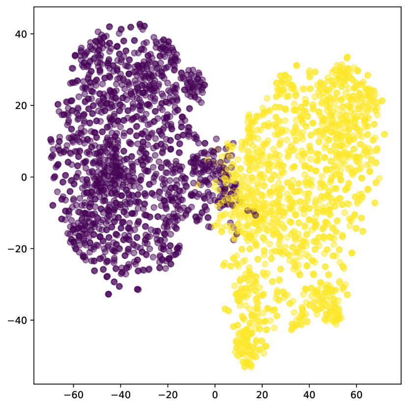
(b) Setting Minscale = $0.04$

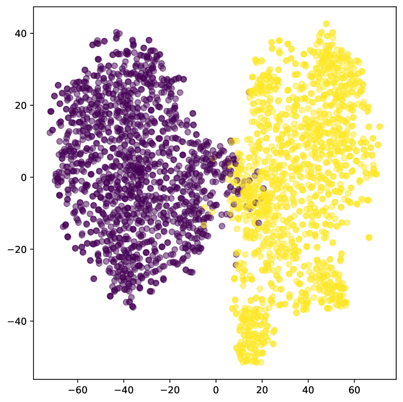
(c) Setting Minscale = $0.08$

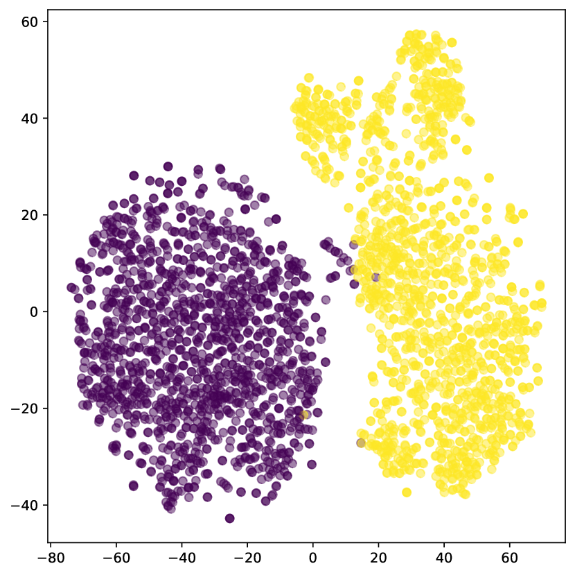
(d) Setting Minscale = $0.2$

(e) Setting Minscale = $0.5$

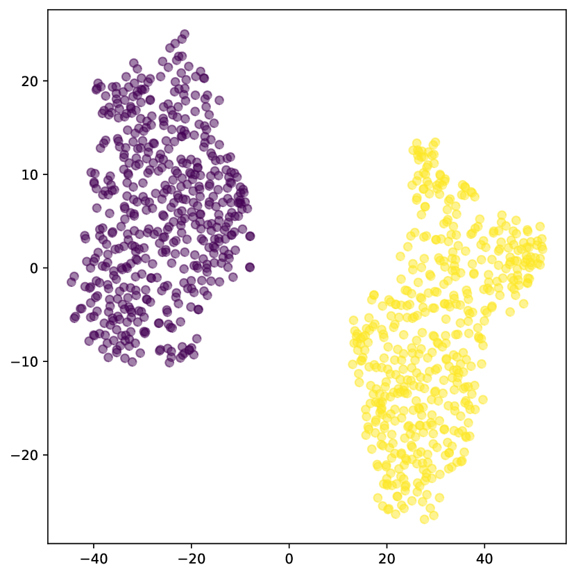
(f) Without using Augmentation

Figure 6: Visualization of samples with varying levels of data augmentation intensity. We visualize the samples of 2 classes from CIFAR-10 in 2-dimensional space, respectively setting minscale in RandomResizeCrop as $\{0.02,0.04,0.08,0.2,0.5\}$ and without data augmentation.

(a) Setting Minscale = $0.02$

(b) Setting Minscale = $0.04$

(c) Setting Minscale = $0.08$

(d) Setting Minscale = $0.2$

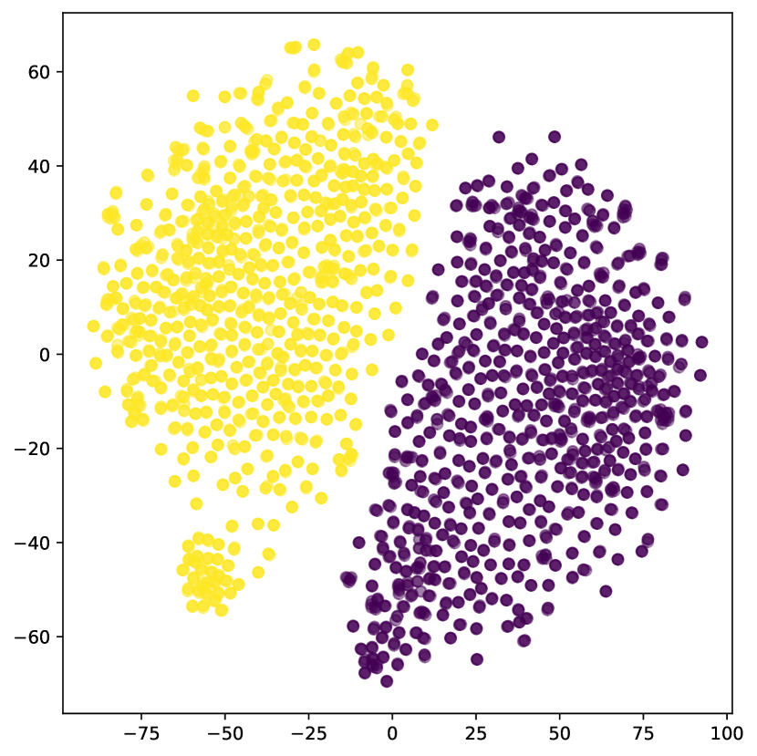
(e) Setting Minscale = $0.5$

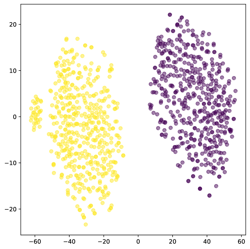
(f) Without using Augmentation

Figure 7: Visualization of samples with varying levels of data augmentation intensity. We visualize the samples of 2 classes from CIFAR-100 in 2-dimensional space, respectively setting minscale in RandomResizeCrop as $\{0.02,0.04,0.08,0.2,0.5\}$ and without data augmentation.

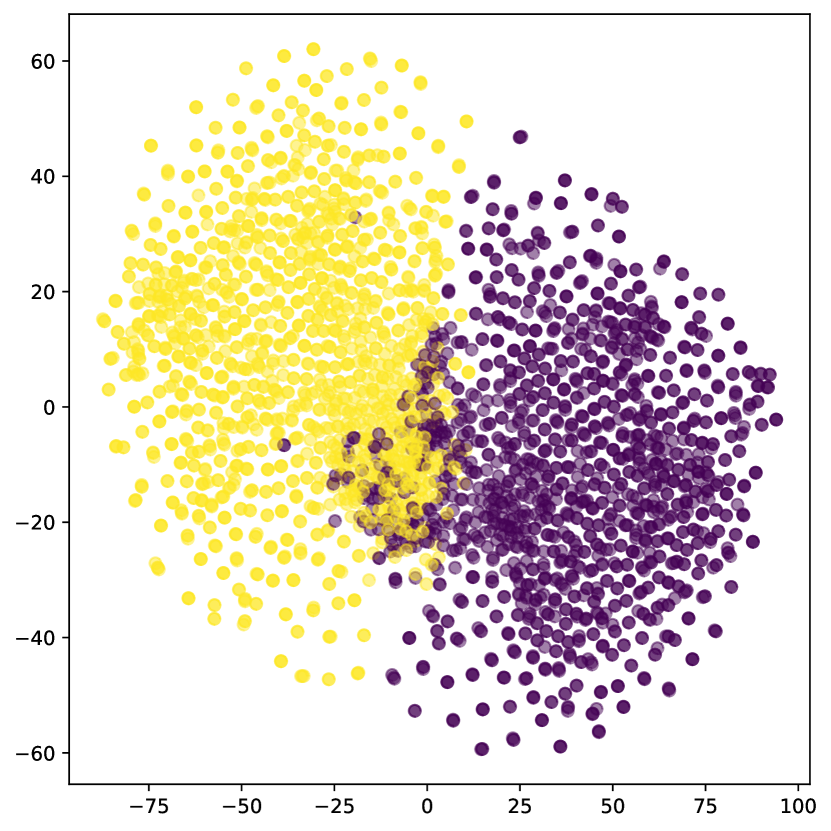
(a) Setting Minscale = $0.02$

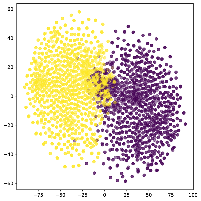
(b) Setting Minscale = $0.04$

(c) Setting Minscale = $0.08$

(d) Setting Minscale = $0.2$

(e) Setting Minscale = $0.5$

(f) Without using Augmentation

Figure 8: Visualization of samples with varying levels of data augmentation intensity. We visualize the samples of 2 classes from Tiny-ImageNet in 2-dimensional space, respectively setting minscale in RandomResizeCrop as $\{0.02,0.04,0.08,0.2,0.5\}$ and without data augmentation.

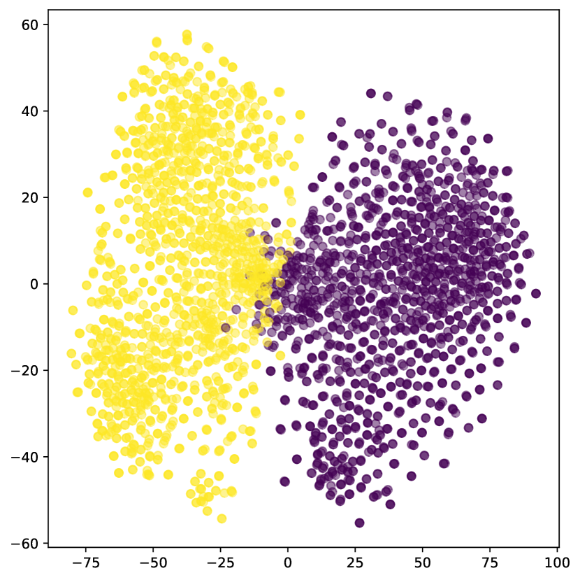
(a) Setting Minscale = $0.02$

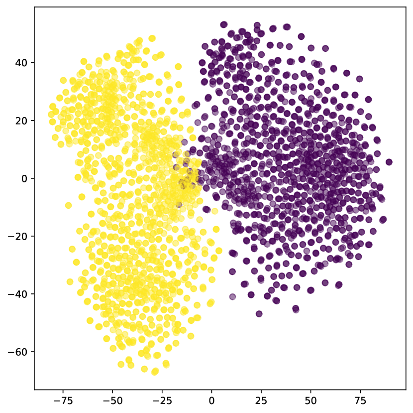
(b) Setting Minscale = $0.04$

(c) Setting Minscale = $0.08$

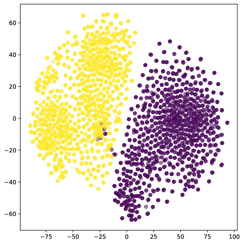
(d) Setting Minscale = $0.2$

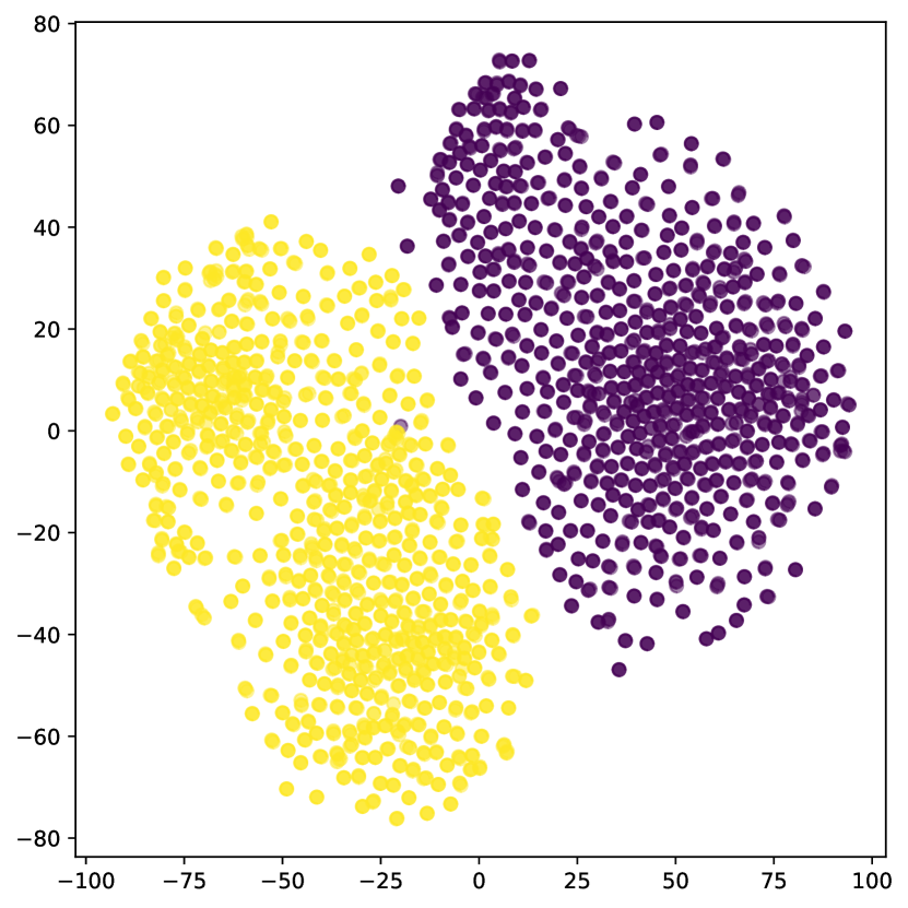
(e) Setting Minscale = $0.5$

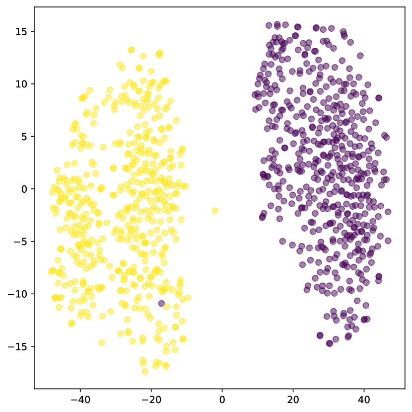
(f) Without using Augmentation

Figure 9: Visualization of samples with varying levels of data augmentation intensity. We visualize the samples of 2 classes from ImageNet-1K in 2-dimensional space, respectively setting minscale in RandomResizeCrop as $\{0.02,0.04,0.08,0.2,0.5\}$ and without data augmentation.

O.5 Empirical Analysis for Real-world Datasets

Beyond the theoretical analysis for a simple case, we also provide empirical analysis for four real-world datasets under different intensities of data augmentation. We utilize TSNE [60] to visualize the (augmented) samples in Figure 7; 7; 8; 9. All the results demonstrate that:

1. as minscale increases from 0.02 to 0.5, the data points gradually change from being tightly clustered to more dispersed. This indicates that higher data augmentation intensity expands the range of sample distribution;

2. when minscale=0.02, the data points of the two classes exhibit significant overlap, and the boundary becomes blurred. In contrast, larger minscale values such as 0.2 and 0.5 allow for better separation between classes;

3. when data augmentation is not used (the last figure), there is a clear gap between the two classes, and the data points within each class are very compact. This suggests that the feature distribution of the original samples is relatively concentrated.

References

- Achiam et al. [2023] Josh Achiam, Steven Adler, Sandhini Agarwal, Lama Ahmad, Ilge Akkaya, Florencia Leoni Aleman, Diogo Almeida, Janko Altenschmidt, Sam Altman, Shyamal Anadkat, et al. Gpt-4 technical report. arXiv preprint arXiv:2303.08774, 2023.
- Bai et al. [2023] Yutong Bai, Xinyang Geng, Karttikeya Mangalam, Amir Bar, Alan Yuille, Trevor Darrell, Jitendra Malik, and Alexei A Efros. Sequential modeling enables scalable learning for large vision models. arXiv preprint arXiv:2312.00785, 2023.
- Bardes et al. [2021] Adrien Bardes, Jean Ponce, and Yann LeCun. Vicreg: Variance-invariance-covariance regularization for self-supervised learning. arXiv preprint arXiv:2105.04906, 2021.
- Ben-David et al. [2010] Shai Ben-David, John Blitzer, Koby Crammer, Alex Kulesza, Fernando Pereira, and Jennifer Vaughan. A theory of learning from different domains. Machine Learning, 79:151–175, 2010. URL http://www.springerlink.com/content/q6qk230685577n52/.
- Bishop and Nasrabadi [2006] Christopher M Bishop and Nasser M Nasrabadi. Pattern recognition and machine learning, volume 4. Springer, 2006.
- Brown et al. [2020] Tom Brown, Benjamin Mann, Nick Ryder, Melanie Subbiah, Jared D Kaplan, Prafulla Dhariwal, Arvind Neelakantan, Pranav Shyam, Girish Sastry, Amanda Askell, et al. Language models are few-shot learners. Advances in neural information processing systems, 33:1877–1901, 2020.
- Burns et al. [2023] Collin Burns, Pavel Izmailov, Jan Hendrik Kirchner, Bowen Baker, Leo Gao, Leopold Aschenbrenner, Yining Chen, Adrien Ecoffet, Manas Joglekar, Jan Leike, et al. Weak-to-strong generalization: Eliciting strong capabilities with weak supervision. arXiv preprint arXiv:2312.09390, 2023.
- Cao et al. [2020] Yue Cao, Zhenda Xie, Bin Liu, Yutong Lin, Zheng Zhang, and Han Hu. Parametric instance classification for unsupervised visual feature learning. In NeurIPS, 2020.
- Caron et al. [2020] Mathilde Caron, Ishan Misra, Julien Mairal, Priya Goyal, Piotr Bojanowski, and Armand Joulin. Unsupervised learning of visual features by contrasting cluster assignments. In NeurIPS, 2020.
- Caron et al. [2021] Mathilde Caron, Hugo Touvron, Ishan Misra, Hervé Jégou, Julien Mairal, Piotr Bojanowski, and Armand Joulin. Emerging properties in self-supervised vision transformers. In ICCV, 2021.
- Cazenavette et al. [2022] George Cazenavette, Tongzhou Wang, Antonio Torralba, Alexei A Efros, and Jun-Yan Zhu. Dataset distillation by matching training trajectories. In Proceedings of the IEEE/CVF Conference on Computer Vision and Pattern Recognition, pages 4750–4759, 2022.
- Chen et al. [2020a] Ting Chen, Simon Kornblith, Mohammad Norouzi, and Geoffrey Hinton. A simple framework for contrastive learning of visual representations. In ICML, 2020a.
- Chen and He [2021] Xinlei Chen and Kaiming He. Exploring simple siamese representation learning. In CVPR, 2021.
- Chen et al. [2020b] Xinlei Chen, Haoqi Fan, Ross Girshick, and Kaiming He. Improved baselines with momentum contrastive learning. arXiv preprint arXiv:2003.04297, 2020b.
- Chen et al. [2021] Xinlei Chen, Saining Xie, and Kaiming He. An empirical study of training self-supervised vision transformers. arXiv preprint arXiv:2104.02057, 2021.
- Cheng et al. [2017] Yu Cheng, Duo Wang, Pan Zhou, and Tao Zhang. A survey of model compression and acceleration for deep neural networks. arXiv preprint arXiv:1710.09282, 2017.
- Cui et al. [2022] Justin Cui, Ruochen Wang, Si Si, and Cho-Jui Hsieh. Dc-bench: Dataset condensation benchmark. Advances in Neural Information Processing Systems, 35:810–822, 2022.
- Cui et al. [2023] Justin Cui, Ruochen Wang, Si Si, and Cho-Jui Hsieh. Scaling up dataset distillation to imagenet-1k with constant memory. In International Conference on Machine Learning, pages 6565–6590. PMLR, 2023.
- Da Costa et al. [2022] Victor Guilherme Turrisi Da Costa, Enrico Fini, Moin Nabi, Nicu Sebe, and Elisa Ricci. solo-learn: A library of self-supervised methods for visual representation learning. Journal of Machine Learning Research, 23(56):1–6, 2022.
- Deng et al. [2009] Jia Deng, Wei Dong, Richard Socher, Li-Jia Li, Kai Li, and Li Fei-Fei. Imagenet: A large-scale hierarchical image database. In 2009 IEEE conference on computer vision and pattern recognition, pages 248–255. Ieee, 2009.
- Dosovitskiy et al. [2020] Alexey Dosovitskiy, Lucas Beyer, Alexander Kolesnikov, Dirk Weissenborn, Xiaohua Zhai, Thomas Unterthiner, Mostafa Dehghani, Matthias Minderer, Georg Heigold, Sylvain Gelly, et al. An image is worth 16x16 words: Transformers for image recognition at scale. arXiv preprint arXiv:2010.11929, 2020.
- Du et al. [2023] Jiawei Du, Yidi Jiang, Vincent YF Tan, Joey Tianyi Zhou, and Haizhou Li. Minimizing the accumulated trajectory error to improve dataset distillation. In Proceedings of the IEEE/CVF Conference on Computer Vision and Pattern Recognition, pages 3749–3758, 2023.
- Goyal et al. [2019] Priya Goyal, Dhruv Mahajan, Abhinav Gupta, and Ishan Misra. Scaling and benchmarking self-supervised visual representation learning. In Proceedings of the ieee/cvf International Conference on computer vision, pages 6391–6400, 2019.
- Guo et al. [2023] Ziyao Guo, Kai Wang, George Cazenavette, Hui Li, Kaipeng Zhang, and Yang You. Towards lossless dataset distillation via difficulty-aligned trajectory matching. arXiv preprint arXiv:2310.05773, 2023.
- He et al. [2016] Kaiming He, Xiangyu Zhang, Shaoqing Ren, and Jian Sun. Deep residual learning for image recognition. In Proceedings of the IEEE conference on computer vision and pattern recognition, pages 770–778, 2016.
- He et al. [2020] Kaiming He, Haoqi Fan, Yuxin Wu, Saining Xie, and Ross Girshick. Momentum contrast for unsupervised visual representation learning. In CVPR, 2020.
- Hu et al. [2021] Qianjiang Hu, Xiao Wang, Wei Hu, and Guo-Jun Qi. Adco: Adversarial contrast for efficient learning of unsupervised representations from self-trained negative adversaries. In CVPR, 2021.
- Huang et al. [2019] Yanping Huang, Youlong Cheng, Ankur Bapna, Orhan Firat, Dehao Chen, Mia Chen, HyoukJoong Lee, Jiquan Ngiam, Quoc V Le, Yonghui Wu, et al. Gpipe: Efficient training of giant neural networks using pipeline parallelism. Advances in neural information processing systems, 32, 2019.
- Jean-Bastien et al. [2020] Grill Jean-Bastien, Strub Florian, Altché Florent, Tallec Corentin, Pierre Richemond H., Buchatskaya Elena, Doersch Carl, Bernardo Pires Avila, Zhaohan Guo Daniel, Mohammad Azar Gheshlaghi, Piot Bilal, Kavukcuoglu Koray, Munos Rémi, and Valko Michal. Bootstrap your own latent - a new approach to self-supervised learning. In NeurIPS, 2020.
- Kalantidis et al. [2020] Yannis Kalantidis, Mert Bulent Sariyildiz, Noe Pion, Philippe Weinzaepfel, and Diane Larlus. Hard negative mixing for contrastive learning. In NeurIPS, 2020.
- Kim et al. [2022] Jang-Hyun Kim, Jinuk Kim, Seong Joon Oh, Sangdoo Yun, Hwanjun Song, Joonhyun Jeong, Jung-Woo Ha, and Hyun Oh Song. Dataset condensation via efficient synthetic-data parameterization. In International Conference on Machine Learning, pages 11102–11118. PMLR, 2022.
- Kingma and Ba [2014] Diederik P Kingma and Jimmy Ba. Adam: A method for stochastic optimization. arXiv preprint arXiv:1412.6980, 2014.
- Krizhevsky et al. [2009a] Alex Krizhevsky, Geoffrey Hinton, et al. Learning multiple layers of features from tiny images. 2009a.
- Krizhevsky et al. [2009b] Alex Krizhevsky, Vinod Nair, and Geoffrey Hinton. Cifar-10 and cifar-100 datasets. URl: https://www. cs. toronto. edu/kriz/cifar. html, 6(1):1, 2009b.
- Le and Yang [2015] Ya Le and Xuan Yang. Tiny imagenet visual recognition challenge. CS 231N, 7(7):3, 2015.
- Lee et al. [2024] Dong Bok Lee, Seanie Lee, Joonho Ko, Kenji Kawaguchi, Juho Lee, and Sung Ju Hwang. Self-supervised dataset distillation for transfer learning. In Proceedings of the International Conference on Learning Representations (ICLR), 2024.
- Li et al. [2018] Hao Li, Zheng Xu, Gavin Taylor, Christoph Studer, and Tom Goldstein. Visualizing the loss landscape of neural nets. Advances in neural information processing systems, 31, 2018.
- Li et al. [2021] Junnan Li, Pan Zhou, Caiming Xiong, and Steven CH Hoi. Prototypical contrastive learning of unsupervised representations. In ICLR, 2021.
- Lin et al. [2018] Tao Lin, Sebastian U Stich, Kumar Kshitij Patel, and Martin Jaggi. Don’t use large mini-batches, use local sgd. arXiv preprint arXiv:1808.07217, 2018.
- Liu et al. [2023a] Xiao Liu, Yanan Zheng, Zhengxiao Du, Ming Ding, Yujie Qian, Zhilin Yang, and Jie Tang. Gpt understands, too. AI Open, 2023a.
- Liu et al. [2023b] Yanqing Liu, Jianyang Gu, Kai Wang, Zheng Zhu, Wei Jiang, and Yang You. Dream: Efficient dataset distillation by representative matching. arXiv preprint arXiv:2302.14416, 2023b.
- Mehta et al. [2024] Sachin Mehta, Maxwell Horton, Fartash Faghri, Mohammad Hossein Sekhavat, Mahyar Najibi, Mehrdad Farajtabar, Oncel Tuzel, and Mohammad Rastegari. Catlip: Clip-level visual recognition accuracy with 2.7 x faster pre-training on web-scale image-text data. arXiv preprint arXiv:2404.15653, 2024.
- Mohri et al. [2018] Mehryar Mohri, Afshin Rostamizadeh, and Ameet Talwalkar. Foundations of Machine Learning. 2018. URL https://mitpress.ublish.com/ebook/foundations-of-machine-learning--2-preview/7093/Cover. Second Edition.
- Oord et al. [2018] Aaron van den Oord, Yazhe Li, and Oriol Vinyals. Representation learning with contrastive predictive coding. arXiv preprint arXiv:1807.03748, 2018.
- Paszke et al. [2019] Adam Paszke, Sam Gross, Francisco Massa, Adam Lerer, James Bradbury, Gregory Chanan, Trevor Killeen, Zeming Lin, Natalia Gimelshein, Luca Antiga, et al. Pytorch: An imperative style, high-performance deep learning library. Advances in neural information processing systems, 32, 2019.
- Radford et al. [2021] Alec Radford, Jong Wook Kim, Chris Hallacy, Aditya Ramesh, Gabriel Goh, Sandhini Agarwal, Girish Sastry, Amanda Askell, Pamela Mishkin, Jack Clark, et al. Learning transferable visual models from natural language supervision. In International conference on machine learning, pages 8748–8763. PMLR, 2021.
- Richemond et al. [2020] Pierre H Richemond, Jean-Bastien Grill, Florent Altché, Corentin Tallec, Florian Strub, Andrew Brock, Samuel Smith, Soham De, Razvan Pascanu, Bilal Piot, et al. Byol works even without batch statistics. arXiv preprint arXiv:2010.10241, 2020.
- Robbins [1951] Herbert E. Robbins. A stochastic approximation method. Annals of Mathematical Statistics, 22:400–407, 1951. URL https://api.semanticscholar.org/CorpusID:16945044.
- Sandler et al. [2018] Mark Sandler, Andrew Howard, Menglong Zhu, Andrey Zhmoginov, and Liang-Chieh Chen. Mobilenetv2: Inverted residuals and linear bottlenecks. In Proceedings of the IEEE conference on computer vision and pattern recognition, pages 4510–4520, 2018.
- Shannon [1948] Claude Elwood Shannon. A mathematical theory of communication. The Bell system technical journal, 27(3):379–423, 1948.
- Shao et al. [2023] Shitong Shao, Zeyuan Yin, Muxin Zhou, Xindong Zhang, and Zhiqiang Shen. Generalized large-scale data condensation via various backbone and statistical matching. arXiv preprint arXiv:2311.17950, 2023.
- Shao et al. [2024] Shitong Shao, Zikai Zhou, Huanran Chen, and Zhiqiang Shen. Elucidating the design space of dataset condensation. arXiv preprint arXiv:2404.13733, 2024.
- Sorscher et al. [2022] Ben Sorscher, Robert Geirhos, Shashank Shekhar, Surya Ganguli, and Ari Morcos. Beyond neural scaling laws: beating power law scaling via data pruning. Advances in Neural Information Processing Systems, 35:19523–19536, 2022.
- Strubell et al. [2019] Emma Strubell, Ananya Ganesh, and Andrew McCallum. Energy and policy considerations for deep learning in nlp. arXiv preprint arXiv:1906.02243, 2019.
- Sun et al. [2024] Peng Sun, Bei Shi, Daiwei Yu, and Tao Lin. On the diversity and realism of distilled dataset: An efficient dataset distillation paradigm. In Proceedings of the IEEE/CVF Conference on Computer Vision and Pattern Recognition (CVPR), 2024.
- Susmelj et al. [2020] Igor Susmelj, Matthias Heller, Philipp Wirth, Jeremy Prescott, and Malte Ebner et al. Lightly. GitHub. Note: https://github.com/lightly-ai/lightly, 2020.
- Tan and Le [2019] Mingxing Tan and Quoc Le. Efficientnet: Rethinking model scaling for convolutional neural networks. In International conference on machine learning, pages 6105–6114. PMLR, 2019.
- Tao et al. [2022] Chenxin Tao, Honghui Wang, Xizhou Zhu, Jiahua Dong, Shiji Song, Gao Huang, and Jifeng Dai. Exploring the equivalence of siamese self-supervised learning via a unified gradient framework. In Proceedings of the IEEE/CVF Conference on Computer Vision and Pattern Recognition, pages 14431–14440, 2022.
- Tian et al. [2021] Yuandong Tian, Xinlei Chen, and Surya Ganguli. Understanding self-supervised learning dynamics without contrastive pairs. In ICML, 2021.
- Van der Maaten and Hinton [2008] Laurens Van der Maaten and Geoffrey Hinton. Visualizing data using t-sne. Journal of machine learning research, 9(11), 2008.
- Wang et al. [2021] Guangrun Wang, Keze Wang, Guangcong Wang, Philip HS Torr, and Liang Lin. Solving inefficiency of self-supervised representation learning. In Proceedings of the IEEE/CVF International Conference on Computer Vision, pages 9505–9515, 2021.
- Wang et al. [2022] Kai Wang, Bo Zhao, Xiangyu Peng, Zheng Zhu, Shuo Yang, Shuo Wang, Guan Huang, Hakan Bilen, Xinchao Wang, and Yang You. Cafe: Learning to condense dataset by aligning features. In Proceedings of the IEEE/CVF Conference on Computer Vision and Pattern Recognition, pages 12196–12205, 2022.
- Wang and Isola [2020] Tongzhou Wang and Phillip Isola. Understanding contrastive representation learning through alignment and uniformity on the hypersphere. In ICML, 2020.
- Wang et al. [2018] Tongzhou Wang, Jun-Yan Zhu, Antonio Torralba, and Alexei A Efros. Dataset distillation. arXiv preprint arXiv:1811.10959, 2018.
- Yin et al. [2023] Zeyuan Yin, Eric Xing, and Zhiqiang Shen. Squeeze, recover and relabel: Dataset condensation at imagenet scale from a new perspective. arXiv preprint arXiv:2306.13092, 2023.
- Yu et al. [2023] Ruonan Yu, Songhua Liu, and Xinchao Wang. Dataset distillation: A comprehensive review. arXiv preprint arXiv:2301.07014, 2023.
- Zbontar et al. [2021] Jure Zbontar, Li Jing, Ishan Misra, Yann LeCun, and Stéphane Deny. Barlow twins: Self-supervised learning via redundancy reduction. In ICML, 2021.
- Zhang et al. [2023] Lei Zhang, Jie Zhang, Bowen Lei, Subhabrata Mukherjee, Xiang Pan, Bo Zhao, Caiwen Ding, Yao Li, and Dongkuan Xu. Accelerating dataset distillation via model augmentation. In Proceedings of the IEEE/CVF Conference on Computer Vision and Pattern Recognition, pages 11950–11959, 2023.
- Zhao and Bilen [2023] Bo Zhao and Hakan Bilen. Dataset condensation with distribution matching. In Proceedings of the IEEE/CVF Winter Conference on Applications of Computer Vision, pages 6514–6523, 2023.
- Zhao et al. [2020] Bo Zhao, Konda Reddy Mopuri, and Hakan Bilen. Dataset condensation with gradient matching. arXiv preprint arXiv:2006.05929, 2020.
- Zhao et al. [2023] Ganlong Zhao, Guanbin Li, Yipeng Qin, and Yizhou Yu. Improved distribution matching for dataset condensation. In Proceedings of the IEEE/CVF Conference on Computer Vision and Pattern Recognition, pages 7856–7865, 2023.
- Zhu et al. [2021] Rui Zhu, Bingchen Zhao, Jingen Liu, Zhenglong Sun, and Chang Wen Chen. Improving contrastive learning by visualizing feature transformation. In ICCV, 2021.