Inflation in a scalar-vector gravity theory

Abstract

We study the possibility that inflation is driven by a scalar field together with a vector field minimally coupled to gravity. By assuming an effective potential that incorporates both fields into the action, we explore two distinct scenarios: one where the fields interact and another where they do not. In this context, we find different analytical solutions to the background scalar-vector fields dynamics during the inflationary scenario considering the slow-roll approximation. Besides, general conditions required for these models of two fields to be realizable are determined and discussed. From the cosmological perturbations, we consider a local field rotation, and then we determine these perturbations (scalar and tensor) during inflation, and we also utilize recent cosmological observations for constraining the parameter-space in these scalar-vector inflationary models.

1 Introduction

Inflation has emerged as a fundamental paradigm for describing the early universe’s physics. However, the identity of the field(s) responsible for driving inflation remains an open question. Future cosmological observations, particularly those related to the Cosmic Microwave Background (CMB), are hoped to help narrow down the possibilities and provide insights into the underlying physics.

The incorporation of scalar fields into the inflation framework is motivated by the quest for a dynamic driving force behind the accelerated expansion. The simplest inflationary scenario involves a canonical scalar field, denoted as $\phi$, which acts as the inflaton [1, 2, 3]. These scalar fields introduce a versatile energy component that can evolve over time. Its dynamical nature allows for variations in the equation of state during different epochs of inflation, offering a diverse landscape for exploring inflationary scenarios [4, 5, 6, 7, 8, 9]. This adaptability is crucial for constructing models that can be fine-tuned to match the increasingly precise observational data we gather from various cosmological surveys.

Notably, inflation based on scalar field offers a simple explanation for the origin of Cosmic Microwave Background (CMB) temperature anisotropies. Simultaneously, it provides a mechanism to account for the Large-Scale Structure (LSS) of our Universe by generating primordial density perturbations via quantum fluctuations during the inflationary epoch [10, 11, 12, 13]. These fluctuations are stretched to macroscopic scales by the rapid expansion, seeding the formation of galaxies and clusters observed today.

And, in the context of single-field inflation, curvature perturbation remains conserved on large scales. However, in multi-field inflation scenarios, the curvature perturbation can undergo significant modifications on large scales due to its sourcing from entropy (or isocurvature) perturbations. This intriguing feature was initially highlighted within the framework of Jordan-Brans-Dicke gravity, where the gravitational sector incorporates a scalar field [14]. This effect has further been illustrated within specific inflationary models based on string theory constructions [15, 16]. Consequently, adhering strictly to an effectively single-field scenario, despite its appealing simplicity, may sometimes lead to misleading conclusions. The final curvature perturbation, which will eventually be observed, can occasionally originate predominantly from the entropy modes. In the context of multi-field inflation, the intriguing possibility—depending on the reheating scenario—exists to generate both adiabatic and isocurvature perturbations after the inflationary phase. This correlation was pointed out in the literature [6, 7, 8].

On the other hand, the motivation to introduce vector fields within the cosmic inflation framework is rooted in the aspiration to broaden our theoretical perspective beyond scalar fields [17]. The inclusion of vector fields in inflationary models can lead to distinctive observational predictions that differ from those of scalar-driven inflation. These predictions may offer valuable insights into the underlying physics of the inflationary epoch and provide a means of discriminating between different inflationary scenarios [18].

Vector fields offer solutions to some of the shortcomings or unanswered questions in traditional scalar-driven inflationary models. They have the potential to address issues such as the generation of primordial magnetic fields, the origin of large-scale structures, and the generation of anisotropies in the cosmic microwave background radiation [18]. By exploring the dynamics and implications of vector fields in cosmic inflation, we can advance our understanding of the early universe. Investigating the role of vector fields in driving inflationary expansion allows us to gain deeper insights into the fundamental processes that shaped the cosmos during its formative stages [19].

The coupling between scalar and vector fields introduces distinctive observational consequences that serve as probes for validating or constraining inflationary models. Constraints derived from cosmic microwave background (CMB) observations, such as those obtained by the Planck satellite mission [20, 21], play a crucial role in delineating the parameter space of scalar-vector coupling scenarios. Additionally, analyses of large-scale structure surveys, such as the Sloan Digital Sky Survey (SDSS) [22, 23], offer complementary insights into the impact of scalar-vector interactions on the clustering properties of galaxies and dark matter halos.

Moreover, gravitational wave experiments, such as those conducted by the Laser Interferometer Gravitational-Wave Observatory (LIGO) [24, 25], provide unique opportunities to probe the cosmic fabric for signatures of primordial gravitational waves generated during inflation. Scalar-vector coupling dynamics can leave distinct imprints on the stochastic gravitational wave background, offering a tantalizing prospect for direct observational validation of inflationary scenarios featuring coupled fields.

Extensions of the standard inflationary paradigm, such as multi-field inflation models [6, 7, 8], motivate to incorporate scalar-vector interactions to explore the rich phenomenology of early-universe dynamics. By incorporating both scalar and vector degrees of freedom, these frameworks offer novel avenues for addressing fundamental questions regarding the origin of cosmic structure and the nature of dark energy.

Furthermore, cosmological simulations utilizing state-of-the-art computational techniques [26] enable detailed investigations into the formation and evolution of cosmic structures within scalar-vector coupled inflationary scenarios. These simulations provide invaluable insights into the nonlinear dynamics of cosmic strings, their gravitational effects, and their observational implications, fostering a deeper understanding of the cosmic ballet orchestrated by scalar and vector fields during the inflationary epoch.

In summary, the exploration of scalar-vector coupling within the inflationary paradigm represents a frontier in theoretical cosmology, offering a fertile ground for interdisciplinary research at the interface of particle physics, astrophysics, and cosmology. As observational data improves in quality and quantity, ongoing efforts to refine and confront scalar-vector coupled inflationary models with empirical evidence will undoubtedly enrich our understanding of the early universe and its intricate tapestry of fundamental interactions.

The outline of the paper is as follows: The next section shows the background dynamics considering the slow roll approximation in a scalar-vector gravity theory. In section 3, we analyze the cosmological perturbations for double inflation, and we obtain explicit expressions for the scalar power spectrum, spectral index, and tensor-to-scalar ratio under a local field rotation. In section 4, we study the first example of our model, in which we consider a specific potential in which there is no interaction between the fields. In section 5, we analyze a second example, in which we study an effective potential that presents an interaction between the scalar field and the vector field. Finally, section 6 resumes our results and exhibits our conclusions. We chose units so that $c=\hbar=1$.

2 Scalar Vector gravity theory

We start with the action for the Maxwell scalar gravity theory given by[27, 28]

$$S=\int{d^{4}x\sqrt{-g}\left[-\frac{R}{2\kappa^{2}}+f(\phi,X_{1},X_{3})\right]},$$ (1)

where $R$ is the Ricci scalar curvature, $\kappa^{2}=8\pi G=8\pi/M_{Pl}^{2}$, $g$ denotes to the determinant of the metric tensor $g_{\mu\nu}$. Besides, the function $f(\phi,X_{1},X_{3})$ corresponds to an arbitrary function associated to the scalar field $\phi$ along with its kinetic term $X_{1}$ and the mass term related to the vector field $X_{3}$, with which we have

$$X_{1}=-\dfrac{1}{2}\nabla_{\mu}\phi\nabla^{\mu}\phi,\ \ \ \ X_{3}=-\dfrac{1}{2}A_{\mu}A^{\mu},$$ (2)

where $A^{\mu}$ is four vector potential with norm $A^{2}=g_{\mu\nu}A^{\mu}A^{\nu}$. In the following and in order to define the arbitrary function $f(\phi,X_{1},X_{3})$, we will consider the function

$$f(\phi,X_{1},X_{3})=X_{1}-\frac{1}{4}F_{\mu\nu}F^{\mu\nu}-V(\phi,X_{3}),$$ (3)

where the antisymmetric field strength tensor $F_{\mu\nu}$ is defined as $F_{\mu\nu}=\partial_{\mu}A_{\nu}-\partial_{\nu}A_{\mu}$ and $V(\phi,X_{3})$ corresponds to an effective potential associated to the scalar field $\phi$ and the vector field $X_{3}$.

By assuming that the vector field is a purely time-like vector in which $A^{\mu}=(A,A^{i})=(A(t),0)=(A,0)$ (with $i=1,2,3$) together with a homogeneous scalar field $\phi=\phi(t)$ and considering a spatially flat Friedmann Robertson Walker metric, we obtain that the background equations result

$$\frac{3H^{2}}{\kappa^{2}} = \frac{3}{2}(AH+\dot{A})^{2}+\dfrac{1}{2}\dot{\phi}^{2}+V,$$ (4)

$$-\frac{2\dot{H}}{\kappa^{2}} = -A^{2}V_{,X_{3}}+2(AH+\dot{A})^{2}+\dot{\phi}^{2},$$ (5)

$$\ddot{\phi}+3H\dot{\phi}+V_{,\phi}=0,$$ (6)

and

$$\dfrac{d(AH+\dot{A})}{dt}+2H(AH+\dot{A})=AV_{,X_{3}},$$ (7)

here, we have considered that $X_{3}=A^{2}/2$. Besides, the quantity $H=\dot{a}/a$ corresponds to the Hubble parameter, where $a$ denotes the scale factor.

In the following, we will utilize that the dots correspond differentiation with respect to the time, and we will use that the notation $V(\phi,X_{3})=V$, $V_{,\phi}$ represents $V_{,\phi}=\partial V/\partial\phi$, $V_{,X_{3}}$ to $V_{,X_{3}}=\partial V/\partial X_{3}$, etc.

In order to study the inflationary scenario, it is useful to introduce the following slow-roll parameters:

$$\epsilon_{\phi}=\dfrac{1}{2\kappa^{2}}\left(\dfrac{V_{,\phi}}{V}\right)^{2},\ \ \ \ \ \ \ \ \epsilon_{A}=\dfrac{1}{2\kappa^{2}}\left(\dfrac{AV_{,X_{3}}}{V}\right)^{2},$$ (8)

$$\eta_{\phi\phi}=\dfrac{1}{\kappa^{2}}\left(\dfrac{V_{,\phi\phi}}{V}\right),\ \ \ \ \ \ \ \ \eta_{\phi A}=\dfrac{1}{\kappa^{2}}\left(\dfrac{AV_{,\phi X_{3}}}{V}\right),\,\,\,\,\,\mbox{and}\ \ \ \ \ \ \ \ \eta_{AA}=\dfrac{1}{\kappa^{2}}\left(\dfrac{A^{2}V_{,X_{3}X_{3}}}{V}\right),$$ (9)

respectively. Thus, under the slow-roll approximation, these parameters are much less than the unit, and then the background equations are reduced to

$$\frac{3H^{2}}{\kappa^{2}} \simeq V,$$ (10)

$$3H\dot{\phi} \simeq -V_{,\phi},$$ (11)

$$2H(AH+\dot{A}) \simeq AV_{,X_{3}}.$$ (12)

Also, we note that the Eqs.(11) and (12) can be rewritten in terms of the slow roll parameters as

$$\dot{\phi}^{2}\simeq\dfrac{2}{3}\epsilon_{\phi}V,\,\,\,\,\,\,\mbox{and}\ \ \ \ \ \ \ \ (AH+\dot{A})^{2}\simeq\dfrac{3}{2}\epsilon_{A}V,$$ (13)

respectively.

Additionally, from equation (5) and considering that the parameter $\epsilon=-\dot{H}/H^{2}$, we can write

$$\epsilon\simeq-\dfrac{3}{\sqrt{2}}A\kappa\sqrt{\epsilon_{A}}+\dfrac{9}{2}\epsilon_{A}+\epsilon_{\phi}.$$ (14)

By combining the equations under the slow roll approximation (10)-(12), we can find a relation between the scalar field $\phi$ and the scalar $A$ associated to the vector field given by

$$\dfrac{d\phi}{d\ln A}\simeq-\dfrac{2}{3}\left(\dfrac{V_{,\phi}}{V_{,X_{3}}-\frac{2}{3}\kappa^{2}V}\right).$$ (15)

In this way, depending on the chosen effective potential $V=V(\phi,X_{3})=V(\phi,A^{2}/2)$, we could obtain an analytical solution to Eq.(15) and then we could find the relation $\phi=\phi(A)$ or vice versa, i.e., $A=A(\phi)$.

3 Cosmological Perturbations

In this section, we will analyze the cosmological perturbations in our model. Following Refs.[29, 30], we have that the perturbed Klein-Gordon equations by considering a perturbed FRW metric spacetime become

$$\delta\ddot{\phi}+3H\delta\dot{\phi}+\left[\dfrac{k^{2}}{a^{2}}+V_{\phi\phi}-\dfrac{\kappa^{2}}{a^{3}}\dfrac{d}{dt}\left(\dfrac{a^{3}}{H}\dot{\phi}^{2}\right)\right]\delta\phi$$

$$=\left[AV_{,\phi X3}+3\dfrac{\kappa^{2}}{a^{3}}\dfrac{d}{dt}\left(\dfrac{a^{3}}{H}\dot{\phi}(AH+\dot{A})\right)\right]\delta A,$$ (16)

and

$$3\delta\ddot{A}+9H\delta\dot{A}+\left[\dfrac{k^{2}}{a^{2}}+A^{2}V_{,X3X3}-3\dfrac{\kappa^{2}}{a^{3}}\dfrac{d}{dt}\left(\dfrac{a^{3}}{H}(AH+\dot{A})^{2}\right)\right]\delta A$$

$$=\left[AV_{,\phi X3}+3\dfrac{\kappa^{2}}{a^{3}}\dfrac{d}{dt}\left(\dfrac{a^{3}}{H}\dot{\phi}(AH+\dot{A})\right)\right]\delta\phi,$$ (17)

respectively.

By considering the linear perturbation on large scales in which $k\gg aH$ and neglecting those terms which include second order time derivatives and using the slow roll parameters given by Eqs.(8) and (9), we find that the perturbed Klein-Gordon equations can be approximate to

$$H^{-1}\delta\dot{\phi}+\left[\eta_{\phi\phi}-2\epsilon_{\phi}\right]\delta\phi\simeq\left[\eta_{\phi A}\pm 9\sqrt{\epsilon_{\phi}\epsilon_{A}}\right]\delta A,$$ (18)

and

$$3H^{-1}\delta\dot{A}+\left[\eta_{AA}-\dfrac{27}{2}\epsilon_{A}\right]\delta A\simeq\left[\eta_{\phi A}\pm 9\sqrt{\epsilon_{\phi}\epsilon_{A}}\right]\delta\phi.$$ (19)

For the case of the scalar perturbations in a system with two fields (double inflation) and following Refs.[30, 31], we must utilize a local field rotation in order to recognize the adiabatic and entropy perturbations in the orthogonal form to the background trajectory in field space. Thus, considering this rotation on the perturbed quantities, we can define two quantities $\delta\sigma$ and $\delta s$, in which $\sigma$ represents the “adiabatic field” and $s$ denotes the “entropy field” such that[31]

$$\delta\sigma=\cos{\theta}\delta\phi+\sin{\theta}\delta A,\,\,\,\,\,\,\,\,\,\mbox{and}\,\,\,\,\,\,\,\,\delta s=-\sin{\theta}\delta\phi+\cos{\theta}\delta A,$$ (20)

where the angle $\theta$ is related to the slow roll parameters from the relation $\tan\theta=(AH+\dot{A})/\dot{\phi}=a^{-1}(aA\dot{)}/\dot{\phi}=(3/2)\sqrt{\epsilon_{A}/\epsilon_{\phi}}$. Under this rotation, the curvature and entropy perturbations during the inflationary epoch can be written in standard form as; $\mathcal{R}\simeq\dfrac{H\delta\sigma}{\dot{\sigma}}\mbox{and}\,\,\mathcal{S}\simeq\dfrac{H\delta s}{\dot{\sigma}}$, respectively[30, 31].

From this rotation, we have that the slow-roll parameter associated to the slope orthogonal to the trajectory, $\epsilon_{s}\simeq 0$, and the new slow-roll parameters related to $\sigma$ and $s$ fields can be written as [30]

$$\eta_{\sigma s} = \frac{1}{3}\eta_{\text{AA}}\sin^{2}(\theta)-\frac{4}{3}\eta_{\text{$\phi$A}}\sin(\theta)\cos(\theta)+\eta_{\phi\phi}\cos^{2}(\theta),$$ (21)

$$\eta_{\sigma\sigma} = \frac{1}{3}\eta_{\text{AA}}\sin(\theta)\cos(\theta)+\frac{1}{3}\eta_{\text{$\phi$A}}\sin^{2}(\theta)-\eta_{\text{$\phi$A}}\cos^{2}(\theta)-\eta_{\phi\phi}\sin(\theta)\cos(\theta),$$ (22)

$$\eta_{ss} = \frac{1}{3}\eta_{\text{AA}}\cos^{2}(\theta)+\frac{4}{3}\eta_{\text{$\phi$A}}\sin(\theta)\cos(\theta)+\eta_{\phi\phi}\sin^{2}(\theta),$$ (23)

and the parameter associated to the slope of $V_{,\sigma}$ is defined as

$$\epsilon=\dfrac{1}{2\kappa^{2}}\left(\dfrac{V_{,\sigma}}{V}\right)^{2}\simeq-\dfrac{3}{\sqrt{2}}A\kappa\sqrt{\epsilon_{A}}+\dfrac{9}{2}\epsilon_{A}+\epsilon_{\phi}.$$ (24)

Besides, from this rotation, the background equations can be rewritten as

$$\dot{\sigma}^{2}\simeq\dfrac{2}{3}\epsilon\,V,\ \ \ \ \ \ \ H^{-1}\dot{\theta}\simeq-\eta_{\sigma s},$$ (25)

and the adiabatic and entropy perturbations satisfy the following equations:

$$H^{-1}\delta\dot{\sigma} \simeq (2\epsilon-\eta_{\sigma\sigma})\delta\sigma-2\eta_{\sigma s}\delta s,$$ (26)

$$H^{-1}\delta\dot{s} \simeq -\eta_{ss}\delta s.$$ (27)

In this form, following Refs.[30, 31], the adiabatic and entropy power spectrum at Hubble-crossing when $k=a_{*}H_{*}$ can be defined as

$$\mathcal{P}_{\mathcal{R}}|_{*}\simeq\mathcal{P}_{\mathcal{S}}|_{*}\simeq\left(\frac{H^{2}}{2\pi\dot{\sigma}}\right)_{*}^{2}\simeq\dfrac{8}{3\epsilon}\kappa^{4}V_{*}.$$ (28)

In what follows, the subscript $*$ is utilized to denote the epoch in which the cosmological scale exits the horizon.

Also, the scalar spectral index $n_{\mathcal{R}}$ associated to the adiabatic perturbation together with the scalar spectral index $n_{\mathcal{S}}$ related to the entropy spectrum at the Hubble crossing become [30]

$$n_{\mathcal{R}}|_{*}\simeq n_{\mathcal{S}}|_{*}\simeq-6\epsilon_{*}+2\eta_{{\sigma\sigma}_{*}}.$$ (29)

Here the scalar spectral index $n_{\mathcal{R}}$ and $n_{\mathcal{S}}$ are defined as $n_{\mathcal{R}}=d\ln\mathcal{P}_{\mathcal{R}}/d\ln k$ and $n_{\mathcal{S}}=d\ln\mathcal{P}_{\mathcal{S}}/d\ln k$, respectively.

In relation to the generation of tensor perturbation $\mathcal{P}_{T}$ during the inflationary scenario, it remains unaltered in the framework of double inflation and then under the slow-roll approximation yields [32, 33]

$$\mathcal{P}_{T}|_{*}\simeq\dfrac{128}{3}\kappa^{4}V_{*}\,.$$ (30)

The tensor spectral index $n_{T}$ associated to the tensor perturbation is expressed in terms of the slow-roll parameter $\epsilon$ as $n_{T}|_{*}=d\ln\mathcal{P}_{T}/d\ln k|_{*}=-2\,\epsilon$.

Additionally, an important observational quantity corresponds to the tensor-to-scalar ratio, denoted as $r$. This observational parameter at Hubble-crossing can be written as

$$r|_{*}=\left(\dfrac{\mathcal{P}_{T}}{\mathcal{P}_{\mathcal{R}}}\right)_{*}\simeq 16\epsilon|_{*}\simeq-8n_{T}|_{*}.$$ (31)

In the following, we will explore some inflationary stages within the framework of a scalar vector gravity theory. Specifically, we will investigate the inflationary scenario, assuming two types of effective potentials, $V(\phi,X_{3})$, associated with double inflation. Firstly, we will analyze a separable potential of the form $V(\phi,X_{3})=\bar{V}(\phi)+\tilde{V}(X_{3})$, in order to describe an inflationary stage, where there is no interaction between the fields $\phi$ and $X_{3}$. In a second scenario, we will analyze a potential $V$, in which the fields interact by mean of the product of the potentials $\bar{V}(\phi)$ and $\tilde{V}(X_{3})$, such that the effective potential $V(\phi,X_{3})$ is defined as $V(\phi,X_{3})=\bar{V}(\phi)\times\tilde{V}(X_{3})$.

4 Example I: Effective Potential $V(\phi,X_{3})=\bar{V}(\phi)+\tilde{V}(X_{3})$

In this section, we will assume a specific potential in which there is no interaction between the fields. The effective potential (separable potential) can be expressed as the sum of $\bar{V}(\phi)$ and $\tilde{V}(X_{3})$ such that [34, 35]

$$V(\phi,X_{3})=\bar{V}(\phi)+\tilde{V}(X_{3}),$$ (32)

where $\bar{V}(\phi)$ and $\tilde{V}(X_{3})$ are two arbitrary potentials that exclusively depend on the scalar field $\phi$ and $X_{3}$, respectively. From Eq.(15), we find that the relation between both fields can be determined from the equation

$$\dfrac{d\phi}{d\ln X_{3}}=-\dfrac{1}{3}\left(\dfrac{\bar{V}_{,\phi}}{\tilde{V}_{,X_{3}}-\frac{2}{3}\kappa^{2}\tilde{V}-\frac{2}{3}\kappa^{2}\bar{V}}\right),$$ (33)

and the number of e-folds $N$ defined as $dN=Hdt$ results

$$dN=-\kappa^{2}\dfrac{\bar{V}}{\bar{V}_{,\phi}}d\phi+\dfrac{\kappa^{2}}{3X_{3}}\dfrac{\tilde{V}}{(\tilde{V}_{,X_{3}}-\frac{2}{3}\kappa^{2}\tilde{V}-\frac{2}{3}\kappa^{2}\bar{V})}dX_{3}.$$ (34)

In order to derive an analytical expressions for this separable potential, we can consider that the effective potentials for $\bar{V}(\phi)$ and $\tilde{V}(X_{3})$ are exponential potentials defined as

$$\bar{V}(\phi)=\bar{V}_{0}e^{\alpha_{1}\phi^{2}},\,\,\,\,\,\,\mbox{and}\,\,\,\,\,\,\tilde{V}(X_{3})=\tilde{V}_{0}e^{\alpha_{2}\,X_{3}},$$ (35)

respectively. Here $\bar{V}_{0}$ and $\tilde{V}_{0}$ are two arbitrary constants, representing the amplitude of their respective potentials, and $\alpha_{1}$ and $\alpha_{2}$ correspond to two constants with dimensions of $\kappa^{2}$ (or $M_{Pl}^{-2}$). The exponential potentials in the context of the early universe have been extensively investigated in the literature, see e.g., Refs.[36, 37]

In order to find an analytical relation between the fields $\phi$ and $X_{3}$, we consider the special case in which the constant $\alpha_{1}=(3/4)\alpha_{2}=\kappa^{2}/2$. Thus, combining Eqs.(33) and (35), we find that the relation between the fields $\phi$ and $X_{3}$ is given by

$$\dfrac{d\phi}{dX_{3}}=\dfrac{\phi}{2X_{3}}\,\,\,\,\,\,\,\Rightarrow\,\,\,\,\,\,\,\,\,\,\,X_{3}=X_{3}^{(0)}\phi^{2},$$ (36)

where $X_{3}^{(0)}$ corresponds to a new integration constant (dimensionless).

Introducing the number of e-folds $N$ between two values of times $t_{*}$ and $t_{f}$ (or between two values of the scalar fields) we have

$$N=\int_{t_{*}}^{t_{f}}Hdt\simeq\int_{\phi_{f}}^{\phi_{*}}\dfrac{1}{\phi}d\phi-\dfrac{1}{2}\dfrac{\tilde{V}_{0}}{\bar{V}_{0}}\int_{X_{3f}}^{X_{3*}}\dfrac{1}{X_{3}}\dfrac{e^{\frac{2}{3}\kappa^{2}X_{3}}}{e^{\frac{\kappa^{2}\phi^{2}}{2}}}dX_{3},$$ (37)

where $t_{*}$ corresponds to the time when the cosmological scale exits the horizon, and the time $t_{f}$ denotes the end of the inflationary epoch.

In this way, from Eq.(37) we obtain that the number of $e-$folds N can be written as

$$N=\ln\left(\frac{\phi_{*}}{\phi_{f}}\right)-\left(\frac{1}{2}\frac{\tilde{V}_{0}}{\bar{V}_{0}}\right)\,(\mbox{Ei}[b_{1}X_{3_{*}}]-\mbox{Ei}[b_{1}X_{3_{f}}]),$$ (38)

where the constant $b_{1}=\kappa^{2}[2/3-(2X_{3}^{(0)})^{-1}]$ and the function Ei[z] corresponds to the exponential integral, see Ref.[38].

In order to find an analytical expression for the scalar field $\phi$ (or $X_{3}$) when the cosmological scale exists the horizon, we can assume small values of $X_{3}$ during the inflationary scenario. In this way, considering the relation between $\phi$ and $X_{3}$ given by Eq.(36), we obtain that the number of $e-$ folds from Eq.(38) is simplified to

$$N\simeq\ln{\left(\dfrac{\phi_{*}^{\frac{\tilde{V}_{0}}{\bar{V}_{0}}+1}}{\phi_{f}^{\frac{\tilde{V}_{0}}{\bar{V}_{0}}+1}}\right)},$$ (39)

and then the scalar field $\phi$ when the cosmological scale exits the horizon yields

$$\phi_{*}\simeq\phi_{f}e^{\dfrac{N}{\frac{\tilde{V}_{0}}{\bar{V}_{0}}+1}}.$$ (40)

Also, in order to find the scalar field at the end of inflation, we can consider that inflation ends when the slow roll parameter $\epsilon=1$ (or equivalently $\ddot{a}=0$). Thus, from Eq.(14) we obtain that the scalar field at the end of the inflationary epoch $\phi_{f}$ results

$$\phi_{f}\simeq\frac{\sqrt{2}(\bar{V}_{0}+\tilde{V}_{0})}{\kappa\sqrt{\bar{V}_{0}}\sqrt{\bar{V}_{0}-4\tilde{V}_{0}X_{3}^{(0)}}},$$ (41)

where the amplitude $\bar{V}_{0}>4\tilde{V}_{0}\,X_{3}^{(0)}$, in order to obtain a real value for the scalar field at the end of inflation. In particular, if the potential $\bar{V}_{0}\gg\tilde{V}_{0}\,X_{3}^{(0}$ then the scalar field at the end of inflation is simplified to $\phi_{f}\simeq[1+\tilde{V}_{0}/\bar{V}_{0}](\sqrt{2}/\kappa)$.

On the other hand, in relation to the cosmological perturbations, we find that the scalar power spectrum when the cosmological scale exits the horizon for these exponential potentials becomes

$$\mathcal{P}_{\mathcal{R}}|_{*}=\mathcal{P}_{\mathcal{R}_{*}}\simeq\frac{16\kappa^{2}(\bar{V}_{0}+\tilde{V}_{0})^{3}}{3\bar{V}_{0}\phi_{*}^{2}(\bar{V}_{0}-4\tilde{V}_{0}X_{3}^{(0)})}=\dfrac{8}{3}\kappa^{4}(\bar{V}_{0}+\tilde{V}_{0})e^{-\frac{2N_{*}}{\frac{\tilde{V}_{0}}{\bar{V}_{0}}+1}}.$$ (42)

Here we have utilized Eqs.(28), (36), (40) and (41), respectively.

Additionally, from Eq.(29) the scalar spectral index can be written in terms of the number of $e-$ folds $N$ as

$$n_{\mathcal{R}}|_{*}\simeq-\frac{\kappa^{2}\phi_{*}^{2}\left(27\bar{V}_{0}^{2}-124\bar{V}_{0}\tilde{V}_{0}X_{3}^{(0)}-16\tilde{V}_{0}^{2}X_{3}^{(0)}\right)}{9(\bar{V}_{0}+\tilde{V}_{0})^{2}}$$

$$=-\frac{2e^{\frac{2N_{*}}{\frac{\tilde{V}_{0}}{\bar{V}_{0}}+1}}\left(27\bar{V}_{0}^{2}-124\bar{V}_{0}\tilde{V}_{0}X_{3}^{(0)}-16\tilde{V}_{0}^{2}X_{3}^{(0)}\right)}{9\bar{V}_{0}(\bar{V}_{0}-3\tilde{V}_{0})}.$$ (43)

Here, we have used that

$$\cos\theta=\frac{\sqrt{4\epsilon_{\phi}}}{\sqrt{9\epsilon_{A}+4\epsilon_{\phi}}},\,\,\,\,\mbox{and}\,\,\,\,\sin\theta=\frac{\sqrt{9\epsilon_{A}}}{\sqrt{9\epsilon_{A}+4\epsilon_{\phi}}},$$

to determine the slow roll parameter $\eta_{\sigma\sigma}$ associated to the scalar spectral index $n_{\mathcal{R}}$, see Eq.(29).

Besides, the tensor-scalar ratio at Hubble-crossing as a function of the number of $e-$folds $N$ results

$$r|_{*}=r_{*}\simeq\frac{8\kappa^{2}\bar{V}_{0}\phi_{*}^{2}(\bar{V}_{0}-4\tilde{V}_{0}X_{3}^{(0)})}{(\bar{V}_{0}+\tilde{V}_{0})^{2}}=16e^{\frac{2N_{*}}{\frac{\tilde{V}_{0}}{\bar{V}_{0}}+1}}\,,$$ (44)

where we have used Eq.(31).

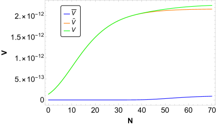
Figure 1: Evolution of the potentials $\overline{V}$ and $\tilde{V}$ and the total potential $V=\overline{V}+\tilde{V}$ in terms of the number of $e-$ folds $N$ during the inflationary epoch. Here, we have utilized the constraints on the parameters given by Eq.(45).

In order to find the parameters $\bar{V}_{0}$, $\tilde{V}_{0}$ and $X_{3}^{(0)}$, we can consider that the observational parameters take the following values; the power spectrum $\mathcal{P}_{\mathcal{R}_{*}}=2.2*10^{-9}$, $n_{\mathcal{R}_{*}}=0.967$ and the tensor scalar ratio $r_{*}=0.04$ at the number of $e-$ folds $N_{*}=60$. In this form, we obtain the following constraints on the parameter space:

$$\bar{V}_{0}\simeq 1.03\times 10^{-13}\kappa^{-4},\,\,\,\,\,\tilde{V}_{0}\simeq 2.17\times 10^{-12}\kappa^{-4},\,\,\,\mbox{and}\,\,\,\,\,X_{3}^{(0)}\simeq-1.21\times 10^{-2},$$ (45)

respectively. Here we have utilized Eqs.(42), (43) and (44).

In Fig.(1) we show the evolution of the potentials $\bar{V}(\phi)$, $\tilde{V}(X_{3})$ and the total potential $V(\phi,X_{3})$ as a function of the number of $e-$folds $N$. Here, we have considered the constraints on the space-parameter given by Eq.(45), which were obtained using the observational Planck data[20]. In order to write down values of the effective potentials $\bar{V}(\phi)$, $\tilde{V}(X_{3})$ and the total potential $V(\phi,X_{3})$ as a function of the number of $e-$folds $N$, we have used Eqs.(35), (36) and (40). Thus, from this plot, we can note that $\tilde{V}(X_{3})>\bar{V}(\phi)$ due to the constraints found on the parameter-space given by Eq.(45). In this way, we can conclude that the inflationary expansion of the universe is driven by the field $X_{3}$ from its potential $V(X_{3})$, since during inflation $3H^{2}\simeq\kappa^{2}\,V\sim\kappa^{2}\tilde{V}(X_{3})$.

5 Example II: Effective Potential $V(\phi,X_{3})=\bar{V}(\phi)\,\times\tilde{V}(X_{3})$

In this section, we will analyze an effective potential involving an interaction between the fields $\phi$ and $X_{3}$. This interaction is represented by the product of their individual potentials, $\bar{V}(\phi)$ and $\tilde{V}(X_{3})$. In this context, we consider, as a second example, the effective potential $V(\phi,X_{3})$ given by [39]

$$V(\phi,X_{3})=V=\bar{V}(\phi)\,\times\,\tilde{V}(X_{3}).$$ (46)

From this effective potential, we obtain that the relation between both fields is described by the following differential equation

$$\dfrac{d\phi}{dA}=-\dfrac{2}{3A}\dfrac{\bar{V}_{,\phi}}{\kappa^{2}\bar{V}}\left(\dfrac{1}{\frac{\tilde{V}_{,X_{3}}}{\kappa^{2}\tilde{V}}-\frac{2}{3}}\right).$$ (47)

Additionally, the number of $e-$folds $N$ for this product of potentials becomes

$$dN=-\kappa^{2}\dfrac{\bar{V}}{\bar{V}_{,\phi}}d\phi+\dfrac{\kappa^{2}}{3X_{3}}\dfrac{\tilde{V}}{(\tilde{V}_{,X_{3}}-\frac{2}{3}\kappa^{2}\tilde{V})}dX_{3}.$$ (48)

To apply our results and derive analytical solutions to the equations, we make the assumption that the individual potentials associated with the fields $\phi$ and $X_{3}$ are defined as follows [40]

$$\bar{V}(\phi)=\bar{V}_{0}\phi^{a},\,\,\,\,\,\,\mbox{and}\,\,\,\,\,\,\,\,\tilde{V}(X_{3})=\tilde{V}_{0}e^{\frac{2}{3}b\kappa^{2}X_{3}}.$$ (49)

Here, as before, $\bar{V}_{0}$ and $\tilde{V}_{0}$ are two arbitrary constants. Additionally, the exponents $a$ and $b$ associated with the power-law potential $V(\phi)$ and the exponential potential $V(X_{3})$ are dimensionless constants. This type the potential is defined as $V(\phi,X_{3})\propto\phi^{a}\,e^{\tilde{b}X_{3}}$ with $\tilde{b}=(2/3)b\kappa^{2}$ is known in the literature as product-exponential (PE) potential. It was first introduced in Ref.[40] (with $a=2$) as quadratic times exponential potential, see also Refs.[42, 41, 43]. Besides, the product $\bar{V}_{0}\,\tilde{V}_{0}=V_{0}$ sets the energy scale of the PE potential $V(\phi,X_{3})$.

From the chaotic times exponential potential $V$, we observe that the differential equation described by Eq.(47) yields

$$\dfrac{d\phi}{dA}=\dfrac{1}{\phi A}\dfrac{a}{\kappa^{2}(1-b)},$$ (50)

and then the relation between $\phi$ and $X_{3}$ is given by

$$\phi^{2}=\text{ln}\left(\dfrac{X_{3}}{X_{3}^{(0)}}\right)^{n/2},$$ (51)

in which the quantity $n$ is defined as $n=\dfrac{a}{\kappa^{2}(1-b)}$ with $b\neq 1$ and $X_{3}^{(0)}$ corresponds to an integration constant.

Also, we find that the number of $e-$folds for the PE potential can be written as

$$N=\int_{t_{*}}^{t_{e}}Hdt\simeq\int_{\phi_{e}}^{\phi_{*}}\dfrac{\kappa^{2}\phi}{a}d\phi+\dfrac{n\kappa^{2}}{2a}\int_{X_{3e}}^{X_{3*}}\dfrac{1}{X_{3}}dX_{3},$$ (52)

and using equation (51), we can obtain the relation between the number of $e-$folds and the scalar field $\phi$ at the end of inflation, as well as when the cosmological scale exits the horizon results

$$\phi^{2}_{*}-\phi^{2}_{f}=\frac{a}{\kappa^{2}}N.$$ (53)

To determine the value of the scalar field $\phi$ at the end of inflationary stage $\phi_{f}$, we can assume that the slow roll parameter $\epsilon$ given by Eq.(24) is $\epsilon(\phi=\phi_{f})=1$ with which

$$\phi_{f}=\frac{a}{\sqrt{2}\sqrt{\kappa^{2}-2(b-1)b\kappa^{4}X_{3}^{(0)}}}.$$ (54)

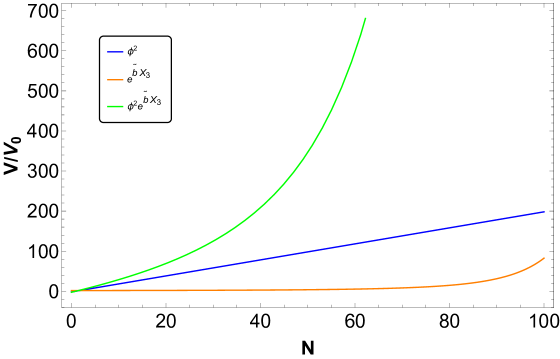
Figure 2: Evolution of the dimensionless PE potential $V(\phi,X_{3})/V_{0}=\phi^{2}\,e^{\tilde{b}X_{3}}$, the terms $\phi^{2}$ and $e^{\tilde{b}X_{3}}$ as a function of the number of $e-$ folds $N$, respectively. Here we have used the values of the parameters $b$ and $X_{3}^{(0)}$ given by Eq.(58).

On the other hand, for the PE potential, the scalar power spectrum as a function of the number of $e-$ folds $N$ from Eq.(28) can be written as

$$\mathcal{P}_{\mathcal{R}}\simeq\frac{16\kappa^{6}\bar{V}_{0}\tilde{V}_{0}e^{\frac{2}{3}b\kappa^{2}X_{3}^{(0)}}\left(\frac{a^{2}}{2\left(\kappa^{2}-2(b-1)b\kappa^{4}X_{3}^{(0)}\right)}+aN\right)^{\frac{a+2}{2}}}{3a\left(4(b-1)b\kappa^{4}NX_{3}^{(0)}-\frac{a}{2(b-1)b\kappa^{2}X_{3}^{(0)}-1}\right)},$$ (55)

and the scalar spectral index in terms of the number $N$ considering Eq.(29) becomes

$$n_{\mathcal{R}}\simeq\frac{4}{9}(27-23b)bX_{3}^{(0)}-\frac{3a}{\frac{a}{2-4(b-1)bX_{3}^{(0)}}+N}.$$ (56)

Additionally, we find that the tensor to scalar ratio $r$ in terms of the number of $e-$ folds $N$ can be written as

$$r\simeq\frac{8a^{2}}{\kappa^{2}\left(\frac{a^{2}}{2\left(\kappa^{2}-2(b-1)b\kappa^{4}X_{3}^{(0)}\right)}+aN\right)}+32(b-1)b\kappa^{2}X_{3}^{(0)}.$$ (57)

Here we have used Eq.(31).

In the following, by simplicity, we will consider the special case in which the power $a$ associated to the power law potential $\bar{V}(\phi)$ is equal to $a=2$, i.e., the chaotic potential $\bar{V}(\phi)\propto\phi^{2}$. Besides, in order to find the parameters $b$, $V_{0}$ ($V_{0}=\bar{V}_{0}\tilde{V}_{0}$) and $X_{3}^{(0)}$ we can consider that the observational parameters; $\mathcal{P}_{\mathcal{R}}$, $n_{\mathcal{R}}$ and the tensor to scalar ratio $r$, when the number of the $e-$folds $N_{*}=60$. In this form, considering that the observational parameters take the values from Planck data[20]; $\mathcal{P}_{\mathcal{R}_{*}}=2.2*10^{-9}$ for the power spectrum, $n_{\mathcal{R}_{*}}=0.967$ and for the tensor scalar ratio $r_{*}=0.04$ (upper bound) at the number of $e-$ folds $N_{*}=60$, then we obtain the following constraints on the parameter-space:

$$b\simeq 0.987,\,\,\,\,\,V_{0}\simeq 5.308\times 10^{-15},\,\,\,\mbox{and}\,\,\,\,\,X_{3}^{(0)}\simeq 0.562,$$ (58)

where we have utilized Eqs.(55), (56) and (57), respectively

In Fig.(2) we show the PE potential $V(\phi,X_{3})/V_{0}$ together with the terms $\phi^{2}$ and $e^{\tilde{b}X_{3}}$ as a function of the number of $e-$ folds $N$. In this plot, we have used the values of $b$ and $X_{3}^{(0)}$ obtained assuming the observational parameters from Planck data, see Eq.(58). In order to write down values of the PE potential $V(\phi,X_{3})/V_{0}$ together the quantities $\phi^{2}$ and $e^{\tilde{b}X_{3}}$ as a function of the number of $e-$folds $N$, we have utilized Eqs.(49),(51) and (53) together with the constraints obtained on $b$ and $X_{3}^{(0)}$. From Fig. (2) we note that during the inflationary epoch in which the number of $e-$ folds $N<70$, the term $\phi^{2}\gg e^{\tilde{b}X_{3}}$ and this suggests that inflation is driven by the term $\phi^{2}$. In this form, we find that the dominant term on the PE potential corresponds to the quadratic term associated to the scalar field $\phi$. In this sense, we can approximate the PE potential during inflation in which $N<70$ as $V(\phi,X_{3})/V_{0}\sim\phi^{2}(1+\tilde{b}X_{3}+..)=\phi^{2}(1+\tilde{b}A^{2}/2+..)$ being the dominant term $\phi^{2}$ in the potential $V(\phi,X_{3})$. It is important to note that in the literature, this approximate potential becomes fundamental in the study of the reheating scenario after inflation, see e.g. Ref.[44].

6 Conclusions

In this paper we have studied an inflationary scenario during the early universe, in the context of a theory described by a scalar field together with a vector field nonminimal coupled to gravity. In this theory, we have obtained the background equations considering a flat FRW metric together with an effective potential associated to both fields. Besides, we have assumed the slow roll approximation in these equations in order to find analytical solutions to the background variables. By using the local field rotation for both fields to recognize the adiabatic and entropy perturbations, we have found the new slow-roll parameters and the observational parameters such as the power spectrum, scalar spectral index, and tensor-to-scalar ratio in our theory.

In order to apply this scenario, we have considered two different effective potentials $V(\phi,X_{3})$. As a first example, we have assumed that the potential associated to both fields does not present interaction between the fields $\phi$ and $X_{3}$, such that, the chosen potential becomes $V(\phi,X_{3})=\bar{V}(\phi)+\tilde{V}(X_{3})$. As a second example, we have considered an effective potential that presents an interaction between both fields and it is given by $V(\phi,X_{3})=\bar{V}(\phi)\,\times\,\tilde{V}(X_{3})$.

For the first example in which the total potential $V(\phi,X_{3})=\bar{V}(\phi)+\tilde{V}(X_{3})$ we have considered that both potentials $\bar{V}(\phi)$ and $\tilde{V}(X_{3})$ correspond to exponential potentials defined by Eq.(35). Under the slow-roll approximation, we have found the relation between the fields $\phi$ and $X_{3}$ given by Eq.(36) in which $X_{3}\propto\phi^{2}$. Also, we have determined the number of $e-$ folds $N$ and the value of the scalar field at the end of the inflationary epoch, see Eqs.(39) and (41), respectively. In order to find the parameters $\bar{V}_{0}$, $\tilde{V}_{0}$ and $X_{3}^{(0)}$, we have assumed the observational parameters in which; the power spectrum $\mathcal{P}_{\mathcal{R}_{*}}=2.2*10^{-9}$, $n_{\mathcal{R}_{*}}=0.967$ and the tensor scalar ratio $r_{*}=0.04$ at the number of $e-$ folds $N_{*}=60$. Here, we have determined that the parameter-space is given by Eq.(45). From these values on the parameters, we have found that the potential associated to the field $X_{3}$ is greater than $\bar{V}(\phi)$, i.e., $\tilde{V}(X_{3})>V(\phi)$ as shown in Fig.(1). In this context, we have found that the inflationary scenario is driven by the field $X_{3}$ through its exponential potential $\tilde{V}(X_{3})\sim V(\phi,X_{3})\simeq H^{2}$.

As a second example we have analyzed an effective potential $V(\phi,X_{3})$ defined as the product $V(\phi,X_{3})=\bar{V}(\phi)\times\tilde{V}(X_{3})$. In particular, we have assumed a chaotic potential for the scalar field $\phi$ and an exponential potential for the field $X_{3}$ (see Eq.(49)) and this total potential is known in the literature as product-exponential potential or PE potential. By considering the slow-roll approximation, we have obtained the relation between the fields $\phi$ and $X_{3}$ given by Eq.(51). Besides, we have found the number of $e-$ folds $N$ and the value of the scalar field at the end of the inflationary epoch, as in the previous example. As before, we have obtained the constraints on the parameter-space considering the observational parameters. In particular we have found the constraints on the parameters $b$, $V_{0}$ and the integration constant $X_{3}^{(0)}$, see Eq.(58). From Fig. (2) we have found that during the inflationary epoch in which the number of $e-$ folds $N<70$, the term $\phi^{2}\gg e^{\tilde{b}X_{3}}$ and this suggests that inflation is driven by the term $\phi^{2}$. In this sense, we have found that the dominant term on the PE potential corresponds to the quadratic term associated to the scalar field $\phi$. In this context, we notice that the PE potential during inflation can be approximate to $V(\phi,X_{3})/V_{0}\sim\phi^{2}(1+\tilde{b_{3}}X_{3}+..)=\phi^{2}(1+\tilde{b_{3}}A^{2}/2+..)$ as the potential studied in theory of reheating after inflation, in which the interaction potential is proportional to $\phi^{2}\,A^{2}$.

Finally, in this article, we have not addressed the inflationary scenario in a scalar vector gravity theory for other types of effective potential $V(\phi,X_{3})$, see e.g.[45, 46]. We hope to return to this point in the near future.

7 Acknowledgments

M. Gonzalez-Espinoza acknowledges the financial support of FONDECYT de Postdoctorado, N° 3230801.

References

- [1] A. H. Guth, Phys. Rev. D 23, 347-356 (1981). doi:10.1103/PhysRevD.23.347.
- [2] A. D. Linde, Phys. Lett. B 108, 389-393 (1982). doi:10.1016/0370-2693(82)91219-9.
- [3] V. Mukhanov, Cambridge University Press, 2005, ISBN 978-0-521-56398-7 doi:10.1017/CBO9780511790553
- [4] R. R. Caldwell and P. J. Steinhardt, Phys. Rev. D 57, 6057-6067 (1998). doi:10.1103/PhysRevD.57.6057.
- [5] F. Vernizzi, Phys. Rev. D 69, 083526 (2004). doi:10.1103/PhysRevD.69.083526.
- [6] D. Langlois, Phys. Rev. D 59 (1999), 123512 doi:10.1103/PhysRevD.59.123512 [arXiv:astro-ph/9906080 [astro-ph]].
- [7] D. Langlois and S. Renaux-Petel, JCAP 04 (2008), 017 doi:10.1088/1475-7516/2008/04/017 [arXiv:0801.1085 [hep-th]].
- [8] D. Seery and J. E. Lidsey, JCAP 0509, 011 (2005). doi:10.1088/1475-7516/2005/09/011.
- [9] N. Arkani-Hamed, H. C. Cheng, P. Creminelli and L. Randall, Phys. Rev. Lett. 90, 221302 (2003). doi:10.1103/PhysRevLett.90.221302.
- [10] D. Baumann, doi:10.1142/9789814327183_0010 [arXiv:0907.5424 [hep-th]].
- [11] D. H. Lyth and A. R. Liddle, Cambridge university press, 2009.
- [12] V. F. Mukhanov, H. A. Feldman and R. H. Brandenberger, Phys. Rept. 215 (1992), 203-333 doi:10.1016/0370-1573(92)90044-Z
- [13] A. D. Linde, Phys. Lett. B 114 (1982), 431-435 doi:10.1016/0370-2693(82)90086-7
- [14] A. A. Starobinsky and J. Yokoyama, [arXiv:gr-qc/9502002 [gr-qc]].
- [15] Z. Lalak, D. Langlois, S. Pokorski and K. Turzynski, JCAP 07 (2007), 014 doi:10.1088/1475-7516/2007/07/014 [arXiv:0704.0212 [hep-th]].
- [16] R. H. Brandenberger, A. R. Frey and L. C. Lorenz, Int. J. Mod. Phys. A 24 (2009), 4327-4354 doi:10.1142/S0217751X09045509 [arXiv:0712.2178 [hep-th]].
- [17] A. Golovnev, V. Mukhanov and V. Vanchurin, JCAP 06, 009 (2008). doi:10.1088/1475-7516/2008/06/009.
- [18] Dimopoulos, K., Karciauskas, M., Lyth, D.H., Rodriguez, Y. Journal of Cosmology and Astroparticle Physics 2009.05 (2009): 1-15.
- [19] Golovnev, A., Mukhanov, V., Vanchurin, V. ”Vector Inflation.” Journal of High Energy Physics 2009.06 (2009): 1-37.
- [20] Planck Collaboration, N. Aghanim et al., Astron. Astrophys. 641, A6 (2020). doi:10.1051/0004-6361/201833910.
- [21] P. A. R. Ade et al. [Planck Collaboration], Astron. Astrophys. 594, A13 (2016). doi:10.1051/0004-6361/201525830.
- [22] S. Alam et al. [BOSS Collaboration], Mon. Not. Roy. Astron. Soc. 470, no. 3, 2617-2652 (2017). doi:10.1093/mnras/stx721.
- [23] A. J. Ross et al., Mon. Not. Roy. Astron. Soc. 449, no. 1, 835-847 (2015). doi:10.1093/mnras/stv154.
- [24] B. P. Abbott et al. [LIGO Scientific and Virgo], Phys. Rev. Lett. 116, no. 6, 061102 (2016). doi:10.1103/PhysRevLett.116.061102.
- [25] R. N. Lerner and J. McDonald, Phys. Rev. D 70, 123522 (2004). doi:10.1103/PhysRevD.70.123522.
- [26] S. H. H. Tye and I. Wasserman, Phys. Rev. D 71, 103508 (2005). doi:10.1103/PhysRevD.71.103508.
- [27] L. Heisenberg, R. Kase and S. Tsujikawa, Phys. Rev. D 98, no.2, 024038 (2018) doi:10.1103/PhysRevD.98.024038 [arXiv:1805.01066 [gr-qc]].
- [28] L. Heisenberg, JCAP 10, 054 (2018) doi:10.1088/1475-7516/2018/10/054 [arXiv:1801.01523 [gr-qc]].
- [29] A. Taruya and Y. Nambu, Phys. Lett. B 428, 37-43 (1998) doi:10.1016/S0370-2693(98)00378-5 [arXiv:gr-qc/9709035 [gr-qc]].
- [30] D. Wands, N. Bartolo, S. Matarrese and A. Riotto, Phys. Rev. D 66, 043520 (2002) doi:10.1103/PhysRevD.66.043520 [arXiv:astro-ph/0205253 [astro-ph]].
- [31] C. Gordon, D. Wands, B. A. Bassett and R. Maartens, Phys. Rev. D 63, 023506 (2000) doi:10.1103/PhysRevD.63.023506 [arXiv:astro-ph/0009131 [astro-ph]].
- [32] A. R. Liddle and D. H. Lyth, doi:10.1017/CBO9781139175180.
- [33] A. Riotto, ICTP Lect. Notes Ser. 14, 317-413 (2003) [arXiv:hep-ph/0210162 [hep-ph]].
- [34] F. Vernizzi and D. Wands, JCAP 05, 019 (2006) doi:10.1088/1475-7516/2006/05/019 [arXiv:astro-ph/0603799 [astro-ph]].
- [35] T. Battefeld and R. Easther, JCAP 03, 020 (2007) doi:10.1088/1475-7516/2007/03/020 [arXiv:astro-ph/0610296 [astro-ph]].
- [36] E. J. Copeland, A. R. Liddle and D. Wands, Phys. Rev. D 57, 4686-4690 (1998) doi:10.1103/PhysRevD.57.4686 [arXiv:gr-qc/9711068 [gr-qc]].
- [37] F. Lucchin and S. Matarrese, Phys. Rev. D 32, 1316 (1985) doi:10.1103/PhysRevD.32.1316.
- [38] Abramowitz, Milton; Irene Stegun (1964). Handbook of Mathematical Functions with Formulas, Graphs, and Mathematical Tables. Abramowitz and Stegun. New York.
- [39] J. Garcia-Bellido and D. Wands, Phys. Rev. D 53, 5437-5445 (1996) doi:10.1103/PhysRevD.53.5437 [arXiv:astro-ph/9511029 [astro-ph]].
- [40] C. T. Byrnes, K. Y. Choi and L. M. H. Hall, JCAP 10, 008 (2008) doi:10.1088/1475-7516/2008/10/008 [arXiv:0807.1101 [astro-ph]].
- [41] I. Huston and A. J. Christopherson, [arXiv:1302.4298 [astro-ph.CO]].
- [42] J. Elliston, D. J. Mulryne, D. Seery and R. Tavakol, JCAP 11, 005 (2011) doi:10.1088/1475-7516/2011/11/005 [arXiv:1106.2153 [astro-ph.CO]].
- [43] P. González, G. A. Palma and N. Videla, JCAP 12, 001 (2018) doi:10.1088/1475-7516/2018/12/001 [arXiv:1805.10360 [hep-th]].
- [44] L. Kofman, A. D. Linde and A. A. Starobinsky, Phys. Rev. Lett. 73, 3195-3198 (1994) doi:10.1103/PhysRevLett.73.3195 [arXiv:hep-th/9405187 [hep-th]]; A. Albrecht, P. J. Steinhardt, M. S. Turner and F. Wilczek, Phys. Rev. Lett. 48, 1437 (1982) doi:10.1103/PhysRevLett.48.1437; L. Kofman, A. D. Linde and A. A. Starobinsky, Phys. Rev. D 56, 3258-3295 (1997) doi:10.1103/PhysRevD.56.3258 [arXiv:hep-ph/9704452 [hep-ph]]; E. I. Guendelman, R. Herrera and P. Labrana, Phys. Rev. D 103, 123515 (2021) doi:10.1103/PhysRevD.103.123515 [arXiv:2005.14151 [gr-qc]].
- [45] A. A. Starobinsky, S. Tsujikawa and J. Yokoyama, Nucl. Phys. B 610, 383-410 (2001) doi:10.1016/S0550-3213(01)00322-4 [arXiv:astro-ph/0107555 [astro-ph]].
- [46] C. T. Byrnes and G. Tasinato, JCAP 08, 016 (2009) doi:10.1088/1475-7516/2009/08/016 [arXiv:0906.0767 [astro-ph.CO]]; F. Bernardeau and J. P. Uzan, Phys. Rev. D 66, 103506 (2002) doi:10.1103/PhysRevD.66.103506 [arXiv:hep-ph/0207295 [hep-ph]]; E. Guendelman, R. Herrera and D. Benisty, Phys. Rev. D 105, no.12, 124035 (2022) doi:10.1103/PhysRevD.105.124035 [arXiv:2201.06470 [gr-qc]].