PhiNets: Brain-inspired Non-contrastive Learning
Based on Temporal Prediction Hypothesis

Satoki Ishikawa Tokyo Institute of Technology Okinawa Institute of Science and Technology Equal contribution Makoto Yamada Okinawa Institute of Science and Technology Equal contribution Corresponding author: makoto.yamada@oist.jp Han Bao Kyoto University Okinawa Institute of Science and Technology Yuki Takezawa Kyoto University Okinawa Institute of Science and Technology
Abstract

SimSiam is a prominent self-supervised learning method that achieves impressive results in various vision tasks under static environments. However, it has two critical issues: high sensitivity to hyperparameters, especially weight decay, and unsatisfactory performance in online and continual learning, where neuroscientists believe that powerful memory functions are necessary, as in brains. In this paper, we propose PhiNet, inspired by a hippocampal model based on the temporal prediction hypothesis. Unlike SimSiam, which aligns two augmented views of the original image, PhiNet integrates an additional predictor block that estimates the original image representation to imitate the CA1 region in the hippocampus. Moreover, we model the neocortex inspired by the Complementary Learning Systems theory with a momentum encoder block as a slow learner, which works as long-term memory. We demonstrate through analysing the learning dynamics that PhiNet benefits from the additional predictor to prevent the complete collapse of learned representations, a notorious challenge in non-contrastive learning. This dynamics analysis may partially corroborate why this hippocampal model is biologically plausible. Experimental results demonstrate that PhiNet is more robust to weight decay and performs better than SimSiam in memory-intensive tasks like online and continual learning.

1 Introduction

There are notable differences between biological brains and deep neural networks. These differences can be divided into two categories: differences in learning algorithms—brains do not perform backpropagation [18, 1, 31]—and structural differences—brains have both the neocortex and hippocampus, but most of the existing models are relevant only to either of them [39, 47]. In this paper, we focus on structural differences to explore better architectures of self-supervised representation learning. While CNNs with skip connections such as ResNets can be interpreted to approximate the visual cortex [49, 26], they lack the intricate hippocampal structure. Thus, neural networks are still inferior to brains in tasks where memory matters, such as continual and online learning.

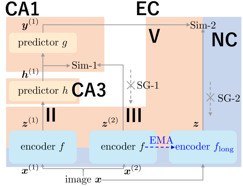
How can we bring deep neural networks closer to the structure of brains? To address the question, we propose a self-supervised learning (SSL) algorithm based on the temporal prediction hypothesis and the Complementary Learning Systems (CLS) theory [30]. We begin by examining predictive coding, which supposes that brains use predictions based on prior experiences to interpret sensory information efficiently [32, 40, 14]. Temporal prediction hypothesis is an extended framework supposing that the hippocampus learns from signals with temporal differences based on predictive coding [12]. As an effective framework for realising temporal prediction hypothesis in deep neural networks, we employ SimSiam [11] as a backbone model, which is a representative non-contrastive learning method in computer vision and shows impressive performance across diverse tasks, including imbalanced classification [27], detection, segmentation [11], and reinforcement learning [45]. Building on this, we propose a new network architecture called PhiNet. Specifically, PhiNet is inspired by a hippocampal modelling framework: the cortex acts as an encoder, the CA3 region serves as a predictor, and the CA1 region uses a loss function and an additional predictor block to quantify the prediction errors (see Figure 1(c)). In addition, we incorporate StopGradient mechanisms in SimSiam to simulate temporal difference learning, allowing the model to refine its predictions iteratively based on feedback experiences.

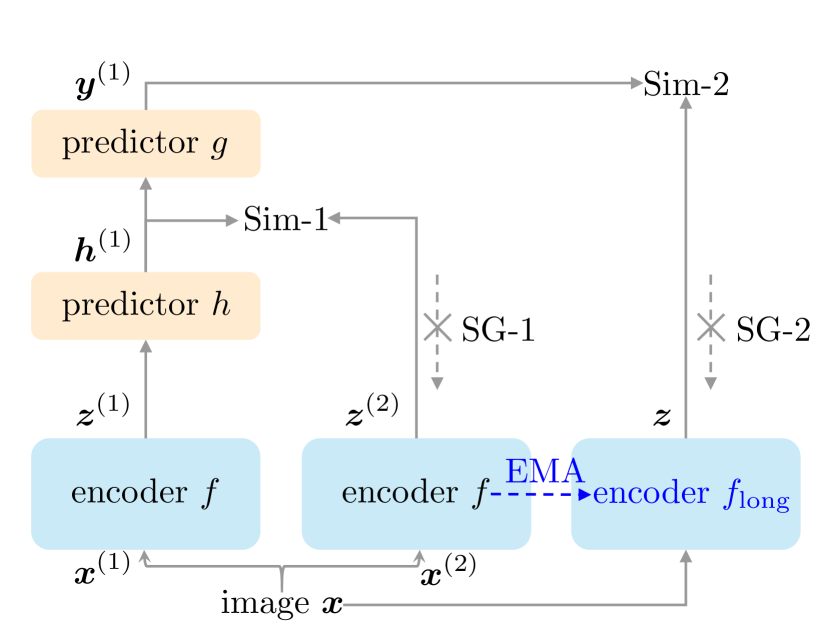
In addition to the hippocampus, the neocortex plays another crucial role in brains. We jointly model the neocortex and hippocampus based on CLS theory [30, 24]. CLS theory assumes two brain learning systems: the hippocampus for short-term memory and the neocortex for long-term memory, with the latter updating more slowly yet stably. In neural networks, recent work witnessed that supervised continual learning performance improves by integrating fast and slow learning systems [36, 35, 2, 38]. Therefore, we implement a slow mechanism in PhiNet to store previous information. Our proposed method, X-PhiNet, leverages the momentum encoder to store information in the neocortex model from the hippocampus model.

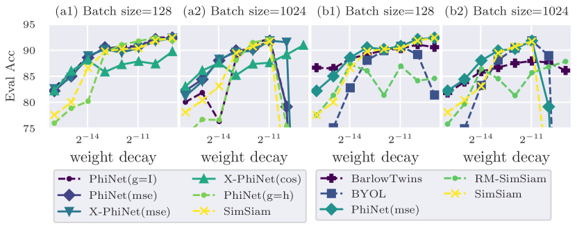
Experimental validation and theoretical analysis demonstrate the effectiveness of PhiNet. Firstly, our systematic experiments indicate that PhiNet achieves performance comparable to SimSiam but with greater robustness to weight decay (see Figure 5). Interestingly, the hyperparameter robustness can be partially observed through eigenvalue analysis in dynamical systems [46]. Our theoretical analysis (in Section 4) shows that the learning dynamics of SimSiam is sensitive to initialization and may easily collapse when weight decay intensity is not chosen appropriately, but the PhiNet-dynamics is more resilient (C1). This theoretical analysis provides an interesting and plausible explanation of why the interplay between two predictors is important not only in self-supervised learning but also in the temporal prediction hypothesis. Secondly, experimental results in Table 2 show that X-PhiNet performs well in online and continual learning, where memory architectures matter significantly and brains are superior to artificial neural networks. By leveraging insights from cognitive neuroscience, PhiNet introduces a novel perspective to SSL, offering a pathway towards more efficient and effective SSL methodologies that harness the power of both augmented and original image data.

Contributions.

  • Section 3: we propose a new non-contrastive learning method called PhiNet, which is inspired by a hippocampal model [12].

  • Section 4: we compare the learning dynamics [46] of PhiNet and SimSiam. Consequently, it elucidates that PhiNet can avoid the complete collapse of representations [28, 4] more easily than SimSiam with the aid of the additional predictor.

  • Section 5.1: we investigate the image classification performance of PhiNet using CIFAR and ImageNet datasets. We show that PhiNet performs comparably to SimSiam but is more robust against weight decay.

  • Section 5.2: we further extend PhiNet by proposing X-PhiNet to integrate the neocortex model based on the Complementary Learning Systems (CLS) theory [30]. Experimentally, X-PhiNet works effectively in online and continual learning.

2 Related Work

Brain-inspired methods.

Predictive coding, initially introduced as a theory of the retina [44], has gained attention as a unifying theory of cortical functions [32, 40, 14]. They suggest that brains operate by predicting sensory inputs at various levels of abstraction to minimise prediction errors. Recent studies have leveraged these ideas for contrastive learning [34, 19]. Chen et al. [12] extended the predictive coding theory to the hippocampus with the temporal prediction hypothesis. Specifically, the temporal prediction hypothesis supposes that prediction errors are calculated with the CA1 model and used to update the CA3 model. Some studies have attempted to apply the hippocampus model to representation learning [35, 37]. Among them, DualNet refines representation learning based on CLS theory [30, 24], which supposes that the interplay between slow (supervised) and fast (self-supervised) architectures is the basis of brain learning. Pham et al. [35] examined supervised learning tasks alongside self-supervised training, while Chen et al. [12] explored SSL using time-series data, which has practical limitations. Our study stands on CLS theory to propose a method that does not require either label information or time-series data.

Self-supervised learning.

Current mainstream approaches to self-supervised learning (SSL) often rely on cross-view prediction frameworks [6], with contrastive learning emerging as a prominent SSL paradigm. In contrastive learning like SimCLR [10], models contrast positive (similar) and negative (dissimilar) samples to learn data representations. One limitation of SimCLR is its empirical reliance on gigantic negative samples, which has been theoretically articulated [5, 3]. To address this issue, recent research has focused on approaches free from negative sampling [16, 8, 9]. For instance, BYOL [16] trains representations by aligning online and target networks, where the target network is created by maintaining a moving average of the online network parameters. SimSiam [11] utilises a Siamese network to align two augmented views of an input by fixing one of the networks with StopGradient. While the lack of negative samples may easily yield collapsed representations, namely, constant representation, Tian et al. [46] analysed the BYOL/SimSiam dynamics with a two-layer network and found that complete collapse is prevented unless weight decay is excessively strong. We partially leverage their analysis framework to explain the mechanism of our PhiNet. In recent years, many studies have been leveraging SimSiam for continual learning [43, 29] and reinforcement learning [45]. RM-SimSiam enhances the performance of continual learning by incorporating a memory block into SimSiam [15], while its architecture has not been neuroscientifically grounded.

Refer to caption
(a) PhiNet architecture.
Refer to caption
(b) X-PhiNet architecture.
Refer to caption
(c) Interpretation of X-PhiNet.
Figure 1: The architecture of PhiNet and its interpretation as a hippocampal model. EMA in the X-PhiNet model stands for the exponential moving average, and NC in Figure 1(c) stands for NeoCortex. The architecture originates from a single input, branches out into three paths, and then compares the similarity of all paths in Sim-2. Thus, we call it PhiNet ($\Phi$-Net) because the shape of the architecture resembles the Greek letter Phi ($\Phi$).

3 PhiNets ($\Phi$-Nets)

In this paper, we propose PhiNets, which are non-contrastive methods based on CLS theory [30] and the temporal prediction hypothesis [12]. Chen et al. [12, Figure 1] provides the hippocampal model, where the entorhinal cortex (EC) serves as an input signal layer, the CA3 region serves as the predictor, and the CA1 region measures the prediction error. The CA3 region receives an input signal from the EC and recurrently forecasts future signals. The prediction output of CA3 is propagated to the CA1 region, which computes the discrepancy between the CA3 prediction and the EC input and refines the internal model stored in CA3. Compensating the temporal differences between EC–CA3 and EC–CA1 is hypothesised to facilitate the learning and replay of temporal sequences in the hippocampus.

Whereas Chen et al. [12] tested this model to replicate recorded neural activities through simulation, we develop a self-supervised learner PhiNet based on this hypothesis as follows:

  • We use deep encoders $f$ and/or $f_{\text{long}}$ to represent cortex.

  • We model CA3 by a predictor network.

  • We model CA1 by combining a loss function and another predictor.

  • We train the model by jointly minimizing the loss for the hippocampus and the neocortex models.

  • The long-term memory is implemented by an exponential moving average with compression.

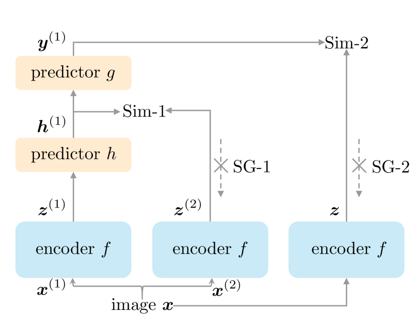
Figures 1(a) and 1(b) depict the architecture of PhiNets, while Figure 1(c) illustrates how PhiNet can be interpreted as a hippocampal model [12] under the temporal prediction hypothesis.

Note that our approach diverges from the temporal prediction hypothesis method proposed by Chen et al. [12]. Specifically, while they assume an image sequence as input, we consider pairs of augmented signals alongside their original inputs thanks to the StopGradient operator, expanding the applicability of hippocampal models to standard vision tasks.

3.1 Hippocampal Modelling under Temporal Prediction Hypothesis

The hippocampal model consists of the EC, CA3, and CA1, each of which we describe below.

Modelling of EC layer.

The entorhinal cortex (EC) is the main input and output cortex of the hippocampus [12]. Let us denote the original input as ${\bm{x}}_{i}\in\mathbb{R}^{{d}}$. We model that the hippocampus model has two augmented signals from the original input as ${\bm{x}}_{i}^{(1)}\in\mathbb{R}^{{d}}$ and ${\bm{x}}_{i}^{(2)}\in\mathbb{R}^{{d}}$, in addition to the original input ${\bm{x}}_{i}$. Let $f:\mathbb{R}^{{d}}\to\mathbb{R}^{m}$ denote the encoder. Then, the cortical representation in the EC is given as follows:

$\displaystyle{\bm{z}}_{i}^{(1)}=f({\bm{x}}_{i}^{(1)}),\quad{\bm{z}}_{i}^{(2)}=f({\bm{x}}_{i}^{(2)}),\quad\text{and}\quad{\bm{z}}_{i}=f({\bm{x}}_{i}).$

We regard each corresponding to the layers II, III, and V of the EC in Chen et al. [12, Figure 1]. Thus, for self-supervised training, we have the size-$n$ triplet dataset ${\mathcal{D}}=\{({\bm{x}}_{i}^{(1)},{\bm{x}}_{i}^{(2)},{\bm{x}}_{i})\}_{i=1}^{n}$. The hippocampal learning can be characterized as a learning problem of the encoder $f$ from the training dataset ${\mathcal{D}}$.

Modelling of CA3 region.

The CA3 region is responsible for predicting future signals:

$\displaystyle{\bm{h}}_{i}^{(1)}$ $\displaystyle=h({\bm{z}}_{i}^{(1)}),~{}~{}~{}~{}~{}{\bm{h}}_{i}^{(2)}=h({\bm{z}}_{i}^{(2)}),$

where $h:\mathbb{R}^{m}\rightarrow\mathbb{R}^{m}$ is the predictor network. We implement the predictor with a two-layer neural network with the ReLU activation and batch normalization.

Modelling of CA1 region.

CA1 measures the difference between the predicted signal and its future signal. In this paper, we model CA1 by a mixture of a loss function and a predictor, while Chen et al. [12] uses only MSE loss for modelling CA1. We use the symmetric negative cosine loss function to measure the temporally distant signal ${\bm{z}}_{i}^{(2)}$ (layer III of EC) and the predicted representation from CA3 ${\bm{h}}_{i}^{(1)}=h({\bm{z}}_{i}^{(1)})$:

$\displaystyle L_{\textnormal{Cos}}({\bm{\theta}})\!=\!-\frac{1}{2n}\sum_{i=1}^{n}\!\frac{({\bm{h}}_{i}^{(1)})^{\top}\bar{{\bm{z}}}_{i}^{(2)}}{\|{\bm{h}}_{i}^{(1)}\|_{2}\|\bar{{\bm{z}}}_{i}^{(2)}\|_{2}}-\frac{1}{2n}\sum_{i=1}^{n}\!\frac{(\bar{{\bm{z}}}_{i}^{(1)})^{\top}{\bm{h}}_{i}^{(2)}}{\|\bar{{\bm{z}}}_{i}^{(1)}\|_{2}\|{{\bm{h}}}_{i}^{(2)}\|_{2}},$

where ${\bm{\theta}}$ represent the entire model parameter and $\bar{{\bm{z}}}_{i}^{(1)}\coloneqq{\textnormal{SG}}({\bm{z}}_{i}^{(1)})\in\mathbb{R}^{m}$ is a latent variable with StopGradient, in which the gradient update shall not be executed.

Remark that StopGradient yields a “temporal difference”, for which we can interpret SimSiam as a hippocampus model. Let us look closely at Sim-1 in Figure 1(b), equivalent to SimSiam. We let $f_{t}$ denote the encoder $f$ at time $t$. The left path of Sim-1 can then be expressed as ${\bm{h}}^{(1)}=h(f_{t}({\bm{x}}))$. As the right path of Sim-1 is adapted with StopGradient, it can be written as ${\bm{z}}^{(2)}={\textnormal{SG}}(f({\bm{x}}))=f_{t-1}({\bm{x}}(t))$. Eventually, Sim-1 aligns $f_{t}({\bm{x}})$ and $f_{t-1}({\bm{x}})$ by the predictor $h$. This Sim-1 interpretation indicates that PhiNet predicts past signals, which slightly deviates from the original temporal prediction hypothesis [12] supposing that CA3 is in charge of predicting future signals.

In addition to measuring the difference, the CA1 region outputs the signal to the EC (V layer). Thus, we model the output of CA1 as follows:

$\displaystyle{{\bm{y}}}_{i}^{(1)}=g({\bm{h}}_{i}^{(1)}),\quad{{\bm{y}}}_{i}^{(2)}=g({\bm{h}}_{i}^{(2)}),$

where $g:\mathbb{R}^{m}\to\mathbb{R}^{m}$ is another predictor network. As we will see soon, CLS theory supposes that this feedback from CA1 to the EC eventually propagates to the neocortex (NC), which is stored in long-term memory.

3.2 X-PhiNet: Slow and Fast Learning with Complementary Learning Systems (CLS) Theory

The hippocampus and neocortex play crucial roles in brain cognition. For effective long-term memory storage, it is essential to transfer information from the hippocampus to the NC. We first aim to formulate the joint learning of the hippocampus and NC models. Then, we propose using the exponential moving average (EMA) to transfer model parameters from short-term to long-term memory, with the goal of compressing the original input signal.

In the EC layer, we model the update of the encoder function by using the output of CA1 and the representation ${\bm{z}}_{i}=f({\bm{x}}_{i})$ (V layer of EC). Then, the loss function can be given as follows:

$\displaystyle L_{\textnormal{NC}}({\bm{\theta}})\!=\!\frac{1}{2n}\sum_{i=1}^{n}\|{{\bm{y}}}_{i}^{(1)}-{\textnormal{SG}}({\bm{z}}_{i})\|_{2}^{2}+\frac{1}{2n}\sum_{i=1}^{n}\|{\bm{y}}_{i}^{(2)}-{\textnormal{SG}}({\bm{z}}_{i})\|_{2}^{2}.$

This is regarded as slow learning. Finally, the whole objective function of PhiNet is given as

$\displaystyle L({\bm{\theta}})=\underbrace{L_{\textnormal{Cos}}({\bm{\theta}})}_{\textnormal{ Hippocampus loss}}+\underbrace{L_{\textnormal{NC}}({\bm{\theta}})}_{\textnormal{Neocortex loss}}.$

We then minimise $L({\bm{\theta}})$ to learn the hippocampus and the NC models. The optimisation can be efficiently performed using backpropagation. It is worth noting that we can utilise different loss functions for Sim-1 and/or Sim-2 in PhiNet. In this paper, we set Sim-1 to negative cosine similarity and Sim-2 to either MSE or negative cosine similarity.

Exponential moving average.

The original PhiNet formulation employs the same encoder for both the short-term and long-term memories for simplicity (Section 3.2). However, CLS theory claims that a natural architecture should have fast and slow mechanisms to store information. To this end, we introduce the following stable encoder for long-term memory:

$\displaystyle{\bm{z}}_{i}=f_{\textnormal{long}}({\bm{x}}_{i}).$

Then, we solve the PhiNet optimisation problem by minimising both $L_{\textnormal{NC}}({\bm{\theta}})$ and $L_{\textnormal{Cos}}({\bm{\theta}})$ using the exponential moving average (EMA) of the model parameters of $f$ and $f_{\textnormal{long}}$ as

$\displaystyle{\bm{\xi}}\leftarrow\beta{\bm{\xi}}+(1-\beta){\bm{\xi}}_{\textnormal{long}},$

where ${\bm{\xi}}$ and ${\bm{\xi}}_{\textnormal{long}}$ are the model parameters of $f$ and $f_{\textnormal{long}}$, respectively, and $\beta\in[0,1]$ is a hyperparameter. Model parameters persist in $f_{\textnormal{long}}$ more stably than the original encoder $f$, which facilitates slow learning. We call this method as X-PhiNet.

4 What We Benefit from Additional Predictor: Dynamics Perspective

When PhiNet is compared with SimSiam, the additional predictor $g$ in CA1 is peculiar. We study the learning dynamics of PhiNet with a toy model. Despite its simplicity, dynamics analysis is beneficial in showcasing how the predictor $g$ enhances learning.

Analysis model.

Let us specify the analysis model, following Tian et al. [46]. The $d$-dimensional input is sampled from the isotropic normal ${\bm{x}}\sim{\mathcal{N}}({\bm{0}},{\mathbf{I}})$ and augmented by the isotropic normal ${\bm{x}}^{(1)},{\bm{x}}^{(2)}\sim{\mathcal{N}}({\bm{x}},\sigma^{2}{\mathbf{I}})$, where $\sigma^{2}$ indicates the strength of data augmentation. The encoder $f$ and predictors $g$ and $h$ are modelled by linear networks without bias: $f({\bm{x}})\coloneqq{\mathbf{W}}_{f}{\bm{x}}$, $g({\bm{h}})\coloneqq{\mathbf{W}}_{g}{\bm{h}}$, and $h({\bm{z}})\coloneqq{\mathbf{W}}_{h}{\bm{z}}$, where ${\mathbf{W}}_{f}\in\mathbb{R}^{m\times{d}}$ and ${\mathbf{W}}_{g},{\mathbf{W}}_{h}\in\mathbb{R}^{m\times m}$. The predictors $h$ and $g$ transform latents ${\bm{z}}^{(1)},{\bm{h}}^{(1)}\in\mathbb{R}^{h}$ into ${\bm{h}}^{(1)},{\bm{y}}^{(1)}\in\mathbb{R}^{m}$ with the same dimension $m$ to predict the other noisy latent ${\bm{z}}^{(2)}$ and the noise-free latent ${\bm{z}}$, respectively (see Figure 1(a)).

Unlike $L_{\textnormal{Cos}}$ introduced in Section 3, we focus on the (not symmetrised) MSE loss for measuring the discrepancy between ${\bm{h}}^{(1)}$ and ${\bm{z}}^{(2)}$ for the transparency of analysis. Interested readers may refer to Halvagal et al. [17] and Bao [4] for further extension to incorporate the cosine loss into the SimSiam dynamics. Consequently, the expected loss function of PhiNet $\overline{L}({\mathbf{W}}_{f},{\mathbf{W}}_{g},{\mathbf{W}}_{h})$ is given as follows:

$$\overline{L}\coloneqq\frac{1}{2}\mathbb{E}_{{\bm{x}}}\mathbb{E}_{{\bm{x}}^{(1)},{\bm{x}}^{(2)}|{\bm{x}}}\left[\|{\mathbf{W}}_{h}{\mathbf{W}}_{f}{\bm{x}}^{(1)}-{\textnormal{SG}}({\mathbf{W}}_{f}{\bm{x}}^{(2)})\|^{2}+\|{\mathbf{W}}_{g}{\mathbf{W}}_{h}{\mathbf{W}}_{f}{\bm{x}}^{(1)}-{\textnormal{SG}}({\mathbf{W}}_{f}{\bm{x}})\|^{2}\right].$$

We will analyse the gradient flow $\dot{\mathbf{W}}_{\{f,g,h\}}=-\nabla\overline{L}-\rho{\mathbf{W}}_{\{f,g,h\}}$ ($\rho>0$: weight decay intensity) subsequently. The gradient flows are derived as follows (see Appendix C.1):

$\displaystyle\dot{\mathbf{W}}_{f}$ $\displaystyle=-{\mathbf{W}}_{h}^{\top}\{(1+\sigma^{2})({\mathbf{I}}+{\mathbf{W}}_{g}^{\top}{\mathbf{W}}_{g}){\mathbf{W}}_{h}-({\mathbf{I}}+{\mathbf{W}}_{g}^{\top})\}{\mathbf{W}}_{f}-\rho{\mathbf{W}}_{f},$
$\displaystyle\dot{\mathbf{W}}_{g}$ $\displaystyle=-\{(1+\sigma^{2}){\mathbf{W}}_{h}-{\mathbf{I}}\}{\mathbf{W}}_{f}{\mathbf{W}}_{f}^{\top}{\mathbf{W}}_{h}^{\top}-\rho{\mathbf{W}}_{g},$
$\displaystyle\dot{\mathbf{W}}_{h}$ $\displaystyle=-\{(1+\sigma^{2})({\mathbf{I}}+{\mathbf{W}}_{g}^{\top}{\mathbf{W}}_{g}){\mathbf{W}}_{h}-({\mathbf{I}}+{\mathbf{W}}_{g}^{\top})\}{\mathbf{W}}_{f}{\mathbf{W}}_{f}^{\top}-\rho{\mathbf{W}}_{h}.$
Refer to caption
Refer to caption
Refer to caption
Refer to caption
Figure 2: State space diagrams of PhiNet dynamics with different levels of weight decay: strong ($\rho=0.12$), medium ($\rho=0.03$), light ($\rho=0.003$), and weak ($\rho=0.0001$). The vector fields are numerically computed with $\sigma^{2}=1.5$. The state space bifurcates at the boundary of each level. The nullclines are shown with the green real ($\dot{\psi}=0$) and dotted ($\dot{\gamma}=0$) lines. The red dots are sinks.

Eigenvalue dynamics.

The matrix dynamics we have derived are rigorous but not amenable to further analysis. Here, we decouple the matrix dynamics into the eigenvalue dynamics. Let ${\bm{\Phi}}\coloneqq{\mathbf{W}}_{f}{\mathbf{W}}_{f}^{\top}\in\mathbb{R}^{m\times m}$. Following Tian et al. [46, Theorem 3] and Bao [4, Proposition 1], we can show that the eigenspaces of ${\bm{\Phi}}$, ${\mathbf{W}}_{g}$, and ${\mathbf{W}}_{h}$ quickly align as $t$ increases (see Appendix C.2). Therefore, we assume the following conditions:

  1. (A1)

    ${\mathbf{W}}_{g}$ and ${\mathbf{W}}_{h}$ are symmetric.

  2. (A2)

    The eigenspaces of ${\bm{\Phi}}$, ${\mathbf{W}}_{g}$, and ${\mathbf{W}}_{h}$ align for every time step $t$.

Under these assumptions, ${\bm{\Phi}}$, ${\mathbf{W}}_{g}$, and ${\mathbf{W}}_{h}$ are simultaneously diagonalizable and can be written as ${\bm{\Phi}}={\mathbf{U}}{\bm{\Lambda}}_{\Phi}{\mathbf{U}}^{\top}$, ${\mathbf{W}}_{g}={\mathbf{U}}{\bm{\Lambda}}_{g}{\mathbf{U}}^{\top}$, and ${\mathbf{W}}_{h}={\mathbf{U}}{\bm{\Lambda}}_{h}{\mathbf{U}}^{\top}$, where ${\mathbf{U}}$ is the (time-dependent) common orthogonal eigenvectors. Here, ${\bm{\Lambda}}_{\Phi}=\operatorname{\mathrm{diag}}[\phi_{1},\dots,\phi_{m}]$, ${\bm{\Lambda}}_{g}=\operatorname{\mathrm{diag}}[\gamma_{1},\dots,\gamma_{m}]$, and ${\bm{\Lambda}}_{h}=\operatorname{\mathrm{diag}}[\psi_{1},\dots,\psi_{m}]$ are the corresponding eigenvalues. Noting that the dynamics quickly fall on to $\phi(t)=\psi(t)^{2}$, we can decouple the matrix dynamics into the eigenvalue dynamics of $(\psi,\gamma)$ only (shown in Appendix C.3 and C.4):

$$\text{(PhiNet-dynamics)}\qquad\begin{cases}\dot{\psi}&=\{(1+\gamma)-(1+\sigma^{2})(1+\gamma^{2})\psi\}\psi^{2}-\rho\psi,\\ \dot{\gamma}&=\{1-(1+\sigma^{2})\psi\}\psi^{3}-\rho\gamma.\end{cases}$$ (1)

From the $(\psi,\gamma)$-dynamics, it is easy to see that $(\psi,\gamma)=(0,0)$ is one of the equilibrium points. Can the eigenvalues escape from this collapsed solution?

Bifurcation of PhiNet dynamics.

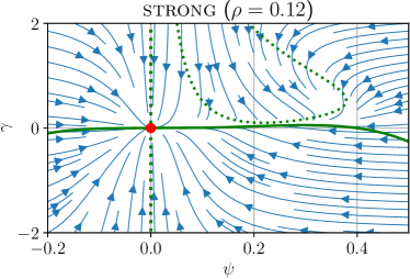
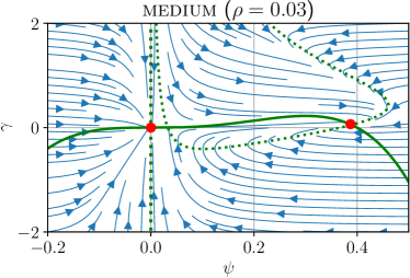
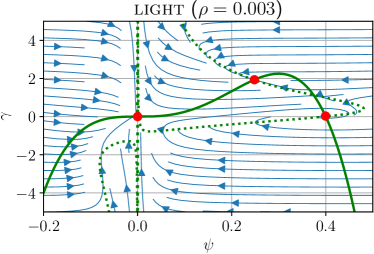
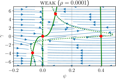
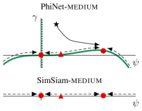
The state space diagrams of dynamics (1) are shown in Figure 2. In this figure, the nullclines $\dot{\psi}=0$ and $\dot{\gamma}=0$ are shown in the green real and dotted lines, respectively. Noting that intersecting points of nullclines are equilibrium points [20], we observe saddle-node bifurcation of PhiNet dynamics parametrized by weight decay $\rho>0$.

  • strong: Weight decay $\rho$ is too strong that the collapsed point $(\psi,\gamma)=(0,0)$ is a unique sink.

  • medium: A new sink $(\psi,\gamma)$ such that $\psi\gg 0$ and $\gamma\approx 0$ emerges. The number of sinks is two.

  • light: Another non-trivial sink $(\psi,\gamma)$ such that $\psi,\gamma\gg 0$ emerges. There are three sinks.

  • weak: The last sink emerges such that $\psi<0$ and $\gamma\ll 0$. The number of sinks is four.

Comparison with SimSiam dynamics.

Refer to caption
Figure 3: Illustration of SimSiam dynamics (2). Unlike the bivariate PhiNet dynamics shown in Figure 2, SimSiam dynamics is univariate, shown in the $\psi$-axis. The red dots are sinks.
Refer to caption
Figure 4: The SimSiam-medium flow is conjugate with the flow on the nullcline $\dot{\psi}=0$ (green real line) in PhiNet-medium.

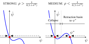
Tian et al. [46] derived the SimSiam dynamics under the same setup as above. Specifically, they modelled the encoder $f$ and the predictor $h$ with linear networks ${\mathbf{W}}_{f}{\bm{x}}$ and ${\mathbf{W}}_{h}{\bm{z}}$, respectively, and defined the gradient flow dynamics with the MSE loss $\|{\mathbf{W}}_{h}{\mathbf{W}}_{f}{\bm{x}}^{(1)}-{\textnormal{SG}}({\mathbf{W}}_{f}{\bm{x}}^{(2)})\|^{2}$ (without the additional predictor $g$). By decoupling the matrix dynamics into the eigenvalues with the same adiabatic elimination $\phi=\psi^{2}$, we can derive the SimSiam dynamics solely with respect to $\psi$-dynamics as follows:

$$\text{(SimSiam-dynamics)}\qquad\dot{\psi}=\{1-(1+\sigma^{2})\psi\}\psi^{2}-\rho\psi.$$ (2)

We set $\tau=1$ (ablating the exponential moving average used in BYOL) in Tian et al. [46, Eq. (16)] to obtain this dynamics. SimSiam is free from the additional predictor $g$, so the dynamics (2) is univariate, unlike the bivariate system (1). Figure 4 shows the dynamics (2).

The SimSiam dynamics bifurcates into strong and medium at $\rho=1/4(1+\sigma^{2})$. These two modes correspond to strong and medium of PhiNet in that $\psi$-axis of Figure 4 and the nullcline $\dot{\psi}=0$ (green real line) in Figure 2 are topologically conjugate. The other light and weak are peculiar to the PhiNet dynamics. By comparing Figures 2 and 4, we have the following observations:

  1. (C1)

    The retraction basin to non-collapsed solutions is wider: Since SimSiam dynamics is univariate, $\psi$ cannot avoid collapse once $\psi(0)$ is initialized outside the retraction basin to the non-collapse point $\psi^{*}\neq 0$ (namely, smaller than the source point $\blacktriangle$ in Figure 4). By contrast, PhiNet avoids collapse even if $\psi(0)$ is close to zero, as long as $\gamma(0)$ is sufficiently large (see the initial point $\bigstar$ in Figure 4).

  2. (C2)

    Even negative initialization $\psi$ can avoid collapse: In SimSiam-medium, $\psi$ cannot be attracted to the non-collapsed solution if $\psi(0)$ is initialized to negative. By contrast, PhiNet-weak has a negative sink (at the bottom left in Figure 2), which attracts negative initialization $\psi(0)<0$.

To sum it up, we have witnessed with a toy model that PhiNet is advantageous over SimSiam because the collapsed solution can be avoided more easily. This is why another predictor $g$ is beneficial.

Remark 1.

The learning dynamics analysis in this section reveals that smaller weight decay $\rho$ brings us benefits only regarding the stability of non-collapsed solutions. Indeed, we may benefit from larger $\rho$ to accelerate convergence to the invariant parabola and eigenspace alignment of $({\bm{\Phi}},{\mathbf{W}}_{h},{\mathbf{W}}_{g})$ (Appendices C.4 and C.2), each of which corresponds to the positive effects #3 and #7 in Tian et al. [46], respectively. Moreover, moderately large $\rho$ often yields good generalization in non-contrastive learning [7]. Thus, smaller $\rho$ may not be a silver bullet.

5 Experiments

We first test the robustness of PhiNets against the design choice and weight decay hyperparameter. We then discuss the effectiveness of X-PhiNets in online and continual learning.

5.1 Linear Probing Analysis

Refer to caption
Figure 5: PhiNet and X-PhiNet are robust against weight decay. We compared PhiNet variants in (a1)-(a2) and compared the existing non-contrastive methods with PhiNet in (b1)-(b2) on CIFAR10. We evaluated the performance using linear probing on the head. The loss function in brackets represents neocortex loss $L_{\textnormal{NC}}({\bm{\theta}})$. PhiNets perform particularly better than the baselines when weight decay is small.
Table 1: PhiNet is comparable to SimSiam. We trained the models for 100 epochs and then validated them on the test sets using linear probing on the head. We trained with three seeds and calculated means and variances (subscripts). Both are unstable when the weight decay is small, but PhiNet still achieves high accuracy.
Accuracy by Linear Probing (w.r.t. weight decay)
0.0 0.00001 0.00002 0.00005 0.0001 0.0002
SimSiam $25.41_{0.02}$ $2.63_{0.18}$ $60.82_{1.57}$ $44.51_{33.64}$ $68.17_{0.18}$ $67.12_{0.13}$
PhiNet (MSE) $49.89_{0.35}$ $55.90_{1.57}$ $33.92_{7.42}$ $66.73_{0.03}$ $68.25_{0.21}$ $67.83_{0.15}$

Figure 5 and Table 1 show the sensitivity analysis using CIFAR10 [22] and ImageNet [23], respectively, by changing the weight decay parameter. First, we emphasise the improvement of PhiNet over SimSiam for most of the setups, corroborating the success of the CLS-based modelling. Subsequently, we closely look at the results.

PhiNet-MSE improves SimSiam.

We observed weight decay significantly impacts the final model performance. When the MSE loss is used for Sim-2, PhiNet consistently outperforms the original SimSiam in all scenarios, shown in Figure 5 (right). Conversely, Figure 5 (left) and Table 9 in the appendix shows that PhiNet with the cosine loss (used for Sim-2) exhibits superior performance with lower weight decay but some degradation with higher weight decay values.

Bless of additional predictor.

To see whether the additional predictor $g$ besides $h$ is beneficial, we test variants of predictor $g$: $g=h$ (reminiscent of the recurrent structure in CA3) and $g={\mathbf{I}}$ (identity predictor). For CIFAR10 with batch size = 128, Figure 5 (left) indicates that the predictor choice slightly affects the final model performance if we properly set the weight decay. However, if we set the batch size as 1024, the separate predictor performs more stably over other choices.

Sim-2 loss should be MSE.

Based on Figure 5 and Table 11 in the appendix, we found that the MSE loss used for Sim-2 generally improves model performance across most weight decay parameters, while the negative cosine loss performs comparably to the MSE loss with smaller weight decay but degrades it with larger weight decay.

Overall, our sensitivity study on CIFAR10 revealed that PhiNets are robust to the choice of the weight decay parameter. See Appendix F.1 for more detailed sensitivity studies. In addition, the results for different batch sizes and datasets (STL10 [13]) can be found in Appendix F.3.

5.2 Online Learning and Continual Learning

Table 2: X-PhiNet performs good results when memorization is important. We trained PhiNets on CIFAR-5m and Split CIFAR-5m. In Split CIFAR-5m, Acc is the average of the final accuracy (higher is better), and Fg is Forgetting (smaller is better). We present the results for two different weight decay (5e-4 and 2e-5) in Split CIFAR-5m.
BYOL SimSiam Barlow PhiNet RM- X-PhiNet X-PhiNet
Twins (MSE) SimSiam (MSE) (Cos)
CIFAR-5m $81.05_{0.04}$ $77.71_{1.97}$ $85.32_{0.10}$ $76.74_{1.82}$ $82.09_{0.22}$ $87.30_{0.13}$ ${\bf 87.46_{0.14}}$
Split C-5m Acc $90.44_{0.28}$ $90.84_{0.31}$ $90.30_{0.17}$ $90.69_{0.11}$ $90.04_{0.11}$ $91.02_{0.36}$ ${\bf 92.83_{0.12}}$
(wd=5e-4) Fg $1.61_{0.50}$ $2.45_{0.42}$ $3.36_{1.10}$ $2.96_{0.23}$ $2.44_{0.22}$ $3.44_{0.36}$ $1.95_{0.19}$
Split C-5m Acc $86.87_{0.12}$ $88.20_{0.35}$ $89.86_{0.34}$ $88.60_{0.15}$ $87.07_{0.36}$ ${\bf 90.90_{0.38}}$ ${\bf 90.72_{0.23}}$
(wd=2e-5) Fg $-0.16_{0.23}$ $0.36_{0.51}$ $1.29_{0.94}$ $0.05_{0.19}$ $0.82_{0.14}$ $-1.03_{0.41}$ $0.43_{0.17}$
Refer to caption
Figure 6: X-PhiNet is also robust to weight decay in continual learning. We measured the mean accuracy and forgetting at different weight decay on Split CIFAR-5m.

SimSiam and other non-contrastive methods typically require up to $800$ epochs of training on CIFAR10, which is quite different from the online nature of brains. To address this, we conducted experiments using the CIFAR-5m dataset, which has six million synthetic CIFAR-10-like images generated by DDPM generative model [33]. Instead of training CIFAR10 with 50k samples for $800$ epochs, we trained CIFAR-5m with 5m samples for $8$ epochs. Although this is not exactly online learning, it seems closer to online learning compared to CIFAR10 due to the restriction on the training epochs. Table 2 shows that X-PhiNet has higher accuracy than SimSiam and PhiNet. The superior performance of X-PhiNet compared to PhiNet suggests that long-term memory with EMA is important in online learning. Sensitivity to weight decay and results for one-epoch online learning are given in Appendix E.1.

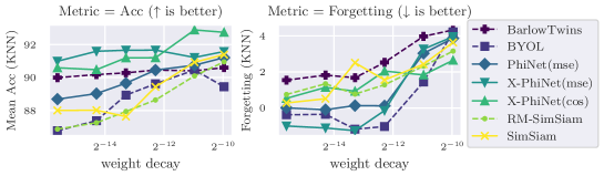
X-PhiNet is based on CLS theory, which explains continual learning in human brains. To evaluate the effectiveness of X-PhiNet in continual learning, we created a split CIFAR-5m dataset from CIFAR-5m, dividing it into five tasks, each with two classes. We trained on each task for one epoch and evaluated performance by the average accuracy across all tasks and the average forgetting, which is the difference between the peak accuracy and the final accuracy of each task. Table 2 shows that X-PhiNet has higher performance than SimSiam while maintaining minimal forgetting. Figure 6 further demonstrates that X-PhiNet consistently outperforms other methods like SimSiam in continual learning, regardless of weight decay. X-PhiNet also demonstrates high performance on Split CIFAR10 and Split CIFAR100, as well as when using replay methods (Appendix E.2).

6 Conclusion

In this paper, we proposed PhiNets based on non-contrastive learning with the temporal prediction hypothesis. Specifically, we leveraged StopGradient to artificially simulate the temporal difference, and the prediction errors are modelled via Sim-1 and Sim-2 losses. Through theoretical analysis of learning dynamics, we showed that the proposed PhiNets have an advantage over SimSiam by more easily avoiding collapsed solutions. We empirically validated that the proposed PhiNets are robust with respect to weight decay and favorably comparable with SimSiam in terms of final classification performance. Experimental results also show that X-PhiNet performs better than SimSiam in online and continual learning, where memory function matters.

Acknowledgement

The authors thank Kenji Doya and Tomoki Fukaki for their helpful comments. We also thank Rio Yokota for probiding computational resources. M.Y. and H.B. were supported by MEXT KAKENHI Grant Number 24K03004 and Y.T. was supported by KAKENHI Grant Number 23KJ1336.

References

  • Alonso et al. [2022] N. Alonso, B. Millidge, J. Krichmar, and E. O. Neftci. A theoretical framework for inference learning. NeurIPS, 2022.
  • Arani et al. [2022] E. Arani, F. Sarfraz, and B. Zonooz. Learning fast, learning slow: A general continual learning method based on complementary learning system. In ICLR, 2022.
  • Awasthi et al. [2022] P. Awasthi, N. Dikkala, and P. Kamath. Do more negative samples necessarily hurt in contrastive learning? In ICML, 2022.
  • Bao [2023] H. Bao. Feature normalization prevents collapse of non-contrastive learning dynamics. arXiv preprint arXiv:2309.16109, 2023.
  • Bao et al. [2022] H. Bao, Y. Nagano, and K. Nozawa. On the surrogate gap between contrastive and supervised losses. In ICML, 2022.
  • Becker and Hinton [1992] S. Becker and G. E. Hinton. Self-organizing neural network that discovers surfaces in random-dot stereograms. Nature, 355(6356):161–163, 1992.
  • Cabannes et al. [2023] V. Cabannes, B. Kiani, R. Balestriero, Y. LeCun, and A. Bietti. The SSL interplay: Augmentations, inductive bias, and generalization. In ICML, 2023.
  • Caron et al. [2020] M. Caron, I. Misra, J. Mairal, P. Goyal, P. Bojanowski, and A. Joulin. Unsupervised learning of visual features by contrasting cluster assignments. NeurIPS, 2020.
  • Caron et al. [2021] M. Caron, H. Touvron, I. Misra, H. Jégou, J. Mairal, P. Bojanowski, and A. Joulin. Emerging properties in self-supervised vision transformers. In ICCV, 2021.
  • Chen et al. [2020] T. Chen, S. Kornblith, M. Norouzi, and G. Hinton. A simple framework for contrastive learning of visual representations. In ICML, 2020.
  • Chen and He [2021] X. Chen and K. He. Exploring simple Siamese representation learning. In CVPR, 2021.
  • Chen et al. [2022] Y. Chen, H. Zhang, M. Cameron, and T. Sejnowski. Predictive sequence learning in the hippocampal formation. bioRxiv, pages 2022–05, 2022.
  • Coates et al. [2011] A. Coates, A. Ng, and H. Lee. An analysis of single-layer networks in unsupervised feature learning. In AISTATS, 2011.
  • Friston [2005] K. Friston. A theory of cortical responses. Philosophical Transactions of the Royal Society B: Biological Sciences, 360(1456):815–836, 2005.
  • Fu et al. [2024] F. Fu, Y. Gao, Z. Lu, H. Wu, and S. Zhao. Unsupervised continual learning of image representation via rememory-based simsiam. In ICASSP, 2024.
  • Grill et al. [2020] J.-B. Grill, F. Strub, F. Altché, C. Tallec, P. Richemond, E. Buchatskaya, C. Doersch, B. Avila Pires, Z. Guo, M. Gheshlaghi Azar, et al. Bootstrap your own latent-a new approach to self-supervised learning. NeurIPS, 2020.
  • Halvagal et al. [2023] M. S. Halvagal, A. Laborieux, and F. Zenke. Implicit variance regularization in non-contrastive SSL. NeurIPS, 2023.
  • Han et al. [2018] K. Han, H. Wen, Y. Zhang, D. Fu, E. Culurciello, and Z. Liu. Deep predictive coding network with local recurrent processing for object recognition. NeurIPS, 2018.
  • Henaff [2020] O. Henaff. Data-efficient image recognition with contrastive predictive coding. In ICML, 2020.
  • Hirsch et al. [2012] M. W. Hirsch, S. Smale, and R. L. Devaney. Differential Equations, Dynamical Systems, and an Introduction to Chaos. Academic Press, 2012.
  • Hsu et al. [2018] Y.-C. Hsu, Y.-C. Liu, A. Ramasamy, and Z. Kira. Re-evaluating continual learning scenarios: A categorization and case for strong baselines. arXiv preprint arXiv:1810.12488, 2018.
  • Krizhevsky [2009] A. Krizhevsky. Learning multiple layers of features from tiny images. 2009.
  • Krizhevsky et al. [2012] A. Krizhevsky, I. Sutskever, and G. E. Hinton. Imagenet classification with deep convolutional neural networks. In NIPS, 2012.
  • Kumaran et al. [2016] D. Kumaran, D. Hassabis, and J. L. McClelland. What learning systems do intelligent agents need? complementary learning systems theory updated. Trends in Cognitive Sciences, 20:512–534, 2016.
  • Lin et al. [2022] Z. Lin, Y. Wang, and H. Lin. Continual contrastive learning for image classification. In ICME, 2022.
  • Lindsay [2021] G. W. Lindsay. Convolutional neural networks as a model of the visual system: Past, present, and future. Journal of Cognitive Neuroscience, 33(10):2017–2031, 2021.
  • Liu et al. [2022] H. Liu, J. Z. HaoChen, A. Gaidon, and T. Ma. Self-supervised learning is more robust to dataset imbalance. In ICLR, 2022.
  • Liu et al. [2023] Z. Liu, E. S. Lubana, M. Ueda, and H. Tanaka. What shapes the loss landscape of self supervised learning? In ICLR, 2023.
  • Madaan et al. [2022] D. Madaan, J. Yoon, Y. Li, Y. Liu, and S. J. Hwang. Representational continuity for unsupervised continual learning. In ICLR, 2022.
  • McClelland et al. [1995] J. L. McClelland, B. L. McNaughton, and R. C. O’Reilly. Why there are complementary learning systems in the hippocampus and neocortex: insights from the successes and failures of connectionist models of learning and memory. Psychological Review, 102(3):419, 1995.
  • Millidge et al. [2023] B. Millidge, Y. Song, T. Salvatori, T. Lukasiewicz, and R. Bogacz. Backpropagation at the infinitesimal inference limit of energy-based models: Unifying predictive coding, equilibrium propagation, and contrastive Hebbian learning. In ICLR, 2023.
  • Mumford [1992] D. Mumford. On the computational architecture of the neocortex: II the role of cortico-cortical loops. Biological Cybernetics, 66(3):241–251, 1992.
  • Nakkiran et al. [2021] P. Nakkiran, B. Neyshabur, and H. Sedghi. The deep bootstrap framework: Good online learners are good offline generalizers. In ICLR, 2021.
  • Oord et al. [2018] A. v. d. Oord, Y. Li, and O. Vinyals. Representation learning with contrastive predictive coding. arXiv preprint arXiv:1807.03748, 2018.
  • Pham et al. [2021a] Q. Pham, C. Liu, and S. Hoi. DualNet: Continual learning, fast and slow. NeurIPS, 2021a.
  • Pham et al. [2021b] Q. Pham, C. Liu, D. Sahoo, and S. Hoi. Contextual transformation networks for online continual learning. In ICLR, 2021b.
  • Pham et al. [2023a] Q. Pham, C. Liu, and S. C. Hoi. Continual learning, fast and slow. IEEE Transactions on Pattern Analysis and Machine Intelligence, 2023a.
  • Pham et al. [2023b] Q. Pham, C. Liu, D. Sahoo, and S. Hoi. Learning fast and slow for online time series forecasting. In ICLR, 2023b.
  • Ramsauer et al. [2020] H. Ramsauer, B. Schäfl, J. Lehner, P. Seidl, M. Widrich, L. Gruber, M. Holzleitner, M. Pavlovic, G. K. Sandve, V. Greiff, D. P. Kreil, M. Kopp, G. Klambauer, J. Brandstetter, and S. Hochreiter. Hopfield networks is all you need. arXiv preprint arXiv:2008.02217, 2020.
  • Rao and Ballard [1999] R. P. Rao and D. H. Ballard. Predictive coding in the visual cortex: a functional interpretation of some extra-classical receptive-field effects. Nature Neuroscience, 2(1):79–87, 1999.
  • Russakovsky et al. [2015] O. Russakovsky, J. Deng, H. Su, J. Krause, S. Satheesh, S. Ma, Z. Huang, A. Karpathy, A. Khosla, M. Bernstein, et al. Imagenet large scale visual recognition challenge. International Journal of Computer Vision, 115:211–252, 2015.
  • Sarnthein et al. [2023] F. Sarnthein, G. Bachmann, S. Anagnostidis, and T. Hofmann. Random teachers are good teachers. In ICML. PMLR, 2023.
  • Smith et al. [2021] J. Smith, C. Taylor, S. Baer, and C. Dovrolis. Unsupervised progressive learning and the STAM architecture. In IJCAI, 2021.
  • Srinivasan et al. [1982] M. V. Srinivasan, S. B. Laughlin, and A. Dubs. Predictive coding: a fresh view of inhibition in the retina. Proceedings of the Royal Society of London. Series B. Biological Sciences, 216(1205):427–459, 1982.
  • Tang et al. [2023] Y. Tang, Z. D. Guo, P. H. Richemond, B. A. Pires, Y. Chandak, R. Munos, M. Rowland, M. G. Azar, C. Le Lan, C. Lyle, et al. Understanding self-predictive learning for reinforcement learning. In ICML, 2023.
  • Tian et al. [2021] Y. Tian, X. Chen, and S. Ganguli. Understanding self-supervised learning dynamics without contrastive pairs. In ICML, 2021.
  • Van de Ven et al. [2020] G. M. Van de Ven, H. T. Siegelmann, and A. S. Tolias. Brain-inspired replay for continual learning with artificial neural networks. Nature communications, 2020.
  • Vyas et al. [2023] N. Vyas, A. Atanasov, B. Bordelon, D. Morwani, S. Sainathan, and C. Pehlevan. Feature-learning networks are consistent across widths at realistic scales. In NeurIPS, 2023.
  • Wen et al. [2018] H. Wen, J. Shi, W. Chen, and Z. Liu. Deep residual network predicts cortical representation and organization of visual features for rapid categorization. Scientific Reports, 8(1):3752, 2018.

Appendix A Limitations and Future Work

One major limitation of our approach is the use of backpropagation, which differs from the mechanisms in biological neural networks. Our long-term goal is to eliminate backpropagation to better imitate brain function, but this work focuses on the model’s structural aspects. Currently, backpropagation-free predictive coding mechanisms for complex architectures like ResNet are in the early stages of development, with most research limited to simple CNNs. Conversely, non-contrastive methods like SimSiam require more advanced models than ResNet. Future research should explore if the proposed structure can enable effective learning with backpropagation-free predictive coding. Another key difference between PhiNet and brains is the presence of recurrent structures. However, in this PhiNet, only one time step is considered, so it is possible that the recurrent structure required to predict time series data was not necessary. Making the data into time series data and adding a recurrent structure to the model remains as future work.

It is also unclear whether cosine loss or MSE loss is more suitable for the sim-2 in PhiNets. Cosine loss performs better when weight decay is small or online and continual learning where the additional predictor of PhiNets is important. However, MSE loss is preferable when weight decay is large on CIFAR10. This is likely because using cosine loss in sim-2 has a stronger impact on learning dynamics compared to MSE loss. Analyzing gradient norms could be useful for this kind of evaluation, but is left for future work.

Appendix B Broader Impacts

Learning representations is a challenging task, and most approaches are ML-based. In contrast, this work incorporates the structure of the human hippocampus to find better representations in a self-supervised manner and proposes an architecture with stable behavior. Since the PhiNet model resembles the modern understanding of hippocampal structure under temporal prediction hypotheses, it can potentially integrate new findings from neuroscience. Therefore, our paper will have an impact on both machine learning and neuroscience.

Appendix C Details of Learning Dynamics Analysis

In this section, we complement the missing details of learning dynamics analysis provided in Section 4.

C.1 Derivation of Matrix Dynamics

Recall the PhiNet loss function:

$$\overline{L}\coloneqq\frac{1}{2}\mathbb{E}_{{\bm{x}}}\mathbb{E}_{{\bm{x}}^{(1)},{\bm{x}}^{(2)}|{\bm{x}}}\left[\|{\mathbf{W}}_{h}{\mathbf{W}}_{f}{\bm{x}}^{(1)}-{\textnormal{SG}}({\mathbf{W}}_{f}{\mathbf{x}}^{(2)})\|^{2}+\|{\mathbf{W}}_{g}{\mathbf{W}}_{h}{\mathbf{W}}_{f}{\bm{x}}^{(1)}-{\textnormal{SG}}({\mathbf{W}}_{f}{\bm{x}})\|^{2}\right].$$

Let us derive its matrix gradient.

$\displaystyle\nabla_{{\mathbf{W}}_{f}}\overline{L}$ $\displaystyle=\frac{1}{2}\nabla_{{\mathbf{W}}_{f}}\mathbb{E}\left[({\bm{x}}^{(1)\top}{\mathbf{W}}_{f}^{\top}{\mathbf{W}}_{h}^{\top}-{\textnormal{SG}}({\bm{x}}^{(2)\top}{\mathbf{W}}_{f}^{\top}))({\mathbf{W}}_{h}{\mathbf{W}}_{f}{\bm{x}}^{(1)}-{\textnormal{SG}}({\mathbf{W}}_{f}{\mathbf{x}}^{(2)}))\right.$
$\displaystyle\phantom{=\frac{1}{2}\nabla_{{\mathbf{W}}_{f}}\mathbb{E}~{}~{}}\left.+({\bm{x}}^{(1)}{\mathbf{W}}_{f}^{\top}{\mathbf{W}}_{h}^{\top}{\mathbf{W}}_{g}^{\top}-{\textnormal{SG}}({\bm{x}}^{\top}{\mathbf{W}}_{f}^{\top}))({\mathbf{W}}_{g}{\mathbf{W}}_{h}{\mathbf{W}}_{f}{\bm{x}}^{(1)}-{\textnormal{SG}}({\mathbf{W}}_{f}{\bm{x}}))\right]$
$\displaystyle=\left\{{\mathbf{W}}_{h}^{\top}{\mathbf{W}}_{h}{\mathbf{W}}_{f}\mathbb{E}[{\bm{x}}^{(1)}{\bm{x}}^{(1)\top}]-{\mathbf{W}}_{h}^{\top}{\mathbf{W}}_{f}\mathbb{E}[{\bm{x}}^{(2)}{\bm{x}}^{(1)\top}]\right\}$
$\displaystyle\phantom{=~{}~{}}+\left\{{\mathbf{W}}_{h}^{\top}{\mathbf{W}}_{g}^{\top}{\mathbf{W}}_{g}{\mathbf{W}}_{h}{\mathbf{W}}_{f}\mathbb{E}[{\bm{x}}^{(1)}{\bm{x}}^{(1)\top}]-{\mathbf{W}}_{h}^{\top}{\mathbf{W}}_{g}^{\top}{\mathbf{W}}_{f}\mathbb{E}[{\bm{x}}{\bm{x}}^{(1)\top}]\right\}$
$\displaystyle={\mathbf{W}}_{h}^{\top}\left\{({\mathbf{I}}+{\mathbf{W}}_{g}^{\top}{\mathbf{W}}_{g}){\mathbf{W}}_{h}{\mathbf{W}}_{f}\mathbb{E}[{\bm{x}}^{(1)}{\bm{x}}^{(1)\top}]-{\mathbf{W}}_{f}\mathbb{E}[{\bm{x}}^{(2)}{\bm{x}}^{(1)\top}]-{\mathbf{W}}_{g}^{\top}{\mathbf{W}}_{f}\mathbb{E}[{\bm{x}}{\bm{x}}^{(1)\top}]\right\}$
$\displaystyle={\mathbf{W}}_{h}^{\top}\left\{(1+\sigma^{2})({\mathbf{I}}+{\mathbf{W}}_{g}^{\top}{\mathbf{W}}_{g}){\mathbf{W}}_{h}-({\mathbf{I}}+{\mathbf{W}}_{g}^{\top})\right\}{\mathbf{W}}_{f},$

where the last line is derived from our assumption on the data distributions:

$\displaystyle\mathbb{E}_{{\bm{x}}}\mathbb{E}_{{\bm{x}}^{(1)}|{\bm{x}}}[{\bm{x}}^{(1)}{\bm{x}}^{(1)\top}]$ $\displaystyle=\mathbb{E}_{{\bm{x}}}[{\bm{x}}{\bm{x}}^{\top}]+\sigma^{2}{\mathbf{I}}=(1+\sigma^{2}){\mathbf{I}},$
$\displaystyle\mathbb{E}_{{\bm{x}}}\mathbb{E}_{{\bm{x}}^{(1)},{\bm{x}}^{(2)}|{\bm{x}}}[{\bm{x}}^{(2)}{\bm{x}}^{(1)\top}]$ $\displaystyle=\mathbb{E}_{{\bm{x}}}[{\bm{x}}{\bm{x}}^{\top}]={\mathbf{I}},$
$\displaystyle\mathbb{E}_{{\bm{x}}}\mathbb{E}_{{\bm{x}}^{(1)}|{\bm{x}}}[{\bm{x}}{\bm{x}}^{(1)\top}]$ $\displaystyle=\mathbb{E}_{{\bm{x}}}[{\bm{x}}{\bm{x}}^{\top}]={\mathbf{I}}.$

Similarly, we derive $\nabla_{{\mathbf{W}}_{g}}\overline{L}$ and $\nabla_{{\mathbf{W}}_{h}}\overline{L}$.

$\displaystyle\nabla_{{\mathbf{W}}_{g}}\overline{L}$ $\displaystyle={\mathbf{W}}_{h}{\mathbf{W}}_{f}\mathbb{E}[{\bm{x}}^{(1)}{\bm{x}}^{(1)\top}]{\mathbf{W}}_{f}^{\top}{\mathbf{W}}_{h}^{\top}-{\mathbf{W}}_{f}\mathbb{E}[{\bm{x}}{\bm{x}}^{(1)\top}]{\mathbf{W}}_{f}^{\top}{\mathbf{W}}_{h}^{\top}$
$\displaystyle=\left\{(1+\sigma^{2}){\mathbf{W}}_{h}-{\mathbf{I}}\right\}{\mathbf{W}}_{f}{\mathbf{W}}_{f}^{\top}{\mathbf{W}}_{h}^{\top}.$
$\displaystyle\nabla_{{\mathbf{W}}_{h}}\overline{L}$ $\displaystyle=\left\{{\mathbf{W}}_{h}{\mathbf{W}}_{f}\mathbb{E}[{\bm{x}}^{(1)}{\bm{x}}^{(1)\top}]{\mathbf{W}}_{f}^{\top}-{\mathbf{W}}_{f}\mathbb{E}[{\bm{x}}^{(2)}{\bm{x}}^{(1)\top}]{\mathbf{W}}_{f}^{\top}\right\}$
$\displaystyle\phantom{=~{}~{}}+\left\{{\mathbf{W}}_{g}^{\top}{\mathbf{W}}_{g}{\mathbf{W}}_{h}{\mathbf{W}}_{f}\mathbb{E}[{\bm{x}}^{(1)}{\bm{x}}^{(1)\top}]{\mathbf{W}}_{f}^{\top}-{\mathbf{W}}_{g}^{\top}{\mathbf{W}}_{f}\mathbb{E}[{\bm{x}}{\bm{x}}^{(1)\top}]{\mathbf{W}}_{f}^{\top}\right\}$
$\displaystyle=\left\{(1+\sigma^{2})({\mathbf{I}}+{\mathbf{W}}_{g}^{\top}{\mathbf{W}}_{g}){\mathbf{W}}_{h}-({\mathbf{I}}+{\mathbf{W}}_{g}^{\top})\right\}{\mathbf{W}}_{f}{\mathbf{W}}_{f}^{\top}.$

From these, we obtain the matrix dynamics.

C.2 Eigenspace Alignment

Our aim is to show that the three matrices ${\bm{\Phi}}$, ${\mathbf{W}}_{g}$, and ${\mathbf{W}}_{h}$ share a common eigenspace, i.e., simultaneously diagonalizable, asymptotically in time $t$. Let

$${\mathbf{C}}_{1}\coloneqq{[{{\bm{\Phi}}},{{\mathbf{W}}_{g}}]},\quad{\mathbf{C}}_{2}\coloneqq{[{{\bm{\Phi}}},{{\mathbf{W}}_{h}}]},\quad\text{and}\quad{\mathbf{C}}_{3}\coloneqq{[{{\mathbf{W}}_{g}},{{\mathbf{W}}_{h}}]},$$

where ${[{{\mathbf{A}}},{{\mathbf{B}}}]}\coloneqq{\mathbf{A}}{\mathbf{B}}-{\mathbf{B}}{\mathbf{A}}$ is the commutator (matrix). By noting that commutative matrices are simultaneously diagonalizable, we show that the time-dependent commutators ${\mathbf{C}}_{1}(t)$, ${\mathbf{C}}_{2}(t)$, and ${\mathbf{C}}_{3}(t)$ asymptotically converges to ${\mathbf{O}}$ as $t\to\infty$.

Hereafter, we assume the symmetry assumption (A1) on ${\mathbf{W}}_{g}$ and ${\mathbf{W}}_{h}$, and heavily use the following formulas on commutators implicitly:

  • $[{\mathbf{A}},{\mathbf{A}}]={\mathbf{O}}$.

  • $[{\mathbf{A}},{\mathbf{B}}]=-[{\mathbf{B}},{\mathbf{A}}]$.

  • $[{\mathbf{A}},{\mathbf{B}}{\mathbf{C}}]=[{\mathbf{A}},{\mathbf{B}}]{\mathbf{C}}+{\mathbf{B}}[{\mathbf{A}},{\mathbf{C}}]$.

  • $[{\mathbf{A}}{\mathbf{B}},{\mathbf{C}}]={\mathbf{A}}[{\mathbf{B}},{\mathbf{C}}]+[{\mathbf{A}},{\mathbf{C}}]{\mathbf{B}}$.

First, compute $\dot{\mathbf{C}}_{1}$ based on the matrix dynamics of ${\bm{\Phi}}$ (can be found in Appendix C.3) and ${\mathbf{W}}_{g}$:

$\displaystyle\dot{\mathbf{C}}_{1}$ $\displaystyle=\dot{\bm{\Phi}}{\mathbf{W}}_{g}+{\bm{\Phi}}\dot{\mathbf{W}}_{g}-\dot{\mathbf{W}}_{g}{\bm{\Phi}}-{\mathbf{W}}_{g}\dot{\bm{\Phi}}$
$\displaystyle=\{-(1+\sigma^{2})({\mathbf{W}}_{h}({\mathbf{I}}+{\mathbf{W}}_{g}^{2}){\mathbf{W}}_{h}{\bm{\Phi}}+{\bm{\Phi}}{\mathbf{W}}_{h}({\mathbf{I}}+{\mathbf{W}}_{g}^{2}){\mathbf{W}}_{h})+({\mathbf{W}}_{h}{\bm{\Phi}}+{\bm{\Phi}}{\mathbf{W}}_{h})$
$\displaystyle\phantom{=}\;\;+({\mathbf{W}}_{h}{\mathbf{W}}_{g}{\bm{\Phi}}+{\bm{\Phi}}{\mathbf{W}}_{g}{\mathbf{W}}_{h})-2\rho{\bm{\Phi}}\}{\mathbf{W}}_{g}+{\bm{\Phi}}\{-((1+\sigma^{2}){\mathbf{W}}_{h}-{\mathbf{I}}){\bm{\Phi}}{\mathbf{W}}_{h}-\rho{\mathbf{W}}_{g}\}$
$\displaystyle\phantom{=}+\{((1+\sigma^{2}){\mathbf{W}}_{h}-{\mathbf{I}}){\bm{\Phi}}{\mathbf{W}}_{h}+\rho{\mathbf{W}}_{g}\}{\bm{\Phi}}$
$\displaystyle\phantom{=}+{\mathbf{W}}_{g}\{(1+\sigma^{2})({\mathbf{W}}_{h}({\mathbf{I}}+{\mathbf{W}}_{g}^{2}){\mathbf{W}}_{h}{\bm{\Phi}}+{\bm{\Phi}}{\mathbf{W}}_{h}({\mathbf{I}}+{\mathbf{W}}_{g}^{2}){\mathbf{W}}_{h})-({\mathbf{W}}_{h}{\bm{\Phi}}+{\bm{\Phi}}{\mathbf{W}}_{h})$
$\displaystyle\phantom{=}\;\;-({\mathbf{W}}_{h}{\mathbf{W}}_{g}{\bm{\Phi}}+{\bm{\Phi}}{\mathbf{W}}_{g}{\mathbf{W}}_{h})+2\rho{\bm{\Phi}}\}$
$\displaystyle=-3\rho{\mathbf{C}}_{1}+(1+\sigma^{2}){[{{\mathbf{W}}_{g}},{{\mathbf{W}}_{h}({\mathbf{I}}+{\mathbf{W}}_{g}^{2}){\mathbf{W}}_{h}{\bm{\Phi}}}]}+(1+\sigma^{2}){[{{\mathbf{W}}_{g}},{{\bm{\Phi}}{\mathbf{W}}_{h}({\mathbf{I}}+{\mathbf{W}}_{g}^{2}){\mathbf{W}}_{h}}]}$
$\displaystyle\phantom{=}+{[{{\mathbf{W}}_{h}{\bm{\Phi}}+{\bm{\Phi}}{\mathbf{W}}_{h}},{{\mathbf{W}}_{g}}]}+{[{{\mathbf{W}}_{h}},{{\mathbf{W}}_{g}{\bm{\Phi}}{\mathbf{W}}_{g}}]}+{[{{\bm{\Phi}}},{{\mathbf{W}}_{g}{\mathbf{W}}_{h}{\mathbf{W}}_{g}}]}$
$\displaystyle\phantom{=}+{[{((1+\sigma^{2}){\mathbf{W}}_{h}-{\mathbf{I}}){\bm{\Phi}}{\mathbf{W}}_{h}},{{\bm{\Phi}}}]}$
$\displaystyle=-3\rho{\mathbf{C}}_{1}+(1+\sigma^{2})\{({\mathbf{C}}_{3}{\mathbf{W}}_{h}{\bm{\Phi}}+{\bm{\Phi}}{\mathbf{W}}_{h}{\mathbf{C}}_{3})+({\mathbf{W}}_{h}{\mathbf{C}}_{3}{\bm{\Phi}}+{\bm{\Phi}}{\mathbf{C}}_{3}{\mathbf{W}}_{h})$
$\displaystyle\phantom{=}\;\;+({\mathbf{C}}_{3}{\mathbf{W}}_{g}^{2}{\mathbf{W}}_{h}+{\mathbf{W}}_{h}{\mathbf{W}}_{g}^{2}{\mathbf{C}}_{3}){\bm{\Phi}}-({\mathbf{W}}_{h}{\mathbf{W}}_{g}^{2}{\mathbf{W}}_{h}{\mathbf{C}}_{1}+{\mathbf{C}}_{1}{\mathbf{W}}_{h}{\mathbf{W}}_{g}^{2}{\mathbf{W}}_{h})$
$\displaystyle\phantom{=}\;\;-({\mathbf{W}}_{h}^{2}{\mathbf{C}}_{1}+{\mathbf{C}}_{1}{\mathbf{W}}_{h}^{2})+{\bm{\Phi}}({\mathbf{C}}_{3}{\mathbf{W}}_{g}^{2}{\mathbf{W}}_{h}+{\mathbf{W}}_{h}{\mathbf{W}}_{g}^{2}{\mathbf{C}}_{3})\}$
$\displaystyle\phantom{=}+({\mathbf{W}}_{h}{\mathbf{C}}_{1}+{\mathbf{C}}_{1}{\mathbf{W}}_{h})-({\mathbf{C}}_{3}{\bm{\Phi}}+{\bm{\Phi}}{\mathbf{C}}_{3})-({\mathbf{C}}_{3}{\bm{\Phi}}{\mathbf{W}}_{g}+{\mathbf{W}}_{g}{\bm{\Phi}}{\mathbf{C}}_{3})$
$\displaystyle\phantom{=}+({\mathbf{C}}_{1}{\mathbf{W}}_{h}{\mathbf{W}}_{g}+{\mathbf{W}}_{g}{\mathbf{W}}_{h}{\mathbf{C}}_{1})-(1+\sigma^{2})({\mathbf{W}}_{h}{\bm{\Phi}}{\mathbf{C}}_{2}+{\mathbf{C}}_{2}{\bm{\Phi}}{\mathbf{W}}_{h})+{\bm{\Phi}}{\mathbf{C}}_{2}.$

Similarly, $\dot{\mathbf{C}}_{2}$ and $\dot{\mathbf{C}}_{3}$ are computed:

$\displaystyle\dot{\mathbf{C}}_{2}$ $\displaystyle=-3\rho{\mathbf{C}}_{2}+({\mathbf{C}}_{2}{\mathbf{W}}_{h}+{\mathbf{W}}_{h}{\mathbf{C}}_{2})-{\mathbf{C}}_{1}{\bm{\Phi}}+({\mathbf{W}}_{g}{\mathbf{C}}_{2}+{\mathbf{C}}_{2}{\mathbf{W}}_{g})+({\mathbf{C}}_{3}{\bm{\Phi}}+{\bm{\Phi}}{\mathbf{C}}_{3})$
$\displaystyle\phantom{=}-(1+\sigma^{2}){\mathbf{C}}_{2}{\bm{\Phi}}-(1+\sigma^{2})({\mathbf{W}}_{g}{\mathbf{C}}_{1}+{\mathbf{C}}_{1}{\mathbf{W}}_{g})+(1+\sigma^{2}){\mathbf{W}}_{h}({\mathbf{C}}_{3}{\mathbf{W}}_{g}+{\mathbf{W}}_{g}{\mathbf{C}}_{3})$
$\displaystyle\phantom{=}-(1+\sigma^{2})({\mathbf{W}}_{h}({\mathbf{I}}+{\mathbf{W}}_{g}^{2}){\mathbf{W}}_{h}{\mathbf{C}}_{2}+{\mathbf{C}}_{2}{\mathbf{W}}_{h}({\mathbf{I}}+{\mathbf{W}}_{g}^{2}){\mathbf{W}}_{h})$
$\displaystyle\phantom{=}+(1+\sigma^{2}){\bm{\Phi}}{\mathbf{W}}_{h}({\mathbf{C}}_{3}{\mathbf{W}}_{g}+{\mathbf{W}}_{g}{\mathbf{C}}_{3}){\mathbf{W}}_{h},$
$\displaystyle\dot{\mathbf{C}}_{3}$ $\displaystyle=-3\rho{\mathbf{C}}_{3}+({\mathbf{I}}-(1+\sigma^{2}){\mathbf{W}}_{h}){\mathbf{C}}_{2}{\mathbf{W}}_{h}+(1+\sigma^{2})({\mathbf{I}}+{\mathbf{W}}_{g}^{2})({\mathbf{W}}_{h}{\mathbf{C}}_{1}-{\mathbf{C}}_{3}{\bm{\Phi}})$
$\displaystyle\phantom{=}+({\mathbf{I}}+{\mathbf{W}}_{g}){\mathbf{C}}_{1}.$

Next, we vectorize the commutator matrices—for ${\mathbf{C}}\in\mathbb{R}^{h\times h}$, ${\mathrm{vec}({{\mathbf{C}}})}\in\mathbb{R}^{h^{2}}$ indicates a (column) vector stacking the columns of ${\mathbf{C}}$. For the commutators ${\mathbf{C}}_{1}$, ${\mathbf{C}}_{2}$, and ${\mathbf{C}}_{3}$, let us write ${\bm{\xi}}\coloneqq{\mathrm{vec}({{\mathbf{C}}_{1}})}$, ${\bm{\eta}}\coloneqq{\mathrm{vec}({{\mathbf{C}}_{2}})}$, and ${\bm{\zeta}}\coloneqq{\mathrm{vec}({{\mathbf{C}}_{3}})}$. In what follows, we heavily leverage the vectorization formula:

  • ${\mathrm{vec}({{\mathbf{A}}{\mathbf{B}}{\mathbf{C}}})}=({\mathbf{C}}^{\top}\otimes{\mathbf{A}}){\mathrm{vec}({{\mathbf{B}}})}=({\mathbf{I}}\otimes{\mathbf{A}}{\mathbf{B}}){\mathrm{vec}({{\mathbf{C}}})}=({\mathbf{C}}^{\top}{\mathbf{B}}^{\top}\otimes{\mathbf{I}}){\mathrm{vec}({{\mathbf{A}}})}$

  • ${\mathrm{vec}({{\mathbf{A}}{\mathbf{B}}})}=({\mathbf{I}}\otimes{\mathbf{A}}){\mathrm{vec}({{\mathbf{B}}})}=({\mathbf{B}}^{\top}\otimes{\mathbf{I}}){\mathrm{vec}({{\mathbf{A}}})}$

Here, ${\mathbf{A}}\otimes{\mathbf{B}}$ denotes the Kronecker product of two matrices. We write ${\mathbf{A}}\oplus{\mathbf{B}}\coloneqq{\mathbf{A}}\otimes{\mathbf{B}}+{\mathbf{B}}\otimes{\mathbf{A}}$ for notational convenience. We derive the ODE of ${\bm{\xi}}={\mathrm{vec}({{\mathbf{C}}_{1}})}$ as follows:

$\displaystyle\dot{\bm{\xi}}$ $\displaystyle=-3\rho{\mathbf{I}}{\bm{\xi}}+(1+\sigma^{2})(({\bm{\Phi}}{\mathbf{W}}_{h}\oplus{\mathbf{I}}){\bm{\zeta}}+({\bm{\Phi}}\oplus{\mathbf{W}}_{h}){\bm{\zeta}}+({\bm{\Phi}}\otimes{\mathbf{I}})({\mathbf{W}}_{h}{\mathbf{W}}_{g}^{2}\oplus{\mathbf{I}}){\bm{\zeta}}$
$\displaystyle\phantom{=}\;\;-({\mathbf{W}}_{h}{\mathbf{W}}_{g}^{2}{\mathbf{W}}_{h}\oplus{\mathbf{I}}){\bm{\xi}}-({\mathbf{I}}\oplus{\mathbf{W}}_{h}^{2}){\bm{\xi}}+({\mathbf{I}}\otimes{\bm{\Phi}})({\mathbf{W}}_{h}{\mathbf{W}}_{g}^{2}\oplus{\mathbf{I}}){\bm{\zeta}})+({\mathbf{I}}\oplus{\mathbf{W}}_{h}){\bm{\xi}}$
$\displaystyle\phantom{=}-({\bm{\Phi}}\oplus{\mathbf{I}}){\bm{\zeta}}-({\mathbf{W}}_{g}{\bm{\Phi}}\oplus{\mathbf{I}}){\bm{\zeta}}+({\mathbf{W}}_{g}{\mathbf{W}}_{h}\oplus{\mathbf{I}}){\bm{\xi}}-(1+\sigma^{2})({\mathbf{I}}\oplus{\mathbf{W}}_{h}{\bm{\Phi}}){\bm{\eta}}+({\mathbf{I}}\otimes{\bm{\Phi}}){\bm{\eta}}$
$\displaystyle=-\{3\rho{\mathbf{I}}+{\mathbf{I}}\oplus((1+\sigma^{2}){\mathbf{W}}_{h}({\mathbf{I}}+{\mathbf{W}}_{g}^{2}){\mathbf{W}}_{h})+{\mathbf{W}}_{h}({\mathbf{I}}+{\mathbf{W}}_{g})\}{\bm{\xi}}$
$\displaystyle\phantom{=}-\{(1+\sigma^{2})({\mathbf{I}}\otimes{\mathbf{W}}_{h}{\bm{\Phi}})-{\mathbf{I}}\otimes{\bm{\Phi}}\}{\bm{\eta}}$
$\displaystyle\phantom{=}-\{({\mathbf{I}}+{\mathbf{W}}_{g}){\bm{\Phi}}\oplus{\mathbf{I}}-(1+\sigma^{2})({\bm{\Phi}}{\mathbf{W}}_{h}\oplus{\mathbf{I}}+({\mathbf{I}}\oplus{\bm{\Phi}})({\mathbf{W}}_{h}{\mathbf{W}}_{g}^{2}\oplus{\mathbf{I}}))\}{\bm{\zeta}}$
$\displaystyle=-(3\rho{\mathbf{I}}+{\mathbf{K}}_{11}){\bm{\xi}}-{\mathbf{K}}_{12}{\bm{\eta}}-{\mathbf{K}}_{13}{\bm{\zeta}},$

where

$\displaystyle{\mathbf{K}}_{11}$ $\displaystyle={\mathbf{I}}\oplus((1+\sigma^{2}){\mathbf{W}}_{h}({\mathbf{I}}+{\mathbf{W}}_{g}^{2}){\mathbf{W}}_{h})+{\mathbf{W}}_{h}({\mathbf{I}}+{\mathbf{W}}_{g}),$
$\displaystyle{\mathbf{K}}_{12}$ $\displaystyle=(1+\sigma^{2})({\mathbf{I}}\otimes{\mathbf{W}}_{h}{\bm{\Phi}})-{\mathbf{I}}\otimes{\bm{\Phi}},$
$\displaystyle{\mathbf{K}}_{13}$ $\displaystyle=({\mathbf{I}}+{\mathbf{W}}_{g}){\bm{\Phi}}\oplus{\mathbf{I}}-(1+\sigma^{2})({\bm{\Phi}}{\mathbf{W}}_{h}\oplus{\mathbf{I}}+({\mathbf{I}}\oplus{\bm{\Phi}})({\mathbf{W}}_{h}{\mathbf{W}}_{g}^{2}\oplus{\mathbf{I}})).$

Similarly, we derive the ODEs of ${\bm{\eta}}={\mathrm{vec}({{\mathbf{C}}_{2}})}$ and ${\bm{\zeta}}={\mathrm{vec}({{\mathbf{C}}_{3}})}$.

$\displaystyle\dot{\bm{\eta}}$ $\displaystyle=-{\mathbf{K}}_{21}{\bm{\xi}}-(3\rho{\mathbf{I}}+{\mathbf{K}}_{22}){\bm{\eta}}-{\mathbf{K}}_{23}{\bm{\zeta}},$
$\displaystyle\dot{\bm{\zeta}}$ $\displaystyle=-{\mathbf{K}}_{31}{\bm{\xi}}-{\mathbf{K}}_{32}{\bm{\eta}}-(3\rho{\mathbf{I}}+{\mathbf{K}}_{33}){\bm{\zeta}},$

where

$\displaystyle{\mathbf{K}}_{21}$ $\displaystyle=\Phi\otimes{\mathbf{I}}+(1+\sigma^{2})({\mathbf{W}}_{g}\oplus{\mathbf{I}}),$
$\displaystyle{\mathbf{K}}_{22}$ $\displaystyle=(1+\sigma^{2})({\bm{\Phi}}\otimes{\mathbf{I}})+{\mathbf{I}}\oplus\{(1+\sigma^{2})({\mathbf{W}}_{h}({\mathbf{I}}+{\mathbf{W}}_{g}^{2}){\mathbf{W}}_{h}-({\mathbf{W}}_{g}+{\mathbf{W}}_{h}))\},$
$\displaystyle{\mathbf{K}}_{23}$ $\displaystyle=-{\mathbf{I}}\oplus{\bm{\Phi}}-(1+\sigma^{2})\{({\mathbf{I}}\otimes{\mathbf{W}}_{h})+({\mathbf{W}}_{h}\otimes{\bm{\Phi}}{\mathbf{W}}_{h})\}({\mathbf{I}}\oplus{\mathbf{W}}_{g}),$
$\displaystyle{\mathbf{K}}_{31}$ $\displaystyle=-(1+\sigma^{2})({\mathbf{I}}\otimes({\mathbf{I}}+{\mathbf{W}}_{g}^{2}){\mathbf{W}}_{h})-{\mathbf{I}}\otimes({\mathbf{I}}+{\mathbf{W}}_{g}),$
$\displaystyle{\mathbf{K}}_{32}$ $\displaystyle=-{\mathbf{W}}_{h}\otimes({\mathbf{I}}-(1+\sigma^{2}){\mathbf{W}}_{h}),$
$\displaystyle{\mathbf{K}}_{33}$ $\displaystyle=(1+\sigma^{2})({\bm{\Phi}}\otimes({\mathbf{I}}+{\mathbf{W}}_{g}^{2})).$

By combining all the above, we obtain a single ODE for $({\bm{\xi}},{\bm{\eta}},{\bm{\zeta}})$:

$$\frac{{\mathrm{d}}}{{\mathrm{d}}{t}}\left[\begin{array}[]{c}{\bm{\xi}}\\ \hline\cr{\bm{\eta}}\\ \hline\cr{\bm{\zeta}}\end{array}\right]=-\underbrace{\left[\begin{array}[]{c|c|c}3\rho{\mathbf{I}}+{\mathbf{K}}_{11}&{\mathbf{K}}_{12}&{\mathbf{K}}_{13}\\ \hline\cr{\mathbf{K}}_{21}&3\rho{\mathbf{I}}+{\mathbf{K}}_{22}&{\mathbf{K}}_{23}\\ \hline\cr{\mathbf{K}}_{31}&{\mathbf{K}}_{32}&3\rho{\mathbf{I}}+{\mathbf{K}}_{33}\end{array}\right]}_{\coloneqq 3\rho{\mathbf{I}}+{\mathbf{K}}}\underbrace{\left[\begin{array}[]{c}{\bm{\xi}}\\ \hline\cr{\bm{\eta}}\\ \hline\cr{\bm{\zeta}}\end{array}\right]}_{\coloneqq{\bm{\Xi}}},$$

or alternatively, $\dot{\bm{\Xi}}=-(3\rho{\mathbf{I}}+{\mathbf{K}}){\bm{\Xi}}$. Note that ${\mathbf{K}}(t)$ is time-dependent. Finally, we can obtain the desired result by invoking Tian et al. [46, Lemma 2].

Lemma 1 (Tian et al. [46, Lemma 2]).

Let ${\mathbf{H}}(t)$ be time-varying positive semidefinite matrices whose minimal eigenvalues are bounded away from zero:

$$\inf_{t\geq 0}\lambda_{\min}({\mathbf{H}}(t))\geq\lambda_{0}>0.$$

Then, the following dynamics

$$\frac{{\mathrm{d}}{\mathbf{w}}(t)}{{\mathrm{d}}{t}}=-{\mathbf{H}}(t){\mathbf{w}}(t)$$

satisfies $\|{\mathbf{w}}(t)\|_{2}\leq\exp(-\lambda_{0}t)\|{\mathbf{w}}(0)\|_{2}$, which means that ${\mathbf{w}}(t)\to{\bm{0}}$.

When minimal eigenvalues of $3\rho{\mathbf{I}}+{\mathbf{K}}(t)$ are always bounded away from zero, we immediately see ${\bm{\Xi}}(t)\to{\bm{0}}$, namely, $({\mathbf{C}}_{1}(t),{\mathbf{C}}_{2}(t),{\mathbf{C}}_{3}(t))\to({\mathbf{O}},{\mathbf{O}},{\mathbf{O}})$ as $t\to\infty$. The strict positive-definiteness of $3\rho{\mathbf{I}}+{\mathbf{K}}(t)$ would not be necessarily satisfied; however, larger weight decay $\rho>0$ induces it more easily. The convergence of the commutators is faster with larger $\rho>0$ as well.

C.3 Decoupling into Eigenvalue Dynamics

We have obtained the following matrix dynamics:

$\displaystyle\dot{\mathbf{W}}_{f}$ $\displaystyle=-{\mathbf{W}}_{h}^{\top}\{(1+\sigma^{2})({\mathbf{I}}+{\mathbf{W}}_{g}^{\top}{\mathbf{W}}_{g}){\mathbf{W}}_{h}-({\mathbf{I}}+{\mathbf{W}}_{g}^{\top})\}{\mathbf{W}}_{f}-\rho{\mathbf{W}}_{f},$
$\displaystyle\dot{\mathbf{W}}_{g}$ $\displaystyle=-\{(1+\sigma^{2}){\mathbf{W}}_{h}-{\mathbf{I}}\}{\mathbf{W}}_{f}{\mathbf{W}}_{f}^{\top}{\mathbf{W}}_{h}^{\top}-\rho{\mathbf{W}}_{g},$
$\displaystyle\dot{\mathbf{W}}_{h}$ $\displaystyle=-\{(1+\sigma^{2})({\mathbf{I}}+{\mathbf{W}}_{g}^{\top}{\mathbf{W}}_{g}){\mathbf{W}}_{h}-({\mathbf{I}}+{\mathbf{W}}_{g}^{\top})\}{\mathbf{W}}_{f}{\mathbf{W}}_{f}^{\top}-\rho{\mathbf{W}}_{h}.$

Our aim is to decouple the matrix dynamics into their eigenvalue counterparts. Beforehand, let us execute the change-of-variable ${\bm{\Phi}}={\mathbf{W}}_{f}{\mathbf{W}}_{f}^{\top}$:

$\displaystyle\dot{\bm{\Phi}}$ $\displaystyle=\dot{\mathbf{W}}_{f}{\mathbf{W}}_{f}^{\top}+{\mathbf{W}}_{f}\dot{\mathbf{W}}_{f}^{\top}$
$\displaystyle=-{\mathbf{W}}_{h}^{\top}\left\{(1+\sigma^{2})({\mathbf{I}}+{\mathbf{W}}_{g}^{\top}{\mathbf{W}}_{g}){\mathbf{W}}_{h}-({\mathbf{I}}+{\mathbf{W}}_{g}^{\top})\right\}{\bm{\Phi}}$
$\displaystyle\phantom{=~{}~{}}-{\bm{\Phi}}\left\{(1+\sigma^{2}){\mathbf{W}}_{h}^{\top}({\mathbf{I}}+{\mathbf{W}}_{g}^{\top}{\mathbf{W}}_{g})-({\mathbf{I}}+{\mathbf{W}}_{g})\right\}{\mathbf{W}}_{h}-2\rho{\bm{\Phi}}.$

By the symmetry assumption (A1), $({\bm{\Phi}},{\mathbf{W}}_{g},{\mathbf{W}}_{h})$-dynamics can be simplified as follows:

$\displaystyle\dot{\bm{\Phi}}$ $\displaystyle=-(1+\sigma^{2})\{{\mathbf{W}}_{h}({\mathbf{I}}+{\mathbf{W}}_{g}^{2}){\mathbf{W}}_{h},{\bm{\Phi}}\}+\{{\mathbf{W}}_{h},{\bm{\Phi}}\}+({\mathbf{W}}_{h}{\mathbf{W}}_{g}{\bm{\Phi}}+{\bm{\Phi}}{\mathbf{W}}_{g}{\mathbf{W}}_{h})-2\rho{\bm{\Phi}},$ (3)
$\displaystyle\dot{\mathbf{W}}_{g}$ $\displaystyle=-\left\{(1+\sigma^{2}){\mathbf{W}}_{h}-{\mathbf{I}}\right\}{\bm{\Phi}}{\mathbf{W}}_{h}-\rho{\mathbf{W}}_{g},$
$\displaystyle\dot{\mathbf{W}}_{h}$ $\displaystyle=-\left\{(1+\sigma^{2})({\mathbf{I}}+{\mathbf{W}}_{g}^{2}){\mathbf{W}}_{h}+({\mathbf{I}}+{\mathbf{W}}_{g})\right\}{\bm{\Phi}}-\rho{\mathbf{W}}_{h},$

where $\{{\mathbf{A}},{\mathbf{B}}\}\coloneqq{\mathbf{A}}{\mathbf{B}}+{\mathbf{B}}{\mathbf{A}}$ is the anticommutator for two symmetric matrices ${\mathbf{A}}$ and ${\mathbf{B}}$ with the same dimension.

Next, we decouple them into the corresponding eigenvalues. The parameter matrices are simultaneously diagonalized by ${\bm{\Phi}}={\mathbf{U}}{\bm{\Lambda}}_{\Phi}{\mathbf{U}}^{\top}$, ${\mathbf{W}}_{g}={\mathbf{U}}{\bm{\Lambda}}_{g}{\mathbf{U}}^{\top}$, and ${\mathbf{W}}_{h}={\mathbf{U}}{\bm{\Lambda}}_{h}{\mathbf{U}}^{\top}$, with the aid of the symmetry assumption (A1) and common eigenspace assumption (A2). Here, we can easily show that the eigenspace is time-independent, namely, $\dot{\mathbf{U}}={\mathbf{O}}$, using the same argument of Tian et al. [46, Appendix B.1]. By multiplying ${\mathbf{U}}^{\top}$ and ${\mathbf{U}}$ from left and right, respectively, ${\bm{\Phi}}$-dynamics can be written as follows:

$$\dot{\bm{\Lambda}}_{\Phi}=-2(1+\sigma^{2})({\mathbf{I}}+{\bm{\Lambda}}_{g}^{2}){\bm{\Lambda}}_{h}^{2}{\bm{\Lambda}}_{\Phi}+2{\bm{\Lambda}}_{h}{\bm{\Lambda}}_{\Phi}+2{\bm{\Lambda}}_{h}{\bm{\Lambda}}_{g}{\bm{\Lambda}}_{\Phi}-2\rho{\bm{\Lambda}}_{\Phi},$$

where all matrices are diagonal, and thus, we can write down the dynamics in terms of $j$-th diagonal element (but the index $j$ is omitted for simplicity):

$$\dot{\phi}=-2(1+\sigma^{2})(1+\gamma^{2})\psi^{2}\phi+2\psi\phi+2\psi\phi\gamma-2\rho\phi.$$

We can decouple ${\mathbf{W}}_{g}$- and ${\mathbf{W}}_{h}$-dynamics similarly:

$\displaystyle\dot{\gamma}$ $\displaystyle=-(1+\sigma^{2})(\psi-1)\phi\psi-\rho\gamma,$
$\displaystyle\dot{\psi}$ $\displaystyle=-\{(1+\sigma^{2})(1+\gamma^{2})\psi+(1+\gamma)\}\phi-\rho\psi.$

To sum it up, we decouple the dynamics of $({\bm{\Phi}},{\mathbf{W}}_{h},{\mathbf{W}}_{g})$ into the following dynamics of $(\phi,\psi,\gamma)$:

(${\bm{\Phi}}$-dynamics) $\displaystyle\dot{\phi}=-2\psi\phi\{(1+\sigma^{2})(1+\gamma^{2})\psi-(1+\gamma)\}-2\rho\phi,$ (4)
(${\mathbf{W}}_{h}$-dynamics) $\displaystyle\dot{\psi}=-\phi\{(1+\sigma^{2})(1+\gamma^{2})\psi-(1+\gamma)\}-\rho\psi,$ (5)
(${\mathbf{W}}_{g}$-dynamics) $\displaystyle\dot{\gamma}=-\psi\phi\{(1+\sigma^{2})\psi-1\}-\rho\gamma,$ (6)

C.4 Adiabatic Elimination

The eigenvalue dynamics obtained in Appendix C.3 is jointly with respect to $(\phi,\psi,\gamma)$. Here, we eliminate $\phi$ by confirming that $\phi$ and $\psi$ are asymptotically bound on an invariant parabola.

By combining (4) and (5), we have $2\psi\dot{\psi}-\dot{\phi}=-2\rho(\psi^{2}-\phi)$. This can be integrated, and we obtain the following solution:

$$\psi(t)^{2}-\phi(t)=C\exp(-2\rho t)\overset{t\to\infty}{\to}0,$$ (7)

where $C$ is a constant of integration. Thus, $(\phi(t),\psi(t))$ converges to this invariant parabola (7) exponentially quickly, which we suppose is much faster than the dynamics stabilization. On this invariant parabola $\phi=\psi^{2}$, the eigenvalue dynamics can be further simplified as follows by eliminating $\phi$:

$$\begin{cases}\dot{\psi}&=\{(1+\gamma)-(1+\sigma^{2})(1+\gamma^{2})\psi\}\psi^{2}-\rho\psi,\\ \dot{\gamma}&=\{1-(1+\sigma^{2})\psi\}\psi^{3}-\rho\gamma.\end{cases}$$

Note that the convergence to the invariant parabola is faster when weight decay $\rho$ is more intense.

Appendix D Pseudocode for PhiNet and X-PhiNet

The pseudo codes for PhiNet and X-PhiNet are shown in Listing.1 and Listing.2.

1# f: backbone + projection mlp
2# h: prediction mlp
3# g: prediction mlp
4
5for x in loader: # load a minibatch x with n samples
6 x1, x2 = aug(x), aug(x) # random augmentation
7 z0, z1, z2 = f(x), f(x1), f(x2) # projections, n-by-d
8 p1, p2 = h(z1), h(z2) # predictions, n-by-d
9 y1, y2 = g(p1), g(p2) # predictions, n-by-d
10 z0 = z0.detach()
11 Lcos = D(p1, z2)/2 + D(p2, z1)/2 # loss
12 Lcor = mse_loss(y1, z0)/2 + mse_loss(y2,z0)/2
13 L = Lcos + Lcor
14 L.backward() # back-propagate
15 update(f, h) # SGD update
16
17def D(p, z): # negative cosine similarity
18 z = z.detach() # stop gradient
19 p = normalize(p, dim=1) # l2-normalize
20 z = normalize(z, dim=1) # l2-normalize
21 return -(p*z).sum(dim=1).mean()
Listing 1: PhiNet Pseudocode (PyTorch-like)
1# f: backbone + projection mlp
2# h: prediction mlp
3# g: prediction mlp
4
5for x in loader: # load a minibatch x with n samples
6 x1, x2 = aug(x), aug(x) # random augmentation
7 z0, z1, z2 = f_slow(x), f(x1), f(x2) # projections, n-by-d
8 p1, p2 = h(z1), h(z2) # predictions, n-by-d
9 y1, y2 = g(p1), g(p2) # predictions, n-by-d
10 z0 = z0.detach()
11 Lcos = D(p1, z2)/2 + D(p2, z1)/2 # loss
12 Lcor = mse_loss(y1, z0)/2 + mse_loss(y2,z0)/2
13 L = Lcos + Lcor
14 L.backward() # back-propagate
15 update(f, h) # SGD update
16 fslow = beta * f_slow + (1-beta) * f # EMA for projection
17
18def D(p, z): # negative cosine similarity
19 z = z.detach() # stop gradient
20 p = normalize(p, dim=1) # l2-normalize
21 z = normalize(z, dim=1) # l2-normalize
22 return -(p*z).sum(dim=1).mean()
Listing 2: X-PhiNet Pseudocode (PyTorch-like)

Appendix E Additional experimental on Online and Continual Learning

E.1 CIFAR-5m (Online learning)

Table 3: X-PhiNet performs robustly well for different weight decays on CIFAR-5m.
Accuracy by Linear Probing (w.r.t. weight decay)
0.0001 5e-05 2e-05 1e-05
BYOL $67.88_{0.58}$ $75.71_{0.34}$ $81.05_{0.04}$ $80.70_{0.84}$
SimSiam $77.69_{0.67}$ $75.02_{5.92}$ $76.87_{3.13}$ $77.71_{1.97}$
PhiNet $76.43_{2.12}$ $77.57_{2.01}$ $77.64_{1.44}$ $77.74_{0.79}$
RM-SimSiam $74.24_{0.56}$ $77.52_{0.88}$ $82.09_{0.22}$ $79.38_{0.38}$
X-PhiNet (MSE) $69.02_{14.25}$ $84.24_{0.37}$ $87.30_{0.13}$ $85.11_{0.17}$
X-PhiNet (Cos) $85.80_{0.34}$ $87.29_{0.22}$ $87.46_{0.19}$ $85.03_{0.19}$
Table 4: X-PhiNet performs robustly well for one epoch training.
Accuracy by Linear Probing (w.r.t. weight decay)
0.0001 5e-05 2e-05 1e-05
BYOL $63.86_{0.77}$ $59.80_{0.50}$ $58.04_{0.52}$ $57.65_{0.38}$
SimSiam $68.50_{0.19}$ $69.65_{0.29}$ $69.41_{1.06}$ $69.60_{0.97}$
PhiNet $66.27_{1.60}$ $64.26_{1.82}$ $64.34_{1.13}$ $62.68_{1.60}$
RM-SimSiam $62.90_{1.11}$ $63.30_{1.86}$ $63.45_{0.92}$ $63.05_{1.76}$
X-PhiNet (MSE) $74.25_{0.80}$ $72.65_{0.85}$ $71.20_{0.48}$ $71.95_{0.65}$
X-PhiNet (Cos) $74.76_{0.52}$ $72.89_{0.66}$ $72.10_{0.15}$ $71.93_{0.51}$

Table 3 shows the accuracy of linear probing for different weight decay values in CIFAR-5m. X-PhiNet consistently demonstrates high performance. In Table 4, we trained for only one epoch on CIFAR-5m. Also in this case, X-PhiNet performs better than SimSiam.

E.2 Continual Learning

Epochs per task.

In table.2, we trained on each task for one epoch. However, in Madaan et al. [29], 200 epochs are trained for each task on Split CIFAR10 , and the number of iterations differs from this case. The effect of early stopping may be apparent when the number of iterations is different. Thus, we trained on each task for two epochs to match the number of iterations. The result is shown in table.5. The performance of X-PhiNet is still high even when the number of epochs per task is set to 2 epochs.

Table 5: X-PhiNet shows higher accuracy when the number of epochs per task is increased. We trained X-PhiNet on Split CIFAR-5m. Unlike Table 2, this table presents results obtained from training 2 epochs for each task.
BYOL SimSiam Barlow PhiNet RM- X-PhiNet X-PhiNet
Twins SimSiam (MSE) (Cos)
Split C-5m Acc $91.36_{0.25}$ $92.25_{0.10}$ $90.73_{0.28}$ $92.22_{0.09}$ $90.11_{0.34}$ $92.33_{0.15}$ $92.83_{0.06}$
(2epoch) Fg $4.10_{0.25}$ $3.88_{0.33}$ $5.25_{0.67}$ $4.01_{0.26}$ $6.12_{0.50}$ $3.79_{0.47}$ $3.71_{0.14}$

Replay with Mixup.

Replay is one of the most promising methods for improving the performance of continual learning while additional memory costs are required [21, 47, 29, 25]. We thus examined the performance of our method in combination with the mixup-based replay method proposed in [29]. Table 6 shows that when only one epoch is trained for each task, X-PhiNet shows considerably higher accuracy than the other methods. On the other hand, when we train two epochs for each task, the accuracy of other methods such as BYOL, BarlowTwins and RM-SimSiam also increases, showing an accuracy comparable to that of X-PhiNet.

Table 6: X-PhiNet performs higher or comparable results for split-CIFAR5m even with Mixup. We trained X-PhiNet on Split CIFAR-5m with replay methods.
BYOL SimSiam Barlow PhiNet RM- X-PhiNet X-PhiNet
Twins SimSiam (MSE) (Cos)
Split C-5m Acc $90.18_{0.65}$ $91.51_{0.42}$ $90.74_{0.63}$ $91.66_{0.21}$ $91.92_{0.17}$ $91.78_{0.29}$ ${\bf 92.43_{0.14}}$
(1epoch) Fg $0.36_{3.07}$ $-1.70_{0.09}$ $-0.97_{3.05}$ $-2.21_{0.54}$ $-1.14_{0.27}$ $-0.73_{0.07}$ $-0.69_{0.65}$
Split C-5m Acc ${\bf 92.36_{0.03}}$ $91.77_{0.01}$ ${\bf 92.36_{0.70}}$ $91.00_{1.78}$ ${\bf 92.48_{0.12}}$ ${\bf 92.12_{0.28}}$ ${\bf 92.26_{0.35}}$
(2epoch) Fg $0.64_{0.01}$ $2.24_{0.01}$ $-0.07_{0.64}$ $1.97_{1.41}$ $1.05_{0.31}$ $2.02_{0.71}$ $1.82_{0.71}$

Split CIFAR10 and Split CIFAR100.

Up to this point, we have experimented with continual learning using the CIFAR-5m-based dataset. Now, we test on the standard benchmarks, Split CIFAR10 and Split CIFAR100. Table 7 shows that in both Split CIFAR10 and Split CIFAR100, X-PhiNet outperforms SimSiam. However, PhiNet sometimes shows higher accuracy than X-PhiNet. Note that PhiNet is a special case of X-PhiNet, and we have set the momentum of X-PhiNet to 0.99 in this study. If we carefully select the momentum value, X-PhiNet’s performance might improve, surpassing PhiNet. When using mixup for replay, X-PhiNet shows significantly higher accuracy compared to other methods.

Table 7: X-PhiNet performs good results when memorization is important. We trained X-PhiNet on Split CIFAR10. In Split CIFAR-5m, Acc is the average of the final Acc (higher is better), and Fg is Forgetting (smaller is better).
SimSiam RM-SimSiam PhiNet X-PhiNet X-PhiNet X-PhiNet
(MSE) ($g=I$, MSE) (MSE) (Cos)
Split C10 Acc $91.05_{0.29}$ $89.35_{0.08}$ ${\bf 91.25_{0.09}}$ $90.65_{0.43}$ $90.90_{0.50}$ ${\bf 90.97_{0.49}}$
(FineTune) Fg $5.31_{0.65}$ $3.70_{0.16}$ $4.86_{0.50}$ $1.02_{0.31}$ $5.72_{0.82}$ $3.95_{0.37}$
Split C100 Acc $77.93_{0.64}$ $78.19_{0.41}$ ${\bf 78.50_{0.25}}$ ${\bf 78.31_{0.16}}$ $77.50_{0.04}$ $77.44_{0.28}$
(FineTune) Fg $7.06_{1.00}$ $-0.57_{0.98}$ $6.51_{0.31}$ $5.49_{1.27}$ $8.46_{0.21}$ $4.46_{0.34}$
Split C10 Acc $90.68_{0.89}$ $91.14_{0.84}$ $89.89_{0.69}$ $90.69_{0.21}$ $90.49_{0.32}$ ${\bf 91.56_{0.12}}$
(Mixup) Fg $0.85_{0.16}$ $1.08_{0.60}$ $1.04_{0.22}$ $-2.11_{1.61}$ $1.80_{0.09}$ $1.36_{0.15}$
Split C100 Acc $81.77_{0.14}$ $82.47_{0.70}$ $80.76_{0.18}$ $82.16_{0.76}$ $83.32_{0.04}$ ${\bf 83.88_{0.26}}$
(Mixup) Fg $1.23_{0.81}$ $-1.35_{0.05}$ $1.18_{1.27}$ $-1.23_{2.11}$ $1.28_{0.34}$ $-0.07_{0.30}$

Effect of exponential moving average

X-PhiNet has an additional hyperparameter, the exponential moving average. We set $\beta=0.99$ in all the experiments in this paper. As shown in table.8, in tasks such as continual learning, where it is important to apply a strong exponential moving average, accuracy increases as $\beta$ increases and then decreases again from a certain point.

Table 8: X-PhiNet performs good results when memorization is important. We trained X-PhiNet on Split CIFAR100 with mixup with different exponential moving average value.
EMA $\beta$
0.999 0.997 0.99 0.97 0.9 0.7
Split C10 Acc $83.19_{0.22}$ $82.62_{0.06}$ $83.88_{0.26}$ $82.72_{0.98}$ $81.76_{0.64}$ $81.73_{0.06}$
(Mixup) Fg $-0.22_{0.34}$ $0.33_{0.06}$ $-0.07_{0.30}$ $0.73_{0.64}$ $2.15_{0.11}$ $1.82_{0.69}$

Appendix F Additional Experiments on the Robustness of PhiNet

F.1 Additional Ablation Study with CIFAR10

Usage of original input: We first investigate that what is the best way to input the original signal to the model. To this end, we first replace one of augmented signals in SimSiam as an original input. Then, we found that comparing the augmented images and original input significantly degrades the model performance. This indicates that the original SimSiam performs pretty well even if we do not use the original inputs, and naively adding additional input hurts the model performance significantly. In contrast, the PhiNet with MSE loss, StopGradient, and compares favorably with the original SimSiam model.

StopGradient-2: We analysed the impact of the StopGradient-2 technique, as shown in the table. The StopGradient operator effectively prevents mode collapse. Interestingly, while the StopGradient operator is not essential for avoiding mode collapse, models without it perform worse compared to those with it. Thus, the StopGradient operator contributes to improved stability when using the MSE loss. On the other hand, mode collapse still occurs with the negative cosine loss function.

Table 9: Ablation study for PhiNet using CIFAR10 data. We use SGD with momentum as a optimiser and set the base learning rate as $0.03$ and run $800$ epochs. We evaluated the performance using KNN classification with $K=200$. See Table 15 for further details.
Method Sim-2 SG-2 Pred-2 Acc (w.r.t. weight decay)
0.0 0.0005 0.001
SimSiam $74.12_{0.39}$ $90.39_{0.10}$ $90.98_{0.02}$
SimSiam (Orig-In) $72.82_{0.18}$ $76.67_{1.13}$ $69.03_{11.37}$
PhiNet MSE [Uncaptioned image] $g$ $77.77_{1.13}$ $90.77_{0.22}$ $91.38_{0.19}$
MSE [Uncaptioned image] $g={\mathbf{I}}$ $77.63_{0.11}$ $91.01_{0.12}$ $91.50_{0.07}$
MSE $g$ $62.80_{0.47}$ $91.40_{0.23}$ $89.01_{0.55}$
MSE [Uncaptioned image] $h$ $74.87_{0.58}$ $91.23_{0.12}$ $91.18_{0.34}$
Cos [Uncaptioned image] $g$ $80.06_{0.47}$ $87.73_{0.26}$ $88.27_{0.24}$
Cos [Uncaptioned image] $g={\mathbf{I}}$ $75.34_{3.27}$ $87.38_{0.17}$ $87.90_{0.10}$
Cos $g$ $27.57_{4.41}$ $9.98_{0.00}$ $9.98_{0.00}$
Cos [Uncaptioned image] $h$ $75.99_{0.28}$ $85.97_{0.23}$ $85.04_{0.11}$

F.2 Additional Ablation Study with ImageNet

Table.10 shows the ablation of additional predictors in ImageNet. In this case, we used a higher weight decay of 1e-3. $g=h$ has a lower accuracy than other methods, which is consistent with the results in CIFAR10.

Table 10: $g=h$ has a low accuracy on ImageNet. We trained the models for 100 epochs and then validated them on the test sets using linear probing on the head. Unlike table.1, we train linear probing for 40 epochs to save the computational costs.
Model
SimSiam PhiNet (MSE) PhiNet ($g=I$) PhiNet ($g=h$)
Linear Probing Acc 66.35 66.64 66.47 55.12

F.3 For Different Datasets and Evaluation Metrics with Different Batch Sizes

Table 11: PhiNet shows equal or better performance than SimSiam. Sensitivity analisys for PhiNet using CIFAR10 data. We use SGD with momentum as an optimiser, set the base learning rate as $0.03$, and run $800$ epochs. We evaluated the performance using KNN classification with $K=200$.
weight decay Acc (w.r.t. batch size)
128 256 512 1024
0.0001 SimSiam $86.35_{2.28}$ $88.05_{0.66}$ $88.34_{0.28}$ $85.96_{2.93}$
PhiNet ${\bf 88.90_{0.23}}$ ${\bf 88.92_{0.10}}$ ${\bf 88.93_{0.33}}$ ${\bf 88.91_{0.07}}$
X-PhiNet (MSE) ${\bf 88.67_{0.39}}$ ${\bf 88.67_{0.23}}$ ${\bf 88.71_{0.20}}$ $88.44_{0.32}$
X-PhiNet (Cos) $82.57_{5.67}$ $79.31_{10.65}$ $72.35_{19.83}$ $84.79_{0.56}$
0.0005 SimSiam ${\bf 90.15_{0.15}}$ ${\bf 90.36_{0.15}}$ $90.39_{0.10}$ $90.89_{0.08}$
PhiNet ${\bf 90.40_{0.16}}$ ${\bf 90.48_{0.34}}$ ${\bf 90.57_{0.15}}$ ${\bf 91.15_{0.04}}$
X-PhiNet (MSE) ${\bf 90.05_{0.29}}$ $90.13_{0.02}$ $90.39_{0.12}$ $90.70_{0.10}$
X-PhiNet (Cos) $86.35_{0.23}$ $86.36_{0.16}$ $86.42_{0.11}$ $86.65_{0.65}$
0.001 SimSiam ${\bf 91.23_{0.11}}$ $91.30_{0.05}$ $90.98_{0.02}$ $76.68_{12.83}$
PhiNet ${\bf 91.23_{0.07}}$ ${\bf 91.44_{0.08}}$ ${\bf 91.50_{0.03}}$ $73.97_{7.04}$
X-PhiNet (MSE) $91.04_{0.13}$ $91.09_{0.14}$ $91.11_{0.13}$ ${\bf 90.08_{0.37}}$
X-PhiNet (Cos) $86.54_{0.18}$ $86.33_{1.04}$ $86.79_{0.75}$ $87.47_{1.16}$
Table 12: Linear probing shows similar trends to knn classification. Sensitivity analysis for PhiNet using CIFAR10 data. We use SGD with momentum as an optimiser, set the base learning rate as $0.03$, and run $800$ epochs. We evaluated the performance using linear probing on the head.
weight decay Acc (w.r.t. batch size)
128 256 512 1024
0.0001 SimSiam 88.641.73 89.440.35 89.390.49 88.011.80
PhiNet 90.270.13 89.830.35 89.790.24 89.700.21
X-PhiNet (MSE) $88.67_{0.39}$ $88.67_{0.23}$ $88.71_{0.20}$ $88.44_{0.32}$
X-PhiNet (Cos) $83.29_{4.10}$ $84.15_{0.46}$ $72.35_{19.84}$ $83.23_{2.52}$
0.0005 SimSiam 90.390.07 90.680.05 91.150.12 91.650.06
PhiNet 90.680.10 90.870.34 91.110.08 91.930.13
X-PhiNet (MSE) $90.05_{0.29}$ $90.13_{0.02}$ $90.39_{0.12}$ $90.70_{0.10}$
X-PhiNet (Cos) $86.52_{0.12}$ $86.47_{0.11}$ $86.45_{0.16}$ $87.00_{0.18}$
0.001 SimSiam 92.090.22 92.360.11 92.460.29 77.7112.73
PhiNet 92.180.06 92.440.21 92.630.08 75.186.69
X-PhiNet (MSE) $91.04_{0.13}$ $91.09_{0.14}$ $91.11_{0.13}$ $90.08_{0.37}$
X-PhiNet (Cos) $87.04_{0.33}$ $87.08_{0.20}$ $87.24_{0.19}$ $88.15_{0.09}$
Table 13: SimSham and PhiNet show comparable performance. Sensitivity analisys for PhiNet using STL10 data. We use SGD with momentum as an optimiser, set the base learning rate as $0.03$, and run $800$ epochs. We evaluated the performance using linear probing on the head.
weight decay Acc (w.r.t. batch size)
128 256 512 1024
0.0001 SimSiam $85.97_{2.46}$ $87.26_{0.26}$ $87.53_{0.20}$ $87.17_{0.05}$
PhiNet $84.28_{0.41}$ $87.32_{0.16}$ $87.22_{0.12}$ $87.01_{0.28}$
0.0005 SimSiam $88.89_{0.34}$ $89.23_{0.11}$ $89.39_{0.12}$ $88.57_{0.40}$
PhiNet $89.33_{0.13}$ $89.26_{0.02}$ $89.36_{0.27}$ $88.62_{0.36}$
0.001 SimSiam $89.54_{0.05}$ $89.61_{0.11}$ $89.37_{0.03}$ $nan_{nan}$
PhiNet $89.52_{0.06}$ $89.71_{0.07}$ $89.28_{0.23}$ $10.00_{0.01}$
Refer to caption
Figure 7: PhiNet is stable in the early stages of learning. We trained PhiNet and SimSiam with a batch size of 1024 and the weight decay of 1e-4.SimSiam is unstable in the early stages of learning. This may be due to the cosine loss being too small.

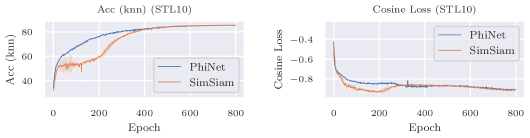
Table 11 and Table 12 present the CIFAR10 experiment results with varying batch sizes and weight decay. PhiNet shows equal or better performance than SimSiam across different batch size. The evaluation trends from KNN classification and linear probing are also consistent. It is also a consistent result that training on CIFAR10 performs poorly when cosine loss is used as the cortex loss function. Table 13 shows the results for STL10, where PhiNet performs comparably to SimSiam. However, as illustrated in Figure 7, PhiNet demonstrates better convergence in the early learning stages. In the early stages of training, when SimSiam is not stable, the cosine loss is smaller than that of the PhiNet, while as the training continues, the cosine loss increases again, in agreement with the PhiNet. This suggests that something close to mode collapse occurs in the early stages of SimSiam training, while PhiNet may suppress this collapse.

F.4 Computational Costs

Table.14 shows the memory consumption when training on CIFAR10. There is little overhead for PhiNet and X-PhiNet over SimSiam, as the maximum memory consumption during training is not only related to weights, but also to gradients and activation state. In fact, the GPU consumption is highly dependent on batch size, indicating that the gradient and activation state, which are dependent on batch size, are dominant in this setting.

Table 14: Comparison of GPU memory costs. This is a comparison of memory consumption when training on CIFAR10. We report batch sizes with 128 and 1024.
BYOL SimSiam Barlow PhiNet RM- X-PhiNet X-PhiNet
Twins SimSiam (MSE) (Cos)
BS=128 4.3(GB) 3.26(GB) 2.79(GB) 3.25(GB) 4.06(GB) 3.44(GB) 3.44(GB)
BS=1024 22.28(GB) 17.10(GB) 12.23(GB) 17.18(GB) 21.96(GB) 17.11(GB) 17.11(GB)

F.5 Stable Rank of Additional Predictor Layer

Refer to caption
Figure 8: The smaller the weight decay, the larger the rank of the additional predictor. We trained PhiNet on CIFAR10 with SGD and evaluate the lank for layers in additional predictor blocks.

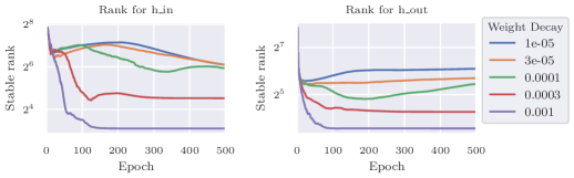
Figure.8 shows the rank for 2 linear layers in additional predictor blocks of PhiNet. We used stable rank in this figure and it is defined as $\operatorname{srank}(M)=\|M\|_{F}^{2}/\|M\|^{2}$, which is the lower rank of the standard rank and is more stabe to the small eigenvalues of $M$. According to this figure, the rank of the additional layer remains large when the weight decay is small, suggesting that the additional layer may play a more important role in learning when the weight decay is small.

Appendix G Experimental Settings

G.1 Settings for Training with CIFAR10, CIFAR100 and STL10

Table 15 shows the model and experimental setup for Figure 5, Table 9, Table 11, Table 12 and Table 13. Note that in the graph of sensitivity with respect to weight decay, we explored a widerer range of values. For linear probing evaluation, we trained the head layer by SGD for 100 epochs. For both CIFAR10 and STL10, we used 50,000 samples for training and 10,000 samples for testing. We have implemented it based on code that is already publicly available111https://github.com/PatrickHua/SimSiam.

Table 15: The experimental setups of Figure 5, Table 9, Table 11, Table 12 and Table 13.
Learning Optimiser SGD
Momentum 0.9
Learning Rate $0.03$
Epochs 800
Encoder Backbone ResNet18_cifar_variant1
Projector output dimension 2048
Predictor $h$ Latent dimension $m$ 2048
Hidden dimension $h$ and $g$ 512
Activation function ReLU
Batch normalization Yes
Predictor $g$ Latent dimension $m$ 2048
Hidden dimension $h$ and $g$ 512
Activation function ReLU
Batch normalization Yes
Computational resource GPUs V100 or A100

G.2 Settings for Training on ImageNet

In our ImageNet [41] experiments, we follow the formal implementation of SimSiam by Pytorch222https://github.com/facebookresearch/simsiam [11]. Table 16 shows the model and experimental setup for Table 1. For ImageNet, we used 1,281,167 samples for training and 100,000 samples for testing. We trained on the three seeds and obtained the mean and variance.

Table 16: The experimental setups of Table 1.
Learning Optimiser SGD
Momentum 0.9
Learning Rate $0.05$
Epochs 100
Encoder Backbone ResNet50
Projector output dimension 2048
Predictor $h$ Latent dimension $m$ 2048
Hidden dimension $h$ and $g$ 512
Activation function ReLU
Batch normalization Yes
Predictor $g$ Latent dimension $m$ 2048
Hidden dimension $h$ and $g$ 512
Activation function ReLU
Batch normalization Yes
Computational resource GPUs 4$\times$V100

G.3 Settings for Training on CIFAR-5m

CIFAR-5m [33] is a dataset that is sometimes used as a vision dataset for online learning [48, 42]. We experimented with CIFAR-5m in a setting similar to online learning. Note that CIFAR-5m has 5m samples, but we chose to train CIFAR-5m for 8 epochs, as most of the SimSiam training on CIFAR10 involves training for 800 epochs. We experimented with three learning rates: {0.03, 0.01, 0.003}, and selected the one that yielded the best results. For Barlow Twins, the learning rate of 0.03 does not converge, so 0.003 is chosen instead. For all other methods, a learning rate of 0.03 is selected. The model architecture is the same as in CIFAR 10.

G.4 Settings for Training on split CIFAR10, split CIFAR100 and split-CIFAR-5m

As a benchmark for evaluating continual learning, we used split CIFAR10 and split CIFAR100 [22]. Additionaly, we created split cifar-5m, which is inspired by split-CIFAR10 but uses CIFAR-5m dataset. In split CIFAR10 and split CIFAR5m, we split CIFAR10 and CIFAR-5m into 5 tasks, each of which contains 2 classes. In split CIFAR10 , we split CIFAR100 into 10 tasks, each of which contains 2 classes. The model architecture is the same as in CIFAR 10. The implementation of continual learning is based on the official implementation of Madaan et al. [29].

We evaluated the results using Average Accuracy and Average Forgetting. The average accuracy after the model has trained for $T$ tasks is defined as:

$$A_{T}=\frac{1}{T}\sum_{i=1}^{T}a_{T,i},$$ (8)

where $a_{t,i}$ is the validation accuracy on task $i$ after the model finished task $t$. The average forgetting is defined as the difference between the maximum accuracy and the final accuracy of each task. Therefore, average forgetting after the model has trained for $T$ tasks can be defined as:

$$F=\frac{1}{T-1}\sum_{i=1}^{T-1}\max_{t\in\{1,\ldots,T-1\}}\left(a_{t,i}-a_{T,i}\right)$$ (9)