Lattice Boltzmann methods for soft flowing matter

Abstract

Over the last decade, the Lattice Boltzmann method has found major scope for the simulation of a large spectrum of problems in soft matter, from multiphase and multi-component microfluidic flows, to foams, emulsions, colloidal flows, to name but a few. Crucial to many such applications is the role of supramolecular interactions which occur whenever mesoscale structures, such as bubbles or droplets, come in close contact, say of the order of tens of nanometers. Regardless of their specific physico-chemical origin, such near-contact interactions are vital to preserve the coherence of the mesoscale structures against coalescence phenomena promoted by capillarity and surface tension, hence the need of including them in Lattice Boltzmann schemes. Strictly speaking, this entails a complex multiscale problem, covering about six spatial decades, from centimeters down to tens of nanometers, and almost twice as many in time. Such a multiscale problem can hardly be taken by a single computational method, hence the need for coarse-grained models for the near-contact interactions. In this review, we shall discuss such coarse-grained models and illustrate their application to a variety of soft flowing matter problems, such as soft flowing crystals, strongly confined dense emulsions, flowing hierarchical emulsions, soft granular flows, as well as the transmigration of active droplets across constrictions. Finally, we conclude with a few considerations on future developments in the direction of quantum-nanofluidics, machine learning, and quantum computing for soft flows applications.

Keywords: Lattice Boltzmann methods; soft flowing matter; near-contact forces; mesoscale simulations; microfluidic; emulsions; foams.

I Introduction

Soft matter lives at the intersection between the three fundamental states of matter: gas, liquid, and solid. Much of its fascination draws from the fact that such intersection is all but a linear superposition of the three fundamental states, and supports instead genuinely new mechanical and rheological behavior, with important consequences for many applications in science and engineering Piazza (2012); Doi (2013); Fernandez-Nieves and Puertas (2016); Kleman and Lavrentovich (2003). The demise of linear superposition can be traced to the nonlinear interactions associated with the configurational degrees of freedom: for instance, foams are typically disordered assemblies of a gas (vapor) phase into a liquid water matrix and even though both phases are Newtonian, i.e. they respond to external load in direct proportion to the load intensity, once combined together, they develop a nonlinear and often non-local response. Given its paramount role in modern science and engineering, the quantitative study of soft matter has witnessed a burgeoning growth in the last decades Nagel (2017); Chen et al. (2010); Hamley (2003). This interest is further accrued by considering situations in which soft materials flow through confined geometries, since this gives rise to entirely new regimes and driven non-equilibrium steady states. In this review, we shall be concerned mostly with soft flowing systems characterized by a dispersed phase (droplets or bubbles) into a continuum matrix, say oil droplets in a water continuum, under strong geometrical confinement. Such specific systems have witnessed major development in the last decades mostly on account of progresses in experimental microfluidics, whereby one can control the spatial configurations of the droplets by simple experimental handles, typically the the ratio of oil to water mass flow and the geometrical setup of the microfluidic channel. By properly tuning such parameters, one can seamlessly move from dilute systems (droplet gas) to denser disordered states (droplet liquids) and finally even denser ordered ones, i.e. droplet solids with various topologies Raven and Marmottant (2009); Marmottant and Raven (2009) (see Fig.1).

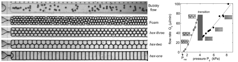
Figure 1: Droplet-based states of matter. Top left panel: a dilute ”gas” of droplets at low oil/water ratios. Second from top left: a ”liquid-like” collection of disordered droplets in near-contact. Third from top left: a ”solid-like” configuration of droplets with honeycomb topology. Fourth from top left: another ”solid-like” configuration of droplets with hexagonal symmetry (flowing crystal). Bottom: a one-dimensional flowing crystal. Right panel: Flow curve of a soft flowing foam. The figures are reproduced with permission from Ref.Marmottant and Raven (2009).

Even though one can pass from one phase to another by simply increasing the oil/water mass influx, the corresponding rheology does not respond linearly and sometimes not even smoothly. For instance, instabilities may arise whereby an increase in pressure no longer results in a corresponding increase in mass flow, but triggers instead a collapse of the mass flow, due to the inability of the droplets to undergo additional deformations to absorb the effects of an increasing pressure gradient. A new mechanism is needed to adjust the increasing pressure drive, a mechanism which materializes in the form of topological rearrangements of the droplet configurations such as to match interfacial dissipation at both external and internal boundaries with the pressure load.

Many different experiments can be performed with these droplet-based states of matter, by changing the geometrical and physical setup. For instance, Tang and collaborators studied the intriguing non-equilibrium pattern formation phenomena that occur in dense emulsions flowing in tapered channels Y. et al. (2016) (see Fig.2a,b). These authors report an unexpected order in the flow of a concentrated emulsion in a tapered microfluidic channel, in the form of orchestrated sequences of dislocation nucleation and migration events giving rise to a highly ordered deformation mode. This suggests that nanocrystals could be made to deform in a more controlled manner than previously expected, and also hints at possible novel flow control and mixing strategies in droplet microfluidics. On a similar although distinct vein, using a microfluidic velocimetry technique, Goyon et al. Goyon and Bocquet (2010) characterized the flow of thin layers of concentrated emulsions confined in gaps of different thicknesses by surfaces of different roughness. These experiments show clear evidence of finite size effects in the flow behavior, which can be interpreted in terms of a non-local viscosity of practical relevance for applications involving thin layers, e.g. chemical or geometrical coatings. Yet another important area of experimental microfluidics concerns the realization of hierarchical emulsions (droplets within droplets). For instance, double emulsions are highly structured fluids consisting of emulsion drops that contain smaller droplets inside. Although double emulsions are potentially of commercial value, traditional fabrication by means of two emulsification steps leads to very ill-controlled structuring. Using a microcapillary device, experimentalists managed to fabricate double emulsions that contained multiple internal droplets in a core-shell geometry. By manipulating the properties of the fluid that makes up the shell, it is possible to manufacture encapsulation structures with a high degree of control and reproducibility Utada et al. (2005); Datta et al. (2014) (see Fig.2,c,d,e). These microfluidic technologies have also opened intriguing avenues in microbiology, for the detection of pathogens, antibiotic testing, cell migration, and motility Kaminski et al. (2016); Bray (2000).

The latter, in particular, is crucial to a number of physiological and pathological processes, such as wound healing, embryonic development, and cancer metastasis. In many of such instances, cells are found to migrate through highly confined environments, such as dense tissues and interstices, dramatically impacting their morphology and mechanics. For instance, in Refs.Elacqua et al. (2018), the authors studied the dynamics of a cancer cell crossing a narrow constriction (whose design is inspired by physiologically-relevant conditions) and quantified shape deformations as the cell migrates through tiny pores (see Fig.2f,g). Similar dynamic behaviors have been shown in Refs.Davidson et al. (2015, 2014) using fibroblast cells moving in confined environments. In these respects, double emulsions may serve as a simplified model to study biological cells, where the innermost droplet would be a representation of a nucleus and the layer would mimic the cell cortex containing motor proteins, such as the actomyosin complex Choi et al. (2016); Mao et al. (2019).

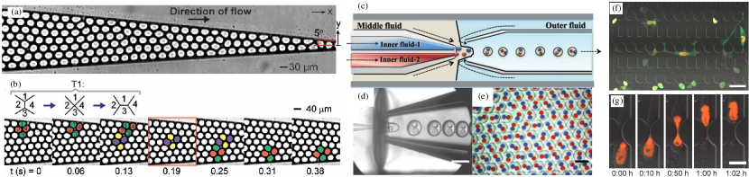
Figure 2: Left panel (a): A concentrated emulsion flowing in a tapered channel. (b): A cascade of T1 events (equivalent to a dislocation) involving converging and diverging droplets. From $t=0$ to $t=0.13$ red droplets diverge and green ones converge; from $t=0.13$ to $t=0.25$ purple droplets diverge and yellow ones converge; from $t=0.25$ to $t=0.38$ red droplets diverge and green one converge. The figures are reproduced with permission from Ref.Y. et al. (2016). (c) Sketch of a microfluidic device used for the production of multiple emulsions. (d)-(e) Experimental images of monodisperse double emulsions with two different inner drops. The figures are reproduced with permission from Ref.Adams et al. (2012). (f) Microfluidic chip modeling a sequence of constrictions typical of a porous tissue. (g) Close-up view of a cell nucleus crossing a narrow constriction. The figures are reproduced with permission from Ref.Elacqua et al. (2018).

The overall rheology of these complex states of soft flowing matter emerges from the competition/cooperation of multiple concurrent mechanisms acting across a broad spectrum of scales in space and time. Typically these encompass supramolecular interactions between near-contact surfaces at a scale of a few nanometers, all the way up to the overall size of the device, of the order of centimeters, spanning six decades in space and nearly twice as many in time in the process. Owing to the highly complex and nonlinear coupling between such mechanisms, analytical methods can only supply qualitative information, hence falling short of providing the degree of accuracy required by engineering design. At the same time, experimental methods have limited accessibility to the spectrum of the scales in action, such as the finest details of the flow configuration in the interstitial regions between interfaces or inside the droplets and bubbles.

Under such conditions, computer simulations emerge as an invaluable tool for gathering information that is otherwise inaccessible through theoretical approaches or experimental methods. Microfluidic flows are typically simulated using the principles of continuum fluid dynamics, as it is established that within the bulk flow, distant from sources of heterogeneities, the continuum assumptions remain valid down to nanometric scales. Bocquet and Charlaix (2010). In the vicinity of external surfaces, such as solid boundaries, or in the interstitial region between approaching interfaces, the continuum assumption may either go under question on sheer physical grounds, or simply become computationally unwieldy on account of the high surface/volume ratios characterizing microfluidic multiphase or multicomponent flows, such as the ones discussed in this review.

Until some two decades ago, the standard and only option out of the continuum was the resort to atomistic simulation, e.g. molecular dynamics (MD). Unfortunately, notwithstanding major sustained progress in the field, MD still falls short of reaching the scales of interest for microfluidics, both in space and more so in time. As a figure of reference, even a multibillion MD simulations can only cover three spatial decades, say from 1 nm to 1 micron, which is clearly far below the size of most experimental devices. Multiscale MD-Fluid procedures have been developed in the last decades but they are still laborious in day-to-day operations. In the last three decades a third, alternative avenue, based on the intermediate level described by kinetic theory, has generated a number of very appealing and useful mesoscale computational methods, either based on suitably discretized lattice versions of Boltzmann kinetic theory Succi (2018) or coarse-grained versions of stochastic particle dynamics, such as Dissipative Particle Dynamics Groot and Warren (1997) and Stochastic Rotation methods Gompper et al. (2009). Even though each of these methods comes with its strengths and weaknesses, we believe it is fair to state that the Lattice Boltzmann stands out as the one featuring an especially high degree of physical flexibility and computational efficiency across the full spectrum of scales of motion. This is why this review is focused on recent developments of the lattice Boltzmann (LB) method specifically aimed at capturing the complexity of soft flowing matter states, such as the ones described above.

The review is organized as follows. In Section II we provide a discussion of the basic physical scenario addressed here, namely soft flowing matter in microfluidic devices. In Section III we review the basic ideas behind the LB method for ideal and non-ideal fluids, including recent works accounting for near-contact interactions at nanometric scales, which are key for the description of dense systems under strong geometric confinement. In Section IV we provide an account of recent implementations of the above schemes on massively parallel computers, mostly aimed at minimizing the costs of memory access, an increasingly pressing topic for large-scale simulations. In Section V we discuss a list of selected applications, namely soft flowing crystals, soft granular media, dense emulsions with heat exchange, hierarchical emulsions under confinement, migration of active droplets through geometrical constrictions and flow through deep-sea sponges. The choice of such applications, which is inevitably partial and subjective, simply serves the purpose of conveying an idea of the broad spectrum of applications that can be handled by comparatively minor variants of the basic LB scheme. Finally, in Section VI we conclude with an outlook of potential future directions, namely the extension of current LB methodology to nanofluids with quantum interfacial effects, the use of machine learning to enhance LB simulations, and finally a few considerations on the prospects of quantum computing for soft flowing matter.

II Basic physics of microfluidic soft flowing matter

We shall refer to a two-component immiscible confined microfluidic flow composed of two fluids A and B, say water and oil for the sake of concreteness. An example of the system under study is shown in Fig.3, where a collection of monodisperse droplets (generated by the breaking of the jet of the dispersed phase (A) by the flow of the continuous one (B) in the orifice) flows in the exit channel of a flow focusser.

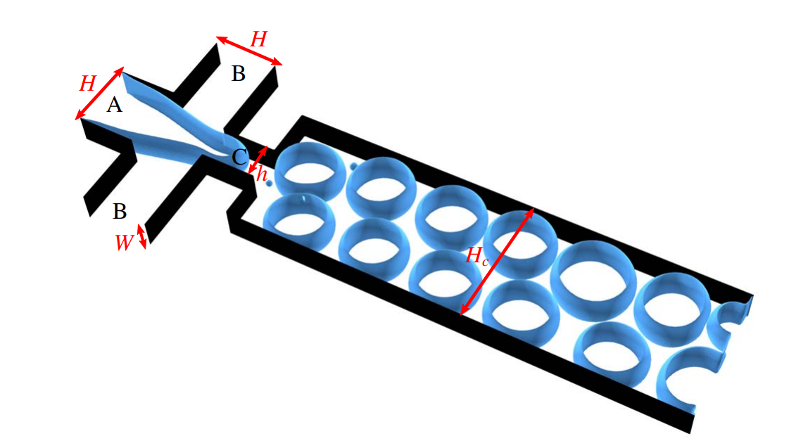
Figure 3: Typical structure of flow focuser and emulsion confined within. The device consists of three inlet channels (of height $H\simeq 200\mu$m and width $W\simeq 100\mu$m) supplying dispersed (A) and continuous phases (B), a narrower orifice (C) (of height $h\simeq 100\mu$m) and large outlet channel ($H_{c}\simeq 500\mu$m). The droplets emerging from the outlet of the microfluidic channel are evaporated away while the continuum phase is solidified by shining UV light into the fluid, so that one is left with a solid substrate with a regular sequence of holes (scaffold). The challenge is to preserve the stability of the soft flowing crystal at increasing speed, so as to maximize the production of scaffolding material. The figure is reproduced with permission from Ref.Montessori et al. (2019a).

The physics of this system is usually described by the standard equations of continuum mechanics, i.e. the Navier-Stokes equation

$$\rho D_{t}{\bf u}\equiv\rho\left(\partial_{t}{\bf u}+{\bf u}\nabla{\bf u}\right)={\bf F}_{pre}+{\bf F}_{dis}+{\bf F}_{cap}+{\bf F}_{nc}$$ (1)

supplemented with the incompressibility constraint

$$\nabla\cdot{\bf u}=0.$$ (2)

In the above ${\bf u}$ is the barycentric flow speed, $p$ the pressure and $\nu$ the kinematic viscosity. The total density $\rho$ is set to one for convenience, i.e. $\rho=\rho_{A}+\rho_{B}=1$.

The momentum equation contains four types of forces per unit volume. The first three, which represent the standard treatment, are the pressure gradient

$${\bf F}_{pre}=-\nabla p,$$

the dissipative force

$${\bf F}_{dis}=\rho\nu\nabla{\bf u},$$

and the capillary force

$${\bf F}_{cap}=\sigma\nabla\cdot\left[\bigg{(}\nabla^{2}\phi-(\nabla\phi)^{2}\bigg{)}{\bf I}-\frac{1}{2}\nabla\phi\nabla\phi\right],$$

where ${\bf I}$ is the unit matrix, $\sigma$ is the surface tension and

$$\phi=\frac{\rho_{A}-\rho_{B}}{\rho_{A}+\rho_{B}}$$ (3)

is a phase field (the order parameter) ranging between $-1$ and $+1$ telling the two fluids apart: namely $\phi=1$ in the A phase, $\phi=-1$ in the B phase, $\phi=0$ at the A/B interface.

The fourth term calls for some specific comments. It is intended to model ”near-contact” interactions, which arise whenever two interfaces come to a distance within the range of supramolecular forces, say around 10 nanometers. The physical origin of such near-contact forces may range from steric and depletion interactions to even Casimir-like interactions Derjaguin and Landau (1941); Verwey and Overbeek (1948); Lamoreaux (2004). However, in our case, we shall be agnostic regarding their physical basis and focus instead on the task of efficiently incorporating them into the LB solvers for soft flowing matter. Prior to turning to the numerics, a brief survey of basic physics is in order. It is often customary in microfluidics to define a reduced set of dimensionless groups accounting for the mesoscale physics of the system under scrutiny. The first one is the Reynolds number which measures the ratio between inertial and viscous forces and is defined as

$$Re=uH_{c}/\nu.$$ (4)

Since we are dealing with slow flows whose speeds are of the order of $u=1$ mm/s, inertial effects are usually small under strongly confined geometries, say 1 mm in the crossflow direction $H_{c}$, thus the Reynolds number is of the order of $Re\sim 1$. The next, possibly most important dimensionless group, is the capillary number

$$Ca=F_{vis}/F_{cap}=u\mu/\sigma,$$ (5)

where $\mu=\rho\nu$ is the dynamic viscosity. Typical values in microfluidic experiments are $Ca\sim 10^{-4}$, indicating that capillary forces are three-four orders above the dissipative ones, which are in turn comparable with inertial forces. Another way of rephrasing this is to say that the capillary speed $u_{cap}=\sigma/\mu$ is three-four orders of magnitude larger than the flow speed. Capillarity promotes shape changes towards sphericity and ultimately coalescence, which is definitely an unwanted effect for the design of droplet-based materials and applications in general. To this purpose, microfluidic experiments generally cater for a third dissolved species, namely surfactants, which prevent nearby interfaces from merging. The same role is played by repulsive near-contact interactions.

The competition between coalescence-promoting interactions (capillarity) and coalescence-frustrating ones (near-contact repulsion) lies at the heart of the complexity of these states of confined soft flowing matter. Such competition is measured by a nameless number that we dub $\mathcal{N}$ accordingly, defined as the ratio between near-contact and capillary forces. On dimensional grounds, we write the corresponding forces per unit volume as

$$F_{cap}\sim\sigma/D^{2}$$

and

$$F_{nc}=E_{nc}/h^{4},$$

where $E_{nc}$ is a typical energy scale of near-contact interactions and $h$ is the film thickness separating the two interfaces. As a result, we obtain:

$$\mathcal{N}=\frac{E_{nc}}{\sigma D^{2}}\frac{D^{4}}{h^{4}},$$ (6)

where $D$ is the diameter of the droplet. By taking $D\sim 100$ $\mu$m, $h\sim 10$ nanometers and $E_{nc}\sim kT$, we obtain $N\sim\frac{0.25\cdot 10^{-20}}{70\cdot 10^{-3}\cdot 10^{-16}}\times 10^{8}\sim 10^{3}$, indicating strong dominance of near-contact forces. However, a more realistic estimate is $E_{nc}/kT\sim 10^{-3}$, leading to $N\sim O(1)$ at $h=10$ nanometers. The above relation can also be written as

$$\mathcal{N}=\alpha\frac{k_{B}T}{\sigma D^{2}}\left(\frac{h}{D}\right)^{-4},$$ (7)

where we have defined $\alpha=E_{nc}/k_{B}T$. By choosing a reference value of $\sigma=0.1$ N/m and $D=100$ $\mu$m, we obtain

$$\mathcal{N}=4\times 10^{-12}\alpha\left(\frac{h}{D}\right)^{-4}.$$ (8)

Hence, the condition for the prevalence of near-contact interactions over capillary ones reads as

$$\frac{h}{D}<(4\alpha)^{1/4}10^{-3}.$$ (9)

Due to the weak dependence on $\alpha\simeq 10^{-3}$, the above formula shows that near-contact forces prevail below $h/D\sim 10^{-4}$. For the case in point, this occurs for $h$ below 10 nanometers (since $D\sim 100\mu m$). It is also of interest to observe that such near-contact interactions require dense regimes pretty close to the maximum packing fraction $\phi_{c}$ (see Fig.4). Based on the expression

$$\frac{h}{D}=\left(\frac{\phi_{c}}{\phi}\right)^{1/3}-1,$$ (10)

one concludes that $h/D\sim 10^{-4}$ implies $\phi/\phi_{c}\sim 1-10^{-4}/3$ which is indeed extremely close to the maximum packing fraction, a regime in which the material is basically a soft flowing solid.

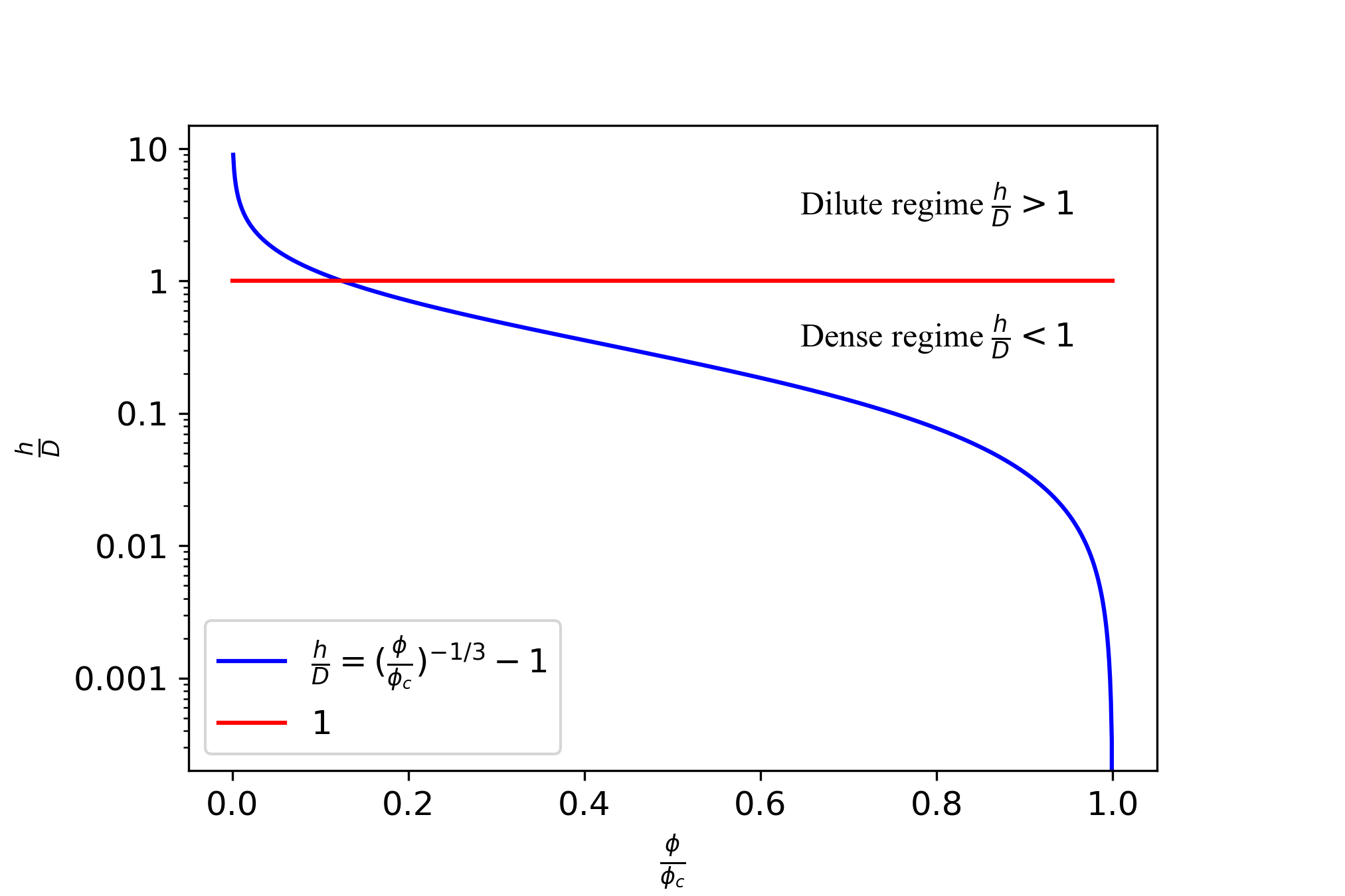
Figure 4: The $h/D$ parameter as a function of the relative volume fraction $\phi/\phi_{c}$. If $\phi/\phi_{c}\lesssim 0.2$, the mixture is in a dilute regime, thus near-contact forces can be neglected, whereas if $\phi/\phi_{c}>0.2$, these forces significantly affect the mechanical properties of the system.

It should be observed that while such values might be much smaller than the average, they can nonetheless occur as a result of strong dynamic fluctuations of the flowing multi-droplet configuration.

II.1 The multiscale scenario and Extended Universality

Since near-contact forces prevail at scales roughly below ten nanometers, predicting the rheological behavior at scales of experimental interest, say one centimeter, presents a complex nonlinear and nonlocal multiscale problem, spanning six decades in space and nearly twice as many in time. Whence the paramount role of advanced computational methods. Many methods are available in principle, but all of them face severe difficulties in handling the simulation of such a wide range of scales. LB methods are no exception in this respect. However, as anticipated earlier on, in this review we shall focus on LB mostly on account of its flexibility to incorporate non-equilibrium physics beyond hydrodynamics in realistically complex geometries, including coarse-grained interactions representing the effects of the unresolved scales on the resolved ones.

The usual computational strategy consists of splitting the six decades into a range of scales that are suitable to direct numerical simulation and a range of subgrid scales that need to be modeled. Current LB simulations can easily handle one billion lattice sites, thus covering three spatial decades, say from centimeters to tens of microns. Assuming molecular specificity to set in at about ten nanometer scale (which we dub supra-molecular scale), the remaining three decades can be covered either by grid-refinement or handled by coarse-grained models (see the sketchy Fig.5).

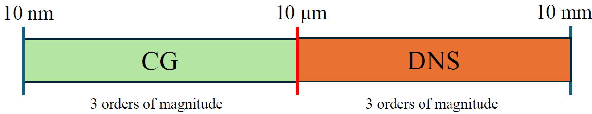
Figure 5: A schematic view of the typical scales accessible to coarse-grained (CG) and direct numerical simulations (DNS). The figure portrays a 3:3 balance between DNS and CG, which is the one adopted in most simulations discussed in this review. As computer power goes up, one can progressively extend the DNS bandwidth and shrink the CG one accordingly.

The former strategy requires about ten levels of grid refinement ($2^{10}=1024$) which involves a very substantial implementation effort, especially to secure a sustainable parallel efficiency. The latter is far simpler from the computational standpoint, but it is subject to issues of physical inaccuracy. Fortunately, at least for the (broad) spectrum of applications discussed in this work, it was found that the latter route provides a satisfactory description of the large-scale rheological behavior.

In hindsight, this is attributed to a sort of Extended Universality (EU) of the physics in point, meaning by this that the rheology of the soft matter systems under investigation is to a large extent insensitive to the details of the supra-molecular scales. More precisely, the essential effects of the near-contact interactions on large-scale rheology are largely dictated by their intensity relative to capillary forces, namely the dimensionless near-contact number $\mathcal{N}$ defined in the previous section. Values of $\mathcal{N}\sim 0.1$ are sufficient to prevent coalescence and secure a regular ”crystal-like” macroscale structure Montessori et al. (2019a). Upon increasing $\mathcal{N}$ disorder sets in and the ordered crystal tends to evolve into a disordered emulsion. Of course, one cannot expect EU to hold as a general rule, but for all the applications discussed in this work, it was found to provide a pretty satisfactory description of the complex rheology of the systems under investigation. In a broad sense, one could state that the LB simulations help unveiling the EU properties of soft flowing matter where they are.

III The lattice Boltzmann methods

In this section, we provide a short survey of the three major families of lattice Boltzmann methods, namely color-gradient (also termed chromodynamic), free energy, and pseudo-potential models. For an extensive discussion, we refer to specific textbooks, such as Refs. Succi (2018); Krüger et al. (2017); Sukop and Thorne (2006).

We begin by discussing some fundamental aspects of the theoretical background of non-ideal fluids, which are grounded in density functional theory (DFT). Subsequently, we will present the aforementioned numerical methods.

III.1 Density Functional and lattice kinetic theory

The kinetic theory of gases, as devised by Ludwig Boltzmann, was restricted to binary collisions of point-like particles hence formally limiting its application to dilute gases in the high Knudsen regimes. Huang (2008); Pathria and Beale (2011). Over the years, many efforts have been made to broaden the range of applicability of the kinetic theory to the characterization of dense gases and liquids, most of them facing significant challenges mainly connected with the emergence of infinities while handling higher-order, many body collisions. Although several strategies have been deployed to cope with such problems, the kinetic theory of dense, heterogeneous fluids remains a difficult subject to this day. A similar situation holds in the field of complex flows with interacting interfaces, often encountered in engineering, soft matter, and biology. In this context, a particularly interesting framework to deal with such complex flows is provided by the DFT Kohn (1999); Hohenberg and Kohn (1964); Kohn and Sham (1965).

The idea behind DFT is that much of the complexity connected with the physics of interacting, many-body fluid systems can be elucidated by tracking the dynamics of the fluid density, namely a single one-body scalar field. Of course, such a dynamics is subject to self-consistent closures, stemming from physically-compliant guesses of the generating functional from which the effective one-body equation for the density can be derived via minimization of the free-energy functional. DFT has been successfully applied to the description of quantum many-body systems, resulting in the formulation of fundamental theorems and associated computational techniques that form the basis of modern computational quantum chemistry Mourik et al. (2014). The same framework can be safely applied to classical systems encompassing interacting fluids with interfaces, and in the following, we proceed to illustrate such a picture in some more details.

The starting point of DFT is the definition of the free-energy functional

$$\mathcal{F}[\rho]=\int_{V}[f_{b}(\rho)+\frac{k}{2}(\nabla\rho)^{2}]dV,$$ (11)

where $f_{b}(\rho)$ is the bulk free energy depending on the local fluid density $\rho({\bf x})$, while the second term, multiplied by the constant $k$, represents the cost associated with the build up of interfaces within the fluid. The bulk component of the free energy determines the non-ideal equation of state via the Legendre transform $p=\rho df_{b}/d\rho-f_{b}$, while the interface term fixes the surface tension.

In the case of a binary mixture (two components A and B), it proves expedient to define an order parameter as in Eq.(3), which varies between $1$ in phase A and $-1$ in phase $B$ and takes value zero at the interface. Since the order parameter is conserved, the associated continuity equation reads

$$\partial_{t}\phi=-\nabla\cdot\left(M\nabla\frac{\delta\mathcal{F}[\phi]}{\delta\phi}\right),$$ (12)

where $M$ is the mobility, $\delta$ stands for the functional derivative and ${\cal F}[\phi]$ is a suitable free energy often expressed as a quartic polynomial in $\phi$ with square-gradient terms.

The order parameter is convected by the barycentric velocity of the two species, ${\bf u}({\bf x},t)$, which obeys the standard Navier-Stokes equations of fluids, augmented with an extra non-ideal pressure tensor, known as Korteweg tensor Landau and Lifshitz (1987), formally given by $K_{\alpha\beta}(\rho)=\frac{\delta^{2}\mathcal{F}}{\delta g_{\alpha}\delta g_{\beta}}$, where $g_{\alpha}\equiv\partial_{\alpha}\rho$ (Greek subscripts denote Cartesian components). The explicit form of the Korteweg tensor is as follows

$$K_{\alpha\beta}=\left(p+\frac{k}{2}(\partial_{\gamma}\phi)^{2}-k\phi\partial_{\gamma}\partial_{\gamma}\phi\right)\delta_{\alpha\beta}-k\partial_{\alpha}\phi\partial_{\beta}\phi,$$ (13)

where $p=p(\rho)$ is the ideal pressure. Finally, the divergence of the full pressure $\Pi_{\alpha\beta}$ tensor at the interface determines the mechanical force acting upon the fluid interfaces, $F_{\alpha}[\rho]=-\partial_{\beta}\Pi_{\alpha\beta}$ and the condition $F_{\alpha}=0$ selects the density profile realizing the mechanical equilibrium of the interface.

The coupling between the continuity and the Navier-Stokes equations with non-ideal pressure tensor provides a self-consistent mathematical framework describing the dynamics of the binary mixture. In such a framework, the lattice kinetic theory serves as a natural bridge between the microscopic physics and the macroscopic hydrodynamic interactions. Indeed, in the kinetic theory the main ingredient is represented by the non-ideal force term $S=F[\rho]\partial_{v}f$ (we omit subscripts and vector notation for simplicity), where $f$ is the probability density function. Such a forced-streaming term can be brought to the right-hand side of the kinetic equation and treated as a soft-collision term. The possibility to handle the partial derivative in velocity space by integrating it by parts permits to move the distribution function along characteristics $\Delta{\bf x}_{v}={\bf v}\Delta t$ and include the effect of soft forces as a perturbation to the free-streaming motion of $f$.

The above statement can be formalized as

$$f({\bf x}+{\bf v}\Delta t,{\bf v},t+\Delta t)-f({\bf x},{\bf v},t)=(C-S)dt,$$ (14)

where $C$ is the short-range collisional term which can be approximated by the Bhatnagar-Gross-Krook operator Bhatnagar et al. (1954)

$$C=(f^{eq}-f)/\tau.$$ (15)

Here, $f^{eq}$ is the local equilibrium distribution function and $\tau$ is a relaxation time.

The source collision term can also be turned into the following algebraic form

$$S=F[\rho]\sum_{l}s_{l}H_{l}(v),$$ (16)

where $s_{l}$ is the $l^{th}$ Hermite coefficient and $H_{l}$ the $l^{th}$ tensor Hermite basis. To note, the above relation can be obtained by performing an integration by parts in the velocity space of the continuous source term and by exploiting the recurrence relations of Hermite polynomials.

The advantage of this approach is that the streaming step (left-hand side of the equation) is exact (zero round-off error), being the distribution convected along linear characteristics, in stark contrast with the hydrodynamic formulation in which information moves along space-time dependent material lines defined by the fluid velocity. Thus, the above mathematical procedure allows the condensation of all the complex physics of moving interfaces into a purely local source term $S$. It is worth noting that, this ”perturbative” treatment works numerically as long as the magnitude of the source term is small enough to guarantee that the local Froude number is sufficiently small, i.e. $Fr=|\frac{a\Delta t}{v}|<<10^{-3}$ where $a=F/m$, a condition which may be broken in the presence of large density gradients.

Lattice density functional kinetic theories, as discussed above, are currently being used over an amazingly broad spectrum of soft-fluid problems, well beyond the original realm of rarefied gas dynamics. Indeed, in the last decades, kinetic theory has developed into a very elegant and effective framework to handle a broad spectrum of problems involving complex states of flowing matter Chapman and Cowling (1990); Pitaevskii and Lifshitz (1981); Riboff (2003). In particular, the LB method has emerged as an alternative and computationally efficient way to capture the physics of fluid dynamic phenomena, even in the presence of complex geometries and interacting fluid interfaces Succi (2018); Krüger et al. (2017). The next paragraph is dedicated to presenting the working principles of this method.

III.2 Basic ideas of the Lattice Boltzmann method

Let us now introduce the fundamental components that enable the functionality of the LB method. The LB equation states as follows:

$$f_{i}({\bf x}+{\bf c}_{i}\Delta t,t+\Delta t)-f_{i}({\bf x},t)=-\Omega_{ij}(f_{j}({\bf x},t)-f^{eq}_{j}),$$ (17)

where $f_{i}({\bf x},t)$ stands for the probability of finding a particle at lattice site ${\bf x}$ and time $t$ with a molecular velocity ${\bf u}={\bf c}_{i}$ along the i-th direction of the lattice support in use. In particular, the set of discrete velocities ${\bf c}_{i}$ with $i\in[0,b]$ is chosen to guarantee sufficient symmetry and to comply with the principles of conservation of mass-momentum. Typical examples of LB lattices are shown in Fig.6, where Fig.6a represents a two-dimensional mesh with nine discrete velocities (also termed as D2Q9 model) and Fig.6b represents a three-dimensional one with twenty-seven discrete velocities (D3Q27 model).

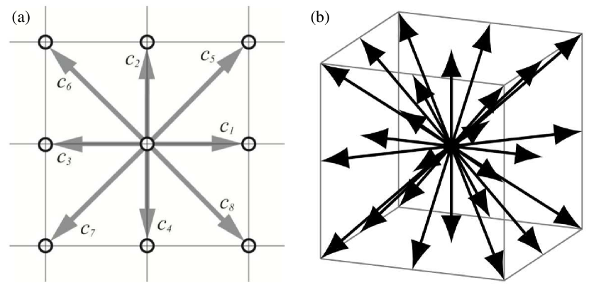
Figure 6: Two typical lattice meshes that are often used in LB simulations. (a) A two-dimensional lattice with nine discrete velocities ($i=0,...,8$). (b) A three-dimensional lattice with twenty-seven discreet velocities ($i=0,...,26$).

The term $\Omega_{ij}$ denotes a collision operator that can take the form of a single relaxation term $\Omega=1/\tau$ ($\tau$ being a relaxation time) Bhatnagar et al. (1954) or more complex structures, such as multiple-relaxation time operators Lallemand and Luo (2000); d’Humières (2002) and central-moment-based ones Fei et al. (2018a, b), to name notable examples.

The LB equation reported in Eq.(17) can be split into two parts: the left-hand side represents the free-flight of the distributions along lattice characteristics, also called the streaming step, while the right-hand side stands for a collisional relaxation step of the set of probability distribution functions towards a local thermodynamic, Maxwell-Boltzmann equilibrium $f^{eq}_{i}$. In particular, the local equilibrium is obtained by performing a Taylor expansion to the second order of the Mach number $Ma=u/c_{s}$

$$f^{eq}_{i}({\bf x},{\bf u})=w_{i}\rho\Big{[}1+\frac{{\bf c}_{i}\cdot{\bf u}}{c_{s}^{2}}+\frac{({\bf c}_{i}{\bf c}_{i}-c_{s}^{2}\mathbf{I}):{\bf u}{\bf u}}{2c_{s}^{4}}\Big{]},$$ (18)

where $c_{s}$ is the lattice sound speed, “:” denotes a tensor contraction between two second-order tensors, and $w_{i}$ represents a set of normalized weights. It is worth noting that the truncation is an outcome of lattice discreteness, allowing the recovery of Galilean invariance only up to a limited expansion in the Mach number.

The relevant hydrodynamic quantities can be obtained by computing the statistical moments of the distribution functions $f_{i}$ up to an order compliant with the moment isotropy of the lattice. At the Navier-Stokes level, the moment isotropy of the lattice must guarantee the retrieval of at least the first three moments of the distributions, namely density $\rho$, linear momentum $\rho{\bf u}$, and momentum flux tensor ${\bf\Pi}$

$$\rho=\sum_{i}f_{i}\left({\bf x},\,t\right),$$ (19)

$$\rho{\bf u}=\sum_{i}f_{i}\left({\bf x},\,t\right){\bf c}_{i},$$ (20)

$${\bf\Pi}=\sum_{i}f_{i}\left({\bf x},\,t\right){\bf c}_{i}{\bf c}_{i}.$$ (21)

The link between lattice Boltzmann equation and Navier-Stokes equation can be found through a Chapman-Enskog analysis Chapman and Cowling (1990), which essentially consists of a multiscale expansion of the distribution function about equilibrium (and of spatial and temporal derivatives) in the Knudsen number $\epsilon=\lambda/L$, where $\lambda$ is the molecular mean-free path and $L$ is a characteristic macroscopic length of the system. For small values of $\epsilon$ ($\epsilon\ll 1$), $\lambda$ is much smaller than $L$, hence a continuum theory would provide a reliable description of the fluid dynamics. It can be shown that this technique allows to recover both continuity and Navier-Stokes equation Krüger et al. (2017); Carenza et al. (2019), in which the kinematic viscosity is given by:

$$\nu=c^{2}_{s}\left(\tau-\frac{\Delta t}{2}\right).$$ (22)

The theory described so far is generally common to different LB methods simulating multiphase and multicomponent fluids at the microscale. However, the details of their implementation, as well as the way in which the physics of the fluid interface (i.e. pressure and surface tension) is computationally modeled, depends significantly on the type of LB adopted. In the next paragraph, we describe three widely used LB approaches to simulate soft flowing systems, namely color-gradient, free energy, and pseudopotential models.

III.3 Modern Lattice Boltzmann methods for soft matter

III.3.1 Color-gradient LB

In the color gradient LB for multicomponent flows, two sets of distribution functions are employed to track the evolution of two interacting fluid components. Following Eq.(17), the streaming-collision algorithm becomes

$$f_{i}^{k}\left({\bf x}+{\bf c}_{i}\Delta t,\,t+\Delta t\right)=f_{i}^{k}\left({\bf x},\,t\right)+\Omega_{i}^{k}(f_{i}^{k}\left({\bf x},\,t\right)),$$ (23)

where $k$ runs over the fluid components. The density $\rho_{k}$ of the $k^{th}$ component is given by the zeroth moment of the distribution functions

$$\rho_{k}\left({\bf x},\,t\right)=\sum_{i}f_{i}^{k}\left({\bf x},\,t\right),$$ (24)

while the total fluid density is

$$\rho=\sum_{k}\rho_{k}.$$ (25)

Also, the total momentum of the mixture is defined as the sum of the linear momentum of the two components

$$\rho{\bf u}=\sum_{k}\sum_{i}f_{i}^{k}\left({\bf x},\,t\right){\bf c}_{i}.$$ (26)

The collision operator $\Omega_{i}^{k}$ on the right hand side of Eq.(23) can be split into three components Gunstensen et al. (1991); Leclaire et al. (2012, 2017)

$$\Omega_{i}^{k}=\left(\Omega_{i}^{k}\right)^{(3)}\left[\left(\Omega_{i}^{k}\right)^{(1)}+\left(\Omega_{i}^{k}\right)^{(2)}\right],$$ (27)

where $\left(\Omega_{i}^{k}\right)^{(1)}$ is the standard BGK operator $\frac{1}{\tau}(f_{i}^{k,eq}-f_{i}^{k})$ Succi (2018), $\left(\Omega_{i}^{k}\right)^{(2)}$ performs the perturbation step Gunstensen et al. (1991), which builds up the surface tension and $\left(\Omega_{i}^{k}\right)^{(3)}$ is the recoloring step Gunstensen et al. (1991); Latva-Kokko and Rothman (2005), which promotes the separation between components, in order to minimize the mutual diffusion.

The correct form of the stress tensor can be obtained by imposing the constraints

$$\sum_{i}\left(\Omega_{i}^{k}\right)^{(2)} = 0$$ (28)

$$\sum_{k}\sum_{i}\left(\Omega_{i}^{k}\right)^{(2)}{\bf c}_{i} = 0,$$ (29)

which stems from the idea of continuum surface force Brackbill et al. (1992), where the surface tension is interpreted as a continuous transport coefficient across an interface, rather than as a boundary value condition on the interface.

By using a Chapman-Enskog expansion of the distribution functions, it can be shown that the hydrodynamic limit of Eq.(23) leads to the continuity and Navier-Stokes equations

$$\partial_{t}\rho+\nabla\cdot(\rho{\bf u}) = 0$$ (30)

$$\partial_{t}(\rho{\bf u})+\nabla\cdot(\rho{\bf u}{\bf u}) = -\nabla p+\nabla\cdot[\rho\nu(\nabla{\bf u}+\nabla{\bf u}^{T})]+\nabla\cdot\bm{\Sigma},$$

where $p=\sum_{k}p_{k}$ is the pressure and ${\bf\Sigma}$ is the non-ideal stress tensor. The latter can be written in terms of the perturbation operator and is given by

$$\bm{\Sigma}=-\tau\sum_{i}\sum_{k}\left(\Omega_{i}^{k}\right)^{(2)}{\bf c}_{i}{\bf c}_{i}.$$ (32)

An explicit expression of the surface tension $\sigma$, which is generated by $(\Omega_{i}^{k})^{(2)}$, can be obtained through the relation

$$\nabla\cdot\bm{\Sigma}={\bf F},$$ (33)

where ${\bf F}$ is a force inducing a stress jump across the interface. Following Refs.Brackbill et al. (1992); Liu et al. (2012), a general expression for the force is given by

$${\bf F}({\bf x},t)=\nabla\cdot[\sigma(\mathbf{I}-{\bf n}\otimes{\bf n})\delta_{I}],$$ (34)

where $\delta_{I}=\frac{1}{2}|\nabla\phi|$ is an index function which localizes the force on the interface, $\phi=\frac{\rho_{A}-\rho_{B}}{\rho_{A}+\rho_{B}}$ is the phase field associated to the components $A$ and $B$, and the normal ${\bf n}$ at the interface can be approximated by the gradient of the phase field, i.e. $\mathbf{n}=\nabla\phi/|\nabla\phi|$ Liu et al. (2012). Note that Eq.(34) is nothing but the stress jump across an interface given by ${\bf T}_{A}\cdot{\bf n}-{\bf T}_{B}\cdot{\bf n}=-\nabla\cdot[\sigma({\bf I}-{\bf n}\otimes{\bf n})]$, where ${\bf T}=-p{\bf I}+\rho\nu(\nabla{\bf u}+\nabla{\bf u}^{T})$ is the stress tensor.

By choosing

$$\left(\Omega_{i}^{k}\right)^{(2)}=\frac{A_{k}}{2}|\nabla\phi|\left[w_{i}\frac{(\vec{c}_{i}\cdot\nabla\phi)^{2}}{|\nabla\phi|^{2}}-B_{i}\right]$$ (35)

and substituting it into Eq.(28), Eq.(29) and Eq.(33), one gets the surface tension Leclaire et al. (2012)

$$\sigma=\frac{2}{9}(A_{A}+A_{B})\frac{1}{\bar{\omega}},$$ (36)

where $\bar{\omega}=2/(6\overline{\nu}-1)$ and $\overline{\nu}^{-1}=\frac{\rho_{A}}{\rho_{A}+\rho_{B}}\nu_{1}^{-1}+\frac{\rho_{B}}{\rho_{A}+\rho_{B}}\nu_{2}^{-1}$. In this model it is customary to assume $A_{A}=A_{B}$, thus $\sigma=\frac{4}{9}A\frac{1}{\bar{\omega}}$. In practical terms, the coefficients $A_{A}$ and $A_{B}$ are computed once the values of viscosity and surface tension are set. Finally, the coefficients $B_{i}$ in $(\Omega_{i}^{k})^{2}$ can be obtained by imposing the following isotropy constraints

$$\sum_{i}B_{i}=\frac{1}{3},\hskip 14.22636pt\sum_{i}B_{i}{\bf c}_{i}=0,\hskip 14.22636pt\sum_{i}B_{i}{\bf c}_{i}{\bf c}_{i}=\frac{1}{3}\mathbf{I}.$$ (37)

As previously mentioned, the perturbation operator $(\Omega_{i}^{k})^{2}$ allows for the building of the surface tension but does not guarantee the immiscibility of the fluid components. The latter condition is achieved by means of the recoloring step, which enables the interface to remain sharp and prevents the two fluids from mixing. Following Ref.Latva-Kokko and Rothman (2005), the recoloring operators are defined as follows

$$(\Omega_{i}^{1})^{(3)}(f_{i}^{A}) = \frac{\rho_{A}}{\rho}f_{i}^{*}+\beta\frac{\rho_{A}\rho_{B}}{\rho^{2}}\cos{\theta_{i}}f_{i}^{eq,0},$$ (38)

$$(\Omega_{i}^{2})^{(3)}(f_{i}^{B}) = \frac{\rho_{B}}{\rho}f_{i}^{*}-\beta\frac{\rho_{A}\rho_{B}}{\rho^{2}}\cos{\theta_{i}}f_{i}^{eq,0},$$ (39)

where $f_{i}^{*}=\sum_{k}f_{i}^{k,*}$ denotes the set of post-perturbation distributions, $\rho=\rho_{A}+\rho_{B}$, $\theta_{i}$ is the angle between the phase field gradient and the $i^{th}$ lattice vector, $f_{i}^{eq,0}=\sum_{k}f_{i}^{k}(\rho,{\bf u}=0)^{eq}$ is the total zero-velocity equilibrium distribution function Leclaire et al. (2012) and $\beta$ is a free parameter tuning the interface width, thus playing the role of an inverse diffusion length scale Latva-Kokko and Rothman (2005). In Montessori et al. (2018a), it has also been shown that the color gradient LB scheme can be further stabilized by filtering out the high-order non-hydrodynamic (ghost) modes emerging in the under-relaxed regime (i.e. $\tau\geq\Delta t$) Montessori et al. (2015); Zhang et al. (2006); Latt and Chopard (2006); Coreixas et al. (2017); Mattila et al. (2017); Hegele et al. (2018); Montessori et al. (2016). This improvement essentially allows the color gradient to operate at higher values of droplet speed minimizing the effects due to spurious currents and ghost modes Succi et al. (1995); Benzi et al. (1992); Montessori et al. (2018a, b).

Near-contact interactions.

In the color-gradient scheme, the effect of repulsive near-contact forces can be modeled, at the mesoscale, by including an additional term in the stress-jump condition Montessori et al. (2019a), which reads as follows:

$$\mathbf{T}_{A}\cdot{\bf n}-\mathbf{T}_{B}\cdot{\bf n}=-\nabla\cdot[\sigma(\mathbf{I}-{\bf n}\otimes{\bf n})]-\pi{\bf n}.$$ (40)

The last term $\pi[h({\bf x})]$ is responsible for the repulsion between neighboring fluid interfaces and $h({\bf x})$ is the distance, along the normal ${\bf n}$, between positions ${\bf x}$ and ${\bf y}={\bf x}+h{\bf n}$ of the two interfaces (see Fig.7).

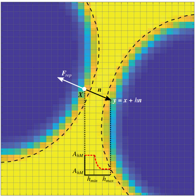
Figure 7: The figure shows a representation of the near-contact forces between two fluid interfaces (highlighted by a dotted curve). Once two droplets are in close contact, a repulsive force ${\bf F}_{rep}$ is switched on to prevent droplet merging. The blue region is the dispersed phase (droplets) while the yellow one is the continuous phase. The figure is reproduced with permission from Ref.Montessori et al. (2019a).

By neglecting surface tension variations along the interface (thus the stress tensor ${\bf T}$ can be approximated as $\mathbf{T}=-p\mathbf{I}$ (Brackbill et al. (1992)) and by projecting Eq.(40) along the normal at the interface, an extended Young-Laplace equation can be obtained (Chan et al. (2011); Williams and Davis (1992))

$$(p_{B}-p_{A})=\sigma(\nabla\cdot\vec{n})-\pi.$$ (41)

The additional repulsive term can be readily included within the LB framework through a forcing contribution acting only between fluid interfaces in near-contact

$${\bf F}_{rep}=\nabla\pi:=-A_{h}[h({\bf x})]{\bf n}\delta_{I},$$ (42)

where $A_{h}[h({\bf x})]$ is a parameter tuning the strength of the near-contact interactions (see Fig.7). A reasonable choice for $A_{h}$ suggests taking it constant for $h\leq h_{min}$ (where $h_{min}$ could correspond to two/three lattice sites separating opposite interfaces) and decreasing as $h^{-3}$ for $h>h_{min}$. Also note that, although the force in Eq.(42) depends solely on the distance between two fluid interfaces, its expression can be extended to account for local variations of distance caused by the spontaneous migration of the surfactant along the fluid interface Gupta et al. (2017).

We finally mention that, over the years, other methods have been proposed to model the physics of near-contact forces in these systems Nekovee et al. (2000); Love et al. (2001); Chen et al. (2000). However, unlike the approach discussed here where their effect is taken into account by introducing a repulsive force (as a mesoscale representation of supramolecular interactions), in these alternative methods two additional BGK-like equations are used, one for the distribution functions of a surfactant (which essentially prevents droplet coalescence) and another one for the relaxation of the average dipole vector. The latter is because the interaction among surfactant molecules depends on their relative distance and on their dipolar orientation. An important difference between these two approaches is that the color-gradient method augmented with near-contact forces only requires two sets of distribution functions regardless of the number of droplets, thus allowing for the simulations of mixtures with high volume fractions of droplets (see Section V) at a dramatically reduced computational cost.

III.3.2 Free-energy model

The free-energy approach is based on the idea that macroscopic physical quantities (such as chemical potential and pressure tensor) are derived from a free energy functional capturing the equilibrium properties of the system under study Swift et al. (1996, 1995); Krüger et al. (2017); Succi (2018). Unlike other models (such as the Shan-Chen approach Shan and Chen (1993); Shan and Doolen (1995), see next paragraph), this prescription allows to preserve the thermodynamic consistency of the model, since the fluid attains its thermodynamic equilibrium under the guidance of the free energy. Here we begin with a short description of the thermodynamics of the free energy LB of a multicomponent system, such as a water-oil mixture Swift et al. (1996, 1995), and then we discuss a few details about its numerical implementation.

In this model, a free energy functional can be generally written as an expansion of suitable order parameters, such as fluid density or relative concentrations describing the bulk properties, plus gradient terms capturing the physics of the interfaces. Hence, on a general basis, a free energy can be defined as follows

$${\cal F}=\int_{V}(f_{b}+f_{g})dV,$$ (43)

where $f_{b}$ is the bulk free energy leading to an equation of state in which different phases coexist, and $f_{g}$ is the interfacial term accounting for the energetic cost due to variations of order parameters.

The Landau theory allows us to derive these contributions analytically, namely

$$f_{b}=c_{s}^{2}ln\rho+\frac{a}{4}(\phi^{2}-1)^{2}$$ (44)

and

$$f_{g}=\frac{k}{2}(\nabla\phi)^{2},$$ (45)

where $\phi$ is a scalar phase field which distinguishes the bulk of the two interacting fluids. In $f_{b}$, the first term is the ideal gas free energy while the second one ensures the existence of two coexisting minima at $\phi=1$ and $\phi=-1$ for $a>0$, where the latter condition guarantees the immiscibility of the two fluid components. The interface free energy $f_{g}$ determines the surface tension, which can be calculated by integrating the free energy density across an interface. This leads to

$$\sigma=\int_{-\infty}^{\infty}\left[\frac{a}{4}(\phi^{2}-1)^{2}+\frac{k}{2}(\nabla\phi)^{2}\right]dx=\sqrt{\frac{8ak}{9}}.$$ (46)

A further thermodynamic quantity controlling the dynamic of the system is the chemical potential, which is defined as the functional derivative of the free energy with respect to the phase field. It is given by

$$\mu_{\phi}\equiv\frac{\delta{\cal F}}{\delta\phi}=-a\phi+a\phi^{3}-k\nabla^{2}\phi,$$ (47)

which is constant at equilibrium. In this condition, the equilibrium profile between the two coexisting bulk components is given by

$$\phi_{eq}=\mathrm{tanh}\left(\frac{2x}{\xi}\right),$$ (48)

where

$$\xi=\sqrt{\frac{2k}{a}}$$ (49)

is the interface width.

This physics is linked to the Navier-Stokes equations through a pressure tensor (i.e. the Korteweg tensor) $\Pi_{\alpha\beta}$, which can be derived upon imposing the condition $\partial_{\beta}\Pi_{\alpha\beta}=\phi\partial_{\alpha}\mu_{\phi}$. The latter leads to the following expression

$$\Pi_{\alpha\beta}=\left(p_{b}-\frac{k}{2}(\partial_{\gamma}\phi)^{2}-k\phi\partial_{\gamma}\partial_{\gamma}\phi\right)\delta_{\alpha\beta}+k(\partial_{\alpha}\phi)(\partial_{\beta}\phi),$$ (50)

where $p_{b}=c^{2}_{s}\rho+a\left(-\frac{1}{2}\phi^{2}+\frac{3}{4}\phi^{4}\right)$ is the equation of state. Once the thermodynamics is defined, the continuity and Navier-Stokes equations for a multicomponent fluid are equivalent to Eq.(30)-(LABEL:Nav_Stok_eq) with $\Pi_{\alpha\beta}=p\delta_{\alpha\beta}+\Sigma_{\alpha\beta}$.

Alongside the continuum equations, in the multicomponent free energy model one also needs an evolution equation for the phase field $\phi$. This is governed by the Cahn-Hilliard equation Cahn and Hilliard (1958)

$$\partial_{t}\phi+\nabla\cdot(\phi{\bf u})=\nabla\cdot(M\nabla\mu_{\phi}),$$ (51)

where the second term on the left-hand side represents an advection contribution due to the fluid velocity and the diffusive-like term (where $M$ is the mobility) on the right-hand side is the current driving the system towards equilibrium.

Multiphase field model.

In the same spirit of the color-gradient LB approach, the free-energy model can also be extended to simulate systems with more than two components and where coalescence is inhibited, such as dense emulsions Foglino et al. (2017). An emulsion of $N$ immiscible droplets, for example, can be described as a set of scalar fields $\phi_{n}$ ($n=1,....,N$) capturing the density of each droplet, whose dynamics obeys a corresponding set of advection-diffusion equation

$$\partial_{t}\phi_{n}+\nabla(\phi_{n}{\bf u})=\nabla(M\nabla\mu_{\phi_{n}}).$$ (52)

Once again, the chemical potential of each droplet is defined as $\mu_{\phi_{n}}=\delta{\cal F}/\delta\phi_{n}$, where ${\cal F}=\int_{V}fdV$. In this system, a suitable form of the free energy density $f$ is

$$f=\sum_{n=1}^{N}\left[\frac{a}{4}\phi_{n}^{2}(\phi_{n}-\phi_{0})^{2}+\frac{k}{2}(\nabla\phi_{n})^{2}\right]+\sum_{n,m,n<m}\epsilon\phi_{n}\phi_{m},$$ (53)

where the first term guarantees the existence of the minima $\phi_{n}=\phi_{0}$ (for example inside the $n$-th droplet) and $\phi_{n}=0$ (outside), and the second one accounts for the fluid interface. The positive constants $a$ and $k$ control surface tension and interface thickness, given by Eq.(46) and Eq.(49), respectively. Finally, the last term models a repulsive effect hindering droplet merging. This contribution slightly modifies the stress tensor, which includes an additional term proportional to $-\sum_{n}\phi_{n}\nabla\mu_{n}$.

Extension to active fluids.

In recent years, research on active matter in general and active fluids in particular has known a burgeoning growth Marchetti et al. (2013). Active matter presents a few distinctive features that set it apart from passive one, such as lack of reciprocity of pair interactions and the resulting breaking of time-reversal symmetry which triggers spontaneous motion. More often than not, however, the actual physical mechanisms responsible for the above features can be described in terms of additional internal degrees of freedom, coupled to the external ones (position and momentum) describing passive matter. As a result, from an operational standpoint, active systems can be regarded as passive systems with internal degrees of freedom coupled to the external ones in such a way as to sustain feedback loops with the environment. Therefore, the lattice Boltzmann method can be readily extended to handle active flowing matter as well. Indeed, over the last two decades, the free-energy lattice Boltzmann method has been successfully adapted to the simulation the hydrodynamics of active fluids and self-propelled droplets, in which the active fluid is segregated Carenza et al. (2019); Cates et al. (2009). As compared to an isotropic passive fluid, active fluids are made of individually oriented units supporting spontaneous symmetry breaking of rotational order, i.e. capable of developing orientationally ordered structures on macroscopic scales. This feature is generally captured by introducing an order parameter, such as the polar vector ${\bf p}({\bf x},t)$ or the tensor ${\bf Q}({\bf x},t)$, describing the ordering properties of the symmetry-broken phase, such as liquid crystals de Gennes and Prost (1993).

The thermodynamics of these systems is governed by a quantity akin to the free energy of Eq.(53) with further contributions depending on the additional fields, ${\bf p}({\bf x},t)$ or ${\bf Q}({\bf x},t)$. For instance, in the case of a polar active fluid droplet, the additional terms take the following form

$$f_{LC}(\phi,{\bf p})=-\frac{\alpha}{2}\frac{\phi-\phi_{cr}}{\phi_{cr}}|{\bf p}|^{2}+\frac{\alpha}{4}|{\bf p}|^{4}+\frac{\kappa}{2}(\nabla{\bf p})^{2},$$ (54)

where $\alpha$ and $\kappa$ are positive constants and $\phi_{cr}$ is the critical concentration for the transition from the unbroken isotropic phase $(|{\bf p}|=0)$ to the broken polar one $(|{\bf p}|>0)$. In the above, the first two terms represent the bulk free energy of the polar phase, while the last one describes the elastic penalty of the liquid crystal distortions in the single elastic constant approximation de Gennes and Prost (1993).

The polar field evolves according to an advection-relaxation equation of the form

$$D_{t}{\bf p}=-\frac{1}{\Gamma}\frac{\delta{\cal F}}{\delta{\bf p}},$$ (55)

where, besides the usual Lagrangian derivative, $D_{t}$ includes additional terms accounting for rigid rotations and deformations of the fluid element Carenza et al. (2019) and $\Gamma$ is the rotational inertia of the liquid crystal.

Finally, the fluid velocity obeys the Navier-Stokes equations, augmented with an active stress tensor of the form

$$\Pi_{\alpha\beta}^{act}\propto-\zeta\phi p_{\alpha}p_{\beta},$$ (56)

where $\zeta$ gauges the active strength, negative for contractile particles and positive for extensile ones. These two classes distinguish particles where the fluid is pulled towards the center of mass (i.e. contractile) from the ones where the fluid is pushed away from it (i.e. extensile). The active stress tensor is responsible for the coupling between the polar droplet and the surrounding fluid, leading to flow patterns that sustain the active motion of the droplet Hatwalne et al. (2004); Pedley and Kessler (1992).

Basic implementation.

Historically, two main free-energy lattice Boltzmann schemes have been used to simulate binary fluids. In the first one, the Cahn-Hilliard equation is solved by introducing a set of distribution functions $g_{i}({\bf x},t)$ connected to the phase field and the Navier-Stokes equation via the usual distribution functions $f_{i}({\bf x},t)$ defining zeroth, first and second order momenta. In the second one, the approach is hybrid, meaning that the Cahn-Hilliard equation is integrated via finite difference algorithms, while the Navier-Stokes is through a standard LB method. Both approaches have been widely used to simulate a variety of soft matter systems under confinement, such as liquid-vapor mixtures Gonnella et al. (2007), binary and ternary fluids Lamura et al. (1999); Xu et al. (2003, 2006); Gonnella et al. (2010); Tiribocchi et al. (2011a, 2021a, 2020a, 2021b, 2021c), liquid crystals Cates et al. (2009); Stratford et al. (2014); Lesniewska et al. (2024); Denniston et al. (2004); Sulaiman et al. (2006); Marenduzzo et al. (2004, 2008); Tiribocchi et al. (2011b, 2010, 2014, 2013) and active matter Marenduzzo et al. (2007a); Cates et al. (2008); Shendruk et al. (2017); Marenduzzo et al. (2007b); De Magistris et al. (2014); Negro et al. (2019); Bonelli et al. (2016, 2019); Tiribocchi et al. (2023a, b). Since some applications discussed in Section V are simulated using the second algorithm, we shortly recap its main features, while a detailed description of the first one can be found, for example, in Refs.Krüger et al. (2017); Carenza et al. (2019).

In the hybrid approach, the phase field $\phi$ obeys Eq.(51) and it is numerically updated in the following two steps.

1. An explicit Euler algorithm is used to integrate the convective term

   $$\phi^{*}({\bf x})=\phi-\Delta t_{FD}(\phi\partial_{\alpha}u_{\alpha}+u_{\alpha}\partial_{\alpha}\phi),$$ (57)

   where $\Delta t_{FD}$ is the time step of the finite difference scheme and the velocity ${\bf u}$ stems from the lattice Boltzmann equation. Note that the terms on the right-hand side are computed at time $t$ and lattice position ${\bf x}$.

2. The diffusive part is then updated

   $$\phi({\bf x},t+\Delta t_{FD})=\phi^{*}+\Delta t_{FD}\left(\nabla^{2}M\frac{\delta{\cal F}}{\delta\phi}\right)_{\phi=\phi^{*}},$$ (58)

where finite difference operators are calculated using a stencil representation to ensure isotropy of the lattice Tiribocchi et al. (2009); Thampi et al. (2013). Although more complex schemes have been used (such as predictor-corrector ones Denniston et al. (2004); Henrich et al. (2010)), this one combines satisfactory numerical stability and easy computational implementation.

The resolution of continuity and Navier-Stokes equations follows the prescriptions outlined in subsection III.2 properly extended to a binary fluid, basically meaning that the pressure tensor of the form of Eq.(50) must be implemented in the model. This can be done, for example, by modifying the constraints on the second moment of the distribution functions according to the following relation

$$\sum_{i}f_{i}^{eq}({\bf x},t)c_{i\alpha}c_{i\beta}=-\Pi_{\alpha\beta}+\rho u_{\alpha}u_{\beta}.$$ (59)

Note that, due to the symmetry of the left-hand side, this approach can be applied to systems in which the stress tensor is symmetric, such as a binary fluid. In the presence of anti-symmetric contributions (like in liquid crystals), the algorithm can be modified by introducing, on the right-hand side of Eq.(17), a suitable forcing term $p_{i}$ fulfilling the following relations

$$\sum_{i}p_{i}=0,\hskip 14.22636pt\sum_{i}p_{i}c_{i\alpha}=\partial_{\beta}\Pi_{\alpha\beta}^{anti},\hskip 14.22636pt\sum_{i}p_{i}c_{i\alpha}c_{i\beta}=0,$$ (60)

where $\Pi_{\alpha\beta}^{anti}$ represents the anti-symmetric component of the stress tensor. Further details on this model can be found in Refs.Krüger et al. (2017); Carenza et al. (2019).

III.3.3 Lattice pseudo-potential approach

An alternative route to simulate the hydrodynamics of multi-component mixtures is represented by the lattice pseudo-potential model, initially proposed in Refs. Shan and Chen (1993); Shan and Doolen (1995). Unlike the free-energy method, this one follows a ”bottom-up” approach by postulating a microscopic interaction between fluid elements from which a non-ideal equation of state as well as macroscopic observables, such as the surface tension and disjoining pressure, emerge (or can be eventually incorporated).

In this model, the crucial difference with the free-energy LB is that the pressure tensor is built from a force describing precisely such microscopic interactions. Assuming that the force between pairs of molecules is additive, one can expect that the interaction between fluid elements at positions ${\bf x}$ and ${\bf y}$ depends on the product $\rho({\bf x})\rho({\bf y})$. A suitable choice is Shan and Chen (1993)

$${\bf F}({\bf x})=-\int({\bf y}-{\bf x})G({\bf x},{\bf y})\psi({\bf x})\psi({\bf y})d^{3}{\bf y},$$ (61)

where $\psi$ is a density functional, called pseudo-potential, and $G$ is a kernel function accounting for the spatial dependence of the force.

In their work Shan and Chen (1993), Shan and Chen introduced the pseudo-potential as follows

$$\psi(\rho)=\rho_{0}[1-e^{-\rho/\rho_{0}}],$$ (62)

where $\rho_{0}$ is a reference density usually set to unity. The above term is bounded between $0$ and $\rho_{0}$ for any value of $\rho$, allowing the magnitude of the interaction force to be finite, even in the presence of large densities. This secures the stability of the model by switching the interaction off progressively as density increases, thereby smoothing the build-up of density divergences.

The implementation on the lattice follows a procedure partially akin to both color-gradient and free-energy LB, where different population sets represent a fluid component which evolves via a separate LB equation. The integral of Eq.(61) can be discretized by considering the interaction force to be short-ranged, so that the fluid element at the lattice site ${\bf x}$ can interact only with other neighboring elements at ${\bf y}={\bf x}+{\bf c}_{i}\Delta t$. Moreover, $G({\bf x},{\bf y})$ should be isotropic, thus depending on $|{\bf x}-{\bf y}|$ only. A common choice is $G({\bf x},{\bf y})=w_{i}G$ for ${\bf y}={\bf x}+{\bf c}_{i}\Delta t$ and zero otherwise.

The simplest form of the discretized Shan-Chen force for a multicomponent fluid is represented by a sum of pseudopotential interactions with nearest lattice neighbours

$${\bf F}_{\sigma}({\bf x})=-\psi_{\sigma}({\bf x})\sum_{\tilde{\sigma}}G_{\sigma\tilde{\sigma}}\sum_{i}w_{i}\psi_{\tilde{\sigma}}({\bf x}+{\bf c}_{i}\Delta t){\bf c}_{i}\Delta t,$$ (63)

where the sum runs over the lattice links, $\sigma$ and $\tilde{\sigma}$ are the two interacting components and $G_{\sigma\tilde{\sigma}}$ is a parameter setting the strength of their interaction and controlling the surface tension in the model. Unlike the free energy LB, here the surface tension is an emergent effect and can be explicitly calculated using the Young-Laplace test Krüger et al. (2017).

Thermodynamic consistency.

One may finally wonder to what extent the Shan-Chen model is supported by a consistent thermodynamic description. In the following, we show that an expression of the pressure tensor akin to that of the free-energy model can be obtained by properly expanding the pseudo-potential.

Following the derivation of Ref.Krüger et al. (2017) we consider, for simplicity, a multiphase mixture, where the forcing term is given by

$${\bf F}({\bf x})=-\psi({\bf x})G\sum_{i}w_{i}\psi({\bf x}+{\bf c}_{i}\Delta t){\bf c}_{i}\Delta t.$$ (64)

A Taylor expansion of $\psi({\bf x}+{\bf c}_{i}\Delta t)$ gives

$$\psi({\bf x}+{\bf c}_{i}\Delta t)= \psi({\bf x})+c_{i\alpha}\Delta t\partial_{\alpha}\psi({\bf x})$$ (65)

$$+ \frac{1}{2}c_{i\alpha}c_{i\beta}\Delta t^{2}\partial_{\alpha}\partial_{\beta}\psi({\bf x})$$

$$+ \frac{1}{6}c_{i\alpha}c_{i\beta}c_{i\gamma}\Delta t^{3}\partial_{\alpha}\partial_{\beta}\partial_{\gamma}\psi({\bf x})+...$$

Substituting Eq.(65) into Eq.(64) leads to

$$F_{\alpha}({\bf x})= - G\psi({\bf x})\sum_{i}w_{i}c_{i\alpha}\Delta t\biggl{(}\psi({\bf x})+c_{i\alpha}\Delta t\partial_{\alpha}\psi({\bf x})$$ (66)

$$+ \frac{1}{2}c_{i\alpha}c_{i\beta}\Delta t^{2}\partial_{\alpha}\partial_{\beta}\psi({\bf x})+....\biggr{)}.$$

Due to the symmetry of the lattice set, odd terms (i.e. $\sum_{i}w_{i}c_{i\alpha}$ and $\sum_{i}w_{i}c_{i\alpha}c_{i\beta}c_{i\gamma}$) vanish, thus leading to

$$F_{\alpha}({\bf x})=-G\psi({\bf x})\left(c_{s}^{2}\Delta t^{2}\nabla\psi({\bf x})+\frac{c_{s}^{4}\Delta t^{4}}{2}\nabla\nabla^{2}\psi({\bf x})\right).$$ (67)

The first term on the right-hand side is a gradient (of the form $-\frac{Gc_{s}^{2}\Delta t^{2}}{2}\nabla\psi^{2}({\bf x})$) that can be readily included in the equation of state of a multiphase fluid

$$p(\rho)=\rho c_{s}^{2}+\frac{c_{s}^{2}\Delta t^{2}G}{2}\psi^{2}(\rho),$$ (68)

while the second one resembles the surface tension contribution $k\rho\nabla\nabla^{2}\rho$ usually employed in diffuse interface models. Since, by definition,

$$\partial_{\beta}P_{\alpha\beta}=\partial_{\beta}(c^{2}_{s}\rho)-F_{\alpha},$$

it is finally possible to show that the Shan-Chen pressure tensor takes the following form

$$P_{\alpha\beta}= \left(\rho c_{s}^{2}+\frac{c_{s}^{2}G}{2}\psi^{2}+\frac{c_{s}^{4}G}{4}(\nabla\psi)^{2}+\frac{c_{s}^{4}G}{4}\psi\nabla^{2}\psi\right)\delta_{\alpha\beta}$$ (69)

$$- \frac{c_{s}^{4}G}{2}(\partial_{\alpha}\psi)(\partial_{\beta}\psi),$$

which differs from the thermodynamically consistent expression of the pressure tensor. However, in many practical situations where the density ratio between phases remains small, the surface tension and the density profiles obtained from Eq.(69) are acceptable and numerical stability is preserved. On the contrary, if the density ratio increases (typically higher than $10$), the stability can be improved by considering a Van der Waals-like equation of state (EOS), which dictates the pseudopotential according to

$$\psi(\rho)=\sqrt{\frac{2}{c_{s}^{2}\Delta t^{2}|G|}(p_{EOS}(\rho)-c_{s}^{2}\rho)},$$ (70)

where $p_{EOS}(\rho)$ is the desired equation of state. Such an approach, combined with a recent version of the entropic LB Hosseini et al. (2023) and a higher-order isotropic discretization of the gradient of the pseudo-potential, has permitted to simulate multiphase flows at Weber and Reynolds numbers above $10^{2}$ and $10^{3}$ respectively Montessori et al. (2017), unattainable by standard pseudo-potential methods.

III.4 Boundary conditions

We conclude this section with a short discussion on the boundary conditions used in the application (see Section V). Since the systems under study are either unbounded or are confined within a microchannel geometry, we focus on periodic boundaries and on solid ones modeling parallel flat walls, while we refer to specific textbooks Succi (2018); Krüger et al. (2017) for a general overview. It is worth noting that, despite the complexity of the systems under study, often involving confined deformable interfaces in close contact, the implementation of the boundary conditions (at least for the two aforementioned cases) follows well-known standard procedures. This is actually a key strength of the method, which proves capable of capturing the mesoscale physics of different examples of confined soft matter with minimal modifications to the existing algorithms.

Periodic boundary conditions.

We consider a two-dimensional one-component fluid (hence a single set of distribution functions), where periodic boundary conditions apply along the $x$ direction (see Fig.8) of a rectangular simulation box of size $L_{x}\times L_{y}$. We refer to the $D2Q9$ mesh numbered from $0$ to $8$, as shown in Fig.6. These conditions are typically used to isolate the bulk physics from actual boundaries (such as a wall) and essentially mean that the fluid leaving the lattice nodes located at $x=x_{N}$ re-enters at the ones located at $x=x_{1}$ and vice versa.

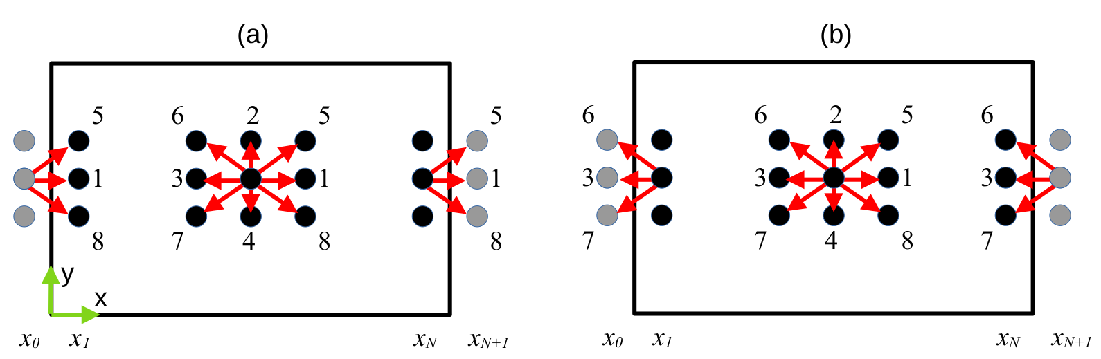
Figure 8: Periodicity along the $x$ direction. Black spots denote real nodes while grey ones indicate the buffer. Red arrows represent lattice velocity vectors, numbered according to Fig.6. (a) The distribution functions leaving from the leftmost column at $x_{N}$ fill in the virtual nodes on their rights, giving the populations on the opposite side at $x_{1}$. (b) A similar prescription holds for distribution functions leaving $x_{1}$ and giving the populations at $x_{N}$. The figure is inspired by Refs.Succi (2018); Krüger et al. (2017).

In terms of distribution functions, this prescription reads

$$f_{5}(x_{0},t)=f_{5}(x_{N},t)\hskip 28.45274ptf_{6}(x_{N+1},t)=f_{6}(x_{1},t)$$

$$f_{1}(x_{0},t)=f_{1}(x_{N},t)\hskip 28.45274ptf_{3}(x_{N+1},t)=f_{3}(x_{1},t)$$

$$f_{8}(x_{0},t)=f_{8}(x_{N},t)\hskip 28.45274ptf_{7}(x_{N+1},t)=f_{7}(x_{1},t)$$

for the inwards populations (left equations and Fig.8a) and for the outwards ones (right equations and Fig.8b). Note that, alongside the lattice nodes (black dots) of the simulation box, an additional layer of virtual nodes (grey dots) is included. During the boundary procedure, the distribution functions are copied in this buffer following the above equations and then they are updated for the streaming step.

No-slip boundary conditions.

A further typical boundary condition, often realized in a microchannel, is the one in which the fluid velocity at a solid surface is zero, thus there is no net motion of the fluid relative to the wall. This no-slip effect can be modeled by imposing that the distribution functions hitting a boundary node just reverse to where they start. The complete reflection ensures that normal and tangential components of the velocity at the wall vanish, thus the wall is actually impenetrable and the fluid does not slip on it. In terms of numerical implementations, no-slip conditions can be generally realized assuming that either the physical boundary lies exactly on a grid line or the boundary lies in between two grid lines. For illustrative purposes, here we shortly describe the first approach following Refs.Zou and He (1997).

We consider a one-component fluid confined within a microchannel consisting of two flat parallel walls and focus, for example, on the top one (see Fig.9). Similar considerations hold for the opposite wall.

Once the propagation step is completed, distribution functions $f_{0}$, $f_{1}$, $f_{5}$, $f_{2}$, $f_{6}$ and $f_{3}$ (continuous red arrows) are known while $f_{7}$, $f_{4}$ and $f_{8}$ (dotted red arrows) are unknown. These ones can be determined by using Equations (19) and (20).

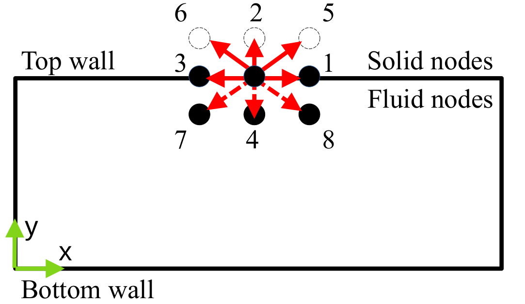
Figure 9: The figure is inspired by Ref.Succi (2018); Krüger et al. (2017).

Requiring that, at the wall, the fluid velocity is zero, the following equations hold

$$\rho = \sum_{i}f_{i}\rightarrow f_{7}(t)+f_{4}(t)+f_{8}(t)=$$

$$\rho-[f_{0}(t)+f_{1}(t)+f_{5}(t)+f_{2}(t)+f_{6}(t)+f_{3}(t)],$$

$$\rho u_{x,w} = \sum_{i}f_{i}c_{ix}=0\rightarrow f_{8}(t)-f_{7}(t)=$$

$$\hskip 69.70915ptf_{6}(t)-f_{5}(t)+f_{3}(t)-f_{1}(t),$$

$$\rho u_{y,w} = \sum_{i}f_{i}c_{iy}=0\rightarrow f_{7}(t)+f_{4}(t)+f_{8}(t)=$$

$$\hskip 69.70915ptf_{5}(t)+f_{2}(t)+f_{6}(t).$$

One can thus find the density in terms of known populations as

$$\rho=f_{0}(t)+f_{1}(t)+f_{3}(t)+2[f_{5}(t)+f_{2}(t)+f_{6}(t)]$$

and the unknown terms using the bounce-back rule for the distribution functions normal to the wall. The final set of equations reads

$$f_{4}(t) = f_{2}(t)$$

$$f_{7}(t) = f_{5}(t)+\frac{1}{2}[f_{1}(t)-f_{3}(t)]$$

$$f_{8}(t) = f_{6}(t)-\frac{1}{2}[f_{1}(t)-f_{3}(t)].$$

Further extensions of this approach aimed at guaranteeing improved numerical stability have also been proposed Lamura and Gonnella (2001); Tiribocchi et al. (2011a).

Boundary conditions of the phase field.

In confined systems studied by means of the hybrid free energy LB, it is also necessary to impose boundary conditions for the scalar field $\phi$. It is often customary to adopt either neutral wetting or no-wetting conditions, where the former are achieved by setting

$$\frac{\partial\mu}{\partial z}=0,\hskip 14.22636pt\frac{\partial\nabla^{2}\phi}{\partial z}=0$$ (71)

at the walls ($z$ being the vertical direction). The first one ensures density conservation while the second one guarantees the wetting to be neutral. These conditions are implemented by imposing that $\mu_{|z=\{0,L_{z}\}}=\mu_{|z=\{1,L_{z-1}\}}$ and $\nabla^{2}\phi_{|z=\{0,L_{z}\}}=\nabla^{2}\phi_{|z=\{1,L_{z-1}\}}$, where a stencil representation of finite difference operators is generally used. No wetting boundaries are enforced by substituting the second equation with the condition $\phi=\phi_{0}$ at the first and second lattice nodes along the horizontal direction, where $\phi_{0}$ is the value of one of the coexisting densities near the walls. In an emulsion, for example, $\phi_{0}$ would be the density of the dispersed phase.

IV Recent Lattice Boltzmann HPC implementations

In recent years, much work has been directed to developing advanced computational tools for the simulations of complex fluids on high performance computing (HPC) architectures. Indeed, the investigation of the flowing properties of confined soft materials often poses major multiscale challenges, due to the need to describe multi-component systems in centimeter-sized devices while retaining the physics of near-contact interactions. In this respect, standard LB approaches suffer a series of issues, the first being the relatively low arithmetic intensity, which varies between 1 and 5 Flops/Byte ratios depending on the specific implementation. Consequently, the LB method is often recognized as a memory-bound problem, as its efficiency is constrained by the memory access time on computing systems Succi et al. (2019). This problem is due to the necessity to directly store probabilistic distributions involving a set of approximately $b\sim 20-30$ discrete populations $f_{i}$ (where $i=0,...,b$ for each lattice point), clearly outnumbering the number of related hydrodynamic fields, which are a single scalar density $\rho$, the flow velocity $u_{\alpha}$ ($\alpha=1,3$), and momentum-flux tensor $\Pi_{\alpha\beta}$ (a $3\times 3$ symmetric tensor), amounting to 10 independent fields in total. Therefore, the LB method demands roughly double the memory compared to a corresponding computational fluid dynamics method based on Navier-Stokes equations. This redundancy buys several major computational advantages, primarily the fact that streaming is exact and diffusion is emergent (no need for second-order spatial derivatives to describe dissipative effects), which proved invaluable assets in achieving outstanding parallel efficiency across virtually any HPC platforms, also in the presence of real-world complex geometries Succi (2018). These extra-memory requirements put a premium on strategies aimed at minimizing the cost of data access in massively parallel LB codes.

Considering the extensive application of the LB method across various scales and regimes, it is crucial to devise strategies that mitigate the effect of data access on upcoming (exascale) LB simulations. Numerous such strategies have been previously established, which rely on hierarchical memory access Succi et al. (2019), data arrangement in the form of an array of structures and structure of arrays enhancing the data-contiguity Shet et al. (2013), and crystallographic lattice schemes that double the resolution for a specific level of memory usage Namburi et al. (2016).

A number of other approaches focus on reducing memory occupancy without significantly compromising the simulation quality. They can be categorized into three groups: the first one centers on the algorithmic implementation of the streaming step, the second one leverages diverse numerical representations to rounding in floating point arithmetic, and the third one avoids the direct storage of the probabilistic information by exploiting a reconstruction procedure of distributions from the hydrodynamics fields via Hermite projection.

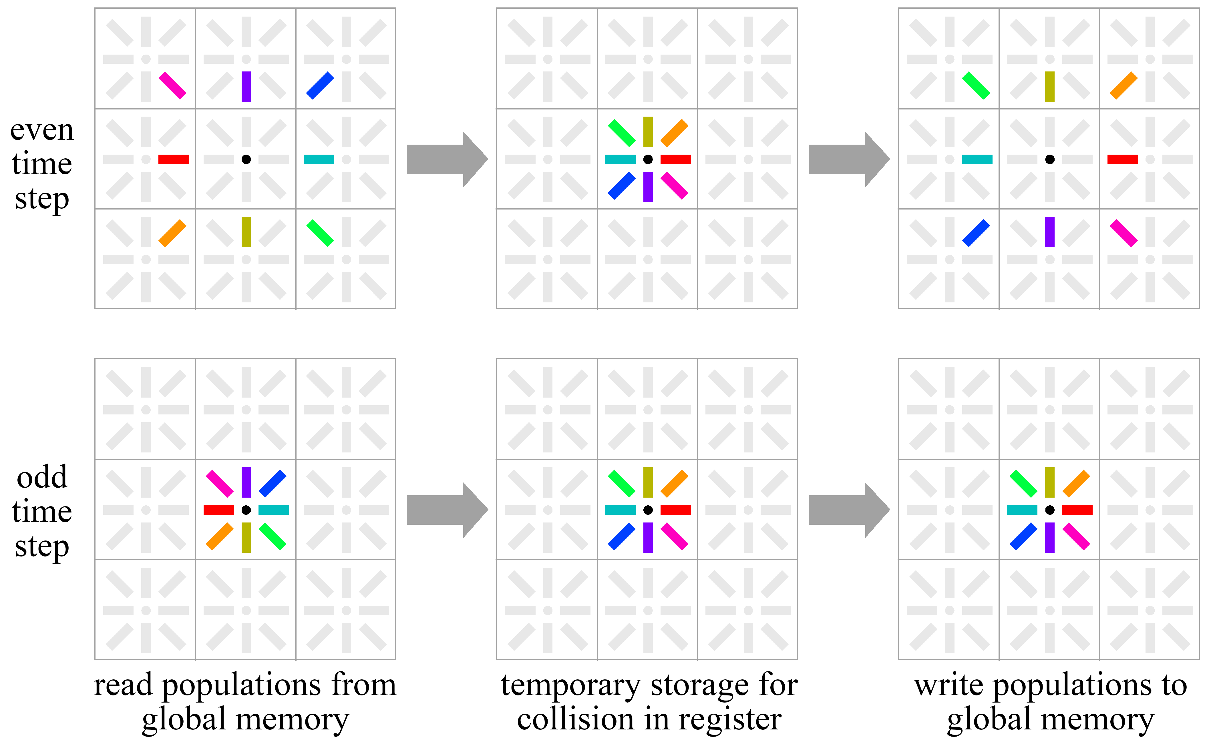
Figure 10: A sketch showing the AA-Pattern in-place streaming scheme by Bailey et al. Bailey et al. (2009). Note that the populations are always stored in the same memory location from where they were fetched. Hence, only a single copy of the population needs to be stored. The figure is reproduced with permission from Ref. Lehmann (2022).

First group.

Notable instances of the first strategy are the so-called “in-place” streaming, such as AA-Pattern and esoteric twist Lehmann (2022); Geier and Schönherr (2017). These approaches avoid using a double memory space to store the probabilistic populations; rather, they are aimed to read, compute, and write the results of the LB algorithm on the same memory space, thus halving the memory requirement. However, a race condition problem emerges when adjacent lattice points are handled simultaneously on parallel HPC clusters based on GPUs because the exact order of the floating-point operation execution is random Lehmann (2022). Consequently, more threads could read a value from a memory address already updated by another concurrent thread. To circumvent this issue, Bailey et al. Bailey et al. (2009) proposed an implementation strategy in which a streaming step, followed by a collision and another streaming step, are performed at even time steps while the collision step and a direction shift are executed at odd time steps only (see Fig.10). Thus, the algorithm, unlike the classical AB-pattern, reads the populations from copy A and writes back to the same copy A in place, whence the name the AA-pattern. Similarly, the esoteric twist in-place streaming scheme Geier and Schönherr (2017) and its variants (such as esoteric pull and esoteric push Lehmann (2022)), split the time integration into even and odd steps, performing the streaming of half of the set of populations (e.g. populations with negative directions only) in the even time step, while the set of the remaining directions is streamed in the odd time step. Hence, a precise set of shifting rules is applied at the end of the even and odd time steps to resemble the correct pattern every two time steps Lehmann (2022). However, the implementation of esoteric schemes is generally less straightforward since the populations are not always stored in the right positions, a drawback that further complicates a correct design of the boundary conditions. Nonetheless, both approaches, AA-Pattern and esoteric twist, halve the memory requirements alongside the number of data accesses to the global memory.

Second group.

The second strategy employs a single precision (instead of a double one) or a mixed single precision/half-precision representation which reduces the total memory usage by a factor of two without compromising the simulation quality Lehmann et al. (2022); Gray and Boek (2016). This approach was initially introduced by Skordos Skordos (1993), who showed that if the distribution functions are adjusted by negating the equilibrium zero-velocity distribution function, the probabilistic populations have the potential to maintain more significant bits during the execution of floating-point operations, thus increasing the computational precision. This idea was further developed in Ref.Gray and Boek (2016), where the dependence on the velocity of the accuracy of LB calculations, affecting the previous approach, was removed. More specifically, this method requires a modification of distribution functions and moments as follows. Using the symbols (float32) and (float64) to indicate the cast operators forcing a data type to be converted into single (32 bits/4 bytes) and double (64 bits/8 bytes) floating point precision, and writing

$$f_{i}({\bf x},t)=f_{i}^{eq}(\rho_{0},{\bf u}_{0})+\delta f_{i}({\bf x},t),$$ (72)

where $\rho_{0}$ and ${\bf u}_{0}$ are reference values (taken for simplicity equal to one and zero, respectively), the populations can be stored on the global memory saving only the extra term $[\delta f_{i}({\bf x},t)]_{\text{32bit}}=(\text{float32})(f_{i}({\bf x},t)-f_{i}^{eq}(\rho_{0},{\bf u}_{0}))$. Here the subscript $[\cdot]_{\text{32bit}}$ remarks that the values were saved in single floating-point precision (FP-32), while the precision in the floating-point operations is retained in double precision (FP-64). Thus, in a mixed-precision paradigm (FP-64/FP-32), the LB Eq.(17) with the BGK collision operator can be rewritten as

$$[\delta f_{i}({\bf x}+{\bf c}_{i}\Delta t,t+\Delta t)]_{\text{32bit}}=(\text{float32})\biggl{\{}\omega\delta f_{i}^{eq}+$$

$$(1-\omega)(\text{float64})[\delta f_{i}({\bf x},t)]_{\text{32bit}}\biggr{\}},$$ (73)

where $[\delta f_{i}({\bf x},t)]_{\text{32bit}}$ is first converted to double precision by the cast operator $(\text{float64})$. Hence, all the floating point operations were carried out in double precision with $\delta f_{i}^{eq}$ defined as

$$\delta f_{i}^{eq}=f_{i}^{eq}(\rho,{\bf u})-f_{i}^{eq}(\rho_{0},{\bf u}_{0})=w_{i}\Big{[}\frac{{\bf c}_{i}\cdot{\bf u}}{c_{s}^{2}}+\frac{({\bf c}_{i}{\bf c}_{i}-c_{s}^{2}\mathbf{I}):{\bf u}{\bf u}}{2c_{s}^{4}}\Big{]}+w_{i}(\rho-\rho_{0}),$$ (74)

with ${\bf u}_{0}=0$. Lastly, the result of Eq.(73) is again converted in single precision by applying the cast operator $(\text{float32})$ and stored in the global memory. The macroscopic hydrodynamics fields can be computed as

$$\rho=\sum_{i}(\text{float64})[\delta f_{i}({\bf x},t)]_{\text{32bit}}+\rho_{0},$$ (75)

$$\rho\vec{u}=\sum_{i}(\text{float64})[\delta f_{i}({\bf x},t)]_{\text{32bit}}{\bf c}_{i}.$$ (76)

Note that the distributions $\delta f_{i}(\vec{x},t)$ are centered around zero and shifted by $f_{i}^{eq}(\rho_{0},\vec{u}_{0})$, which means that the accuracy of the summation of small differences is not limited by the order of magnitude of the density $\rho_{0}$. Further, the summation can be performed with double precision accuracy. Recently, Lehmann et al. Lehmann et al. (2022) implemented the same strategy exploiting a mixed precision approach (FP-32/FP-16), where the floating-point operations are carried out in single precision, while the extra population terms are saved in half-precision (16 bits/2 bytes) $[\delta f_{i}(\vec{x},t)]_{\text{16bit}}$. In particular, they introduced a customized half-precision number format (FP16C) that halved truncation error compared to the standard IEEE-754 half-precision floating-point format FP16 in LBM applications Lehmann et al. (2022). However, benchmarks on the Karman vortex street in two dimensions have shown the presence of numerical noise in the third decimal digits, where the vorticity is compared between the mixed precision platforms FP64/32 and FP32/16C (see Fig.11). In concrete numbers, it is possible to quantify the LB performance in terms of a billion lattice sites per second (GLUPS), namely the number of updated lattice nodes per second reported in billions. For instance, Lehmann et al. Lehmann et al. (2022) measured the performance equal to 8.5 GLUPS on a single GPU NVIDIA A100 PCIe with 40GB RAM implementing the AA-Pattern in-place streaming scheme for a single component BGK LB model in a single precision floating point precision for storage and floating point operations and achieving a performance peak of 16 GLUPS by adopting the mixed precision approach (FP-32/FP-16).

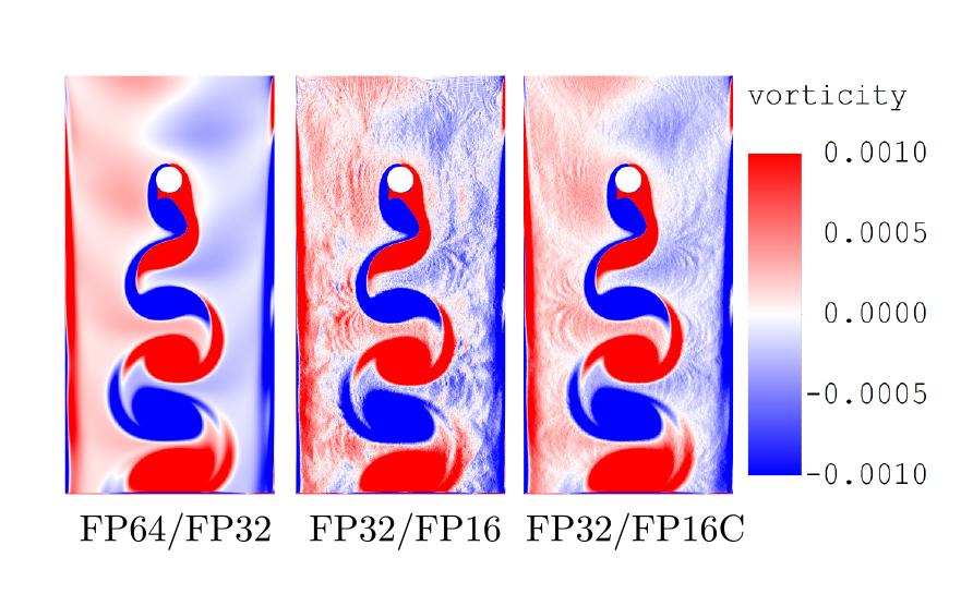
Figure 11: LB simulations of the Karman vortex street in two dimensions using the population shifting approach on various mixed floating-point precision platforms. The vorticity lies in the zoomed range of $\pm 0.001$, after $10^{5}$ LB time steps. For the 16-bit formats, noise is present in low vorticity regions. The figure is reproduced with permission from Ref. Lehmann et al. (2022).

Third group.

The third strategy for managing memory usage is grounded on the ideas of Ladd and Verberg Ladd and Verberg (2001), in which a memory reduction could be achieved by solely storing hydrodynamic fields and their gradients. This concept hinges on the fact that the probabilistic data needed to execute any LB method can be dynamically reconstructed using the available hydrodynamic quantities, thus eliminating the need for population storage. This is especially beneficial for multi-component and multi-species applications transported by a common flow field in which a single hydrodynamic field (i.e. the density) is needed rather than a full kinetic representation with $O(30)$ populations. A similar logic applies to flows that are far from equilibrium or involve relativistic hydrodynamics, which require higher-order lattices, sometimes involving hundreds of discrete populations per species. All methods based on this third approach typically rely on a moment-based representation of the LB, bypassing the direct storage of the probabilistic populations along each direction of the lattice. Among these, noteworthy implementations include the recently introduced lightweight LB (LLB) and thread-safe LB (TSLB) methods Tiribocchi et al. (2023c); Montessori et al. (2023, 2024), which are based on the reconstruction of probabilistic distributions via Hermite projection.

As in standard LB methods, the moment-based approach can be built starting from a set of distribution functions $f_{i}$ where each $f_{i}$ can be expanded around the equilibrium value

$$f_{i}=f_{i}^{(0)}+f_{i}^{(1)}+f_{i}^{(2)}+f_{i}^{(3)}+\dots,$$ (77)

being $f_{i}^{(0)}\stackrel{{\scriptstyle\triangle}}{{=}}f_{i}^{eq}(\rho,{\bf u})$ Krüger et al. (2009); Latt and Chopard (2006); Zhang et al. (2006); Ladd and Verberg (2001). All other components $f_{i}^{(k)}$ are sought in the order $O(\epsilon^{k})$, where $\epsilon$ is the Knudsen number with $\epsilon\ll 1$. Using a multiscale Chapman-Enskog expansion Chapman and Cowling (1990), it can be shown that only the first two terms, $f_{i}^{(0)}$ and $f_{i}^{(1)}$, are sufficient to recover (asymptotically) the Navier-Stokes equation Krüger et al. (2017); Latt et al. (2008). Consequently, one can write $f_{i}=f_{i}^{(0)}+f_{i}^{(1)}+O(\epsilon^{2})$ and identify $f_{i}^{(1)}=f_{i}-f_{i}^{(0)}+O(\epsilon^{2})$ as the non-equilibrium hydrodynamic term, apart from $O(\epsilon^{2})$ contributions. Therefore, if a relation between the term $f_{i}^{(1)}$ and the hydrodynamic fields is known, the distribution functions can be reconstructed without the direct storage of the probabilistic populations.

Such relation can be efficiently obtained by resorting to the regularization procedure Latt and Chopard (2006), whose main goal is to convert $f^{neq}_{i}=f_{i}-f_{i}^{(0)}$ into a set of non-equilibrium distributions lying on a Hermite subspace spanned by the first three statistical moments $\rho$, $\rho\mathbf{u}$ and $\Pi^{neq}$ Zhang et al. (2006). More specifically, by introducing Hermite polynomials and Gauss-Hermite quadratures, $f_{i}^{neq}$ is given by Shan et al. (2006); Montessori et al. (2015)

$$f^{neq}_{i}=w_{i}\sum_{n}\frac{1}{n!}\mathbf{a}^{n}\mathcal{H}^{n}(\mathbf{c}_{i}),$$ (78)

where $\mathcal{H}^{n}(\mathbf{c}_{i})$ and $\mathbf{a}^{n}=\sum_{i}\hat{f}^{neq}_{i}\mathcal{H}^{n}(\mathbf{c}_{i})$ are n-th order rank tensors. The former is the standard n-th order tensor Hermite polynomial and the latter is the corresponding Hermite expansion coefficient. The non-equilibrium set of distributions, defined in Eq.(78), contains information from hydrodynamic moments up to the second order of the expansion (for the Navier-Stokes level) and is free from higher-order fluxes Zhang et al. (2006); Tucny et al. (2022), thus can compactly be written as Latt and Chopard (2006); Montessori et al. (2015)

$$f^{neq}_{i}(\Pi^{neq}_{\alpha\beta})=\frac{w_{i}}{2c_{s}^{4}}(\mathbf{c}_{i}\mathbf{c}_{i}-c_{s}^{2}\delta_{\alpha\beta}):\Pi^{neq}_{\alpha\beta}+O(\epsilon^{2}),$$ (79)

where $\Pi^{neq}_{\alpha\beta}=\Pi_{\alpha\beta}-\rho u_{\alpha}u_{\beta}$.

Also, note that the post-collision distribution $f^{pc}_{i}$ becomes Succi (2018)

$$f^{pc}_{i}=f_{i}^{pre}+\omega(f^{eq}_{i}-f_{i}^{pre})=f^{eq}_{i}+(1-\omega)f^{neq}_{i},$$ (80)

where $f_{i}^{pre}$ is the pre-collisional set of distributions and the second equality stems from the fact that the full lattice distribution can be split into an equilibrium and non-equilibrium part as $f_{i}=f_{i}^{eq}+f^{neq}_{i}$. Thus, including the streaming step, Eq.(17) can be written in terms of three macroscopic quantities, i.e. density, momentum, and non-equilibrium stress tensor, as follows

$$f_{i}({\bf x}+{\bf c}_{i}\Delta t,t+\Delta t)=f^{eq}_{i}\biggl{(}\rho({\bf x},t),{\bf u}({\bf x},t)\biggr{)}+$$

$$\left(1-\omega\right)f^{neq}_{i}\biggl{(}\Pi^{neq}_{\alpha\beta}({\bf x},t)\biggr{)},$$ (81)

where $f^{eq}_{i}$ and $f^{neq}_{i}$ are computed via Eq.(18) and Eq.(79), which explicitly depend on the hydrodynamics fields. These fields are then updated using Eqs. (19), (20) and (21).

This procedure has been used to implement LLB and TSLB models described in Refs.Tiribocchi et al. (2023c); Montessori et al. (2023) for single and two-component fluids. In Fig.12 we show, for example, an off-axis collision between equal-size fluid droplets simulated using the LLB method (a)-(e) presented in Ref.Tiribocchi et al. (2023c) and the standard LB method (f)-(j). In both cases, the relative impact speed is fixed at 0.5 in lattice units, the Reynolds and Capillary numbers for the droplet (red fluid) are Re_R = 450 and Ca_R $\simeq 1.6$, and Re_B = 50 for the surrounding medium (blue fluid). The time sequence in Fig.12 clearly shows that both methods result in essentially similar dynamic behaviors.

The immediate advantage of the moment-based approach is that it allows the reconstruction of post-streamed and post-collided distributions using the local values of the hydrodynamic fields, without the need of streaming the distributions along lattice directions. This is expected to be particularly suited for the design of efficient LB models on shared-memory architecture, as recently demonstrated in Refs.Montessori et al. (2023, 2024), since it eliminates memory dependencies emerging during non-local read and write operations and avoids race conditions potentially jeopardizing the memory access. In addition, the model may also hold interest in simulations on unstructured grids, precisely because the distributions can be reconstructed off lattice using the macroscopic fields. Finally, it decisively improves the computational performances of the LB method with respect to standard implementations (up to 40 percent of memory savings on large-scale simulations Tiribocchi et al. (2023c)), thus opening new avenues for the simulation of the multiscale physics of soft materials, where the necessity of minimizing data access and memory usage is often mandatory.

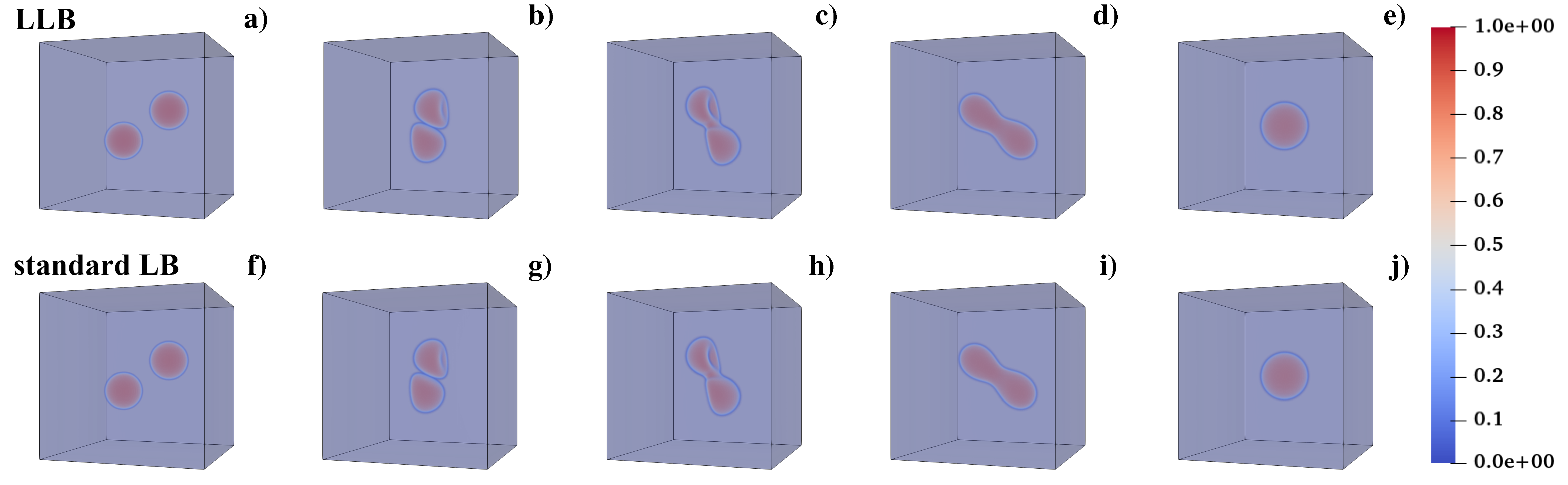
Figure 12: A sequence of an off-axis collision between two fluid droplets simulated using the LLB scheme without populations (a)-(e) and a standard LB scheme with populations (f)-(j). The centers of mass are initially positioned at a distance where the droplets’ mutual interaction is minimal. The droplets, starting as perfect spheres [(a)-(f)], acquire a bullet-like shape as they collide (b), (c) and (g), (h). They then separate (d)-(i) and regain a spherical shape once sufficiently far apart (e)-(j). There is no significant difference between the two methods. The color map shows the density field values, which range from 0 to 1. Adapted with permission from Ref. Tiribocchi et al. (2023c).

We conclude this section by noting that, over the last two decades, several examples of moment-based models have been published, such as the CPU-based one presented in Ref.Argentini et al. (2004) and more sophisticated releases implemented on GPU computers Ferrari et al. (2023); Gounley et al. (2021); Vardhan et al. (2019), where ad-hoc memory layouts are adopted for the hydrodynamics array to capitalize the full memory bandwidth of multi-GPU clusters Ferrari et al. (2023). These techniques have been shown to enhance data continuity, reducing the impact of memory-bound dependence on the implementation Bader (2012) with benefits in terms of computational performance. As a concrete example, Ferrari et al. Ferrari et al. (2023) measured a peak of 10.5 GLUPS on a single GPU NVIDIA A100 PCIe with 40GB RAM adopting a z-curve memory layout for a single component regularized-LB model with an increase of about 20% compared to what observed by Lehmann et al. Lehmann et al. (2022) for a single component BGK-LB model at the same floating point precision.

V Selected applications

In this section, we focus on specific applications which have mostly benefited from the LB approaches and where this method is currently playing a game-changing role, meaning by this that the computational modeling of these applications would have been more demanding, if possible at all, than other methods. We refer primarily to a variety of droplet motions in microfluidic devices, the rheology of confined dense emulsions and other complex phenomena which may lay the ground for a new class of droplet-based materials. More specifically, we identify the following five instances where, we believe, the LB method has shown a major impact: soft flowing crystals, soft granular media, dense emulsions under thermal flows, hierarchical multiple emulsions, active gel droplets in highly confined environments (such as pore-sized constrictions) and extreme flow simulations modeling macroscopic biological entities, such as deep-sea sponges.

V.1 Soft flowing crystals

We initially consider the case of fluid droplets flowing in a microfluidic channel, a system simulated using a color-gradient LB incorporating near-contact interactions, as described in section III.3.1 Montessori et al. (2019b, 2020). Such droplets are usually produced in flow-focusing devices through an emulsification process, in which their generation follows from the periodic pinch-off of the liquid jet of the dispersed phase by the stream of the continuous phase through a small orifice separating the inlet and the outlet chambers Marmottant and Raven (2009); Raven and Marmottant (2009); Garstecki et al. (2004). This emulsion is stabilized by dispersing surfactant molecules preventing coalescence. A sketch of the geometry used in our simulations and the droplet arrangement observed in the channel are shown in Fig.3. These devices are particularly suited for the design of highly monodisperse droplets which are of relevance, for example, for the assembly of droplet-based soft templates with a well-defined structure Nan et al. (2024); Xu et al. (2005); Costantini et al. (2014).

Typical examples of ordered soft materials are soft flowing crystal (also termed as microfluidic crystals Marmottant and Raven (2009)), where monodisperse fluid droplets added in a self-repeating way are found to self-assemble in regular patterns, closely resembling the hexagonal order of solids. In simulations, droplet formation can be controlled by tuning the ratio of dispersed-to-continuous inlet flow, defined as $\chi=u_{d}/2u_{c}$ (where $u_{d}$ and $u_{c}$ are the speed of dispersed and continuous phases) and the dimensionless near-contact number ${\cal N}_{c}=A\Delta x/\sigma$ (see also Eq.42). Here, $A$ is a constant setting the magnitude of the repulsive force and $\Delta x$ is the minimum distance between two interfaces in close contact, generally ranging from $10$ to $100$ nanometers. If ${\cal N}_{c}\ll 1$ droplets coalesce, otherwise repulsive near-contact forces prevail and droplet merging is inhibited.

In Fig.13a-d we show a variety of crystal-like structures confined in microfluidic channels obtained from LB simulations and experiments of air bubbles in water Marmottant and Raven (2009); Raven and Marmottant (2009). Despite the difference in density ratio, the two systems exhibit very similar features. In particular, the emulsion displays a number of phases comprising a three-row configuration (hex-three, (a)), where a regular array of droplets accommodates along three parallel rows, two two-row ones (wet (b) and dry (c) hex-two) and a single-row structure (hex-one, (d)), in which highly-packed droplets arrange in a neat line. Besides being capable of describing the formation and ordering properties of fluid emulsions under confinement, LB simulations also capture the behavior of the flow rate curve and, remarkably, the non-trivial transition from the hex-two to the hex-one regime (see Fig.13e,f). Indeed, experiments show that, for a gas-liquid foam, $Q_{g}\propto P_{g}^{\alpha}$, where $Q_{g}$ and $P_{g}$ are flow rate and pressure of the gas, and $\alpha=3/2$ for small values of $P_{g}$ Marmottant and Raven (2009). On the contrary, for higher values of $P_{g}$, $Q_{g}$ displays a sharp decrease due to the augmented friction of the interfaces with the walls, an effect signaling the transition to the hex-one phase (Fig.13e). These results are reproduced, with high accuracy, by LB simulations of fluid emulsions, where the flow rate $Q_{d}$ of the dispersed phase follows a power law of $\phi$ (which plays the same role as the gas pressure) with an almost equal value of the exponent. In agreement with experiments, simulations also show that the transition from the hex-two to the hex-one phase is marked by a T1 event Graner et al. (2008); Marmottant et al. (2008); Weaire and Hutzler (2001) (corresponding to a topological rearrangement of neighboring droplets) and a transition front, separating the two phases and comoving with the flowing emulsion.

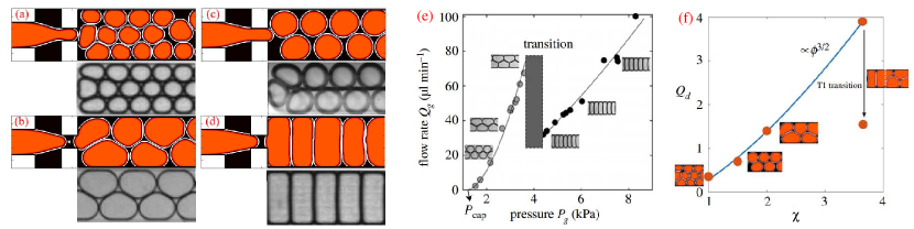
Figure 13: (a)-(d) Simulated (top rows) and experimental (bottom rows) structures of flowing droplets in a microfluidic channel for $\chi=1$ (a) (hex-three), $\chi=1.5$ (b) (wet hex-two), $\chi=2$ (c) (dry hex-two) and $\chi=3.6$ (d) (hex-one). Here $\chi=u_{d}/2u_{c}$, being $u_{d}$ and $u_{c}$ the speed of dispersed and continuous phases. (e)-(f) Flow curves of experimental Marmottant and Raven (2009) and simulated Montessori et al. (2020) soft flowing crystals. In (e) $P_{g}$ and $Q_{g}$ are the gas pressure and gas flow rate. For values of $P_{g}$ lower than $4$kPa, the mixture is in the hex-two regime, where the flow rate scales as $Q_{g}\propto P^{1/\alpha}$ and $\alpha\simeq 2/3$. At $P_{g}\simeq 4$kPa, $Q_{g}$ displays a sharp transition towards the hex-one regime. In (f) $Q_{d}=\nu V_{d}$ is the flow rate of the dispersed phase, where $\nu$ is the frequency of droplet generation and $V_{d}$ is the volume of the generated droplet. The flow rate follows a power law for low values of $\chi$, while for $\chi\simeq 3.5$ a decrease of $Q_{d}$ marks the transition from the hex-two to the hex-one phase. The transition front is indicated by a white dotted line in the top inset. The figures are reproduced with permission from Ref.Montessori et al. (2019b, 2020).

LB simulations of microflows have also been capable of describing morphology and assembly of droplets flowing in convergent and divergent channels Montessori et al. (2019b); Gai et al. (2022); Y. et al. (2016); Luo et al. (2021); Montessori et al. (2021a, b), as the ones shown in Fig.14. More specifically, numerical results suggest that the degree of monodispersity and the arrangement of a confined dense emulsion can be controlled by properly tuning the opening angle ($\alpha$) of a divergent channel and Capillary number ($Ca$) (see Fig.14). Indeed, while for $\alpha\lesssim 40^{\circ}$ the emulsion is generally monodisperse (Fig.14a) regardless of the values of $Ca$, for $45^{\circ}\lesssim\alpha\lesssim 60^{\circ}$ the generated emulsion becomes bidisperse, an effect amplified at high values of $Ca$ (see Fig.14b,c) because breakup events are more likely to occur. The mechanics leading to droplet rupture is highlighted in Fig.14e-n. The orange droplet gradually stretches because of the combined effect of i) the normal force of the incoming droplet (yellow), ii) the extensional force of the channel expansion, and iii) the downstream droplet (red) acting as a ”wall”. Once a critical elongation is overcome, the orange droplet fragments produce two smaller droplets moving towards the upper and lower part of the channel. Then the process self-repeats; the yellow droplet fills the gap left by the orange one and acts as a ”wall” droplet, while a newly generated one will stretch and finally break following a protocol similar to the orange one. Interestingly, further increasing $\alpha$ restores a monodisperse emulsion, once again regardless of the values of $Ca$ (see Fig.14d). This counter-intuitive behavior is due to the fast recovery of the circular shape in the main channel because of larger aperture angles. Such an expansion favors the transversal displacement of the incoming droplet, thus suppressing the squeezing effect. Note finally that, for all geometries considered, increasing $Ca$ generally leads to the formation of a foamy-like emulsion; this is because, in this regime, morphological deformations become easier and, once breakups occur, the resulting smaller droplets fill the voids among neighboring ones.

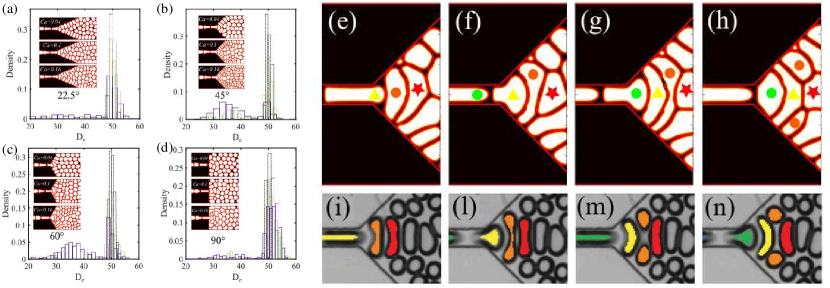
Figure 14: (a)-(d). Droplet assembly in diverging channels of opening angle $\alpha$ equal to $22.5^{\circ}$ (a), $45^{\circ}$ (b), $60^{\circ}$ (c), $90^{\circ}$ (d) and three different values of Ca. The histograms show the distribution of droplet diameters $D_{e}$ for $Ca=0.04$ (dashed line), $Ca=0.1$ (dotted line) $Ca=0.16$ (full line). Note that, for $45^{\circ}\lesssim\alpha\lesssim 60^{\circ}$, the emulsion displays a bidisperse structure (disordered), while for values out of that range, the emulsion is essentially monodisperse (ordered). (e)-(n). Pinch-off mechanism from LB simulations (e-h) and experiments (i-n) at $Ca\simeq 0.08$ and $\alpha=45^{\circ}$. The split of the orange droplet is caused by the confining effect of the yellow droplet (the ”pincher”) and the red one (the ”wall”). The figure is reproduced with permission from Ref.Montessori et al. (2021b).

A reliable description of foamy flows can also be obtained by using other numerical techniques, such as volume-of-fluids methods, which have recently demonstrated the capability of capturing the formation and ordering of air bubbles dispersed in water (thus high-density ratio mixtures) and flowing within microchannels Karnakov et al. (2022). However, these methods have so far shown limited applicability to describe higher complex systems where close-packed deformable drops (or bubbles) are encapsulated within a soft shell, i.e. a soft granular medium with a double emulsion structure. In the next section, we discuss some recent advances in understanding the properties of these systems using LB simulations.

V.2 Soft granular media

Soft granular materials abound in nature, with examples ranging from foams and dense emulsions Datta et al. (2014); Montessori et al. (2021c); Guzowski and Garstecki (2015); Bogdan et al. (2022); Adams et al. (2012); Utada et al. (2005); Abate and Weitz (2009) to biological tissues Weaire and Hutzler (2001); Cohen-Addad et al. (2013); Douezan et al. (2011). The simplest realization in the lab consists of a high volume fraction of immiscible droplets encapsulated within a soft shell containing an oil phase, in turn, immersed in a bulk aqueous phase.

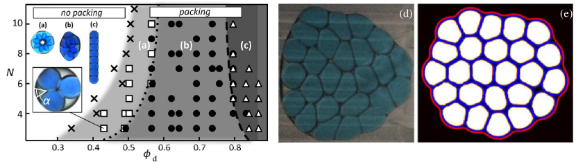
Figure 15: Left panel, (a)-(c). Phase diagram of a soft granular medium, where $N$ is the number of cores and $\phi_{d}$ is the volume fraction they occupy. Insets (a), (b) and (c) represent three possible configurations, where (a) indicates weakly deformed shells, (b) highly deformed ones, and (c) a linear chain. Right panel, (d)-(e). Experimental realization of a soft granular medium (d) formulated using three Newtonian fluids. A result obtained from LB simulations (e) using three-component fluid, i.e. the dispersed phase (white droplets), the lubricating phase (blue), and an external fluid (black). Copyright granted under the https://creativecommons.org/licenses/by/4.0/ CC 4.0 International license and https://creativecommons.org/licenses/by/3.0/ CC 3.0 license respectively. No changes were made from the original figure from Ref.Montessori et al. (2021c); Guzowski and Garstecki (2015).

Recent experiments have shown that these materials exhibit a complex phase diagram, where multiple topologies can be obtained by varying the volume fraction $\phi_{d}$ and the number $N$ of the internal droplets (Fig.15a-c). Indeed, one can identify a region where the packing mildly deforms the emulsion (for $\phi\simeq 0.5$) alongside a wider phase where the emulsion shows a significant departure from the spherical shape (for $0.6\lesssim\phi\lesssim 0.8$). For higher values of $\phi_{d}$, the internal droplets (also termed as cores) arrange into a stable linear chain encapsulated within an elongated shell. Such a picture decisively depends on the grain structure as well as on the deformability of the cores, features controlling the formation of highly packed structures with a volume fraction typically well above the close packing limit of hard spheres.

A far more intriguing scenario is observed in the presence of external flows, where the combination of granularity and deformability leads to complex multiscale dynamics, including plasticity Marmottant and Graner (2013); Dollet et al. (2015), memory effects Jiang et al. (1999); Wang et al. (2013), yield-stress transitions Lulli et al. (2018); Bonn et al. (2017) and glassy dynamics Goyon and Bocquet (2010); Sbragaglia et al. (2012). If driven through narrow geometries, such as a constriction of a microchannel, these materials are usually subject to dramatic morphological transitions which may yield events like the rupture of the shell or the coalescence of the inner droplets, eventually jeopardizing the stability of the emulsion Montessori et al. (2021a, c); Rosenfeld et al. (2014a). Hence, a deep understanding of the fluid-structure interactions governing the physics of these systems is fundamental for ameliorating their mechanical properties, also considering their relevance to biology as models to investigate the behavior of cell clusters crossing physiological constrictions Y. et al. (2016); Au et al. (2016).

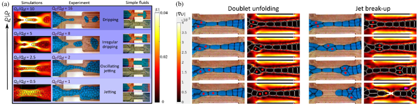
Figure 16: (a) Dynamic patterns observed in a soft granular medium by varying $Q_{c}/Q_{d}$. The medium consists of water-in-oil emulsion surrounded by a further immiscible phase (fluorinated fluid). The left column shows simulation results, the central one shows the corresponding experiments and the right one refers to a water (blue)-oil (transparent) mixture. The color bar refers to the fluid velocity in simulations. (b) Mechanism leading to the jet breakup. If a doublet enters the narrowing and unfolds, the droplet chain is stabilized. Otherwise, high velocity gradients in the surrounding of the doubled (see the pink arrow) destabilize the chain. Copyright granted under the https://creativecommons.org/licenses/by/4.0/ CC 4.0 International license. No changes were made from the original figure from Ref.Bogdan et al. (2022).

LB simulations prove, once again, instrumental to capture crucial aspects of the physics of such systems. In Fig.16a, for example, a series of experiments about the formation of dynamic modes of a confined granular medium (a densely packed monodisperse emulsion focused by an external immiscible phase through an orifice) are presented, while the numerical simulations are performed using the color gradient LB described in section III.3.1. Upon varying the flow ratio $Q_{c}/Q_{d}$ between the continuous and the dispersed phases, both experiments and simulations show that one can distinguish four modes, consisting of (i) a thick, weakly oscillating jetting phase, (ii) a thin, strongly oscillating jet with occasional breakups, (iii) an irregular dripping phase of polydisperse double emulsions, and (iv) a regular dripping phase of monodisperse double emulsions. In stark contrast, Newtonian liquids (such as water in oil mixture) only show two primary modes, i.e. dripping and jetting, although other regimes have been reported Utada et al. (2007).

Besides describing at a high level of accuracy (an almost one-to-one mapping to experiments) these complex structures, LB simulations also unveil the mechanism causing the jet breakup and leading to the dripping phase, as shown in Fig.16b. This is essentially based on the droplet rearrangement upon entering the constriction and on the magnitude of the associated velocity gradients. Indeed, when a doublet (i.e. a pair of droplets) enters the narrowing, the surrounding continuous phase accelerates to conserve the flux. If the doublet unfolds into a chain, the velocity gradients remain weak and the chain is stabilized; on the contrary, if the doublet survives, increasing velocity gradients around it destabilize the jet leading to the breakup.

These results suggest that the color gradient LB augmented with near-contact forces provides a robust numerical platform to study the hydrodynamics of different examples of confined soft granular media, ranging from soft flowing crystal to densely packed aggregates structured in a double emulsion configuration. Recently, it has been also shown that some aspects of the physics of dense emulsions can be efficiently described by using the Shan-Chen approach described in section III.3.3. In the next section, we discuss the dynamics of a dense emulsion subject to thermal convection simulated by this method.

V.3 Dense emulsion under thermal flows

The Shan-Chen approach has been extensively used in applications, such as soft glassy systems Benzi et al. (2009, 2014); Sbragaglia et al. (2012) and coarsening dynamics Pelusi et al. (2019); Tiribocchi et al. (2019), where heat transfer is generally neglected. However, heat transfer can be relevant in a variety of contexts, ranging from polymeric mixtures Voit et al. (2005) and binary fluids Gonnella et al. (2010) to the convective motion of magma Stein and Spera (1992). In Refs.Pelusi et al. (2022, 2021), Pelusi and coworkers have extended the applicability of the Shan-Chen approach to the study of dense emulsions subject to thermal convection, where the temperature field is coupled with the momentum equation of the emulsion. More specifically, the dynamics of the scalar temperature $T$ is simulated by introducing an auxiliary set of distribution functions governed by a single relaxation time lattice Boltzmann equation

$$g_{i}({\bf x}+{\bf c}_{i}\Delta t,t+\Delta t)-g_{i}({\bf x},t)=-\frac{1}{\tau_{g}}(g_{i}({\bf x},t)-g^{eq}_{i}({\bf x},t)),$$ (82)

where $T({\bf x},t)=\sum_{i}g_{i}({\bf x},t)$ and $g_{i}^{eq}$ is the usual second-order expansion in the fluid velocity of the Maxwell-Boltzmann distribution. In the long-wavelength limit, Eq.(82) approximates an advection-diffusion equation of the temperature

$$D_{t}T=\kappa_{T}\nabla^{2}T,$$ (83)

where $D_{t}=\partial/\partial_{t}+{\bf u}\cdot\nabla$ is the material derivative and $\kappa_{T}=c_{s}^{2}(\tau_{g}-1/2)$ is the thermal conductivity.

A typical simulation setup is shown in Fig.17a, where a non-coalescing dense emulsion, initially structured as a honeycomb, is confined between two parallel plates on a two-dimensional lattice (the horizontal direction is periodic), while gravity acts along the wall-to-wall direction. At the boundaries, no-slip conditions are set for the velocity and Dirichlet conditions are imposed for the temperature. The emulsion is then relaxed and stabilized to a state taken as a starting configuration before the convection (Fig.17b). A typical thermal effect is shown in Fig.17c, where convective rolls emerge as the emulsion is heated from below and cooled from above (as in a Rayleigh-Bénard convection Rayleigh (1916); Bénard (1900); Lohse and Xia (2010)). In these simulations, $Ca$ is kept lower than $0.01$ (thus shape deformations are negligible) and $Re$ lower than $100$.

A systematic investigation on the effect produced by varying droplet concentrations, from very dilute regimes (Newtonian emulsion) to dense ones, has been carried on in Ref.Pelusi et al. (2021). It has been shown, for example, that, at increasing concentration, the Nusselt number (measuring the heat transport efficiency) displays significant fluctuations around the mean value, in stark contrast with the dilute case where the fluctuations turn very weak and the transition to convection is accompanied by a steady flow. These results show that, alongside the near-contact LB method, the Shan-Chen approach can provide a further valuable platform to study the physics of confined dense emulsions where coalescence is inhibited. It would be of interest to extend these simulations to three dimensions where out-of-plane components of the fluid velocity are likely to play a non-trivial role.

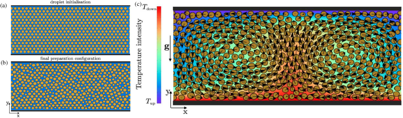
Figure 17: (a) Initial setup of a dense emulsion arranged as a honeycomb structure. (b) Relaxed configuration, taken as a starting point for the convection simulation. In these configurations, the temperature does not affect the fluid flow. (c) Instantaneous configuration of a Rayleigh-Bénard convection in a cell once the emulsion is heated from below. Black arrows indicate the direction of the droplet and the color map represents the values of the temperature. Finally, ${\bf g}$ is the gravitational acceleration. The figure is reproduced with permission from Ref.Pelusi et al. (2022).

V.4 Flowing hierarchical emulsions

An alternative numerical strategy to study the hydrodynamics of dense emulsions with hierarchical structure (a broad class including soft granular media as well) is based on the hybrid free energy LB method using a multiphase field approach (see section III.3.2). In this model, a set of scalar field $\phi_{n}({\bf x},t)$, $n=1,...,N$ describes the density of each droplet (being $N$ the total number of droplets) and the vector field ${\bf u}$ accounts for the global fluid velocity. The dynamics of the scalar fields is governed by a set of advection-diffusion equations of the form of Eq.(52), while the velocity field obeys the Navier-Stokes equation whose stress tensor includes forcing terms associated to each phase. Over the last few years this approach, often combined with LB methods, has been used to simulate systems such as deformable droplets in microchannels Foglino et al. (2017, 2018); Negro et al. (2023); Tiribocchi et al. (2020a) and cell monolayers displaying liquid crystal features Loewe et al. (2020); Mueller et al. (2019); Armengol-Collado et al. (2023). In this subsection, we discuss its use in the context of multiple emulsions flowing within a microfluidic channel, as presented in Ref.Tiribocchi et al. (2021c).

Unlike the examples shown in subsections V.1 and V.2 focused on droplet production, here the interest is in the long-term behavior of these systems. The emulsion is initialized by defining a set of phase fields $\phi_{n}$ which relaxes towards equilibrium for a relatively short simulation time (see Fig.18, top row). At the boundaries, no-slip conditions are set for the fluid velocity and neutral wetting for the phase fields, although no wetting would essentially lead to similar results provided that the interaction between droplets and walls is negligible. Once mechanical equilibrium is attained, a constant pressure gradient is applied across the longitudinal direction of the channel. As time progresses, a large variety of non-equilibrium states is found, ranging from long-lived ones at low values of area fraction of the cores to short-lived ones at higher values. In the former regime, the cores are found to display a correlated planetary-like motion, in which they cease each other while remaining confined either in the upper or lower part of the emulsion for long periods of time. In the latter one, the increase of area fraction triggers collisions and multiple crossings between the two regions, finally leading to a chaotic-like dynamics.

In the bottom row of Fig.18, we show a selection of these steady states. The first scenario is found at values of core area fraction lower than $0.35$ (corresponding to $N=1,2,3$), where the cores exhibit the periodic dynamics confined in a portion of the emulsion, while the second one, in which crossing events occur, appears at higher values (corresponding to $N=4,5,6$) up to approximately $0.5$. This complex behavior is decisively driven by the internal vorticity, consisting of two counter-rotating vortices within the external droplet. If the core area fraction is below $0.35$, the vortex structure remains essentially unaltered (such as the one shown in Fig.18m), whereas it turns chaotic for higher values, due to the non-trivial coupling of the fluid velocity with the interfaces of the cores.

The existence of these steady states is generally guaranteed as long as the inner suspension is sufficiently monodisperse and the capillary number is lower than $1$. For highly polydisperse mixtures, for example, the cores have been found to either get stuck at the front end of the emulsion or confine, separately, in the upper and lower region. Also, increasing the capillary number of the external interface induces large shape deformations which, in turn, squeeze the fluid vortices finally hindering the rotational motion Tiribocchi et al. (2021a). We finally note that a persistent rotating motion could also be produced under Couette flow, where two confining walls move along opposite directions Tiribocchi et al. (2020a, 2021b, b). Unlike the previous case, the motion would be triggered by a single vortex confined within the droplet and resulting from the sheared structure of the flow.

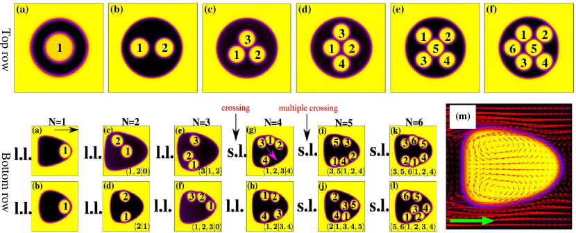
Figure 18: Top row: Equilibrium configurations of a double emulsion (a), a two-core (b), a three-core (c), a four-core (d), a five-core (e) and a six-core (f) emulsion. A set of scalar fields $\phi_{n}$ is associated to each droplet. Bottom row: (a)-(l) The figures show a list of non-equilibrium steady states of multiple emulsions under a pressure-driven flow. If the area fraction occupied by the cores is lower than $\sim 0.35$, the states are long-lived (l.l., corresponding to $N=1$, $N=2$, and $N=3$). The cores are either stuck at the front end or remain confined in the upper/lower part of the emulsion, often displaying a periodic motion along circular trajectories. If the area fraction is higher, the states turn to short-lived (s.l., corresponding to $N=4$, $N=5$, and $N=6$), and multiple crossings from one region towards the other one are observed. Here, Reynolds numbers range from $\sim 1$ to $\sim 3$ and Capillary numbers from $\sim 0.35$ to $\sim 0.85$. The dotted black arrow indicates the direction of motion of the emulsion, while the magenta one the direction of a crossing. In each snapshot, the steady states are classified in terms of an analogy with the occupation number formalism. (m) Typical double-vortex structure of the velocity field computed in the reference frame of a droplet subject to a pressure-driven flow. The color map ranges from $0$ to $2$ and accounts for the values of the phase fields. Copyright granted under the https://creativecommons.org/licenses/by/4.0/ CC 4.0 International license. No changes were made from the original figure from Ref.Tiribocchi et al. (2021c).

Production and dynamics of a double emulsion in a planar flow focusing can be also described using a ternary free-energy lattice Boltzmann Wöhrwag et al. (2018); Wang et al. (2020) where, unlike the hybrid version previously mentioned, the Navier-Stokes equation and the two equations of the order parameters (i.e. the densities of the inner and outer droplets) are solved by means of three different sets of distribution functions, essentially one for each hydrodynamic field. A selection of flow regimes obtained using this method for different values of Capillary numbers are shown in Fig.19, where a significant match with experiments is also reported. One can identify, for example, the two-step formation regime, (a1-b1), the one-step one (a2-b2), the decussate regime with one empty droplet (a3-b3), and the decussate regime with two empty droplets (a4-b4).

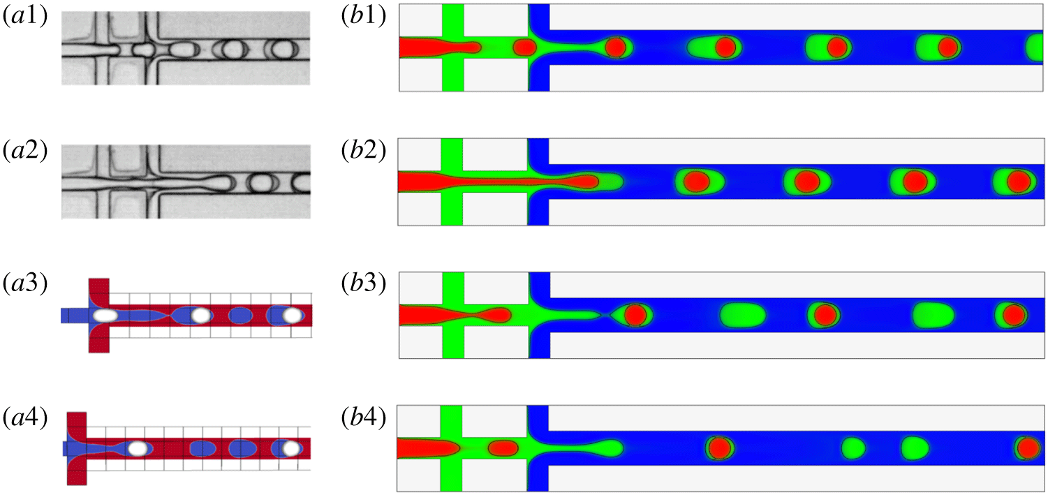
Figure 19: Experimental flow regimes reported in experimental Ref.Abate et al. (2011) (a1,a2) and simulation Azarmanesh et al. (2016) (a3-a4). Simulations from Ref.Wang et al. (2020) (b1-b4). Capillary numbers reported in Ref.Wang et al. (2020) are: (b1) $Ca_{i}=0.012$, $Ca_{m}=0.011$ and $Ca_{o}=0.035$; (b2) $Ca_{i}=0.018$, $Ca_{m}=0.011$ and $Ca_{o}=0.035$; (b3) $Ca_{i}=0.008$, $Ca_{m}=0.011$ and $Ca_{o}=0.035$; (b4) $Ca_{i}=0.008$, $Ca_{m}=0.011$ and $Ca_{o}=0.065$, where the subscripts $i$, $m$ and $o$ indicate inner, medium and outer fluid, respectively. Copyright granted under the https://creativecommons.org/licenses/by/4.0/ CC 4.0 International license. No changes were made from the original figure from Ref.Wang et al. (2020)

The method discussed in this subsection has been also adopted to describe active fluids where, unlike the previous cases, spontaneous flows emerge at a mesoscale level as a result of the action of smaller units that self-propel Marchetti et al. (2013); Ramaswamy (2010). Typical examples are dense suspensions of bacteria dispersed in a fluid, protein networks in living cells, and artificial microswimmers. In the next section, we present a recent application of the lattice Boltzmann method to the dynamics of an active gel droplet migrating through a microfluidic constriction.

V.5 Migration of active droplets through constrictions

Active fluid droplets are a class of bio-mimetic self-propelled systems whose autonomous motion is powered by an active gel often located within the dropletSanchez et al. (2012); Michelin (2023); Seemann et al. (2016); Guillamat et al. (2018). Experimentally realized active droplets typically consist of a water-in-oil emulsion containing, for instance, a dispersion of microtubules and kinesin Sanchez et al. (2012); Guillamat et al. (2018); Doostmohammadi et al. (2018); Ruske and Yeomans (2021); De Magistris et al. (2014) or an actomyosin solution Poincloux et al. (2011); Tjhung et al. (2012, 2017); Sakamoto et al. (2022). Microtubules plus kinesin is an example of extensile material, in which the surrounding fluid is pushed away from the center of mass of the particle, whereas the opposite holds for actomyosin, belonging to contractile systems. These active droplets hold interest as model tools for studying some aspects of the dynamics of living cells Ziebert and Aranson (2016), such as swimming Tjhung et al. (2012), crawling Tjhung et al. (2015) and spontaneous division Giomi and DeSimone (2014), as well as for the design of biomimetic soft materials of relevance in pharmaceutics, for drug delivery Li et al. (2018), and material science, for tissue engineering Saw et al. (2017).

The theoretical framework capturing the behavior of these systems at a continuum level (described in Section III.3.2) combined with the free-energy lattice Boltzmann has been particularly fruitful in simulating the dynamics of active fluid droplets in a highly diluted regime and under confinement. In Fig.20A-B (left panel), we show, for example, the structures of the polar and velocity field of a contractile (i.e. $\zeta<0$) fluid droplet, representing a minimal model of an actomyosin cell extract, in an unbounded medium. The droplet is initialized as a circular region where the polarization vector ${\bf p}$ is uniform and unidirectional. At increasing values of $\zeta$, two regimes can be distinguished: a non-motile one where a four-roll mill flow stretches the droplet longitudinally and a motile one where once $\zeta$ overcomes a critical value, the internal flow acquires a double-vortex pattern propelling the droplet forward. This structure breaks the inversion symmetry of the polar field, leading to an emergent elastic splay and motion along the direction of ${\bf p}$.

A similar theoretical description can be used to study the dynamics of a contractile droplet through constrictions, a phenomenon of relevance in a number of biological processes such as cancer spreading and wound healing Davidson et al. (2015); Au et al. (2016); Cao et al. (2016); Brückner et al. (2019). In Fig.20a-v, we show the migration of a droplet of diameter $D$ through a pore modeled as two static and fluid-free phase fields (the pillars) placed at distance $h$ and glued to opposite flat walls. Although a crude approximation of a realistic constriction, this design allows for a simple implementation of mesoscale effects, such as repulsion and adhesion between the droplet and pillars. Adhesion, in particular, can be included by adding a contribution of the form $\sum_{n,m,n<m}\gamma_{n,m}\nabla\phi_{n}\nabla\phi_{m}$ to the free energy, where $\gamma_{n,m}$ is an adhesion constant between different phase fields.

Importantly, adhesive forces are found to be crucial in enabling the crossing, especially through narrow interstices Tiribocchi et al. (2023d). Indeed, while for large pores (Fig.20a-f, $h/D\simeq 0.8$) the crossing generally occurs if the speed (which is controlled by the activity $\zeta$) is high enough, for smaller pores (Fig.20g-v, $h/D\simeq 0.5$ and $h/D\simeq 0.2$) the sole active stress is not sufficient to enable the process. In this case, the droplet would either get stuck at the pore’s entry or bounce back into the microchannel. Simulations show that, under these conditions, non-uniform adhesive forces (i.e. higher at the entry of the pore and lower at the exit) are necessary for a successful crossing, provided that inertia, surface tension, and adhesion are carefully balanced. Suitable dimensionless numbers assessing the importance of these effects are the adhesion number $A=\gamma_{L}/\gamma_{R}$, which is the ratio between adhesion forces at the entry and the exit of the pore, and the inertia-over-adhesion number $I_{A_{L,R}}=\rho v^{2}R^{2}/\gamma_{L,R}$. For $\lambda\simeq 0.5$, for example, one has $2\lesssim A\lesssim 10$, $I_{A_{R}}\simeq 0.25$ and $0.025\lesssim I_{A_{L}}\lesssim 0.06$. The values of the last two numbers, in particular, mean that inertial forces are weaker than adhesive ones at the entry (L) of the pore to enhance the connection between the droplet and pillars. A lower adhesiveness at the exit (R) allows for an easier detachment from the pore, finally favoring the crossing.

Although this model remains distant from a living cell in many aspects, such as the lack of the nucleus, which represents a limiting factor in the crossing, yet these results may suggest that some features of cell motility can be reasonably captured by minimal mesoscopic models built upon a restricted number of dynamic parameters and hydrodynamic fields.

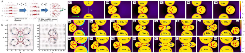
Figure 20: Left panel, (A)-(B). In (A), the figure shows the initial configuration of the active droplet (left), the intermediate non-motile state (middle), and the motile state (right). Red arrows indicate the direction of the polar field, which turns from a uniform orientation at equilibrium to a splay deformation at the steady state. In (B), the figure shows the steady-state velocity fields for the intermediate configuration (left) and the motile one (right). The former consists of a four-roll mill flow, while the latter exhibits two counter-rotating vortices propelling the droplet. Here, red arrows indicate the direction of the velocity field. Right panel, (a)-(v). This panel shows the crossing of an active fluid droplet of diameter $D$ through a constriction of height $h$. In (a)-(f) $h/D\simeq 0.8$, in (g)-(n) $h/D\simeq 0.5$ and in (o)-(v) $h/D\simeq 0.2$. Decreasing the ratio $h/D$ yields larger shape deformations, some closely resembling experimentally observed structures, such as ampule-like (j,k,r,t) and hourglass (s) configurations. For $h/D\lesssim 0.5$, larger adhesive forces (pink layer in (g) and (o)) at the entrance of the pore and weaker ones (cyan layer) at the exit are crucial to favor the crossing. Here, $\gamma_{L}$ and $\gamma_{R}$ indicate the adhesion coefficient at the left and right sides of the pillars, large red arrows highlight splay deformations, and blue ones indicate bend distortions. The color map ranges from $0$ to $2$ and accounts for the values of the phase fields. The left panel is reproduced with permission from PNAS Ref.Tjhung et al. (2012). Copyright granted under the https://creativecommons.org/licenses/by/4.0/ CC 4.0 International license. No changes were made from the original figure from Ref Tiribocchi et al. (2023d).

V.6 Peta-scale simulations of deep-sea sponges

We conclude this section with a discussion on a recent application where the LB method is adopted to study the fluid dynamics of the deep-sea glass sponge Euplectella aspergillum Falcucci et al. (2021), a soft living organism that, besides representing a fascinating example of life under extreme conditions (at depth of $100$-$1000$ m in the Pacific Ocean and Antarctic area with no ambient sunlight), displays intriguing structural properties due to the trabecular arrangement of its skeletal system Monn et al. (2015); Fernandes et al. (2020).

The interest of this study lies in the fact that, despite the use of a single-component interface-free lattice Boltzmann (thus its easiest realization), the detailed three-dimensional reconstruction of the skeleton of the sponge and the computation of the fluid flow in which this organism is immersed need to leverage two of the main advantages of the method, namely the excellent scalability on parallel architectures and the capability of handling complex geometries. Indeed, to reproduce the sponge’s living conditions, the simulations feature over fifty billion grid points spanning approximately four spatial decades, while a complex mesh structure is used to simulate the skeleton.

In Fig.21, we show a simulation of the sponge immersed in a hydrodynamic flow at $Re\simeq 2000$, where $Re=uD/\nu$, being $u$ the water velocity, $\nu$ is its viscosity and $D$ is the sponge diameter at the top section. The sponge structure comprises an anchoring bulb, a section connecting the bulb to the body, the main body and the final sieve plate located at the top. The body, in particular, is simulated using two intersecting patterns of lattices, the first composed of filaments orthogonally crossing each other and the second made by smaller ligaments placed at $45^{\circ}$ with respect to the first one. The resulting cylindrical structure finally bends into a cone connecting with the anchoring bulb. Also, no-slip conditions are imposed at the internal boundaries of the sponge and at the seafloor.

The simulations show, for example, that a considerable decrease in the flow speed occurs inside the sponge’s body (where vortices are formed) and downstream of the organisms, while intermittent fluid patterns emerge several diameters further away. These features are supposed to play a role in feeding through a selection mechanism where nutrients are absorbed in the sponge chambers and inorganic particles are discarded. Also, at $Re>100$ intermittency patterns are delayed, an effect that reduces the stress and potentially enhances the mechanical stability of the sponge. It has also been noted that the presence of the sponge’s tissue (neglected in these simulations) could impact the structure of the fluid flow because the tissue may form a barrier with low permeability over the sponge wall Leys et al. (2022). These conditions could be partially reproduced by modeling the sponge as a porous medium with an effective resistance to the flow, although additional experiments and empirical data would be needed to test more complex models.

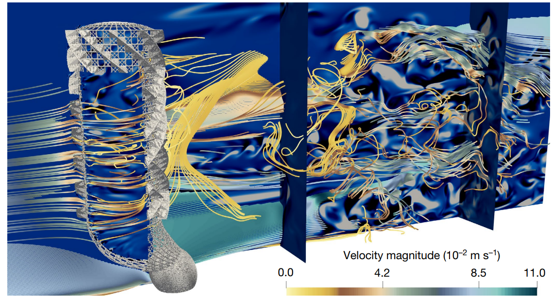
Figure 21: Simulation of a deep-sea sponge immersed in a hydrodynamic flow at $Re\simeq 2000$, where contours of helicity ${\cal H}$ (defined as ${\cal H}={\bf u}\cdot{\bm{\omega}}$, where ${\bm{\omega}}$ is the vorticity) and streaklines of the flow are shown. The figure is reproduced with permission from Ref.Falcucci et al. (2021).

V.7 From applications to engineering design

The set of selected applications presented above is meant to convey the idea of the flexibility and computational efficiency of the LB methods for soft-flowing matter across different regimes of motion. Such flexibility and efficiency are expected to find profitable use in various sectors of industrial and materials design, such as food science, chemical-pharmaceutical (drug design and delivery), tissue engineering and many others. While the details of each and every specific application must necessarily be worked out on a case-by-case basis, in the following we wish to convey the flavor of the potential of computational design in the above sectors based on the LB methods discussed in this review.

For the sake of concreteness, let us refer to a soft material, say a dense emulsion flowing in a box device of height $H=0.1$, width $W=1$ and length $L=10$, all in millimeters. With a lattice spacing $\Delta x=10^{-3}$ (1 micron), the LB simulation consists of $G=10^{2+3+4}=10^{9}$ lattice cells. Such volume contains about a thousand cylindrical droplets of diameter $D=0.1$ mm (100 microns) and height $H$. At a processing speed of $100$ GLUPS, i.e., a hundred billion lattice sites per second, the LB code updates the full box domain a hundred times in a single second of computer time With a timestep of $\Delta t=10^{-9}$ (1 ns), one million timesteps cover $1$ millisecond of physical time. This duration corresponds to $10^{4}$ seconds, namely about three hours of elapsed time over an HPC cluster containing several GPU-based devices Bonaccorso et al. (2022).

At this point, it should be observed that, in one million time steps, the LB populations complete a hundred longitudinal tours along the domain, which sounds very satisfactory. However, the fluid moves much slower than the populations; at a speed of $u=10$ mm/s, in one millisecond, the fluid covers a distance of just ten microns. Hence, the fluid speed must be artificially accelerated by some three orders of magnitude for the fluid to make at least one tour around the device (1 cm long). This is common practice in many simulations, not just LB. The idea is to artificially increase the fluid speed while keeping the relevant dimensionless numbers, in our case the Capillary number $Ca$ and the near-contact number $\mathcal{N}$, unchanged. This can be done by boosting the fluid speed, $u$, the surface tension $\sigma$ and the strength of the near-contact potential $E_{nc}$ by the same factor, so as to keep the ratios $u/\sigma$ and $\alpha/\sigma$ unchanged.

With all this said and done, LB updates a millimeter cube of material consisting of about one thousand droplets at a rate of about ten millisecond/day. The above figures appear consistent with the requirements of engineering design.

VI Whither LB? Outlook and future perspectives

The directions for future LB developments aimed at applications in soft matter research are far beyond the scope of any single review. Therefore, in the following, we restrict to three directions which might bear a special interest in the coming years: quantum nanofluidics, machine learning and prospects for the quantum simulation of soft flowing systems.

VI.1 Towards quantum nanofluidics

The general trend of modern science and engineering towards miniaturization has placed a strong premium towards the study of fluid phenomena at nanometric scales Bocquet and Charlaix (2010); Coquinot et al. (2023); Kavokine et al. (2021); Bocquet (2020). This tendency draws from many technological sources, including biology, biomedical, chemical-pharmaceutical, and energy/environment. Given the vast amount of energy lost on frictional contacts, low contact friction is paramount to the optimal design of most micro and nano-mechanical devices involved in these applications.

According to continuum mechanics, the pressure gradient to push a given mass flow across a channel of diameter $D$ scales like $D^{-4}$. Indeed, the centerline velocity of a Poiseuille flow across a channel of diameter $D$ reads as follows

$$u_{c}=const.\;\frac{\nabla_{x}pD^{2}}{\mu},$$

where $const.$ is a geometry-dependent constant. The mass flow rate, $\dot{M}$, is then obtained by multiplying the centerline speed by a factor proportional to the area of the cross-section, which provides an additional $D^{2}$ contribution, whence the $\nabla_{x}p\sim{\dot{M}}D^{-4}$ dependence. Such relation speaks clearly for the difficulty of pushing flows across miniaturized devices: with all other parameters fixed, a ten-fold decrease in radius demands a ten-thousand fold increase in pressure.

The above scaling derives from the assumption that the fluid molecules in contact with solid walls do not exhibit any net motion, the so called no-slip condition, because the remain trapped in local corrugations of the solid wall. This assumption is no longer valid whenever the size of the channel becomes comparable with the molecular mean free path and, more generally, whenever the fluid-solid molecular interactions cannot be described in terms of simple mechanical collisions.

Whatever the driving mechanism, the onset of a non-zero fluid velocity at the wall (slip flow), $u_{s}\neq 0$, is a much-sought effect, as it turns the hydrodynamic $D^{4}$ barrier into a much more manageable $D^{2}$ dependence. Slip flow is typically quantified in terms of the so called slip length

$$L_{s}=u_{s}/(du/dy)_{w},$$

where $(du/dy)_{w}$ is the velocity gradient at the wall. Under no-slip conditions, $L_{s}$ is of the order of the molecular mean free path, i.e. about 1 nm for water, while suitably treated (geometrically or chemically) walls can reach up to $L_{s}\sim 10\div 100$ nm, which is comparable to the size of the nanodevice, leading to a very substantial decrease of the effective viscosity (roughly speaking a factor $D/L_{s}$).

Achieving large slip lengths involves nano-engineering of fluid-wall interactions such as to prevent fluid molecules from being trapped by nano-corrugations. This is usually pursued by clever geometrical and/or chemical coatings which promote near-wall repulsion between fluid and solid molecules (hydrophobic coating) Kavokine et al. (2021).

However, in recent years, it has been argued and experimentally shown that unanticipated quantum-electro-mechanical phenomena can also lead to spectacular reduction of frictional losses Coquinot et al. (2023); Lizée et al. (2023). For instance, it has been shown that slip flow in carbon nanotubes is largely underestimated by MD simulations, indicating that standard force-field procedures fall short of describing the actual physics of the water-graphene interactions, pointing to a crucial role of electronic degrees of freedom in the solid Kavokine et al. (2022). Interestingly, ab-initio MD, besides being even more unpractical computing-wise, would also fall short of capturing the basics of quantum friction because the electrons in the solid are non-adiabatically coupled to charge fluctuations in the liquid. Therefore, it would be extremely interesting to enrich the LB formalism in such a way as to include quantum interfacial interactions. This is indeed possible by exploiting recent results obtained from quantum non-equilibrium Keldysh analysis of interfacial transport in nanofluids Coquinot et al. (2023). The Keldysh formalism accounts for non-equilibrium quantum transport phenomena, and in this respect, it necessarily involves very elaborate analytical calculations based on advanced and retarded Green functions. The final outcome, though, comes in the form of Langevin-like friction terms which could be easily incorporated within an LB-extended framework. For the sake of concreteness let us refer to the case of a charged ionic liquid, in which charge fluctuations couple to phononic and electronic degrees of freedom in the solid walls. The Keldysh analysis shows that, under suitable geometrical and physical conditions, such interfacial quantum coupling can lead to a reduction of the wall friction, because part of the momentum imparted to solid electrons is recycled back to the liquid, an effect known as ”negative quantum friction” (see Fig.22).

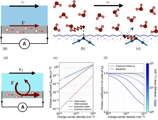
Figure 22: Quantum friction scenarios. (a)-(c) A nanofluidic device exhibiting reduced friction through two different electronic current-drive mechanisms: charged fluctuations in liquid water imparting momentum to the electrons in the solid through Coulomb interactions across the liquid-solid interface (b); electrons in the solid driven by phonons, which are excited by water molecule collisions with the solid molecules (c). (d) A sketch of the electron feedback to the liquid. (d) The electron-phonon friction coefficient as a function of the electron density in the solid for four different scenarios: 2D electron gas (2DEG) coupled to water, 2DEG and phonons coupled to water, Graphene coupled to water, graphene with phonons coupled to water. (f) The overall friction coefficient in graphene as compared to classical friction as a function of the electron density. Copyright granted under the https://creativecommons.org/licenses/by/4.0/ CC 4.0 International license. No changes were made from the original figure from Ref.Coquinot et al. (2023).

Clearly, the inclusion of ”quantum friction” alone is not enough, since, based on the fluctuation-dissipation theorem, quantum fluctuations must be accounted for as well. This is a genuinely new theoretical and computational challenge to LB, since, depending on their energy, the quantum fluctuations may last longer then the LB timestep so that, at variance with standard versions of the fluctuating LB formalism Adhikari et al. (2005); Dünweg et al. (2007), the correlator of the fluctuating force extends beyond a single LB time-step.

In summarizing, one would write three LB equations for the three species in play, hydrons, electrons, and phonons, coupled via screened Coulomb interactions, frictional terms and fluctuating forces. Such a model is best implemented on higher-order lattices so as to capture stronger non-equilibrium effects, stronger fluctuations, and also mitigate spatial non-local effects. It is argued that such Keldysh LB formalism might open an entirely new avenue for the computational design of quantum-controlled low-friction nanodevices.

VI.2 Machine learning

Machine learning (ML) techniques based on artificial neural networks are increasingly employed in microfluidics to perform various tasks, both in experimental and modeling contexts. While in the former case ML is used mainly as an analyzer tool to extract information from images or movies (for instance, to track droplets, bubbles Durve et al. (2023, 2022) and cells Gardner et al. (2022)) or to infer physical quantities, such as shear and deformation rate Ning et al. (2023); Sathyan et al. (2020); Nazar et al. (2023), in the latter ML has recently shown its capability to enhance numerical approaches by improving their accuracy.

Although ML is essentially a data-driven approach, it can be enriched and reinforced with physical foreknowledge of the problem under investigation. This concept is crucial, for example, in Physics-Informed Machine Learning (PIML) techniques Karniadakis et al. (2021), in which data and mathematical models (such as partial differential or integral equations) are integrated and then implemented through neural networks or kernel-based regression networks Wang et al. (2022); Cai et al. (2021). Thus, ML can be used not only as a heuristic tool driven by the statistical inference of large datasets but also as a system that embeds, in the learning process, the physical laws governing a specific data set. In this framework, the artificial neural networks in the ML approach could act as a class of physical-informed models satisfying universal approximation theorems while preserving the physical ingredients and, concurrently, enhancing the overall computational performance.

In the following, however, we shall focus on a specific item: the use of machine learning to enhance the physical accuracy and computational efficiency of LB simulations of complex soft matter flows, including near-contact interactions acting at the scale of a few nanometers.

The task of reaching out to scales of experimental and engineering devices (mm-cm) accounting for near-contact interactions (1-10 nm) entails at least six decades in space and about twice as many in time, resulting in a computational demand which far exceeds the capabilities of current leading-edge near-exascale computers. The standard practice is then to represent and parameterize the effects of the unresolved fine scales on the resolved ones, by suitable coarse-grained models. The success of such strategy hinges heavily on scale separation arguments, meaning by this a sufficiently weak coupling between the fine and coarse scales. Such an assumption may or may not apply depending on the specific problem at hand, hence it is highly desirable to devise non-perturbative methods capable of handling strong-coupling regimes as well. Machine learning is a good candidate to reach this goal, as it can be employed to learn optimal models from experimental or highly-resolved simulation data, without resorting to any weak-coupling assumption, by now a common practice in many areas of computer simulation. In our specific case, we shall focus on two related and yet distinct strategies: i) Learning collision operators for ideal and non-ideal fluids and ii) Learning coarse-grained pseudo-potentials.

VI.2.1 Learning collision operators for ideal fluids

Collision operators for LB simulations of simple fluids can be derived analytically, based on the constraints imposed by the mass-momentum-energy conservation laws. Formally, the mapping from the actual distribution $f$ to the corresponding local equilibrium $f^{eq}$ for the standard single-time BGK collision operator can be written in mode-coupling form as follows:

$$f_{i}^{eq}=A_{ij}f_{j}+B_{ijk}f_{j}f_{k}/\sum_{l}f_{l},$$ (84)

where $A_{ij}=c_{i\alpha}c_{j\alpha}/c_{s}^{2}$ and $B_{ijk}=Q_{i\alpha\beta}c_{j\alpha}c_{k\beta}/c_{s}^{4}$ are constant matrices to be learned by the machine. The denominator at the right-hand side is the fluid density, but since the neural network, in principle, is not aware of it we have left this association unspoken. Formally, the above expression is a highly nonlinear function of the $b$ variables $f_{i}$ ($i=1,...,b$), not only because of the quadratic term $f_{j}f_{k}$ but especially because of the denominator $\sum_{l}f_{l}$, which gives rise to a non-polynomial nonlinearity. The task of learning the multivariate nonlinear expression of Eq.(84) is greatly facilitated by supplementing the neural network with the conservation constraints

$$\sum_{i}f_{i}^{eq}=\sum_{i}f_{i}=\rho,$$ (85)

$$\sum_{i}f_{i}^{eq}c_{i\alpha}=\sum_{i}f_{i}c_{i\alpha}=J_{\alpha}.$$ (86)

With such assistance, the neural network should be able to learn the local equilibrium in its ”mean-field” form, namely

$$f_{i}^{eq}=w_{i}(\rho+{J_{\alpha}}{c_{i\alpha}}+\frac{J_{\alpha}J_{\beta}}{\rho}Q_{i\alpha\beta}),$$ (87)

where the discrete speeds are normalized by the sound speed $c_{s}$. This mean-field form is obviously easier to learn, as it depends only on four independent variables, $\rho$ and $J_{\alpha}$. To the best of our knowledge, this is how machine learning of LB equilibria has been developed so far Lou et al. (2021); Corbetta et al. (2023).

However, many variants of Eq.(87) have been developed in the last decades in order to achieve better stability or incorporate additional macroscale and microscale physics, whose derivation is usually based on informed ad-hoc phenomenological assumptions Succi (2018). The path to these phenomenological models is generally not unique because no systematic procedure is available to derive them from first principles, due to the fact that one is dealing with flowing systems far from equilibrium. This opens up a major scope for machine learning collision operators based on training from experimental data or high-resolution simulations.

Essentially, one is presented with three possible scenarios. The first and most pessimistic one is that the machine fails to learn the existing models for non-ideal fluids, such as Shan-Chen, free-energy or chromodynamic models. The second, less pessimistic, possibility is that the machine learns exactly the same models derived on phenomenological grounds. This would be a success for machine learning but pointless to the purpose of enhancing the LB simulators. The third, and definitely most exciting possibility, is that the machine learns new models which have not been discovered yet. In this case, machine learning would literally teach us new physics, thereby providing a new generation of LB schemes capable of accessing strongly-coupled regimes out of reach for the current LB models for non-ideal fluids.

VI.2.2 Learning generalized collision operators for non-ideal fluids

So much for the general scenario. To date, machine learning for LB is still literally in its infancy, and the work so far has been directed to ideal fluids with no potential energy.

In the field of turbulence, for example, Bedrunka et al. Bedrunka et al. (2021) have presented a PyTorch-based LB code, where a neural collision model (a more accurate version of classical collision models) is trained on a shear layer flow and then applied to a decaying turbulence flow with satisfactory numerical results. Also, convolutional neural network (CNN) and gated recurrent unit neural network (GRU) have been combined with the LB method to reduce computational time and improve the efficiency of turbulent simulations up to Reynolds number of 4000 Zhao et al. (2023).

An intriguing perspective is that offered by the physics-informed neural networks (PINNs). In Ref. Lou et al. (2021), for example, they are used to learn the BGK collision operator of various benchmark flows, such as continuous Taylor-Green flow and rarefied micro-Couette flow. Following a similar footprint, Corbetta et al. Corbetta et al. (2023) have shown that, a neural network architecture combined with suitable physical properties (such as conservation laws and symmetry), allow for a precise reconstruction of collisional operators of lattice Boltzmann and accurate dynamics of standard fluids (such as Taylor-Green vortex and lid-driven cavity flows).

The challenge we wish to briefly discuss in this review is the extension of some of these approaches to the case of collision operators for multiphase and multicomponent flows, including near-contact interactions. A possibility is to develop PINNs incorporating the additional constraints associated with non-ideal momentum-flux tensor inclusive of non-ideal interaction, i.e. the Korteweg tensor. Here we outline the basic steps of the procedure, shortly sketched in Fig.23.

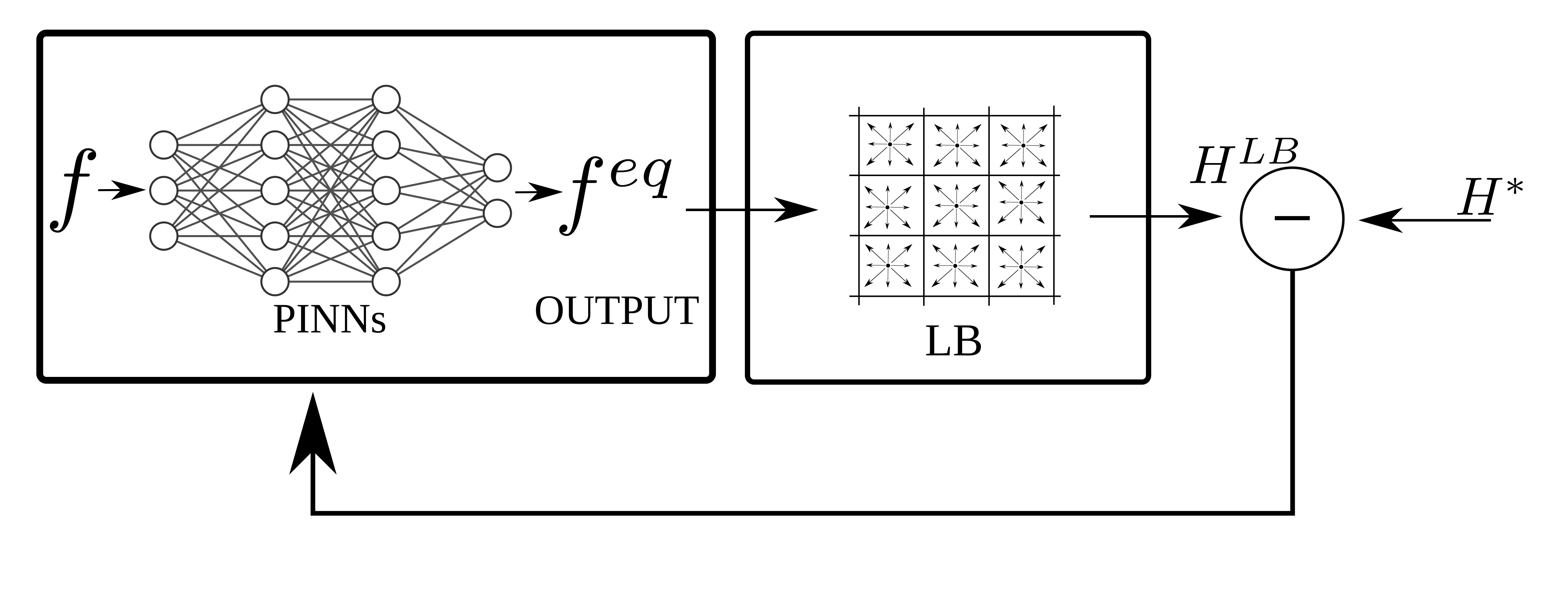
Figure 23: A sketch of the procedure aiming at learning the collision operators of non-ideal fluids. A set of initial distribution functions $f$ trains a neural network which delivers a provisional set of equilibrium distribution functions $f^{eq}$, given by Eq.(88), as output. These ones feed a LB simulation which provides the hydrodynamic observable (such as mass and momentum) to be compared with experimental data. If the match is accepted within a given tolerance, the search ends otherwise the weights $W$ are updated by a gradient-descent method and the algorithm restarts.

Step 1: The NN is presented with the actual value $f_{i}(x)$ of the discrete distributions as an input, and delivers a provisional local equilibrium $f_{i}^{eq}(x)$ as an output, where $x$ denotes the full set of spatial locations. Symbolically,

$$f^{eq}=\sigma^{L}(Wf-b),$$ (88)

where $\sigma^{L}$ denotes the activation function as recursively applied to $L$ hidden layers composing the (deep) neural network, $W$ is the set of weights and $b$ are the associated biases.

Step 2: The LB simulation is run with the provisional set of local equilibria derived in Step 1.

Step 3: The results, namely a set of hydrodynamic observables $H^{LB}$, are compared with the ”truth” $H^{*}$, either experimental data or highly-resolved simulations, to deliver the current value of the loss function

$$\mathcal{L}=dis(H^{LB},H^{*}),$$ (89)

where ”dis” indicates some suitable metric in the space of the functions $H(x)$, for instance the Euclidean distance $\sum_{x}(H^{LB}(x)-H^{*}(x))^{2}$ or similar ones.

Step 4: If the distance $dis(H^{LB},H^{*})$ falls below a given tolerance, the search is stopped. Else, the weights are updated by some form of gradient descent,

$$\delta W=-\alpha\partial\mathcal{L}/\partial W,$$ (90)

and then back to Step 1.

It is known that this search is greatly accelerated by augmenting the loss function with physically inspired constraints. In the case of standard lattice Boltzmann, these are the mass-momentum and momentum-flux constraints. In compact four-dimensional notation, they read as follows:

$$\mathcal{L}_{\mu,\nu}^{PI}=dis(P_{\mu,\nu}^{kin},P_{\mu,\nu}^{eq}),\;\hskip 14.22636pt\mu,\nu=0,d$$ (91)

where we have defined $P_{\mu,\nu}^{kin}=\sum_{i}f_{i}^{eq}c_{i,\mu}c_{i,\nu}$. In the above, we have set $c_{i0}=1$, so that $P_{0,0}^{eq}=\rho$, $P_{0,a}^{eq}=P_{a,0}^{eq}=J_{a}$ and $P_{ab}^{eq}=\rho u_{a}u_{b}+p\delta_{ab}$, where Latin indices running along the spatial dimensions. The loss function associated with these physical constraints is then the sum over the single components $\mu,\nu=0,d$. Such physics-informed loss function is then added to the standard loss function discussed above, as essentially done by previous authors.

For the case of non-ideal fluids, the procedure stays basically the same, with the key proviso that the momentum flux must include the non-ideal component, namely the Korteweg tensor $K_{ab}$, whose kinetic expression is

$$K_{\mu,\nu}^{kin}=\sum_{i}f_{i}^{eq}F_{i,\mu}d_{i,\nu},$$ (92)

where $d_{i0}=0$ and $d_{ia}=c_{ia}\Delta t$ and $F_{ia}$ is the central force acting between two lattice sites $x_{a}$ and $x_{a}+d_{ia}$.

Further on, with near-contact interactions, the Korteweg tensor must be augmented with the near-contact contributions, as explicitly derived in Montessori et al. (2019a). This procedure requires knowledge of the near-contact interactions augmented Korteweg tensor, hence it is expected to recover existing local equilibria or equivalent forcing terms currently used in LB simulations. However, it cannot be ruled out that new generalized equilibria might emerge from the ML procedure discussed above. This would mark a decisive contribution of machine learning to LB simulations of complex soft matter flows. Although we are not aware of any detailed work in this direction, this is a decidedly interesting topic for future research in the field.

VI.2.3 Learning near-contact pseudo-potentials

In Ref.Montessori et al. (2019a) an effective way to incorporate disjoining, near-contact interactions within a chromodynamic LB model for multicomponent flows is presented, which stands as an extreme instance of coarse-graining of the complex physics arising when two fluid interfaces covered by a surfactant come into close contact. Such a picture is typical soft many-body flowing systems, such as dry foams and dense emulsions. As mentioned in Section II, such near-contact interactions aim at condensing a plethora of effects due to the onset of forces arising at nanometric scales, such as electrostatic double-layer, dispersion forces and Casimir-like interactions Derjaguin and Landau (1941); Verwey and Overbeek (1948), within a simplified, one-parameter density functional.

The problems with such a treatment may be summarized through two main points: a) the physical fidelity of the upscaled mathematical formulation is hard to assess a priori and can only be judged ex-facto; b) there is an intrinsic uncertainty related to the choice of the parameters controlling the magnitude of such interaction forces.

The hard way to solve such issues is to systematically ”down-scale” the problem, by studying the details of the interactions through micro-scale techniques, such as molecular dynamics and perhaps even electronic structure methods in case electronic degrees of freedom take an active role Bocquet and Charlaix (2010); Coquinot et al. (2023). The main problem of such a microscopic approach is the lack of computer power to reach out to scales of experimental and engineering design interest, say centimeters. The alternative, top-down approach, is to augment mesoscale forces and pseudo-potentials with additional terms which would retain the essential microphysics within a viable computational framework. Translated into formulas, the near-contact force per unit volume along direction $x_{a}$ is given by:

$$F_{a,nci}=\nabla\cdot\Sigma_{nci}=\nabla\cdot\left(A_{nci}[z;\kappa_{int},u_{rel}]\frac{\nabla\phi}{|\nabla\phi|}\right)\vec{n}\delta_{ab}$$ (93)

where $z$ is the spatial coordinate along the normal $\vec{n}$ of a given interfaces, $u_{rel}$ is the relative velocity and $\kappa_{int}$ is the local curvature of the interface.

By dimensional arguments, one could generically write

$$A(z;\lambda)=\frac{\epsilon(\lambda)}{z^{4}},$$ (94)

where $\epsilon$ is the pseudo-potential to be machine-learned as a function of the ”hydrodynamic” parameters, symbolically denoted by $\lambda$.

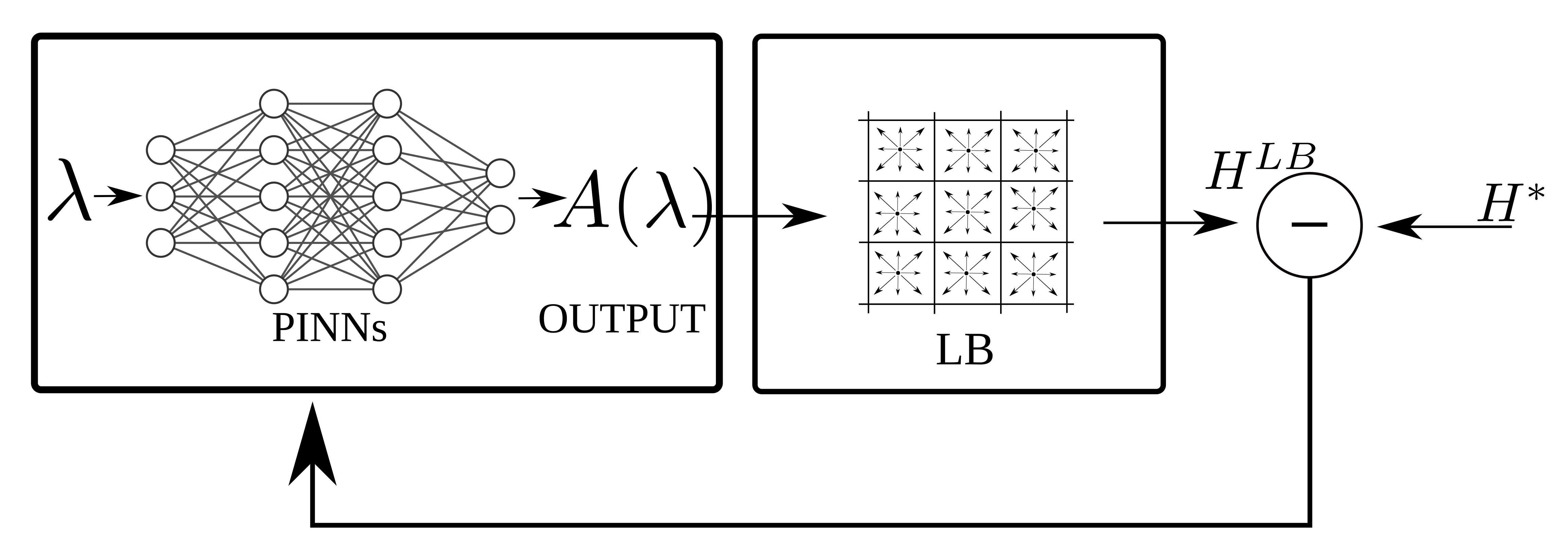
Figure 24: A schematic procedure aiming at learning the functional form of near-contact forces to be included in LB simulations. The training of the PINNs follows the same procedure as the one described in Fig.23, except that the input is a list of parameters $\lambda(x)$ and the output is the function $A(\lambda)$.

The actual procedure would look pretty much like the one discussed earlier, except that the input to the PINN is no longer the actual distribution $f_{i}(x)$ but the set of parameters $\lambda(x)$ which govern the near-contact physics at position $x$ in space (as sketched in Fig.24). Once the PINN finds the functional form of $A$, the near-contact interactions can be introduced within the LB framework through the usual shift of the equilibria or via direct forcing. Then, a LB simulation is run with this temporary form of $A$ to finally produce a list of hydrodynamic variables. Once this step is completed, the subsequent ones proceed following steps 3 and 4 discussed in the previous paragraph.

VI.3 Machine learning for the deformable many-body problem

Yet another application of machine learning we discuss in this review is the derivation of effective equations of motion for soft suspended bodies based on the geometrical parameters of the experimental device.

The first step along this direction is to automatize the identification and tracking of the droplet trajectories. Object tracking constitutes the automated process of identifying and monitoring multiple objects within a series of images. Typically, these tasks are managed by distinct algorithms. The first category encompasses object detection algorithms, which aim to identify multiple objects within a single image. Conversely, the second category, referred to as object trackers, is responsible for assigning unique identity numbers to each detected object, maintaining consistency across successive frames. These persistent unique identifiers serve as the basis for tracking objects across sequential images, thereby generating trajectories.

Object detection algorithms primarily undertake two key tasks: (a) object localization, involving the determination of object positions within an image and the delineation of their boundaries, and (b) classification of the detected objects into predefined categories. Recent years have witnessed significant advancements in the development of object-localization algorithms, such as Region-Based Convolutional Neural Networks (RCNN) Girshick et al. (2014) and their iterations (Fast R-CNN Girshick (2015), Faster R-CNN Ren et al. (2016), Cascade R-CNN Cai and Vasconcelos (2018)), You Only Look Once (YOLO) Redmon et al. (2016) and its subsequent versions Redmon and Farhadi (2018); Bochkovskiy et al. (2020); Jocher (2020); Wang et al. (2023); Jocher et al. (2023), Single Shot MultiBox Detector (SSD) Liu et al. (2016), Single-Shot Refinement Neural Network for Object Detection (RefineDet) Zhang et al. (2018) and Retina-Net Lin et al. (2018), to name a few ones. Conversely, object tracking algorithms are focused on correlating detected objects across consecutive frames and tracking them by learning their distinctive features. Among many examples, DeepSORT Wojke et al. (2017) stands out as one of the most prominent object-tracking algorithms which incorporates deep learning into the tracking process. Interestingly, it has been recently combined with YOLO in order to perform the two aforementioned tasks, i.e. detect and track droplets within experimental setups. This software, named ”DropTrack” Durve et al. (2022, 2023, 2024a), is capable of inferring trajectories of individual droplets (by analyzing over 30 frames per second using GPU-accelerated hardware) and of extracting pertinent physical observables, such as droplet counts, size distributions, degree of droplet arrangements, and packing fraction, from its output (see Fig.25).

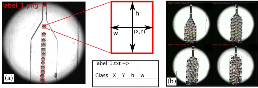
Figure 25: (a) A picture of a sequence of monodisperse droplets in a divergent microfluidic channel. This represents an example of a training dataset for YOLO. Each droplet is identified by a bounding box, whose dimensions are noted in an associated file. (b) Examples of DropTrack’s outputs, which identify and track droplets of a dense emulsion flowing in microchannels of different geometry. Copyright granted under the https://creativecommons.org/licenses/by/4.0/ CC 4.0 license. No changes were made to the original figures in Ref. Durve et al. (2023).

VI.3.1 Learning shape dynamics

In many soft matter applications, there is substantial scope for controlling not only the position and velocity of the single droplets, but also their shape changes as such droplets move along the flow. Since this adds a significant number of internal degrees of freedom, machine learning can find profitable use to accomplish this task as well. For instance, Li et al. Li et al. (2024) used machine learning techniques to predict the shape of bubble droplets to be used in a multiphase LB simulations using the pseudopotential method. A regularized feedforward deep neural network, made of a first hidden layer of fifty neurons and a second one of ten neurons, was then trained on this data with a gradient descent method, providing a R-coefficient ranging between 0.9965 and 1. However, the study is limited by the narrow range of surface tension (0.01 and 0.02) and viscosity ratios (0.05 and 0.10), as well as by the bi-dimensionality of the simulation. Recently, a class of machine learning methodologies, called autoencoder, has been employed to acquire minimal droplet shape descriptors, subsequently applied in forecasting droplet breakup occurrences Khor et al. (2019); Durve et al. (2024b), a process crucial in many industrial applications Rosenfeld et al. (2014b); Gai et al. (2016).

As a general goal, one may think of machine-learning as a useful tool to devise the effective equations of motion of suspended bodies, including internal degrees of freedom associated with the deformability of the soft bodies.

The corresponding set of effective dynamic equations for a set of $N_{d}$ droplets would take the following form.

1. For the external degrees of freedom, i.e. position $R_{i}$ and velocity $V_{i}$, the equations are:

$$\dot{R}_{i} = V_{i}$$ (95)

$$M_{i}\dot{V}_{i} = \sum_{j=1}^{N_{d}}f(R_{i},R_{j},u_{i},u_{j},a_{i},a_{j})\equiv\sum_{j=1}^{N_{d}}f_{ij},$$ (96)

where $u_{i}$ is the flow velocity at location $R_{i}$, and $a_{i}$ is the sequence of Fourier coefficients (a vector) describing the shape of the $i$-th droplet.

2. For the internal degrees of freedom, i.e. shape coefficients $a_{i}$, one has:

$$\dot{a}_{i}=\sum_{j=1}^{N_{d}}g(R_{i},R_{j},u_{i},u_{j},a_{i},a_{j})\equiv\sum_{j=1}^{N_{d}}g_{ij}$$ (97)

3. Finally, for the flow fields, the equations are:

$$\dot{u}_{i}=\sum_{j=1}^{N_{d}}h(R_{i},R_{j},u_{i},u_{j},a_{i},a_{j})\equiv\sum_{j=1}^{N_{d}}h_{ij}.$$ (98)

The above is a formidable problem since it involves functions of several thousands of variables: thousand droplets with, say, ten internal shape parameters each, generate $(6+10)\times 1000=16000$ dimensions. However, this is precisely the ground where machine learning may be expected to offer insights outside the reach of analytics and also large-scale numerics.

Incidentally, we do not expect reciprocity, that is $f_{ij}\neq f_{ji}$, $g_{ij}\neq g_{ji}$ and $h_{ij}\neq h_{ji}$ since the flow field, as well as the deformations, break both translational and rotational invariance. This is reminiscent of active-matter behavior and can indeed be related to self-propelling effects, along the lines pioneered by Shapere and Wilczek, where the problem of self-propulsion at low Reynolds number is formulated in terms of a gauge field over the space of shapes Shapere and Wilczek (1987); Wilczek (2022). In this respect, machine learning could be useful to inform a statistical theory of shape dynamics, with potential applications outside the realm of soft matter.

VI.4 Prospects for quantum computing of soft fluids

We finally discuss a further perspective about potential links between lattice Boltzmann and quantum computing. Indeed, quantum computing is one of the most vibrant topics of modern science, holding promises of spectacular applications far beyond the reach of classical electronic computers, if only for a limited set of applications Arute et al. (2019); Ippoliti et al. (2021). The main point is that qubits, the quantum analog of classical bits, represent an arbitrary superposition of the two fundamental states $|0>$ (ground state) and $|1>$ (excited state), so that a collection of $Q$ qubits spans an exponentially large Hilbert space, consisting of $2^{Q}$ classical states. The blue-sky scenario for fluids is mind-boggling. Given that a fluid flow at Reynolds number $Re$ consists of about $Re^{3}$ active degrees of freedom, the number of qubits required to represent such state-space is given by

$$Q(Re)=3Log_{2}Re\sim 10Log_{10}Re.$$ (99)

This expression shows that a flow at $Re=10^{8}$, basically the state-of-the-art of current electronic supercomputers, can be represented by mere $80$ qubits, which is well within the nominal capabilities of current quantum hardware Castelvecchi (2023), now offering several hundred physical qubits.

However, realizing this exponential advantage faces a number of steep technological and conceptual challenges. First, qubits decohere quite fast, in a matter of microseconds even with the best current-day quantum technology. Second, even when qubits are in a coherent superposition, quantum updates can still fail due to quantum noise, with a typical error rate around $10^{-3}$, to be contrasted with a classical error rate around $10^{-18}$! The end result, to date, is that the number of effective qubits that can be actually used to perform reliable simulations is at least a factor ten below the nominal value. Hence, a more realistic estimate is

$$Q(Re)\sim 100Log_{10}Re,$$ (100)

which means that reaching the exascale performance will require of the order of thousands effective qubits.

Realizing such potential for fluids meets with two additional challenges: nonlinearity and dissipation. Indeed, while quantum mechanics is linear and conservative, the physics of fluids is typically neither, hence additional procedures have to be devised to formulate quantum computing algorithms for fluids. Dissipation can be dealt with in several ways, for instance by adding a reservoir to the original quantum states, such as the union of the two conserves energy Mezzacapo et al. (2015). However, the non-unitary update of the system implies a non-zero probability of failure which accumulates in time, leading to a deterioration of efficiency.

Nonlinearity is a more fundamental problem. Several strategies are available to deal with it (for a recent review see Succi et al. (2023)), but in the following we shall briefly focus on one which has received particular attention in the last few years, namely Carleman linearization Carleman (1932).

The idea is very simple and best illustrated by means of a zero-dimensional nonlinear system, namely the logistic equation:

$$\frac{dx}{dt}=x(1-Rx),\;\;\;x(t=0)=x_{0}$$ (101)

where $R$ measures the strength of the nonlinearity. The Carleman procedure consists in renaming $x\equiv x_{1}$ and $x^{2}\equiv x_{2}$, so that the logistic equation takes the following form:

$$\frac{dx_{1}}{dt}=x_{1}-Rx_{2},$$ (102)

This is formally linear, but open, hence it requires an additional equation for $x_{2}$. This is easily derived by differentiating $x^{2}$, which yields

$$\frac{dx_{2}}{dt}=2(x_{2}-Rx_{3}),$$ (103)

which is again linear but in need of a closure for $x_{3}\equiv x^{3}$. Reiterating the procedure up to a generic level $k$, we obtain

$$\frac{dx_{k}}{dt}=k(x_{k}-Rx_{k+1})$$ (104)

which can be closed by setting $x_{k+1}=f(x_{k})$, the typical case being truncation $x_{k+1}=0$. The idea is clear, one trades nonlinearity in finite dimensions (just one variable in the logistic case) for a linear problem in infinite dimensions, in the hope that a low-order truncation can nevertheless provide an accurate approximation to the original problem. For the case of quantum computing for fluids, the point is to turn the nonlinear equations of fluids into a linear set of the form

$$\frac{dV}{dt}=CV$$ (105)

where $V$ is the set of fluid variables and $C$ is the associated Carleman matrix. Such a linear system could then in principle be solved by QLAS, Quantum Linear Algorithm Solver Harrow et al. (2009). The reality tells however a much more complicated story. First, the number of Carleman variables grows exponentially with the level of the Carleman truncation. For instance at level $k=1$ the relevant Carleman set of variables is $\{\rho,J_{a},J_{a}J_{b}/\rho\}$ , namely $1+3+6=10$ in dimension $d=3$. On a $1000^{3}$ grid, this makes $10^{10}$ variables, requiring $Q=100Log_{2}10\sim 330$ effective qubits. At the next Carleman level, we have all possible cross-couplings of the former terms which arise as one constructs the dynamic equation for $K_{ab}\equiv J_{a}J_{b}/\rho$, including coupling to the non-local dissipative term $\partial_{a}J_{b}$. This leads to $O(100)$ Carleman variables, hence $Q\sim 370$ qubits, which looks fine. However, this hinges on two additional assumptions: First, all couplings remain local; second, that the Carleman procedure shows satisfactory convergence already at Carleman level 2. By a suitable choice of the discrete scheme, the first requirement can be met. However, based on actual evidence, no satisfactory convergence is observed at moderate Reynolds numbers, $Re\sim O(10)$, over a significant period of time Sanavio and Succi (2023). To date, the only partially successful application is the simulation of a one-dimensional Burgers flow, with $16$ grid points over a few thousands time-steps Liu et al. (2021), truncated at the fourth Carleman level (see Fig.26).

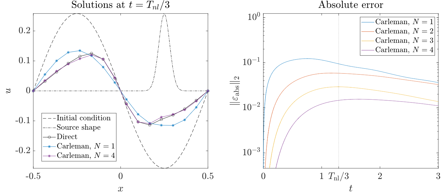
Figure 26: Left panel: Initial conditions, source and solutions of the velocity field of the Burger equation computed at Re=20 with a spatial discretization of 16 grid points and run on a classical computer. Right panel: $l_{2}$ norm of the absolute error between different Carleman truncation levels. Note that, the error of the Carleman method converges exponentially with $N$. Copyright (2021) National Academy of Sciences Ref.Liu et al. (2021).

Note however that the Carleman procedure applied to the Burgers equations is far simpler than Carleman applied to the Navier-Stokes equations.

It should be mentioned that much better convergence can be obtained by applying the Carleman procedure to the Lattice Boltzmann equation Itani and Succi (2022); Succi et al. (2023); Sanavio and Succi (2023). Unfortunately, the corresponding Carleman-LB algorithm is non-local, which reflects into an unviable depth of the corresponding quantum circuit. As a result, with the current state of affairs, the implementation of a quantum algorithm for fluid flows is still open. Coming back to soft flowing matter, the good news is that the Reynolds number is generally moderate, often below $100$, hence, once the aforementioned problems are solved (assuming they will), about a hundred effective qubits will suffice to quantum simulate complex states of soft flowing matter. Work along this line is currently in progress.

VII Conclusions

Summarizing we have discussed a series of Lattice Boltzmann methods to simulate microscale multi-component soft flows under strong geometric confinement. Such methods leverage the flexibility of the LB method to efficiently incorporate mesoscale physics beyond hydrodynamics and yet in no need of detailed molecular specificity. The inclusion of near-contact interactions via a simple repulsive force stands as a paradigmatic example of this approach and has proven successful for a broad variety of complex rheological applications which would be very hard to treat with different methods, particularly in the case of dense confined emulsions.

This success hinges on what we have called Extended Universality (EU), meaning by this the dependence on a series of dimensionless parameters rather than on the specifics of the near-contact interactions. In our case, near-contact interactions have been represented by a one-parameter repulsive force, but it is not hard to imagine situations where multi-parameter representations would be needed, if not a fully atomistic description. The quantum-nanofluidic applications discussed in the previous section is a likely candidate in this respect. Likewise, biological applications present many instances of broken EU, for instance it is known that cells develop major protrusions, called philopodes, whose task is to explore the surroundings and provide crucial feedback for the cell motion Bray (2000). Philopodes are nanometric structures whose shape and dynamics provides specific feedback to the cell, hence it is hard to imagine how they could be realistically modeled by a coarse-grained approach such as the one discussed in this review.

This indicates that there is much room for further refinement and enhancement of the techniques discussed in this work aimed towards a new generation of LB schemes with increasing molecular/chemical specificity.

For instance, most of this work relies on the direct simulation of about three decades in space, say millimeters to microns, leaving another two to three decades to a coarse-grained formulation of sub-micron interactions. In the future, the availability of exascale computers will allow for the direct simulation of four spatial decades, thereby reducing the range that needs to be covered by coarse-graining. Furthermore, the resort to machine learning can lead to more elaborated and specificity-aware coarse-grained models, such as those discussed in Section III.3, possibly combined with high-order-lattice implementations including statistical fluctuations and higher-order pre-hydrodynamic effects.

The concurrent progress of the three lines of development mentioned above is expected to take the next generation of specificity-aware LB models for soft flowing matter down to the ten nanometers scale, thus greatly facilitating the coupling to microscopic models.

Substantial work shall be needed to develop a robust and efficient specificity-aware LB models, but the prospects look decidedly bright and the range of applications extremely rich and challenging.

References

- Piazza (2012) R. Piazza, Soft Matter: The stuff that dreams are made of (Springer, Rotterdam Netherlands, 2012).
- Doi (2013) M. Doi, Soft Matter Physics (Oxford University Press, Oxford, 2013).
- Fernandez-Nieves and Puertas (2016) A. Fernandez-Nieves and A. M. Puertas, Fluids, Colloids and Soft Materials: An Introduction to Soft Matter Physics (John Wiley & Sons Inc, 2016).
- Kleman and Lavrentovich (2003) M. Kleman and O. Lavrentovich, Soft Matter Physics: An Introduction (Springer, 2003) p. 637.
- Nagel (2017) S. R. Nagel, “Experimental soft-matter science,” Rev. Mod. Phys. 89, 025002 (2017).
- Chen et al. (2010) D.T.N. Chen, Q. Wen, P. A. Janmey, J. C. Crocker, and A. G. Yodh, “Rheology of soft materials,” Annu. Rev. Cond. Matt. Phys. 1, 301–322 (2010).
- Hamley (2003) I. W. Hamley, “Nanotechnology with Soft Materials,” Angewandte Chemie International Edition 42, 1692–1712 (2003).
- Raven and Marmottant (2009) J. P. Raven and P. Marmottant, “Microfluidic crystals: Dynamic interplay between rearrangement waves and flow,” Phys. Rev. Lett. 102, 084501 (2009).
- Marmottant and Raven (2009) P. Marmottant and J. P. Raven, “Microfluidics with foams,” Soft matter 5, 3385–3388 (2009).
- Y. et al. (2016) Gai Y., C. M. Leong, W. Cai, and S. K. Y. Tang, “Spatiotemporal periodicity of dislocation dynamics in a two-dimensional microfluidic crystal flowing in a tapered channel,” Proceedings of the National Academy of Sciences 113, 12082–12087 (2016).
- Goyon and Bocquet (2010) A. Goyon, J. Colin and L. Bocquet, “How does a soft glassy material flow: finite size effects, non local rheology, and flow cooperativity,” Soft Matter 6, 2668 (2010).
- Utada et al. (2005) A. S. Utada, E. Lorenceau, D. R. Link, P. D. Kaplan, H. A. Stone, and D. A. Weitz, “Monodisperse double emulsions generated from a microcapillary device,” Science 308, 537–541 (2005).
- Datta et al. (2014) S.S. Datta, A. Abbaspourrad, E. Amstad, J. Fan, S.H. Kim, M. Romanowsky, H.C. Shum, B.J. Sun, A.S. Utada, M. Windbergs, S.B. Zhou, and D.A. Weitz, “25th anniversary article: Double emulsion templated solid microcapsules: Mechanics and controlled release,” Advanced Materials 26, 2205–2218 (2014).
- Kaminski et al. (2016) T. S. Kaminski, O. Scheler, and P. Garstecki, “Droplet microfluidics for microbiology: techniques, applications and challenges,” Lab Chip 16, 2168–2187 (2016).
- Bray (2000) D. Bray, Cell Movements: From Molecules to Motility (Routledge; 2nd. Edition, 2000) p. 386.
- Elacqua et al. (2018) J. J. Elacqua, A. L. McGregor, and J. Lammering, “Automated analysis of cell migration and nuclear envelope rupture in confined environments,” Plos One 13, e0195664 (2018).
- Davidson et al. (2015) P. M. Davidson, J. Sliz, P. Isermann, C. Denais, and J. Lammerding, “Design of a microfluidic device to quantify dynamic intra-nuclear deformation during cell migration through confining environments,” Integrative Biology 7, 1534–1546 (2015).
- Davidson et al. (2014) P. M. Davidson, C. Denais, M. C. Bakshi, and J. Lammerding, “Nuclear deformability constitutes a rate-limiting step during cell migration in 3-d environments,” Cel. Mol. Bioeng. 7, 293–306 (2014).
- Choi et al. (2016) C.-H. Choi, H. Wang, H. Lee, J.H. Kim, L. Zhang, A. Mao, D. J. Mooney, and D. A. Weitz, “One-step generation of cell-laden microgels using double emulsion drops with a sacrificial ultra-thin oil shell,” Lab Chip 16, 1549–1555 (2016).
- Mao et al. (2019) A. S. Mao, B. Özkale, N. J. Shah, K.H. Vining, T. Descombes, L. Zhang, C. M. Tringides, S. M. Wong, J. W. Shin, D. T. Scadden, D. A. Weitz, and D. J. Mooney, “Programmable microencapsulation for enhanced mesenchymal stem cell persistence and immunomodulation,” Proceedings of the National Academy of Sciences 116, 15392–15397 (2019).
- Adams et al. (2012) L. L. A. Adams, Thomas E. Kodger, Shin-Hyun Kim, Ho Cheng Shum, Thomas Franke, and David A. Weitz, “Single step emulsification for the generation of multi-component double emulsions,” Soft matter 8, 10719–10724 (2012).
- Bocquet and Charlaix (2010) L. Bocquet and E. Charlaix, “Nanofluidics, from bulk to interfaces,” Chem. Soc. Rev. 39, 1073–1095 (2010).
- Succi (2018) S. Succi, The lattice Boltzmann equation: for complex states of flowing matter (Oxford university press, 2018).
- Groot and Warren (1997) R. D. Groot and P. B. Warren, “Dissipative particle dynamics: Bridging the gap between atomistic and mesoscopic simulation,” The Journal of Chemical Physics 107, 4423–4435 (1997).
- Gompper et al. (2009) G. Gompper, T. Ihle, D. M. Kroll, and R. G. Winkler, “Multi-particle collision dynamics: A particle-based mesoscale simulation approach to the hydrodynamics of complex fluids,” in Advanced Computer Simulation Approaches for Soft Matter Sciences III, edited by Christian Holm and Kurt Kremer (Springer Berlin Heidelberg, Berlin, Heidelberg, 2009) pp. 1–87.
- Montessori et al. (2019a) A. Montessori, M. Lauricella, N. Tirelli, and S. Succi, “Mesoscale modelling of near-contact interactions for complex flowing interfaces,” Journal of Fluid Mechanics 872, 327–347 (2019a).
- Derjaguin and Landau (1941) B. Derjaguin and L. Landau, “A theory of the stability of strongly charged lyophobic sols and of the adhesion of strongly charged particles in solutions of electrolytes,” Acta Physico Chimica URSS 14, 633 (1941).
- Verwey and Overbeek (1948) E. J. W. Verwey and J. Th. G. Overbeek, “Theory of the stability of lyophobic colloids,” The Journal of Physical and Colloid Chemistry 51, 631–636 (1948).
- Lamoreaux (2004) S. K. Lamoreaux, “The Casimir force: background, experiments, and applications,” Rep. Prog. Phys. 68, 201 (2004).
- Krüger et al. (2017) T. Krüger, H. Kusumaatmaja, A. Kuzmin, O. Shardt, G. Silva, and E. M. Viggen, The Lattice Boltzmann Method: Principles and Practice (Springer International Publishing, 2017).
- Sukop and Thorne (2006) M. Sukop and D. Thorne, Lattice Boltzmann Modeling for geoscientists and engineers (Springer, 2006).
- Huang (2008) K. Huang, Statistical Mechanics (Wiley, 2008).
- Pathria and Beale (2011) R. K. Pathria and P. D. Beale, Statistical Mechanics (Elsevier, 2011).
- Kohn (1999) W. Kohn, “Nobel lecture: Electronic structure of matter-wave functions and density functionals,” Rev. Mod. Phys. 71, 1253 (1999).
- Hohenberg and Kohn (1964) P. Hohenberg and W. Kohn, “Inhomogeneous electron gas,” Phys. Rev. 136, B864 (1964).
- Kohn and Sham (1965) W. Kohn and L. J. Sham, “Self-consistent equations including exchange and correlation effects,” Phys. Rev. 140, A1133 (1965).
- Mourik et al. (2014) T. V. Mourik, M. Bühl, and M. P. Gaigeot, “Density functional theory across chemistry, physics and biology,” Phil. Trans. Roy. Soc. A 372, 20120488 (2014).
- Landau and Lifshitz (1987) L. D. Landau and E. M. Lifshitz, Fluid Mechanics: Volume 6 (Butterworth-Heinemann; 2nd edition, 1987).
- Bhatnagar et al. (1954) P. L. Bhatnagar, E. P. Gross, and M. Krook, “A model for collision processes in gases. i. Small amplitude processes in charged and neutral one-component systems,” Phys. Rev. 94, 511 (1954).
- Chapman and Cowling (1990) S. Chapman and T. G. Cowling, The mathematical theory of non-uniform gases: an account of the kinetic theory of viscosity, thermal conduction and diffusion in gases (Cambridge university press, 1990).
- Pitaevskii and Lifshitz (1981) L. P. Pitaevskii and E. M. Lifshitz, Physical Kinetics: Volume 10 (Butterworth-Heinemann; 1st edition, 1981).
- Riboff (2003) R. L. Riboff, Kinetic Theory: Classical, Quantum, and Relativistic Descriptions: Third Edition (Springer, 2003).
- Lallemand and Luo (2000) P. Lallemand and L.-S. Luo, “Theory of the lattice Boltzmann method: Dispersion, dissipation, isotropy, Galilean invariance, and stability,” Phys. Rev. E 61, 6546 (2000).
- d’Humières (2002) D. d’Humières, “Multiple–relaxation–time lattice Boltzmann models in three dimensions,” Phil. Trans. Roy. Soc. London. Ser. A: Math., Phys. and Eng. Sci. 360, 437–451 (2002).
- Fei et al. (2018a) L. Fei, K. H. Luo, C. Lin, and Q. Li, “Modeling incompressible thermal flows using a central-moments-based lattice Boltzmann method,” International Journal of Heat and Mass Transfer 120, 624–634 (2018a).
- Fei et al. (2018b) L. Fei, K. H. Luo, and Q. Li, “Three-dimensional cascaded lattice Boltzmann method: Improved implementation and consistent forcing scheme,” Phys. Rev. E 97, 053309 (2018b).
- Carenza et al. (2019) L. N. Carenza, G. Gonnella, A. Lamura, G. Negro, and A. Tiribocchi, “Lattice Boltzmann methods and active fluids,” Eur. Phys. Journ. E 42, 81 (2019).
- Gunstensen et al. (1991) A. K. Gunstensen, D. H. Rothman, S. Zaleski, and G. Zanetti, “Lattice Boltzmann model of immiscible fluids,” Phys. Rev. A 43, 4320–4327 (1991).
- Leclaire et al. (2012) S. Leclaire, M. Reggio, and J. Y. Trépanier, “Numerical evaluation of two recoloring operators for an immiscible two-phase flow lattice Boltzmann model,” Appl. Math. Model. 36, 2237–2252 (2012).
- Leclaire et al. (2017) S. Leclaire, A. Parmigiani, O. Malaspinas, B. Chopard, and J. Latt, “Generalized three-dimensional lattice Boltzmann color-gradient method for immiscible two-phase pore-scale imbibition and drainage in porous media,” Phys. Rev. E 95, 033306 (2017).
- Latva-Kokko and Rothman (2005) M. Latva-Kokko and D. H. Rothman, “Diffusion properties of gradient-based lattice Boltzmann models of immiscible fluids,” Phys. Rev. E 71, 056702 (2005).
- Brackbill et al. (1992) J. U. Brackbill, D. B. Kothe, and C. Zemach, “A continuum method for modeling surface tension,” Jour. Comput. Phys. 100, 335–354 (1992).
- Liu et al. (2012) H. Liu, A. J. Valocchi, and Q. Kang, “Three-dimensional lattice Boltzmann model for immiscible two-phase flow simulations,” Phys. Rev. E 85, 046309 (2012).
- Montessori et al. (2018a) A. Montessori, M. Lauricella, M. La Rocca, S. Succi, E. Stolovicki, R. Ziblat, and D. Weitz, “Regularized lattice Boltzmann multicomponent models for low capillary and reynolds microfluidics flows,” Comput. & Fluids 167, 33–39 (2018a).
- Montessori et al. (2015) A. Montessori, P. Prestininzi, M. La Rocca, and S. Succi, “Lattice Boltzmann approach for complex nonequilibrium flows,” Phys. Rev. E 92, 043308 (2015).
- Zhang et al. (2006) R. Zhang, X. Shan, and H. Chen, “Efficient kinetic method for fluid simulation beyond the Navier-Stokes equation,” Phys. Rev. E 74, 046703 (2006).
- Latt and Chopard (2006) J. Latt and B. Chopard, “Lattice Boltzmann method with regularized pre-collision distribution functions,” Mathematics and Computers in Simulation 72, 165–168 (2006).
- Coreixas et al. (2017) C. Coreixas, G. Wissocq, G. Puigt, J.-F. Boussuge, and P. Sagaut, “Recursive regularization step for high-order lattice Boltzmann methods,” Phys. Rev. E 96, 033306 (2017).
- Mattila et al. (2017) K. K. Mattila, P. C. Philippi, and L. A. Jr. Hegele, “High-order regularization in lattice Boltzmann equations,” Phys. Fluids 29, 046103 (2017).
- Hegele et al. (2018) L. A. Hegele, A. Scagliarini, M. Sbragaglia, K. K. Mattila, P. C. Philippi, D. F. Puleri, J. Gounley, and A. Randles, “High-Reynolds-number turbulent cavity flow using the lattice Boltzmann method,” Phys. Rev. E 98, 043302 (2018).
- Montessori et al. (2016) A. Montessori, P. Prestininzi, M. La Rocca, G. Falcucci, S. Succi, and E. Kaxiras, “Effects of Knudsen diffusivity on the effective reactivity of nanoporous catalyst media,” Jour. Comput. Sci. 17, 377–383 (2016).
- Succi et al. (1995) S. Succi, G. Amati, and R. Benzi, “Challenges in lattice Boltzmann computing,” J. Stat. Phys. 81, 5–16 (1995).
- Benzi et al. (1992) R. Benzi, S. Succi, and M. Vergassola, “The lattice Boltzmann equation: theory and applications,” Phys. Rep. 222, 145–197 (1992).
- Montessori et al. (2018b) A. Montessori, M. Lauricella, S. Succi, E. Stolovicki, and D. Weitz, “Elucidating the mechanism of step emulsification,” Phys. Rev. Fluids 3, 072202 (2018b).
- Chan et al. (2011) D. Y. C. Chan, E. Klaseboer, and R. Manica, “Film drainage and coalescence between deformable drops and bubbles,” Soft Matter 7, 2235–2264 (2011).
- Williams and Davis (1992) M. B. Williams and S. H. Davis, “Nonlinear theory of film rupture,” J. Colloid Interface Sci. 90, 220–228 (1992).
- Gupta et al. (2017) A. Gupta, A. Z. M Badruddoza, and P. S. Doyle, “A general route for nanoemulsion synthesis using low-energy methods at constant temperature,” Langmuir 33, 7118–7123 (2017).
- Nekovee et al. (2000) M. Nekovee, P. V. Coveney, H. Chen, and B. M. Boghosian, “Lattice-Boltzmann model for interacting amphiphilic fluids,” Phys. Rev. E 62, 8282–8294 (2000).
- Love et al. (2001) P. J. Love, P. V. Coveney, and B. M. Boghosian, “Three-dimensional hydrodynamic lattice-gas simulations of domain growth and self-assembly in binary immiscible and ternary amphiphilic fluids,” Phys. Rev. E 64, 021503 (2001).
- Chen et al. (2000) H. Chen, B. M. Boghosian, and P. V. Coveney, “A ternary lattice Boltzmann model for amphiphilic fluids,” Proc. Roy. Soc. Ser. A 456, 2043–2057 (2000).
- Swift et al. (1996) M. R. Swift, E. Orlandini, W. R. Osborn, and J. M. Yeomans, “Lattice Boltzmann simulations of liquid-gas and binary fluid systems,” Phys. Rev. E 54, 5041–5052 (1996).
- Swift et al. (1995) M. R. Swift, W. R. Osborn, and J. M. Yeomans, “Lattice Boltzmann simulation of nonideal fluids,” Phys. Rev. Lett. 75, 830–833 (1995).
- Shan and Chen (1993) X. Shan and H. Chen, “Lattice Boltzmann model for simulating flows with multiple phases and components,” Phys. Rev. E 47, 1815–1819 (1993).
- Shan and Doolen (1995) X. Shan and G. Doolen, “Multicomponent lattice-Boltzmann model with interparticle interaction,” J. Stat. Phys. 81, 379–393 (1995).
- Cahn and Hilliard (1958) J. W. Cahn and J. E. Hilliard, “Free energy of a nonuniform system. I. Interfacial free energy,” J. Chem. Phys. 28, 258–267 (1958).
- Foglino et al. (2017) M. Foglino, A. N. Morozov, O. Henrich, and D. Marenduzzo, “Flow of deformable droplets: Discontinuous shear thinning and velocity oscillations,” Phys. Rev. Lett. 119, 208002 (2017).
- Marchetti et al. (2013) M. C. Marchetti, J. F. Joanny, S. Ramaswamy, T. B. Liverpool, J. Prost, Madan Rao, and R. Aditi Simha, “Hydrodynamics of soft active matter,” Rev. Mod. Phys. 85, 1143–1189 (2013).
- Cates et al. (2009) M. E. Cates, O. Henrich, D. Marenduzzo, and K. Stratford, “Lattice Boltzmann simulations of liquid crystalline fluids: active gels and blue phases,” Soft Matter 5, 3791–3800 (2009).
- de Gennes and Prost (1993) P. G. de Gennes and J. Prost, The physics of liquid crystals (Oxford University Press, 2nd ed., 1993).
- Hatwalne et al. (2004) Y. Hatwalne, S. Ramaswamy, M. Rao, and R. A. Simha, “Rheology of active-particle suspensions,” Phys. Rev. Lett. 92, 118101 (2004).
- Pedley and Kessler (1992) T. J. Pedley and J. O. Kessler, “Hydrodynamic phenomena in suspensions of swimming microorganisms,” Ann. Rev. Fluid Mech. 24, 313 (1992).
- Gonnella et al. (2007) G. Gonnella, A. Lamura, and V. Sofonea, “Lattice Boltzmann simulation of thermal nonideal fluids,” Phys. Rev. E 76, 036703 (2007).
- Lamura et al. (1999) A. Lamura, G. Gonnella, and J. M. Yeomans, “A lattice Boltzmann model of ternary fluid mixtures,” Europhysics Letters 45, 314 (1999).
- Xu et al. (2003) A. Xu, G. Gonnella, and A. Lamura, “Phase-separating binary fluids under oscillatory shear,” Phys. Rev. E 67, 056105 (2003).
- Xu et al. (2006) A. Xu, G. Gonnella, and A. Lamura, “Morphologies and flow patterns in quenching of lamellar systems with shear,” Phys. Rev. E 74, 011505 (2006).
- Gonnella et al. (2010) G. Gonnella, A. Lamura, A. Piscitelli, and A. Tiribocchi, “Phase separation of binary fluids with dynamic temperature,” Phys. Rev. E 82, 046302 (2010).
- Tiribocchi et al. (2011a) A. Tiribocchi, A. Piscitelli, G. Gonnella, and A. Lamura, “Pattern study of thermal phase separation for binary fluid mixtures,” Int. J. Num. Meth. Heat & Fluid Flow 21, 572–583 (2011a).
- Tiribocchi et al. (2021a) A. Tiribocchi, A. Montessori, M. Durve, F. Bonaccorso, M. Lauricella, and S. Succi, “Dynamics of polydisperse multiple emulsions in microfluidic channels,” Phys. Rev. E 104, 065112 (2021a).
- Tiribocchi et al. (2020a) A. Tiribocchi, A. Montessori, S. Aime, M. Milani, M. Lauricella, S. Succi, and D. Weitz, “Novel nonequilibrium steady states in multiple emulsions,” Physics of Fluids 32, 017102 (2020a).
- Tiribocchi et al. (2021b) A. Tiribocchi, A. Montessori, F. Bonaccorso, M. Lauricella, and S. Succi, “Shear dynamics of polydisperse double emulsions,” Physics of Fluids 33, 047105 (2021b).
- Tiribocchi et al. (2021c) A. Tiribocchi, A. Montessori, M. Lauricella, F. Bonaccorso, S. Succi, S. Aime, M. Miliani, and D. A. Weitz, “The vortex-driven dynamics of droplets within droplets,” Nature Commun. 12, 82 (2021c).
- Stratford et al. (2014) K. Stratford, O. Henrich, J. Lintuvuori, M. E. Cates, and D. Marenduzzo, “Self-assembly of colloid-cholesteric composites provides a possible route to switchable optical materials,” Nature Commun. 5, 3954 (2014).
- Lesniewska et al. (2024) M. Lesniewska, N. Mottram, and O. Henrich, “Defect-influenced particle advection in highly confined liquid crystal flows,” Soft matter 20, 2218–2231 (2024).
- Denniston et al. (2004) C. Denniston, D. Marenduzzo, E. Orlandini, and J. M. Yeomans, “Lattice Boltzmann algorithm for three-dimensional liquid-crystal hydrodynamics,” Phil. Trans. Roy. Soc. A 362, 1745–1754 (2004).
- Sulaiman et al. (2006) N. Sulaiman, D. Marenduzzo, and J. M. Yeomans, “Lattice boltzmann algorithm to simulate isotropic-nematic emulsions,” Phys. Rev. E 74, 041708 (2006).
- Marenduzzo et al. (2004) D. Marenduzzo, E. Orlandini, and J. M. Yeomans, “Permeative flows in cholesteric liquid crystals,” Phys. Rev. Lett. 92, 188301 (2004).
- Marenduzzo et al. (2008) D. Marenduzzo, E. Orlandini, M.E. Cates, and J.M. Yeomans, “Lattice Boltzmann simulations of spontaneous flow in active liquid crystals: The role of boundary conditions,” Journal of Non-Newtonian Fluid Mechanics 149, 56–62 (2008).
- Tiribocchi et al. (2011b) A. Tiribocchi, G. Gonnella, D. Marenduzzo, E. Orlandini, and F. Salvadore, “Bistable defect structures in blue phase devices,” Phys. Rev. Lett. 107, 237803 (2011b).
- Tiribocchi et al. (2010) A. Tiribocchi, G. Gonnella, D. Marenduzzo, and E. Orlandini, “Switching and defect dynamics in multistable liquid crystal devices,” Applied Physics Letters 97, 143505 (2010).
- Tiribocchi et al. (2014) A. Tiribocchi, O. Henrich, J. S. Lintuvuori, and D. Marenduzzo, “Switching hydrodynamics in liquid crystal devices: a simulation perspective,” Soft matter 10, 4580–4592 (2014).
- Tiribocchi et al. (2013) A. Tiribocchi, M. E. Cates, G. Gonnella, D. Marenduzzo, and E. Orlandini, “Flexoelectric switching in cholesteric blue phases,” Soft matter 9, 4831–4842 (2013).
- Marenduzzo et al. (2007a) D. Marenduzzo, E. Orlandini, M. E. Cates, and J. M. Yeomans, “Steady-state hydrodynamic instabilities of active liquid crystals: Hybrid lattice Boltzmann simulations,” Phys. Rev. E 76, 031921 (2007a).
- Cates et al. (2008) M. E. Cates, S. M. Fielding, D. Marenduzzo, E. Orlandini, and J. M. Yeomans, “Shearing active gels close to the isotropic-nematic transition,” Phys. Rev. Lett. 101, 068102 (2008).
- Shendruk et al. (2017) T. N. Shendruk, A. Doostmohammadi, K. Thijssen, and J. M. Yeomans, “Dancing disclinations in confined active nematics,” Soft matter 13, 3853–3862 (2017).
- Marenduzzo et al. (2007b) D. Marenduzzo, E. Orlandini, and J. M. Yeomans, “Hydrodynamics and rheology of active liquid crystals: A numerical investigation,” Phys. Rev. Lett. 98, 118102 (2007b).
- De Magistris et al. (2014) G. De Magistris, A. Tiribocchi, C. A. Whitfield, R. J. Hawkins, M. E. Cates, and D. Marenduzzo, “Spontaneous motility of passive emulsion droplets in polar active gels,” Soft Matter 10, 7826–7837 (2014).
- Negro et al. (2019) G. Negro, L. N. Carenza, A. Lamura, A. Tiribocchi, and G. Gonnella, “Rheology of active polar emulsions: from linear to unidirectional and inviscid flow, and intermittent viscosity,” Soft matter 15, 8251–8265 (2019).
- Bonelli et al. (2016) F. Bonelli, G. Gonnella, A. Tiribocchi, and D. Marenduzzo, “Spontaneous flow in polar active fluids: the effect of a phenomenological self propulsion-like term,” Eur. Phys. J. E 39, 1 (2016).
- Bonelli et al. (2019) F. Bonelli, L. N. Carenza, G. Gonnella, D. Marenduzzo, E. Orlandini, and A. Tiribocchi, “Lamellar ordering, droplet formation and phase inversion in exotic active emulsions,” Sci. Rep. 9, 2801 (2019).
- Tiribocchi et al. (2023a) A. Tiribocchi, M. Durve, M. Lauricella, A. Montessori, D. Marenduzzo, and S. Succi, “Shapes and dynamic regimes of a polar active fluid droplet under confinement,” Physics of Fluids 35, 063106 (2023a).
- Tiribocchi et al. (2023b) A. Tiribocchi, M. Durve, M. Lauricella, A. Montessori, and S. Succi, “Spontaneous motion of a passive fluid droplet in an active microchannel,” Soft matter 19, 6556–6568 (2023b).
- Tiribocchi et al. (2009) A. Tiribocchi, N. Stella, G. Gonnella, and A. Lamura, “Hybrid lattice Boltzmann model for binary fluid mixtures,” Phys. Rev. E 80, 026701 (2009).
- Thampi et al. (2013) S. P. Thampi, S. Ansumali, R. Adhikari, and S. Succi, “Isotropic discrete laplacian operators from lattice hydrodynamics,” Journal of Computational Physics 234, 1–7 (2013).
- Henrich et al. (2010) O. Henrich, D. Marenduzzo, K. Stratford, and M. E. Cates, “Domain growth in cholesteric blue phases: Hybrid lattice Boltzmann simulations,” Computers & Mathematics with Applications 59, 2360–2369 (2010).
- Hosseini et al. (2023) S. A. Hosseini, M. Atif, S. Ansumali, and I. V. Karlin, “Entropic lattice Boltzmann methods: A review,” Computers & Fluids 259, 105884 (2023).
- Montessori et al. (2017) A. Montessori, P. Prestininzi, M. La Rocca, and S. Succi, “Entropic lattice pseudo-potentials for multiphase flow simulations at high Weber and Reynolds numbers,” Phys. Fluids 29, 092103 (2017).
- Zou and He (1997) Q. Zou and X. He, “On pressure and velocity boundary conditions for the lattice Boltzmann BGK model,” Phys. Fluids 9, 1591 (1997).
- Lamura and Gonnella (2001) A. Lamura and G. Gonnella, “Lattice Boltzmann simulations of segregating binary fluid mixtures in shear flow,” Physica A 294, 295–312 (2001).
- Succi et al. (2019) S. Succi, G. Amati, M. Bernaschi, G. Falcucci, M. Lauricella, and A. Montessori, “Towards exascale lattice Boltzmann computing,” Computers & Fluids 181, 107–115 (2019).
- Shet et al. (2013) A. G. Shet, K. Siddharth, Shahajhan H. Sorathiya, A. M. Deshpande, S. D. Sherlekar, B. Kaul, and S. Ansumali, “On vectorization for lattice based simulations,” Int. Journ. Mod. Phys. C 24, 1340011 (2013).
- Namburi et al. (2016) M. Namburi, S. Krithivasan, and S. Ansumali, “Crystallographic lattice Boltzmann method,” Sci. Rep. 6, 27172 (2016).
- Bailey et al. (2009) P. Bailey, J. Myre, S. D. C. Walsh, D. J. Lilja, and M. O. Saar, “Accelerating lattice Boltzmann fluid flow simulations using graphics processors,” in 2009 international conference on parallel processing (IEEE, 2009) pp. 550–557.
- Lehmann (2022) M. Lehmann, “Esoteric pull and esoteric push: Two simple in-place streaming schemes for the lattice Boltzmann method on gpus,” Computation 10, 92 (2022).
- Geier and Schönherr (2017) M. Geier and M. Schönherr, “Esoteric twist: An efficient in-place streaming algorithmus for the lattice Boltzmann method on massively parallel hardware,” Computation 5, 19 (2017).
- Lehmann et al. (2022) M. Lehmann, M. J. Krause, G. Amati, M. Sega, J. Harting, and S. Gekle, “Accuracy and performance of the lattice Boltzmann method with 64-bit, 32-bit, and customized 16-bit number formats,” Phys. Rev. E 106, 015308 (2022).
- Gray and Boek (2016) F. Gray and E. Boek, “Enhancing computational precision for lattice Boltzmann schemes in porous media flows,” Computation 4, 11 (2016).
- Skordos (1993) P. A. Skordos, “Initial and boundary conditions for the lattice Boltzmann method,” Phys. Rev. E 48, 4823 (1993).
- Ladd and Verberg (2001) A.J.C. Ladd and R. Verberg, “Lattice-Boltzmann simulations of particle-fluid suspensions,” J. Stat. Phys. 104, 1191–1251 (2001).
- Tiribocchi et al. (2023c) A. Tiribocchi, A. Montessori, G. Amati, M. Bernaschi, F. Bonaccorso, S. Orlandini, S. Succi, and M. Lauricella, “Lightweight lattice Boltzmann,” J. Chem. Phys. 158 (2023c), 10.1063/5.0139850.
- Montessori et al. (2023) A. Montessori, M. Lauricella, A. Tiribocchi, M. Durve, M. La Rocca, G. Amati, F. Bonaccorso, and S. Succi, “Thread-safe lattice Boltzmann for high-performance computing on GPUs,” Journal of Computational Science 74, 102165 (2023).
- Montessori et al. (2024) A. Montessori, M. La Rocca, G. Amati, M. Lauricella, A. Tiribocchi, and S Succi, “High-order thread-safe lattice Boltzmann model for high performance computing turbulent flow simulations,” Phys. Fluids 36, 035171 (2024).
- Krüger et al. (2009) T. Krüger, F. Varnik, and D. Raabe, “Shear stress in lattice Boltzmann simulations,” Phys. Rev. E 79, 046704 (2009).
- Latt et al. (2008) J. Latt, B. Chopard, O. Malaspinas, M. Deville, and A. Michler, “Straight velocity boundaries in the lattice Boltzmann method,” Phys. Rev. E 77, 056703 (2008).
- Shan et al. (2006) X. Shan, X.-F. Yuan, and H. Chen, “Kinetic theory representation of hydrodynamics: a way beyond the Navier-Stokes equation,” Jour. Fluid Mech. 550, 413–441 (2006).
- Tucny et al. (2022) J.-M. Tucny, D. Vidal, S. Leclaire, and F. Bertrand, “Kinetic slip boundary condition for isothermal rarefied gas flows through static non-planar geometries based on the regularized lattice-boltzmann method,” Communications in Computational Physics 31, 816–868 (2022).
- Argentini et al. (2004) R. Argentini, A.F. Bakker, and C.P. Lowe, “Efficiently using memory in lattice Boltzmann simulations,” Future Generation Computer Systems 20, 973–980 (2004).
- Ferrari et al. (2023) M. A. Ferrari, W. B. de Oliveira Jr, A. Lugarini, A. T. Franco, and L. A. Hegele Jr, “A graphic processing unit implementation for the moment representation of the lattice Boltzmann method,” International Journal for Numerical Methods in Fluids (2023), 10.1002/fld.5185.
- Gounley et al. (2021) J. Gounley, M. Vardhan, E. W. Draeger, P. Valero-Lara, S. V. Moore, and A. Randles, “Propagation pattern for moment representation of the lattice Boltzmann method,” IEEE Transactions on Parallel and Distributed Systems 33, 642–653 (2021).
- Vardhan et al. (2019) M. Vardhan, J. Gounley, L. Hegele, E. W. Draeger, and A. Randles, “Moment representation in the lattice Boltzmann method on massively parallel hardware,” in Proceedings of the International Conference for High Performance Computing, Networking, Storage and Analysis (2019) pp. 1–21.
- Bader (2012) M. Bader, Space-filling curves: an introduction with applications in scientific computing, Vol. 9 (Springer Science & Business Media, 2012).
- Montessori et al. (2019b) A. Montessori, M. Lauricella, A. Tiribocchi, and S. Succi, “Modeling pattern formation in soft flowing crystals,” Phys. Rev. Fluids 4, 072201(R) (2019b).
- Montessori et al. (2020) A. Montessori, A. Tiribocchi, F. Bonaccorso, M. Lauricella, and S. Succi, “Lattice Boltzmann simulations capture the multiscale physics of soft flowing crystals,” Phil. Trans. Roy. Soc., Ser A. 378, 20190406 (2020).
- Garstecki et al. (2004) P. Garstecki, I. Gitlin, W. DiLuzio, G. M. Whitesides, E. Kumacheva, and H. A. Stone, “Formation of monodisperse bubbles in a microfluidic flow-focusing device,” Appl. Phys. Lett. 85, 2649–2651 (2004).
- Nan et al. (2024) L. Nan, H. Zhang, D. A. Weitz, and H. C. Shum, “Development and future of droplet microfluidics,” Lab Chip 24, 1135–1153 (2024).
- Xu et al. (2005) S. Xu, Z. Nie, M. Seo, P. Lewis, E. Kumacheva, H. A. Stone, P. Garstecki, D. B. Weibel, I. Gitlin, and G. M. Whitesides, “Generation of monodisperse particles by using microfluidics: Control over size, shape, and composition,” Angewandte Chemie 117, 734–738 (2005).
- Costantini et al. (2014) M. Costantini, C. Colosi, J. Guzowski, A. Barbetta, J. Jaroszewicz, S. Swieszkowski, M. Dentini, and P. Garstecki, “Highly ordered and tunable polyhipes by using microfluidics,” J. Mater. Chem. B 2, 2290–2300 (2014).
- Graner et al. (2008) F. Graner, B. Dollet, C. Raufaste, and P. Marmottant, “Discrete rearranging disordered patterns, part i: Robust statistical tools in two or three dimensions,” Eur. Phys. J. E 25, 349–369 (2008).
- Marmottant et al. (2008) P. Marmottant, C. Raufaste, and F. Graner, “Discrete rearranging disordered patterns, part ii: 2d plasticity, elasticity and flow of a foam,” Eur. Phys. J. E 25, 371–384 (2008).
- Weaire and Hutzler (2001) D. Weaire and S. Hutzler, The Physics of Foams (Oxford University Press, 2001).
- Gai et al. (2022) Y. Gai, A. Montessori, S. Succi, and S. K. Y. Tang, “Collective behavior of crowded drops in microfluidic systems,” Phys. Rev. Fluids 7, 080501 (2022).
- Luo et al. (2021) K. H. Luo, L. Fei, and G. Wang, “A unified lattice Boltzmann model and application to multiphase flows,” Phil. Trans. Roy. Soc. A 379, 2208 (2021).
- Montessori et al. (2021a) A. Montessori, M. La Rocca, P. Prestininzi, A. Tiribocchi, and S. Succi, “Deformation and breakup dynamics of droplets within a tapered channel,” Phys. Fluids 33, 082008 (2021a).
- Montessori et al. (2021b) A. Montessori, A. Tiribocchi, M. Lauricella, F. Bonaccorso, and S. Succi, “Wet to dry self-transitions in dense emulsions: From order to disorder and back,” Phys. Rev. Fluids 6 (2021b), 10.1103/PhysRevFluids.6.023606.
- Karnakov et al. (2022) P. Karnakov, S. Litvinov, and P. Koumoutsakos, “Computing foaming flows across scales: From breaking waves to microfluidics,” Sci. Adv. 8, 5 (2022).
- Montessori et al. (2021c) A. Montessori, A. Tiribocchi, M. Bogdan, F. Bonaccorso, M. Lauricella, J. Guzowski, and S. Succi, “Translocation dynamics of high-internal phase double emulsions in narrow channels,” Langmuir 37, 9026–9033 (2021c).
- Guzowski and Garstecki (2015) J. Guzowski and P. Garstecki, “Droplet clusters: Exploring the phase space of soft mesoscale atoms,” Phys. Rev. Lett. 114, 188302 (2015).
- Bogdan et al. (2022) M. Bogdan, A. Montessori, A. Tiribocchi, F. Bonaccorso, M. Lauricella, L. Jurkiewicz, S. Succi, and J. Guzowski, “Stochastic jetting and dripping in confined soft granular flows,” Phys. Rev. Lett. 128, 128001 (2022).
- Abate and Weitz (2009) A. R. Abate and D. A. Weitz, “High-order multiple emulsions formed in poly(dimethylsiloxane) microfluidics,” Small 5, 2030–2032 (2009).
- Cohen-Addad et al. (2013) S. Cohen-Addad, R. Höhler, and O. Pitois, “Flow in foams and flowing foams,” Annu. Rev. Fluid Mech. 45, 241 (2013).
- Douezan et al. (2011) S. Douezan, K. Guevorkian, R. Naouar, S. Dufour, D. Cuvelier, and F. Brochard-Wyart, “Spreading dynamics and wetting transition of cellular aggregates,” Proc. Natl. Acad. Sci. USA 108, 7315 (2011).
- Marmottant and Graner (2013) P. Marmottant and F. Graner, “Plastic and viscous dissipations in foams: Cross-over from low to high shear rates,” Soft Matter 9, 9602 (2013).
- Dollet et al. (2015) B. Dollet, A. Scagliarini, and M. Sbragaglia, “Two-dimensional plastic flow of foams and emulsions in a channel: experiments and lattice boltzmann simulations,” Journal of Fluid Mechanics 766, 556–589 (2015).
- Jiang et al. (1999) Yi Jiang, Pieter J. Swart, Avadh Saxena, Marius Asipauskas, and James A. Glazier, “Hysteresis and avalanches in two-dimensional foam rheology simulations,” Phys. Rev. E 59, 5819–5832 (1999).
- Wang et al. (2013) Jingtao Wang, Jinxia Liu, Junjie Han, and Jing Guan, “Effects of complex internal structures on rheology of multiple emulsions particles in 2d from a boundary integral method,” Phys. Rev. Lett. 110, 066001 (2013).
- Lulli et al. (2018) M. Lulli, R. Benzi, and M. Sbragaglia, “Metastability at the yield-stress transition in soft glasses,” Phys. Rev. X 8, 021031 (2018).
- Bonn et al. (2017) D. Bonn, M. M. Denn, L. Berthier, T. Divoux, and S. Manneville, “Yield stress materials in soft condensed matter,” Rev. Mod. Phys. 89, 035005 (2017).
- Sbragaglia et al. (2012) M. Sbragaglia, R. Benzi, M. Bernaschi, and S. Succi, “The emergence of supramolecular forces from lattice kinetic models of non-ideal fluids: applications to the rheology of soft glassy materials,” Soft Matter 8, 10773–10782 (2012).
- Rosenfeld et al. (2014a) L. Rosenfeld, L. Fan, J. Chen, R. Swoboda, and S. K. Y. Tang, “Break-up of droplets in a concentrated emulsion flowing through a narrow constriction,” Soft matter 10, 421–430 (2014a).
- Au et al. (2016) Sam H. Au, Brian D. Storey, John C. Moore, Qin Tang, Yeng-Long Chen, Sarah Javaid, A. Fatih Sarioglu, Ryan Sullivan, Marissa W. Madden, Ryan O’Keefe, Daniel A. Haber, Shyamala Maheswaran, David M. Langenau, Shannon L. Stott, and Mehmet Toner, “Clusters of circulating tumor cells traverse capillary-sized vessels,” Proceedings of the National Academy of Sciences 113, 4947–4952 (2016).
- Utada et al. (2007) A. S. Utada, A. Fernandez-Nieves, H. A. Stone, and D. A. Weitz, “Dripping to jetting transitions in coflowing liquid streams,” Phys. Rev. Lett. 99, 094502 (2007).
- Benzi et al. (2009) R. Benzi, M. Sbragaglia, S. Succi, M. Bernaschi, and S. Chibbaro, “Mesoscopic lattice boltzmann modeling of soft-glassy systems: Theory and simulations,” J. Chem. Phys. 131, 104903 (2009).
- Benzi et al. (2014) R. Benzi, M. Sbragaglia, P. Perlekar, M. Bernaschi, S. Succi, and F. Toschi, “Direct evidence of plastic events and dynamic heterogeneities in soft-glasses,” Soft Matter 10, 4615–4624 (2014).
- Pelusi et al. (2019) F. Pelusi, M. Sbragaglia, and R. Benzi, “Avalanche statistics during coarsening dynamics,” Soft Matter 15, 4518–4524 (2019).
- Tiribocchi et al. (2019) A. Tiribocchi, F. Bonaccorso, M. Lauricella, S. Melchionna, A. Montessori, and S. Succi, “Curvature dynamics and long-range effects on fluidfluid interfaces with colloids,” Soft Matter 15, 2848–2862 (2019).
- Voit et al. (2005) A. Voit, A. Krekov, W. Enge, L. Kramer, and W. Kölher, “Thermal patterning of a critical polymer blend,” Phys. Rev. Lett. 94, 2014501 (2005).
- Stein and Spera (1992) D. J. Stein and F. J. Spera, “Shear viscosity of rhyolite-vapor emulsions at magmatic temperatures by concentric cylinder rheometry,” J. Volcanol. Geoterm. Res. 49, 157–174 (1992).
- Pelusi et al. (2022) F. Pelusi, M. Lulli, M. Sbragaglia, and M. Bernaschi, “TLBfind: a thermal lattice Boltzmann code for concentrated emulsions with finite-size droplets,” Computer Physics Communications 273, 108259 (2022).
- Pelusi et al. (2021) F. Pelusi, M. Sbragaglia, R. Benzi, A. Scagliarini, M. Bernaschi, and S. Succi, “Rayleigh-Bénard convection of a model emulsion: anomalous heat-flux fluctuations and finite-size droplet effects,” Soft Matter 17, 3709–3721 (2021).
- Rayleigh (1916) R. Rayleigh, “On convection currents in a horizontal layer of fluid when the higher temperature is on the underside,” Philos. Mag. 32, 529–546 (1916).
- Bénard (1900) H. Bénard, “Les tourbillons cellulaires dans une nappe liquide.” Rev. Gen. Sci. Pures. Appl. 11, 1261–1271 (1900).
- Lohse and Xia (2010) D. Lohse and K. Q. Xia, “Small-scale properties of turbulent Rayleigh-Bénard convection,” Annu. Rev. Fluid Mech. 42, 335–364 (2010).
- Foglino et al. (2018) M. Foglino, A. N Morozov, and D. Marenduzzo, “Rheology and microrheology of deformable droplet suspensions,” Soft matter 14, 9361–9367 (2018).
- Negro et al. (2023) G. Negro, L. N. Carenza, G. Gonnella, F. Mackay, A. N. Morozov, and D. Marenduzzo, “Yield-stress transition in suspensions of deformable droplets,” Science Advances 9, 22 (2023).
- Loewe et al. (2020) B. Loewe, M. Chiang, D. Marenduzzo, and M. C. Marchetti, “Solid-liquid transition of deformable and overlapping active particles,” Phys. Rev. Lett. 125, 038003 (2020).
- Mueller et al. (2019) R. Mueller, J. M. Yeomans, and A. Doostmohammadi, “Emergence of active nematic behavior in monolayers of isotropic cells,” Phys. Rev. Lett. 122, 048004 (2019).
- Armengol-Collado et al. (2023) J.M. Armengol-Collado, L. N. Carenza, J. Eckert, D. Krommydas, and L. Giomi, “Epithelia are multiscale active liquid crystals,” Nature Physics 19, 1773–1779 (2023).
- Tiribocchi et al. (2020b) A. Tiribocchi, A. Montessori, F. Bonaccorso, M. Lauricella, and S. Succi, “Concentrated phase emulsion with multicore morphology under shear: A numerical study,” Phys. Rev. Fluids 5, 113606 (2020b).
- Wöhrwag et al. (2018) M. Wöhrwag, C. Semprebon, A. Mazloomi Moqaddam, I. Karlin, and H. Kusumaatmaja, “Ternary free-energy entropic lattice Boltzmann model with a high density ratio,” Phys. Rev. Lett. 120, 234501 (2018).
- Wang et al. (2020) N. Wang, C. Semprebon, H. Liu, C. Zhang, and H. Kusumaatmaja, “Modelling double emulsion formation in planar flow-focusing microchannels,” J. Fluid. Mech 895, A22 (2020).
- Abate et al. (2011) A. R. Abate, J. Thiele, and D. A. Weitz, “One-step formation of multiple emulsions in microfluidics,” Lab on a Chip 11, 253–258 (2011).
- Azarmanesh et al. (2016) M. Azarmanesh, M. Farhadi, and P. Azizian, “Double emulsion formation through hierarchical flow-focusing microchannel,” Physics of Fluids 28, 032005 (2016).
- Ramaswamy (2010) Sriram Ramaswamy, “The mechanics and statistics of active matter,” Annual Review of Condensed Matter Physics 1, 323–345 (2010).
- Sanchez et al. (2012) T. Sanchez, D.T.N. Chen, S.J. DeCamp, M. Heymann, and Z. Dogic, “Spontaneous motion in hierarchically assembled active matter,” Nature 491, 431–434 (2012).
- Michelin (2023) S. Michelin, “Self-propulsion of chemically active droplets,” Annu. Rev. Fluid Mech. 55, 77–101 (2023).
- Seemann et al. (2016) R. Seemann, JB. Fleury, and C.C. Maass, “Self-propelled droplets,” Eur. Phys. J. Spec. Top. 225, 2227–2240 (2016).
- Guillamat et al. (2018) P. Guillamat, Z. Kos, J. Hardoüin, J. Ignés-Mullol, M. Ravnik, and F. Sagués, “Active nematic emulsions,” Science Advances 4, eaao1470 (2018).
- Doostmohammadi et al. (2018) A. Doostmohammadi, J. Ignés Mullol, J. M. Yeomans, and F. Sagués, “Active nematics,” Nature Commun. 9, 3246 (2018).
- Ruske and Yeomans (2021) L. J. Ruske and J. M. Yeomans, “Morphology of active deformable 3d droplets,” Phys. Rev. X 11, 021001 (2021).
- Poincloux et al. (2011) R. Poincloux, O. Collin, F. Lizárraga, M. Romao, M. Debray, M. Piel, and P. Chavrier, “Contractility of the cell rear drives invasion of breast tumor cells in 3d matrigel,” Proceedings of the National Academy of Sciences 108, 1943–1948 (2011).
- Tjhung et al. (2012) E. Tjhung, D. Marenduzzo, and M. E. Cates, “Spontaneous symmetry breaking in active droplets provides a generic route to motility,” Proceedings of the National Academy of Sciences 109, 12381–12386 (2012).
- Tjhung et al. (2017) E. Tjhung, M. E. Cates, and D. Marenduzzo, “Contractile and chiral activities codetermine the helicity of swimming droplet trajectories,” Proceedings of the National Academy of Sciences 114, 4631–4636 (2017).
- Sakamoto et al. (2022) Ryota Sakamoto, Ziane Izri, Yuta Shimamoto, Makito Miyazaki, and Yusuke T. Maeda, “Geometric trade-off between contractile force and viscous drag determines the actomyosin-based motility of a cell-sized droplet,” Proceedings of the National Academy of Sciences 119, e2121147119 (2022).
- Ziebert and Aranson (2016) F. Ziebert and I. S. Aranson, “Computational approaches to substrate-based cell motility,” npj Computational Materials 2, 16019 (2016).
- Tjhung et al. (2015) E. Tjhung, A. Tiribocchi, D. Marenduzzo, and M. E. Cates, “A minimal physical model captures the shapes of crawling cells,” Nature Commun. 6, 5420 (2015).
- Giomi and DeSimone (2014) L. Giomi and A. DeSimone, “Spontaneous division and motility in active nematic droplets,” Phys. Rev. Lett. 112, 147802 (2014).
- Li et al. (2018) M. Li, M. Brinkmann, I. Pagonabarraga, R. Seemann, and J. B. Fleury, “Spatiotemporal control of cargo delivery performed by programmable self-propelled janus droplets,” Communication Physics 1, 23 (2018).
- Saw et al. (2017) T. B. Saw, A. Doostmohammadi, V. Nier, L. Kocgozlu, S. Thampi, Y. Toyama, P. Marcq, C. T. Lim, J. M. Yeomans, and B. Ladoux, “Topological defects in epithelia govern cell death and extrusion,” Nature 544, 212–216 (2017).
- Cao et al. (2016) X. Cao, E. Moeendarbary, P. Isermann, P. M. Davidson, X. Wang, M. B. Chen, A. K. Burkart, J. Lammerding, R. D. Kamm, and V. B. Shenoy, “A chemomechanical model for nuclear morphology and stresses during cell transendothelial migration,” Biophysical Journal 111, 1541–1552 (2016).
- Brückner et al. (2019) D. B. Brückner, A. Fink, C. Schreiber, P. J. Röttgermann, J. O. Rädler, and C. P. Broedersz, “Stochastic nonlinear dynamics of confined cell migration in two-state systems,” Nature Physics 15, 595–601 (2019).
- Tiribocchi et al. (2023d) A. Tiribocchi, M. Durve, M. Lauricella, A. Montessori, D. Marenduzzo, and S. Succi, “The crucial role of adhesion in the transmigration of active droplets through interstitial orifices,” Nature Commun. 14, 1096 (2023d).
- Falcucci et al. (2021) G. Falcucci, G. Amati, P. Fanelli, V. K. Krastev, G. Polverino, M. Porfiri, and S. Succi, “Extreme flow simulations reveal skeletal adaptations of deep-sea sponges,” Nature 595, 537–541 (2021).
- Monn et al. (2015) M. A. Monn, J. C. Weaver, T. Zhang, J. Aizenberg, and H. Kesari, “New functional insights into the internal architecture of the laminated anchor spicules of Euplectella aspergillum,” Proc. Natl. Acad. Sci. USA 112, 4976–4981 (2015).
- Fernandes et al. (2020) M. C. Fernandes, J. Aizenberg, J. C. Weaver, and K. Bertoldi, “Mechanically robust lattices inspired by deep-sea sponges,” Nat. Mater 20, 237–241 (2020).
- Leys et al. (2022) S. P. Leys, E. Matveev, P. A. Suarez, A. S. Kahn, S. S. Asadzadeh, T. Kiorboe, P.S. Larsen, J. H. Walther, and G. Yahel, “Models of flow through sponges must consider the sponge tissue,” Nature 603, E23–E25 (2022).
- Bonaccorso et al. (2022) Fabio Bonaccorso, Marco Lauricella, Andrea Montessori, Giorgio Amati, Massimo Bernaschi, Filippo Spiga, Adriano Tiribocchi, and Sauro Succi, “LBcuda: A high-performance CUDA port of LBsoft for simulation of colloidal systems,” Computer Physics Communications 277, 108380 (2022).
- Coquinot et al. (2023) B. Coquinot, L. Bocquet, and N. Kavokine, “Quantum feedback at the solid-liquid interface: Flow-induced electronic current and its negative contribution to friction,” Phys. Rev. X 13, 011019 (2023).
- Kavokine et al. (2021) N. Kavokine, R. R. Netz, and L. Bocquet, “Fluids at the nanoscale: From continuum to subcontinuum transport,” Annu. Rev. Fluid Mech. 53, 377–410 (2021).
- Bocquet (2020) L. Bocquet, “Nanofluidics coming of age,” Nat. Mater. 19, 254–256 (2020).
- Lizée et al. (2023) M. Lizée, A. Marcotte, B. Coquinot, N. Kavokine, K. Sobnath, C. Barraud, A. Bhardwaj, B. Radha, A. Niguès, L. Bocquet, and A. Siria, “Strong electronic winds blowing under liquid flows on carbon surfaces,” Phys. Rev. X 13, 011020 (2023).
- Kavokine et al. (2022) N. Kavokine, M. L. Bocquet, and L. Bocquet, “Fluctuation-induced quantum friction in nanoscale water flows,” Nature 602, 84–90 (2022).
- Adhikari et al. (2005) R. Adhikari, K. Stratford, M. E. Cates, and A. J. Wagner, “Fluctuating lattice Boltzmann,” Europhys. Lett. 71, 473 (2005).
- Dünweg et al. (2007) B. Dünweg, U. D. Schiller, and A. J. C. Ladd, “Statistical mechanics of the fluctuating lattice Boltzmann equation,” Phys. Rev. E 76, 036704 (2007).
- Durve et al. (2023) M. Durve, S. Orsini, A. Tiribocchi, A. Montessori, J.-M. Tucny, M. Lauricella, A. Camposeo, D. Pisignano, and S. Succi, “Benchmarking yolov5 and yolov7 models with deepsort for droplet tracking applications,” The European Physical Journal E 46, 32 (2023).
- Durve et al. (2022) M. Durve, A. Tiribocchi, F. Bonaccorso, A. Montessori, M. Lauricella, M. Bogdan, J. Guzowski, and S. Succi, “Droptrack-Automatic droplet tracking with YOLOv5 and DeepSORT for microfluidic applications,” Physics of Fluids 34 (2022), 10.1063/5.0097597.
- Gardner et al. (2022) K. Gardner, Md M. Uddin, L. Tran, T. Pham, S. Vanapalli, and W. Li, “Deep learning detector for high precision monitoring of cell encapsulation statistics in microfluidic droplets,” Lab on a Chip 22, 4067–4080 (2022).
- Ning et al. (2023) Y. C. Ning, S. Ridha, S. U. Ilyas, S. Krishna, I. Dzulkarnain, and M. Abdurrahman, “Application of machine learning to determine the shear stress and filtration loss properties of nano-based drilling fluid,” Journal of Petroleum Exploration and Production Technology 13, 1031–1052 (2023).
- Sathyan et al. (2020) D. Sathyan, D. Govind, C. B. Rajesh, K. Gopikrishnan, G. A. Kannan, and J. Mahadevan, “Modelling the shear flow behaviour of cement paste using machine learning–xgboost,” (IOP Publishing, 2020) p. 012026.
- Nazar et al. (2023) S. Nazar, J. Yang, M. F. Javed, K. Khan, L. Li, and Q.-F. Liu, “An evolutionary machine learning-based model to estimate the rheological parameters of fresh concrete,” in Structures, Vol. 48 (Elsevier, 2023) pp. 1670–1683.
- Karniadakis et al. (2021) G. E. Karniadakis, I. G. Kevrekidis, Lu Lu, P. Perdikaris, S. Wang, and L. Yang, “Physics-informed machine learning,” Nature Reviews Physics 3, 422–440 (2021).
- Wang et al. (2022) S. Wang, X. Yu, and P. Perdikaris, “When and why pinns fail to train: A neural tangent kernel perspective,” Journal of Computational Physics 449, 110768 (2022).
- Cai et al. (2021) S. Cai, Z. Mao, Z. Wang, M. Yin, and G. E. Karniadakis, “Physics-informed neural networks (PINNs) for fluid mechanics: A review,” Acta Mechanica Sinica 37, 1727–1738 (2021).
- Lou et al. (2021) Q. Lou, X. Meng, and G. E. Karniadakis, “Physics-informed neural networks for solving forward and inverse flow problems via the Boltzmann-BGK formulation,” Journal of Computational Physics 447, 110676 (2021).
- Corbetta et al. (2023) A. Corbetta, A. Gabbana, V. Gyrya, D. Livescu, J. Prins, and F. Toschi, “Toward learning lattice boltzmann collision operators,” Eur. Phys. J. E 46, 10 (2023).
- Bedrunka et al. (2021) M. C. Bedrunka, D. Wilde, M. Kliemank, D. Reith, H. Foysi, and A. Krämer, “Lettuce: Pytorch-based lattice boltzmann framework,” (Springer, 2021) pp. 40–55.
- Zhao et al. (2023) Y. Zhao, F. Meng, and X. Lu, “Improvement of lattice Boltzmann methods based on gated recurrent unit neural network,” Signal, Image and Video Processing , 1–9 (2023).
- Girshick et al. (2014) R. Girshick, J. Donahue, T. Darrell, and J. Malik, “Rich feature hierarchies for accurate object detection and semantic segmentation,” in 2014 IEEE Conference on Computer Vision and Pattern Recognition (2014) pp. 580–587.
- Girshick (2015) R. Girshick, “Fast r-cnn,” in 2015 IEEE International Conference on Computer Vision (ICCV) (2015) pp. 1440–1448.
- Ren et al. (2016) S. Ren, K. He, R. Girshick, and J. Sun, “Faster r-cnn: Towards real-time object detection with region proposal networks,” (2016), arXiv:1506.01497 [cs.CV] .
- Cai and Vasconcelos (2018) Z. Cai and N. Vasconcelos, “Cascade R-CNN: Delving into high quality object detection,” in 2018 IEEE/CVF Conference on Computer Vision and Pattern Recognition (2018) pp. 6154–6162.
- Redmon et al. (2016) J. Redmon, S. Divvala, R. Girshick, and A. Farhadi, “You only look once: Unified, real-time object detection,” 2016 IEEE Conference on Computer Vision and Pattern Recognition (CVPR) , 779–788 (2016).
- Redmon and Farhadi (2018) J. Redmon and A. Farhadi, “Yolov3: An incremental improvement,” ArXiv:1804.02767v1 (2018), 10.48550/arXiv.1804.02767.
- Bochkovskiy et al. (2020) A. Bochkovskiy, C.-Y. Wang, and H.-Y. M. Liao, “Yolov4: Optimal speed and accuracy of object detection,” (2020), arXiv:2004.10934 [cs.CV] .
- Jocher (2020) G. Jocher, “Yolov5 by ultralytics (version 7.0) [computer software],” (2020).
- Wang et al. (2023) C.-Y. Wang, A. Bochkovskiy, and H.-Y. M. Liao, “Yolov7: Trainable bag-of-freebies sets new state-of-the-art for real-time object detectors,” in 2023 IEEE/CVF Conference on Computer Vision and Pattern Recognition (CVPR) (2023) pp. 7464–7475.
- Jocher et al. (2023) G. Jocher, A. Chaurasia, and J. Qiu, “Ultralytics yolo (version 8.0.0) [computer software],” (2023).
- Liu et al. (2016) W. Liu, D. Anguelov, D. Erhan, C. Szegedy, S. Reed, C.-Y. Fu, and A. C. Berg, “Ssd: Single shot multibox detector,” in Computer Vision – ECCV 2016, edited by B. Leibe, J. Matas, N. Sebe, and M. Welling (Springer International Publishing, Cham, 2016) pp. 21–37.
- Zhang et al. (2018) S. Zhang, L. Wen, X. Bian, Z. Lei, and S. Z. Li, “Single-shot refinement neural network for object detection,” in 2018 IEEE/CVF Conference on Computer Vision and Pattern Recognition (2018) pp. 4203–4212.
- Lin et al. (2018) T.-Y. Lin, Goyal P., R. Girshick, K. He, and P. Dollár, “Focal loss for dense object detection,” (2018), arXiv:1708.02002 [cs.CV] .
- Wojke et al. (2017) N. Wojke, A. Bewley, and D. Paulus, “Simple online and realtime tracking with a deep association metric,” in 2017 IEEE International Conference on Image Processing (ICIP) (2017) pp. 3645–3649.
- Durve et al. (2024a) M. Durve, S. Orsini, A. Tiribocchi, A. Montessori, J.-M. Tucny, M. Lauricella, A. Camposeo, D. Pisignano, and S. Succi, “Measuring arrangement and size distributions of flowing droplets in microchannels through deep learning using DropTrack,” Physics of Fluids 36, 022105 (2024a).
- Li et al. (2024) P. Li, H. Zhou, Z. Ke, S. Zhao, Y. Zhang, J. Liu, and Y. Tian, “A coupled machine learning and lattice Boltzmann method approach for immiscible two-phase flows,” Mathematics 12 (2024), 10.3390/math12010109.
- Khor et al. (2019) J. W. Khor, N. Jean, E. S. Luxenberg, S. Ermon, and Sindy K. Y. Tang, “Using machine learning to discover shape descriptors for predicting emulsion stability in a microfluidic channel,” Soft matter 15, 1361–1372 (2019).
- Durve et al. (2024b) M. Durve, J.-M. Tucny, D. Bhamre, A. Tiribocchi, M. Lauricella, A. Montessori, and S. Succi, “Droplet shape representation using fourier series and autoencoders,” (2024b), arXiv:2403.15797 [physics.flu-dyn] .
- Rosenfeld et al. (2014b) L. Rosenfeld, L. Fan, Y. Chen, R. Swoboda, and S. K. Y. Tang, “Break-up of droplets in a concentrated emulsion flowing through a narrow constriction,” Soft Matter 10, 421–430 (2014b).
- Gai et al. (2016) Y. Gai, J. W. Khor, and S. K. Y. Tang, “Confinement and viscosity ratio effect on droplet break-up in a concentrated emulsion flowing through a narrow constriction,” Lab Chip 16, 3058–3064 (2016).
- Shapere and Wilczek (1987) A. Shapere and F. Wilczek, “Self-propulsion at low reynolds number,” Phys. Rev. Lett. 58, 2051 (1987).
- Wilczek (2022) F. Wilczek, “Gauge symmetry in shape dynamics,” in Dialogues Between Physics and Mathematics: C. N. Yang at 100, edited by Mo-Lin Ge and Yang-Hui He (Springer International Publishing, Cham, 2022) pp. 227–240.
- Arute et al. (2019) F. Arute, K. Arya, R. Babbush, and et al., “Quantum supremacy using a programmable superconducting processor,” Nature 574, 505–510 (2019).
- Ippoliti et al. (2021) M. Ippoliti, K. Kechedzhi, R. Moessner, S.L. Sondhi, and V. Khemani, “Many-body physics in the NISQ Era: Quantum programming a discrete time crystal,” PRX Quantum 2, 030346 (2021).
- Castelvecchi (2023) D. Castelvecchi, “IBM releases first-ever 1,000-qubit quantum chip,” (2023).
- Mezzacapo et al. (2015) A. Mezzacapo, M. Sanz, L. Lamata, I. L. Egusquiza, S. Succi, and E. Solano, “Quantum simulator for transport phenomena in fluid flows,” Sci. Rep. 5, 13153 (2015).
- Succi et al. (2023) S. Succi, W. Itani, K. Sreenivasan, and R. Steijl, “Quantum computing for fluids: Where do we stand?” Europhys. Lett. 144, 10001 (2023).
- Carleman (1932) T. Carleman, “Application de la théorie des équations intégrales linéaires aux systemes d’équations différentielles non linéaires,” Acta Mathematica 59, 63–87 (1932).
- Harrow et al. (2009) A. W. Harrow, A. Hassidim, and S. Lloyd, “Quantum algorithm for linear systems of equations,” Phys. Rev. Lett. 103, 150502 (2009).
- Sanavio and Succi (2023) C. Sanavio and S. Succi, “Lattice Boltzmann-Carleman quantum algorithm and circuit for fluid flows at moderate Reynolds number,” https://arxiv.org/abs/2310.17973 (2023), 10.48550/arXiv.2310.17973.
- Liu et al. (2021) J. P. Liu, H. O. Kolden, H. K. Krovi, N. F. Loureiro, K. Trivisa, and A. M. Childs, “Efficient quantum algorithm for dissipative nonlinear differential equations,” Proceedings of the National Academy of Sciences 118, e2026805118 (2021).
- Itani and Succi (2022) W. Itani and S. Succi, “Analysis of Carleman linearization of Lattice Boltzmann,” Fluids 7, 24 (2022).