A Power Tower Control: A New Sliding Mode Control
Abstract
A control based power tower function at order 2 is proposed in this paper. This leads to a new sliding mode control, which allows employing backstepping technique that combines both guaranteed and finite time convergence. The proposed control is applied to a double integrator subject to perturbation . Both guaranteed and finite convergence are ensured by the controller when is considered constant and bounded, without knowing its upper bound. For the case, when is variable and bounded with its upper bound known, only a finite time convergence is obtained. Simulation results are given to show the well founded of the proposed novel control.
Index Terms:
Power tower, Backstepping, Guaranteed-finite time convergence, sliding mode.I Introduction
There are a large number of iterative techniques to built control or differentiator. These include: High order sliding mode [14, 5, 23], homogeneous [17, 20, 18, 1] backstepping [4, 12, 21], singular perturbation [11, 24, 22], high gain [2, 9, 8], … In this article we study the possibility of constructing a finite-time control using the power tower function truncated to second order. Our original motivation was, similar to the case of the variable exponent “Homogeneous” differentiator, to propose a continuous variable exponent “Homogeneous” control. In the case of the differentiator the variation law of the homogeneity exponent is a function of the measurement noise [6] or of time to ensure guaranteed and finite convergence [7]. For the control, in order to ensure both guaranteed and finite time convergence with a continuous law exponential variation, theoretical obstructions prevented us from finding the control (see [25] for a discontinuous law) without a specific continuous power function.
Indeed, for our best knowledge, a control combining guaranteed and finite time without singular problems has not yet been considered in the literature. Moreover, this kind of control has not been associated with the backstepping approach.
To solve the problem of discontinuous control law when moving away from and approaching the sliding manifold, ensuring respectively guaranteed and finite time convergence, at least two different controllers are proposed in the literature (see [3], [18, 19, 15],…). In this paper we propose to fix the control discontinuity problem by using only one controller. For this purpose, a new control based on the power tower function [10] is introduced. This function, beyond its specific properties at the limits or on the fractal topology [16] obtained the property of its derivative, allowed us to render possible the use of backstepping techniques for convergence with both guaranteed and finite time. By doing so, only two parameters are needed for the control tuning in absence of perturbation. In the presence of the latter, when it is variable, bounded with its upper bound known, one more parameter is needed. When the perturbation is constant and bounded, an integral action is necessary.
The remaining of the paper is organized as follows. Section II presents the main result, which render possible the use of backstopping technique that ensures a guaranteed-finite convergence by using only one controller. In Section III, the performances of the proposed control based power tower function, in absence and presence of perturbation, are put forward. A conclusion is given in section IV with some future works.
II Main result
Our control exploits the power tower function of order 2 allowing us to propose
a new guaranteed-finite time backstepping based control. Before presenting this new idea, we need to introduce the following lemma:
Lemma 1
The time derivative of the function with a function of time at least and a strictly positive constant is for :
with .
Proof: As
we first time derive
In order to use the derivative of the composition of functions, we set
and we obtain
or again
which gives, multiplying both parts by
This ends the proof.
Remark 1: If then we have
| (2) |
which will be a guarantee of a bounded control law and therefore feasible in the vicinity of . This also ensures that for and bounded the equation (1) is also defined at and is equal to zero.
Remark 2: An other property for of the proposed truncated power tower function is
| (3) |
Consequently the closed loop behavior obtained with such function refers to a sliding mode behavior.
Now, let us consider the following system:
| (4) | |||||
where is the control input and the disturbance.
Remark 3: To design a backstepping type control law in guaranteed-finite time we will refer to the lemma 1 and not to the derivative of which has an unbounded limit for and .
Theorem 1
If , the following power tower control law:
with , and ensures a guaranteed-finite time convergence of (4) to .
Proof: Based on the well known backstepping method [13], the proof is given in two steps.
First step.
The first step consists on stabilizing by a fictive control . For that, we define this control as a power tower control, that is
| (6) |
with . Setting
| (7) |
The time-derivative of reads
| (8) |
where
| (9) |
If , then the guaranteed-finite time convergence of to zero is achieved when . However, at this step, (9) is not converged to zero, that is why the following second step is important to design the real control.
Second step.
Let first compute the time-derivative of (9). For that, we use the result of lemma 1 (see equation (1)). Then we obtain
| (10) |
Now considering the Lyapunov function
| (11) |
. The time-derivative of is:
By setting as proposed in (1) (including (6)), (II) becomes
| (13) |
From (13) the guaranteed-finite time convergence follows and this end the proof.
From Theorem 1, we can set our first corollary:
Corollary 1
If is bounded and its bound is know i.e. , the following control law:
with , and ensures a finite time convergence of (4) to .
Proof: By using the same Lyapunov function defined in (11), we obtain:
| (15) |
and as , we have a convergence in finite time but note in guaranteed time.
Corollary 2
If is constant, bounded and its bound is unknown, the following control law:
with , and ensures a guaranteed-finite time convergence of (4) to .
III Simulations
To test the validity of the proposed power tower control, 4 simulations are presented. They are conducted using Matlab software, with a solver based on explicit Euler type where the sampling time is fixed to . System (4) is considered with the following initial conditions: , . The control “gain” is very high when the initial conditions are far from zero, which requires very small sample step. As our sample step is limited to and our solver is an explicit Euler scheme, we have taken initial conditions not too far from zero. The parameters of the proposed controller (1) are selected as follows and . When the perturbation is different from zero, controllers (2) and (1) are used, where in (2) and in (1).
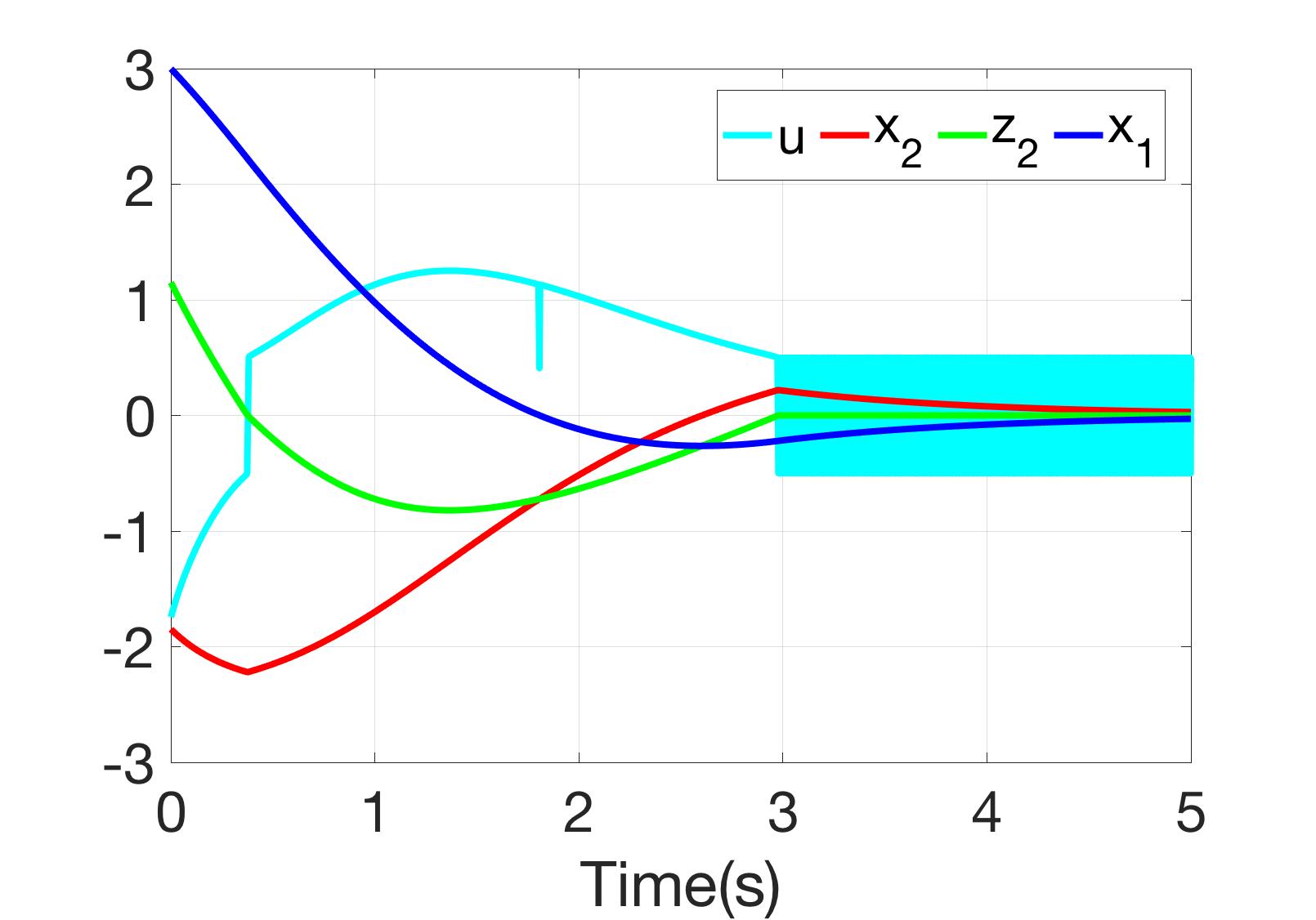
III-A Results with and with sign function
In this part, the controller (1) is applied to (4). The obtained results are depicted in Fig. 1. We can notice the very good performance of the proposed controller. The state converges to zero in a guaranteed-finite time. The same conclusion is stated for , which converges to zero in fixed-finite time. As is function of and , its convergence to zero is also achieved. For the behavior of the control (1), we can observe a chattering phenomena when at . This behavior is natural and can be explained by the fact the tower term in (1) goes to zero before the function , then the control will depend only on the sign function of . This behaviour appears briefly also before, mainly at when crosses zero and at when since the control depend also on the tower term . At these two instants the control (1) depends directly on the sign function, which explains these two briefly discontinuities of the control. To overcome this behavior, we propose to replace the discontinuous function of this control by a continuous one when and reaches zero. This introduces the next subsection.
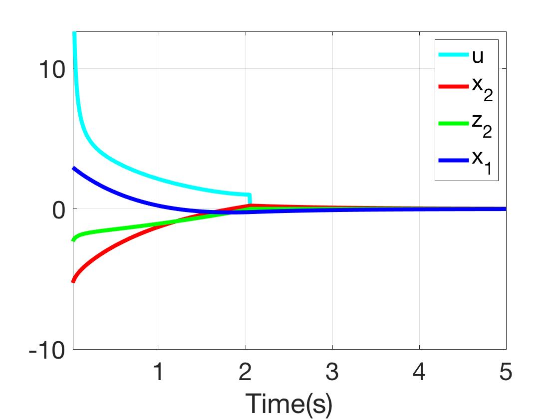
III-B Results with and with tanh function
In this part, the sign function used in (1) is replaced by the tanh function, where the gain of this function is fixed to to be more close to the behaviour of the sign function. The obtained results are depicted in Fig. 2. As excepted the same results about the guaranteed-finite time convergences of the states , and to zero are obtained. However, we can notice that the chattering disappeared in the control , thanks to the tanh function. However, as it can be seen on Fig. 2, the control needs more effort at initial conditions.
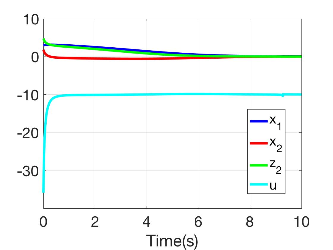
III-C Results with constant and with tanh function
In this part, we test the performances of the controller defined in (2) when it is applied to system (4) in presence of a constant bounded perturbation . We fixed (any another value can be chosen) and the simulation results are shown in (3). In Fig. 3 we can show that the control (2) performs well in the sense that the perturbation is exactly canceled ( in steady state) thanks to the integral term in (2). The latter is replaced by the tanh function with high gain (100000) to avoid chattering phenomenon. Even if the function is approximated by the function for avoiding the chattering, the convergence of the states and seems to be in guaranteed-finite time.
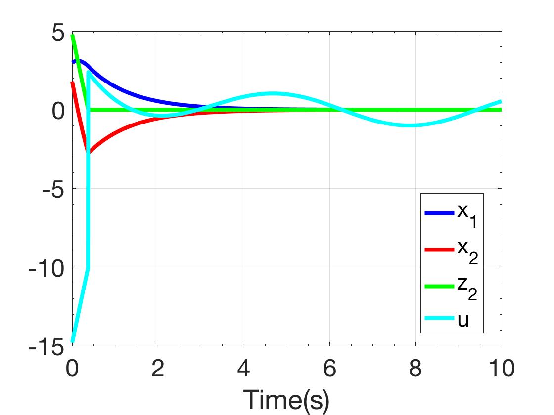
III-D Results with variable and with tanh function
In this part, we test the performances of the controller defined in (1) when it is applied to system (4) in presence of a variable bounded perturbation where its upper bound is known. For that we took as a sinus function: . The parameter of the control (1) is fixed to 10, i.e. , where is the upper bound of the sinus function. The obtained results, plotted in Fig. (4), show very good performances of the control (1), the perturbation is exactly canceled () thanks to the sign function in (2), which is replaced by tanh function to avoid chattering phenomenon. In this case the convergence of the states and are in finite time and not in guaranteed time for the function and only asymptotic for function.
IV Conclusion
In this paper, we propose a new control law on a power tower function truncated to order 2. This function makes it possible to use the backstepping technique in order to propose convergence in guaranteed and finite time. In a future work, the convergence finite times including the fixed one will be derived and the non-matching perturbations problem will be studied. The fixed-time will be assigned by the choice of some parameters and which multiply respectively the term and the term in the control design. Moreover, the approach will be extended to higher dimensional systems. In a second step, the behavior of such law in an observer-based control scheme or with respect to noisy measurements or actuator saturation or again under sampling must be investigated.
References
- [1] Vincent Andrieu, Laurent Praly, and Alessandro Astolfi. Homogeneous approximation, recursive observer design, and output feedback. SIAM Journal on control and optimization, 47(4):1814–1850, 2008.
- [2] G. Bornard and H. Hammouri. A high gain observer for a class of uniformly observable systems. In Proc. IEEE Conf. on Decision and Control CDC, pages 1494–1496, Brighton, England, 1991.
- [3] Emmanuel Cruz-Zavala and Jaime A Moreno. Homogeneous high order sliding mode design: a lyapunov approach. Automatica, 80:232–238, 2017.
- [4] R.A. Freeman and P.V. Kokotović. Backstepping design of robust controllers for a class of nonlinear systems. In M. FLIESS, editor, Nonlinear Control Systems Design 1992, IFAC Symposia Series, pages 431–436. Pergamon, Oxford, 1993.
- [5] L Fridman and A Levant. Higher order sliding modes. In Sliding mode control in engineering, pages 53–102. 2002.
- [6] M. Ghanes, J. P. Barbot, L. Fridman, A. Levant, and R. Boisliveau. A new varying-gain-exponent-based differentiator/observer: An efficient balance between linear and sliding-mode algorithms. IEEE Trans. on Automatic Control, 65(12):5407–5414, 2020.
- [7] Malek Ghanes, Jaime A Moreno, and Jean-Pierre Barbot. Arbitrary order differentiator with varying homogeneity degree. Automatica, 138:110111, 2022.
- [8] Hassan K Khalil. Nonlinear systems. 2002.
- [9] Hassan K Khalil and Laurent Praly. High-gain observers in nonlinear feedback control. International Journal of Robust and Nonlinear Control, 24(6):993–1015, 2014.
- [10] R. Arthur Knoebel. Exponentials reiterated. The American Mathematical Monthly, 88(4):235–252, 1981.
- [11] P Kokotovic, HK Khalil, and J O’Reilly. Singular perturbation methods in control: analysis and design, ser. Classics in applied mathematics. SIAM, (25), 1999.
- [12] P.V. Kokotovic, M. Krstic, and I. Kanellakopoulos. Backstepping to passivity: recursive design of adaptive systems. In [1992] Proceedings of the 31st IEEE Conference on Decision and Control, pages 3276–3280 vol.4, 1992.
- [13] Miroslav Krstic, Petar V. Kokotovic, and Ioannis Kanellakopoulos. Nonlinear and Adaptive Control Design. John Wiley & Sons, Inc., USA, 1st edition, 1995.
- [14] A. Levant. Sliding order and sliding accuracy in sliding mode control. Int. J. of Control, 58(6):1247–1263, 1993.
- [15] Yang Liu, Hongyi Li, Zongyu Zuo, Xiaodi Li, and Renquan Lu. An overview of finite/fixed-time control and its application in engineering systems, 2022.
- [16] Peter Lynch. The fractal boundary of the power tower function. In Nuno Silva, J. Recreational Mathematics Colloquium V: Proceedings of the Recreational Mathematics Colloquium V. Associacao Ludus, 2017.
- [17] A. Polyakov, D. Efimov, and W Perruquetti. Homogeneous differentiator design using implicit lyapunov function method. European Control Conference, IEEE, IFAC, pages –293288, 2014.
- [18] Andrey Polyakov. Generalized Homogeneity in Systems and Control. Springer-Verlag, Springer Nature Switzerland AG, 2020.
- [19] Andrey Polyakov, Denis Efimov, and Wilfrid Perruquetti. Finite-time and fixed-time stabilization: Implicit lyapunov function approach. Automatica, 51:332–340, 2015.
- [20] Lionel Rosier. Homogeneous lyapunov function for homogeneous continuous vector field. Systems & Control Letters, 19(6):467–473, 1992.
- [21] Sundarapandian Vaidyanathan and Ahmad Taher Azar, editors. Backstepping Control of Nonlinear Dynamical Systems. Advances in Nonlinear Dynamics and Chaos (ANDC). Academic Press, 2021.
- [22] A.N. Tikhonov. Systems of differential equations containing a small parameter in front of the derivatives. Mat. Sb., 31(3):575–586, 1952.
- [23] Vadim Utkin, Alex Poznyak, Yury Orlov, and Andrey Polyakov. Conventional and high order sliding mode control. Journal of the Franklin Institute, 357(15):10244–10261, 2020.
- [24] A. B. Vasileva and V. F. Butuzov. Singularly perturbed equations in critical cases. Moscow Izdatel Moskovskogo Universiteta Pt, January 1978.
- [25] Shijiao Wang, Chengming Jiang, Qunzhang Tu, and Changlin Zhu. Sliding mode control with an adaptive switching power reaching law. Sci Rep, 13, 2023.