Semi-Discrete Optimal Transport: Nearly Minimax Estimation With Stochastic Gradient Descent and Adaptive Entropic Regularization

Abstract

Optimal Transport (OT) based distances are powerful tools for machine learning to compare probability measures and manipulate them using OT maps. In this field, a setting of interest is semi-discrete OT, where the source measure $\mu$ is continuous, while the target $\nu$ is discrete. Recent works have shown that the minimax rate for the OT map is $\mathcal{O}(t^{-1/2})$ when using $t$ i.i.d. subsamples from each measure (two-sample setting). An open question is whether a better convergence rate can be achieved when the full information of the discrete measure $\nu$ is known (one-sample setting). In this work, we answer positively to this question by (i) proving an $\mathcal{O}(t^{-1})$ lower bound rate for the OT map, using the similarity between Laguerre cells estimation and density support estimation, and (ii) proposing a Stochastic Gradient Descent (SGD) algorithm with adaptive entropic regularization and averaging acceleration. To nearly achieve the desired fast rate, characteristic of non-regular parametric problems, we design an entropic regularization scheme decreasing with the number of samples. Another key step in our algorithm consists of using a projection step that permits to leverage the local strong convexity of the regularized OT problem. Our convergence analysis integrates online convex optimization and stochastic gradient techniques, complemented by the specificities of the OT semi-dual. Moreover, while being as computationally and memory efficient as vanilla SGD, our algorithm achieves the unusual fast rates of our theory in numerical experiments.

Keywords: Optimal Transport; Stochastic Gradient Descent; Statistical Estimation

1 Introduction

Optimal transport (OT) is now a widely used tool to compare probability distributions in different areas of data science such as machine learning (Courty et al., 2014; Genevay et al., 2018; Bigot et al., 2017), computational biology (Schiebinger et al., 2019), imaging (Feydy et al., 2017; Bonneel and Digne, 2023), even economics (Galichon, 2018) or material sciences (Buze et al., 2024). The computational and statistical efficiency of OT solvers is the key to facilitating their use in practical applications. Therefore, both computational methods and the statistical bottleneck in optimal transport (OT), often referred to as the curse of dimensionality, have received significant attention over the past decade (Peyré et al., 2019; Weed and Bach, 2017). Regularization such as Entropic OT (EOT) (Cuturi, 2013) is a popular method to alleviate these two issues. It consists of adding an entropic regularization term to the objective function. Annealing schemes on the regularization parameter to approximate the true solution of OT by its entropic approximation are efficient, as shown in (Kosowsky and Yuille, 1994; Schmitzer, 2019a; Feydy, 2020). Still largely open is the theoretical understanding of these methods (Sharify et al., 2011; Schmitzer, 2019a), which can shed light on the design of the annealing scheme, also called $\varepsilon$-scaling.

OT and its entropic regularization apply to different contexts of interest. The most general context is when the two distributions are accessed via samples and one wants to estimate the OT distance and the correspondence plan or map. Another context of interest in some applications is the case of semi-discrete OT, as in Kitagawa et al. (2016), in which one of the two distributions is discrete and the other continuous. This setting is slightly simpler than the general case since (i) the OT problem reduces to the estimation of Laguerre cells and (ii) the curse of dimensionality is alleviated (Pooladian et al., 2023).

Related works. In many applications of OT, one or both of the measures are accessed via i.i.d. samples. The goal then becomes to construct estimators of the OT map and/or cost. It is known that without any assumptions on the measures, the estimation of OT quantities suffers from the curse of dimensionality. For instance, estimating the Wasserstein distance from $t$ samples achieves a rate of $\mathcal{O}(t^{-\frac{1}{d}})$ for $d\geq 3$. Despite the curse of dimensionality, estimating OT quantities attracts a lot of interest. Relevant works include Fournier and Guillin (2015); Weed and Bach (2017); Chizat et al. (2020); Rigollet and Stromme (2022) for the OT cost, and Deb et al. (2021); Hütter and Rigollet (2021); Vacher et al. (2021); Pooladian et al. (2023) for the OT map.

We study here the estimation of OT quantities in the semi-discrete setting, where the continuous distribution is accessed through sampling, similarly to Mensch and Peyré (2020); Pooladian et al. (2023), but we assume full access to the discrete target measure, as in Genevay et al. (2016); Bercu and Bigot (2021). This setting is of interest since, as recently shown in Pooladian et al. (2023), the OT map estimation escapes the curse of dimensionality, even without assuming the map to be smooth or continuous. Indeed, they showed that a rate of $\mathcal{O}(t^{-\frac{1}{2}})$ is achievable in the ”one-sample” and ”two-sample” settings (sampling only from the source measure or from both measures). To do so, their work uses the EOT map estimator (Seguy et al., 2017; Pooladian and Niles-Weed, 2021) with a regularization $\varepsilon\asymp t^{-\frac{1}{2}}$, as well as results on the convergence rate of the entropic optimal potential to the Kantorovich potential in the semi-discrete setting proved in Altschuler et al. (2022); Delalande (2022). Moreover, they showed that the rate $\mathcal{O}(t^{-\frac{1}{2}})$ is minimax for the estimation of the OT map in the two-sample setting.

Beyond the statistical challenges, building efficient solvers for semi-discrete OT is also a considerable challenge. Many solvers of (E)OT in this setting are based on optimizing the semi-dual, which is a finite-dimensional convex optimization problem. In particular, efficient Newton and quasi-Newton methods (Mérigot, 2011; Lévy, 2015; Kitagawa et al., 2016) are proposed for low dimensions, employing meshes when the source density is known. For arbitrary dimensions, or when the source measure is only accessible via samples, Genevay et al. (2016) propose using semi-dual EOT and Stochastic Gradient Descent (SGD) based solvers as proxies for OT. The study of SGD and Averaged SGD (ASGD) for EOT was further investigated by Bercu and Bigot (2021), which notably demonstrated that the objective function is self-concordant and benefits from enhanced strong convexity near an optimum. Using these facts, Bercu and Bigot (2021) showed that a convergence rate of $\mathcal{O}(t^{-1})$ can be achieved for the squared Euclidean distance estimation of the discrete entropic optimal potential. However, terms in $\varepsilon^{-1}$ were considered negligible in their study, thus excluding small regularization.

Contributions. Our main contribution is twofold. First, we introduce an SGD-based algorithm to solve the semi-dual formulation of OT. This algorithm incorporates a projection step and an entropic regularization scheme that decreases with the number of samples. While being as computationally and memory efficient as vanilla SGD, our algorithm achieves enhanced convergence rates, thanks to the decreasing regularization. Specifically, given $t$ i.i.d. samples of the source measure, it achieves a convergence rate of $\mathcal{O}(t^{-2b})$ with $b\in(1/2,1)$ for both the discrete Kantorovich potential and OT cost estimation. We then construct an OT map estimator based on our discrete potential estimator and the closed form of the gradient of Fenchel transforms. By studying the difference between the Laguerre cells formed by the Kantorovich potential and our estimator, we retrieve a $\mathcal{O}(t^{-b})$ convergence rate for the OT map, for $b\in(1/2,1)$.

Second, building upon the parallel between measure support estimation and Laguerre cell estimations, we derive two new minimax lower bounds, characteristic of the fast rates of non-regular models: a $\mathcal{O}(t^{-2})$ rate for the Kantorovich potential and a $\mathcal{O}(t^{-1})$ rate for the OT map (compared to $\mathcal{O}(t^{-1/2})$ in the two-sample setting (Pooladian et al., 2023)). These lower bounds are nearly achieved by our estimators since $b<1$. Finally, we numerically showcase the convergence rates of our algorithm for the OT potential, map, and cost estimators.

Notations. We note $\|\cdot\|$ the euclidean norm, and for $\mathcal{C}\subset\mathbb{R}^{d}$, $D_{\mathcal{C}}:=\sup\{\|x-y\|:x,y\in\mathcal{C}\}$ denote its diameter. For $a,b\in\mathbb{R}$, $a\vee b:=\max\{a,b\}$ and $a\wedge b:=\min\{a,b\}$. For $v\in\mathbb{R}^{d}$, $v_{\min}:=\min_{1\leq j\leq d}v_{j}$. $\mathbf{1}_{d}$ and $\mathbf{0}_{d}$ denote the vectors $(1,\dots,1)$ and $(0,\dots,0)$ in $\mathbb{R}^{d}$. $\lambda_{\mathbb{R}^{d}}$ is the Lebesgue measure in $\mathbb{R}^{d}$. ${\mathcal{P}}(\mathbb{R}^{d})$ is the set of probabilities in $\mathbb{R}^{d}$, and for $\rho\in{\mathcal{P}}(\mathbb{R}^{d})$, $\mathrm{Supp}(\rho)$ is its support. $\mathcal{O}(\cdot)$ and $o(\cdot)$ are the usual approximation orders. We use $f\lesssim g$ if there exists a constant $C>0$ such that $f(\cdot)\leq Cg(\cdot)$. We write $a\asymp b$ if both $a\lesssim b$ and $b\lesssim a$.

2 Behind stochastic approximation for Optimal Transport

2.1 Background on (Entropic) Optimal Transport

Given a source and target probability measures $\mu,\nu\in{\mathcal{P}}(\mathbb{R}^{d})$, a cost function $c:\mathbb{R}^{d}\times\mathbb{R}^{d}\to\mathbb{R}^{+}$ and a regularization parameter $\varepsilon\geq 0$, the Entropic Optimal Transport (EOT) problem is

$$\mathrm{OT}_{c}^{\varepsilon}(\mu,\nu) :=\underset{\pi\in\Pi(\mu,\nu)}{\min}\int_{\mathbb{R}^{d}\times\mathbb{R}^{d}}c(x,y)\mathrm{d}\pi(x,y)+\varepsilon\int_{\mathbb{R}^{d}\times\mathbb{R}^{d}}\ln\left(\frac{\mathrm{d}\pi}{\mathrm{d}\mu\mathrm{d}\nu}(x,y)\right)\mathrm{d}\pi(x,y),$$ (1)

where $\Pi(\mu,\nu)$ is the set of joints probability measures on $\mathbb{R}^{d}\times\mathbb{R}^{d}$ with marginals $\mu$ and $\nu$. Mild conditions on $\mu,\nu$ and the cost can be made so that this problem is well-posed, see Villani (2009). When $\varepsilon=0$, Problem (1) recovers the Kantorovich formulation of OT. In this article, we focus on the quadratic cost $c(x,y)=\frac{1}{2}\|x-y\|^{2}$, although some of our results can be extended to more general costs. Our analysis relies on the semi-dual formulation of the convex problem (1) given by

$$\mathrm{OT}_{c}^{\varepsilon}(\mu,\nu) =\max_{f\in C(\mathbb{R}^{d})}\int_{\mathbb{R}^{d}}f(x)\mathrm{d}\mu(x)+\int f^{c,\varepsilon}(y)\mathrm{d}\nu(y),$$ (2)

where for all $y\in\mathbb{R}^{d}$,

$$f^{c,\varepsilon}(y): =\left\{\begin{array}[]{l}\min_{x\in\mathbb{R}^{d}}c(x,y)-f(x)\quad\text{ if }\quad\varepsilon=0,\\ -\varepsilon\log\left(\int_{\mathbb{R}^{d}}\exp\left(\frac{f(x)-c(x,y)}{\varepsilon}\right)\mathrm{d}\mu(x)\right)\quad\text{ if }\quad\varepsilon>0.\end{array}\right.$$

Under mild conditions on the cost or densities, a positive $\varepsilon$ makes the semi-dual formulation $\varepsilon^{-1}$-smooth (Cuturi and Peyré, 2018). The key property of this semi-dual formulation of (E)OT is to retain more convexity than the standard dual of (1) (see Hütter and Rigollet (2021); Vacher and Vialard (2023)).

Optimal maps and Brenier’s theorem. We consider the quadratic cost, $\varepsilon=0$ and $\mu,\nu$ having second-order moments. Under the additional assumption that the measure $\mu$ is absolutely continuous, the optimal potential $f^{*}$, called Kantorovich potential, is (locally) Lipschitz and the map

$$T_{\mu,\nu}(x)\coloneqq x-\nabla f^{*}(x)$$ (3)

pushes forward $\mu$ onto $\nu$ (see Brenier (1991)). In addition, $T_{\mu,\nu}$ is the gradient of a convex function. This optimal map has more importance than the OT cost in subfields of machine learning such as generative modeling (Khrulkov and Oseledets, 2022) or domain adaptation (Courty et al., 2017).

2.2 Semi-discrete OT

Semi-discrete (E)OT is when the source measure $\mu$ is absolutely continuous and the target measure $\nu=\sum_{j=1}^{M}w_{j}\delta_{y_{j}}$ is a finite sum of $M\geq 1$ Dirac masses with weights $w_{j}>0$. In this case, the semi-dual formulation reduces to a finite-dimensional convex optimization problem on $\mathbb{R}^{M}$

$$\min_{{\mathbf{g}}\in\mathbb{R}^{M}}H_{\varepsilon}(\mathbf{g})\stackrel{{\scriptstyle\text{ def. }}}{{=}}-\int_{\mathbb{R}^{d}}\mathbf{g}^{c,\varepsilon}(x)\mathrm{d}\mu(x)-\sum_{j=1}^{M}g_{j}w_{j}\,,$$ (4)

where for all $x\in\mathbb{R}^{d},\ {\mathbf{g}}^{c,\varepsilon}(x)$ is a (vectorial) $(c,\varepsilon)$-transform with respect to a vector ${\mathbf{g}}=(g_{1},\ldots,g_{M})\in\mathbb{R}^{M}$, defined by

$${\mathbf{g}}^{c,\varepsilon}(x) =\left\{\begin{array}[]{ll}\min_{j\in\llbracket 1,M\rrbracket}\left[\frac{1}{2}\|x-y_{j}\|^{2}-g_{j}\right]&\quad\text{ if }\quad\varepsilon=0,\\ -\varepsilon\ln\left(\sum_{j=1}^{M}\exp\left(\frac{-\frac{1}{2}\|x-y_{j}\|^{2}+g_{j}}{\varepsilon}\right)w_{j}\right)&\quad\text{ if }\quad\varepsilon>0.\end{array}\right.$$

The vector ${\mathbf{g}}$ corresponds to the value of the potential function at the points $y_{j}$. For notational convenience, we write $H_{\varepsilon}(\mathbf{g})=\int_{\mathbb{R}^{d}}h_{\varepsilon}(x,\mathbf{g})\mathrm{d}\mu(x)$ with $h_{\varepsilon}(x,\mathbf{g})=-\mathbf{g}^{c,\varepsilon}(x)-\sum_{j=1}^{M}g_{j}w_{j}$. For all $\mathbf{g}\in\mathbb{R}^{M}$ and given $X\sim\mu$, an unbiased estimator of the gradient is given by

$$\nabla_{\mathbf{g}}h_{\varepsilon}(X,\mathbf{g})_{j}=-w_{j}+\chi_{j}^{\varepsilon}(X,\mathbf{g}),\qquad 1\leq j\leq M\,,$$

where for $x\in\mathbb{R}^{d},{\mathbf{g}}\in\mathbb{R}^{M}$, we have

$$\chi_{j}^{\varepsilon}(x,{\mathbf{g}})=\frac{\exp\left(\frac{-\frac{1}{2}\|x-y_{j}\|^{2}+g_{j}}{\varepsilon}\right)w_{j}}{\sum_{k=1}^{M}\exp\left(\frac{-\frac{1}{2}\|x-y_{k}\|^{2}+g_{k}}{\varepsilon}\right)w_{k}}\cdot$$

For $\varepsilon=0$, $\chi_{j}(x,\mathbf{g})=\mathbb{1}_{\mathbb{L}_{j}({\mathbf{g}})}(x)$ is an indicator function and we have a partition $\mathbb{R}^{d}=\bigcup_{j=1}^{M}\mathbb{L}_{j}({\mathbf{g}})$, where for all $j\in\llbracket 1,M\rrbracket$,

$$\mathbb{L}_{j}({\mathbf{g}}):=\left\{x\in\mathbb{R}^{d};{\mathbf{g}}^{c}(x)=\frac{1}{2}\|x-y_{j}\|^{2}-g_{j}\right\}.$$

The convex sets $\mathbb{L}_{j}({\mathbf{g}})$ are called power or Laguerre cells and $\mu(\mathbb{L}_{i}({\mathbf{g}})\cap\mathbb{L}_{j}({\mathbf{g}}))=0$ when $i\neq j$. By the first-order optimality condition, solving semi-discrete OT amounts to finding ${\mathbf{g}}$ such that for all $j\in\llbracket 1,M\rrbracket$, $\mu(\mathbb{L}_{j}({\mathbf{g}}))=w_{j}$. Semi-discrete OT is a case of application of Brenier’s theorem. Given the optimal potential ${\mathbf{g}}^{*}$, the optimal map reads $\nabla({\mathbf{g}}^{*})^{c}(x)=x-y_{j}$ if $x$ is in the interior of $\mathbb{L}_{j}({\mathbf{g}}^{*})$.

2.3 Solving semi-discrete (E)OT with the semi-dual formulation

Exploiting its finite-dimensional nature, optimizing the OT semi-dual $H_{0}$ has become a popular approach. Notably, Newton and quasi-Newton methods are highly effective in scenarios with low dimensions and known source densities, utilizing meshes to approximate the source density (Mérigot, 2011; Lévy, 2015; Kitagawa et al., 2016). In scenarios involving arbitrary dimensions or when only sample-based access to the source measure is available, EOT emerges as a favored strategy. Notably, to avoid working with a discretized version of the source measure, such as with the Sinkhorn Algorithm, Genevay et al. (2016) recommend employing stochastic optimization to solve (4). Indeed, the semi-dual EOT problem has a convex objective of the form

$$H_{\varepsilon}({\mathbf{g}})=\mathbb{E}_{X\sim\mu}[h_{\varepsilon}(X,{\mathbf{g}})],$$

with $X$ as a random variable under $\mu$. As noted in Genevay et al. (2016), the main advantage of stochastic optimization algorithms is that they are suited for really large-scale problems, keeping in memory only the discrete measure $\nu$. Moreover, not relying on discretization permits an unbiased approach to solving the semi-discrete EOT problem.

For a given fixed regularization parameter $\varepsilon>0$, stochastic first-order methods are predominantly employed to solve (4). Starting with an initial value ${\mathbf{g}}_{0}\in\mathbb{R}^{M}$, these algorithms consider at each iteration one or many samples $X_{t}\sim\mu$ and rely on an update of the form

$${\mathbf{g}}_{t}={\mathbf{g}}_{t-1}-\gamma_{t}\nabla_{{\mathbf{g}}}h_{\varepsilon}(X_{t},{\mathbf{g}}_{t-1}).$$

At time $t$, the Averaged Stochastic Gradient Descent (ASGD) returns the averaged estimate $\mathbf{\overline{g}}_{t}=\frac{1}{t+1}\sum_{k=0}^{t}\mathbf{g}_{k}$, while Stochastic Gradient Descent (SGD) returns $\mathbf{g}_{t}$. ASGD, as an acceleration of SGD, has been widely studied in the literature (see Polyak and Juditsky (1992); Pelletier (2000); Bach and Moulines (2013), and Bercu and Bigot (2021) for the specific case of EOT).

Choosing the regularization parameter $\varepsilon$ for EOT. Approximating the EOT problem rather than the OT one benefits from an enhanced convergence rate, especially in the discrete setting. The introduction of the Sinkhorn Algorithm for solving the EOT problem, as highlighted by Cuturi (2013), has led to a resurgence of interest in OT within the Machine Learning community.

The choice of the regularization parameter $\varepsilon$ then becomes a practical and/or statistical problem:

1. In the discrete case, selecting the regularization parameter is a practical issue that aims to strike an optimal balance between convergence speed and accuracy (Cuturi, 2013; Dvurechensky et al., 2018). To address this trade-off, some heuristics, such as $\varepsilon$-scaling (Schmitzer, 2019b), which involves a decreasing regularization scheme, are employed, although they lack strong theoretical guarantees.

2. In the semi-discrete and continuous settings, the initial statistical problem is to determine the number of samples needed to accurately approximate the OT quantities. In this line of work, the use of EOT to construct estimators has also been proven to be satisfactory. In this case, studies show that regularization must decrease as the number of samples increases (Pooladian and Niles-Weed, 2021; Pooladian et al., 2023). However, discrete solvers do not adjust to the number of drawn points, as the solver is initiated once the points to approximate the measures have been sampled.

3 DRAG: Decreasing Regularization Averaged Gradient

3.1 Setting.

We focus here on the one-sample setting of semi-discrete OT. Specifically, we sample from the source measure $\mu$ and leverage the full information of the discrete measure $\nu$. Furthermore, fixing $R>0$ and $\alpha\in(0,1]$, we make the following mild assumption, already present in Delalande (2022); Pooladian et al. (2023).

Assumption 1.

Let $\mu\in{\mathcal{P}}(\mathbb{R}^{d})$, such that $\mathrm{Supp}(\mu)\subset B(0,R)$ and its density $d\mu$ is $\alpha$-Hölderian with, $0<\mathrm{d}\mu<\infty$ on its support. We note ${\mathcal{P}}_{\alpha}(B(0,R))$ the set of these measures.

The target measure $\nu$ is discrete, of the form $\nu=\sum_{j=1}^{M}w_{j}\delta_{y_{j}}$, with $\mathbf{w}=\left(w_{1},\ldots,w_{M}\right)$ its probability weights and $\left(y_{1},\ldots,y_{M}\right)\in B(0,R)^{M}$ its support.

3.2 DRAG: A gradient-based algorithm adaptive to both the samples size and regularization parameter

Having a regularization parameter $\varepsilon$ that decreases as the number of drawn samples increases is crucial to approximate the true OT cost and the Brenier map. However, no algorithm in the OT literature adapts to both entropic regularization and sample size simultaneously. In the discrete setting, the concept of decreasing regularization, known as $\varepsilon$-annealing (Schmitzer, 2019b), is recognized for accelerating the convergence of the Sinkhorn algorithm in practice. However, the sample size remains fixed. In contrast, SGD algorithms are inherently adaptive to the number of samples. Thus, we propose a decreasing sequence $(\varepsilon_{t})_{t}$ and suggest replacing the usual gradient step in ASGD with the following projected step with adaptive regularization

$$\mathbf{g}_{t}=\mathrm{Proj}_{\mathcal{C}}\left(\mathbf{g}_{t-1}-\gamma_{t}\nabla_{\mathbf{g}}h_{\varepsilon_{t-1}}(X_{t},\mathbf{g}_{t-1})\right),$$

where for $U\subset\mathbb{R}^{M}$ convex, we define the projector as $\mathrm{Proj}_{U}(\mathbf{g}):=\arg\min\{\|\mathbf{g}-\mathbf{g^{\prime}}\|,\mathbf{g^{\prime}}\in U\}.$ This method can be interpreted as a decreasing bias SGD scheme. For such a method, employing a projection step can be highly effective in ensuring convergence (Cohen et al., 2017; Geiersbach and Pflug, 2019). In the context of EOT, it is well established that the $(c,\varepsilon)$-transform enables the localization of a minimum of the semi-dual problem when the cost is bounded (Nutz and Wiesel, 2022). Specifically, since $\sup\{c(x,y_{j});x\in\mathrm{Supp}(\mu),j\in\llbracket 1,M\rrbracket\}<2R^{2}$ by Assumption 1, a preliminary projection set can be expressed as $\mathcal{C}_{\infty}:=[0,2R^{2}]^{M}.$ Nonetheless, leveraging the regularity of the cost function, we can have a projection set with a unique optimizer, as described in the following Lemma.

Lemma 1.

(Proof in Appendix B.7) Under Assumption 1, for all $\varepsilon\geq 0$, there exists a unique solution $\mathbf{g}^{*}_{\varepsilon}$ to (4) in $\mathcal{C}_{u}:=\{\mathbf{g}\in\mathbb{R}^{M}\ ;g_{1}=0\text{ and }|g_{j}|\leq R\|y_{1}-y_{j}\|,j\in\llbracket 1,M\rrbracket\}$.

Algorithm 1 DRAG

  Parameters: $(\gamma_{1},a,b,{\mathcal{C}})$

  Initialize $\mathbf{g}_{0}\in{\mathcal{C}}$, $\mathbf{\overline{{\mathbf{g}}}}_{0}=\mathbf{g}_{0}$, $\varepsilon_{0}=1$.

  for $k=1$ to $t$ do

     $\gamma_{k}=\gamma_{1}k^{-b}$

     $X_{k}\sim\mu$

     $\mathbf{g}_{k}\!=\!\mathrm{Proj}_{\mathcal{C}}\left(\mathbf{g}_{k-1}-\!\gamma_{k}\nabla_{\mathbf{g}}h_{\varepsilon_{k-1}}(X_{k},\mathbf{g}_{k-1}\!)\right)$

     $\mathbf{\overline{{\mathbf{g}}}}_{k}=\frac{1}{k+1}\mathbf{g}_{k}+\frac{k}{k+1}\mathbf{\overline{{\mathbf{g}}}}_{k-1}$

     $\varepsilon_{k}=k^{-a}$

  end for

  return $\mathbf{\overline{{\mathbf{g}}}}_{t}$

Note that the choice $g_{1}=0$ is arbitrary. In what follows, we refer to ${\mathcal{C}}={\mathcal{C}}_{\infty}$ or ${\mathcal{C}}={\mathcal{C}}_{u}$ as our projection set. Note that for both set, the projection is nearly cost-free, as it involves merely clipping each coordinate of our vector.

Finally, in order to accelerate the convergence, we consider the Decreasing Regularization projected Averaged stochastic Gradient descent (DRAG) defined by

$$\overline{{\mathbf{g}}}_{t}=\frac{1}{t+1}{\mathbf{g}}_{t}+\frac{t}{t+1}\overline{{\mathbf{g}}}_{t-1},$$

with $\overline{{\mathbf{g}}}_{0}={\mathbf{g}}_{0}$. The pseudo-code of our algorithm is given in Algorithm 1. A main advantage of DRAG is that it has a $\mathcal{O}(dtM)$ computational complexity and $\mathcal{O}(dM)$ spatial complexity.

3.3 Convergence rate before averaging

As a key step to the convergence rate of DRAG, we will provide the convergence rate of the non averaged estimate ${\mathbf{g}}_{t}$ to ${\mathbf{g}}_{\varepsilon_{t}}^{*}$, solving (4) with regularization $\varepsilon_{t}$. Note that, up to a transformation of the form $\mathbf{g}_{\varepsilon_{t}}^{*}+a\mathbf{1}_{M}$, where $a\in\mathbb{R}^{*}$, the minimizer of the semi-dual is unique. Consequently, no matter the set ${\mathcal{C}}$ chosen, we focus our analysis on the orthogonal complement of the subspace spanned by $\mathbf{1}_{M}$, denoted as $\mathrm{Vect}(\mathbf{1}_{M})^{\bot}$. For simplicity, for ${\mathbf{g}},{\mathbf{g}}^{\prime}\in\mathbb{R}^{M}$, we denote for $p\in[1,\infty]$

$$\|{\mathbf{g}}-{\mathbf{g}}^{\prime}\|_{p}:=\|{\mathbf{g}}-{\mathbf{g}}^{\prime}\|_{p\ \mathrm{Vect}(\mathbf{1}_{M})^{\bot}}\,,\qquad\langle{\mathbf{g}},{\mathbf{g}}^{\prime}\rangle:=\langle{\mathbf{g}},{\mathbf{g}}^{\prime}\rangle_{\mathrm{Vect}(\mathbf{1}_{M})^{\bot}}\,.$$

Our analysis is greatly influenced by the findings in Corollary 2.2 from Delalande (2022), which states that for $0\leq\varepsilon^{\prime}\leq\varepsilon$, under Assumption 1 with $\mu\in{\mathcal{P}}_{\alpha}(B(0,R))$, for any $\alpha^{\prime}\in(0,\alpha)$, there exists a constant $K_{0}$, notably depending on the caracterstics of $\nu$ (see Delalande (2022)), such that

$$\left\|{\mathbf{g}}_{\varepsilon}^{*}-{\mathbf{g}}^{*}_{\varepsilon^{\prime}}\right\|\leq K_{0}\varepsilon^{\alpha^{\prime}}\left(\varepsilon-\varepsilon^{\prime}\right).$$ (5)

In addition, the convergence rates of our algorithm take advantage of the two following properties of the entropic semi-dual. For any $\varepsilon>0$, noting $w_{\min}:=\min_{j\in\llbracket 1,M\rrbracket}w_{j}$,

• $H_{\varepsilon}$ is locally strongly convex on $\mathrm{Vect}(\mathbf{1}_{M})^{\bot}$ and the smallest eigenvalue of its Hessian at $g_{\varepsilon}^{*}$ on $\mathrm{Vect}(\mathbf{1}_{M})^{\bot}$ is greater than $w_{\min}\varepsilon^{-1}$ (Bercu and Bigot (2021), Lemma A.1).

• $H_{\varepsilon}$ is $\frac{1}{\varepsilon}$-self concordant (Bercu and Bigot (2021), Lemma A.2).

Let us emphasize that, surprisingly, the first point reveals that the strong convexity at the optimum increases as we decrease the parameter $\varepsilon$. By combining these two points and benefiting from our projection step, we derive the following lemma.

Lemma 2.

(Proof in Appendix 2) For all regularization $\varepsilon>0$ and for all ${\mathbf{g}}\in\mathcal{C}$, we have

$$\left\|\nabla H_{\varepsilon}({\mathbf{g}})-\nabla^{2}H_{\varepsilon}\left({\mathbf{g}}_{\varepsilon}^{*}\right)\left({\mathbf{g}}-{\mathbf{g}}_{\varepsilon}^{*}\right)\right\|\leq\frac{4}{\varepsilon}\|{\mathbf{g}}-{\mathbf{g}}_{\varepsilon}^{*}\|_{\infty}^{2}.$$ (6)

Moreover, defining $K_{\mathbf{w}}:=2w_{\min}^{-1}\max\{2R^{2},1\}$ and $A_{{\mathbf{g}},\varepsilon}:=1-e^{-\frac{2}{\varepsilon}\left[1\wedge\|{\mathbf{g}}-{\mathbf{g}}_{\varepsilon}^{*}\|\right]}$, we have

$$\left\langle\nabla H_{\varepsilon}({\mathbf{g}}),{\mathbf{g}}-{\mathbf{g}}_{\varepsilon}^{*}\right\rangle\geq\frac{A_{{\mathbf{g}},\varepsilon}}{K_{\mathbf{w}}}\|{\mathbf{g}}-{\mathbf{g}}_{\varepsilon}^{*}\|^{2}.$$ (7)

While technical, this lemma is a key step for our convergence guarantees and thus warrants further discussion. Note that $A_{{\mathbf{g}},\varepsilon}/K_{\mathbf{w}}$ can be interpreted as a form of local strong convexity coefficient of $H_{\varepsilon}$. However, if $\|{\mathbf{g}}-{\mathbf{g}}_{\varepsilon}^{*}\|/\varepsilon$ is small, the term $A_{{\mathbf{g}},\varepsilon}$ tends to 0, and we would not be able to exploit more local strong convexity. This situation is unavoidable with any fixed regularization $\varepsilon$, if convergence to ${\mathbf{g}}_{\varepsilon}^{*}$ is desired. The use of a decreasing regularization scheme helps to avoid this problem. Indeed, if the term $A_{{\mathbf{g}}_{t},\varepsilon_{t}}$ remains small for any $t$ and $\varepsilon_{t}$ tends to 0, then $\|{\mathbf{g}}_{t}-{\mathbf{g}}_{\varepsilon_{t}}^{*}\|$ also tends to 0. However, if at time $t$, $A_{{\mathbf{g}}_{t},\varepsilon_{t}}$ is close to 1, we can exploit strong convexity. Thus, a decreasing regularization scheme ensures good convergence behavior, regardless of $A_{{\mathbf{g}}_{t},\varepsilon_{t}}$. Building on these essential properties, we obtain the convergence rate for the non-averaged iterates of DRAG.

Theorem 1.

(Proof in Appendix B.1) Under Assumption 1 with $\mu\in{\mathcal{P}}_{\alpha}(B(0,R))$, taking the parameters $(\gamma_{1},a,b)$ of DRAG such that $\gamma_{1}>0,\ 1+a+a\alpha>2b,\ a\geq\frac{b}{2}$ and $b\in\left(\frac{1}{2},1\right)$, we have

$$\mathbb{E}\left[\|{\mathbf{g}}_{t}-{\mathbf{g}}_{\varepsilon_{t}}^{*}\|^{2p}\right] \lesssim\frac{1}{w_{\min}^{p}t^{bp}},\qquad t\geq 1,\ p\in\{1,2\}.$$

Remarkably, we achieve a convergence rate without any undesirable dependence on regularization. Our projection step and the improvements in Lemma 2, compared to Lemma A.1 in Bercu and Bigot (2021), were crucial for this achievement. In contrast, Bercu and Bigot (2021) derived a convergence rate of the form $\mathcal{O}(\varepsilon^{-c}t^{-b})$ for a fixed regularization, with $c$ at least equal to $1$. Note that having no adverse dependence on the regularization parameter is essential for our algorithm, as it (i) employs a decreasing regularization scheme and (ii) aims to leverage the increased strong convexity at the optimum as $\varepsilon_{t}$ decreases. This last point will be further discussed in the next section.

3.4 Acceleration and quadratic convergence rate for DRAG

In convex stochastic optimization, it is known that averaging SGD iterations can lead to acceleration. More precisely, ASGD can adapt to the possibly unknown local strong convexity of the objective function at the optimizer (Bach, 2014). As we saw previously, the strong convexity of $H_{\varepsilon}$ increases as the regularization parameter $\varepsilon$ decreases. Despite the fact that our objective function changes at each time $t$, Theorem 2 (Proof in Appendix B.2) shows that DRAG fully exploits the increase in local strong convexity.

Theorem 2.

(Proof in Appendix B.2) Under the same assumptions as in Theorem 1, taking $a\geq b$,

$$\mathbb{E}[\|\overline{{\mathbf{g}}}_{t}-{\mathbf{g}}^{*}\|^{2}] \lesssim\frac{1}{w_{\min}^{4}t^{2b}}\,,\qquad t\geq 1\,.$$

Note that as $b$ tends to $1$, we achieve a quadratic convergence rate. We emphasize that this convergence rate is surprising, since for a general strongly convex function, the expected convergence rate would typically be linear. This difference comes from the fact that we face a Laguerre cells support problem. In parametric statistics, support problems are known to often be non regular and can yield an enhanced quadratic convergence rate (see, for instance, Wainwright (2019), Chapter 15). In the next theorem, we show that our convergence rate to ${\mathbf{g}}^{*}$ is nearly minimax.

Theorem 3.

(Proof in Appendix B.5) Let $\nu\in{\mathcal{P}}(\mathbb{R})$ be a fixed discrete measure of $M$ points. Then,

$$\inf_{{\mathbf{g}}^{(t)}}\sup_{\mu\in{\mathcal{P}}_{\alpha}(B(0,R))}\mathbb{E}\left[\|{\mathbf{g}}^{(t)}-{\mathbf{g}}^{*}\|^{2}\right]\gtrsim\frac{M}{t^{2}},$$

where ${\mathbf{g}}^{*}$ is the discrete optimal vector, solving the non regularized semi-dual in (4). The infimum is taken over all vectors ${\mathbf{g}}^{(t)}\in\mathbb{R}^{M}$ constructed using $t\in\mathbb{N}^{*}$ i.i.d samples of $\mu$.

Remark: While the dependence on $w_{\min}$ (or $M$) may seem minor in our context since it is a constant, we have included it in our analysis. This is pertinent, especially when applying DRAG to a discretized version of a continuous measure, which could result in a large $M$. We highlight that such results, demonstrating explicit dependence on the weights or number of points, are novel in the semi-discrete optimal transport (OT) literature. Additionally, when the weights of the discrete measure are uniform, our analysis achieves a convergence rate closer to $\mathcal{O}(M^{2}t^{-2b})$ (refer to the proof of Theorem 2 for further details). We believe that a theoretical convergence rate of $\mathcal{O}(w_{\min}^{-2}t^{-2b})$ is achievable for DRAG. Indeed, a quadratic dependence on the strong-convexity coefficient is commonly observed in ASGD (Bach, 2014). This dependence is illustrated in Figure 4.

4 Optimal Transport cost and Brenier map estimation rate with DRAG

4.1 OT and EOT cost estimation

In this part, we derive convergence rates of the (E)OT costs using DRAG.

Corollary 1.

(Proof in Appendix B.3) Taking the same assumptions as Theorem 2, with $0<\varepsilon<1$ and $0<\alpha^{\prime}<1$, we have the following convergence rate for the approximation of the (E)OT costs

$$\mathbb{E}\left|H_{\varepsilon}({\mathbf{g}}^{*}_{\varepsilon})-H_{\varepsilon}(\overline{{\mathbf{g}}}_{t})\right| \lesssim\varepsilon^{2\alpha^{\prime}-1}(\varepsilon-\varepsilon_{t})^{2}+\frac{1}{\varepsilon t^{2b}},$$ (8)

$$\mathbb{E}\left|H_{0}({\mathbf{g}}^{*})-H_{0}(\overline{{\mathbf{g}}}_{t})\right| \lesssim\frac{1}{t^{2b}}.$$ (9)

Once again, we achieve a superior rate compared to the typical $\mathcal{O}(t^{-1})$ observed in strongly convex and/or smooth scenarios, highlighting that semi-discrete OT deviates from conventional problems. Interestingly, while $H_{\varepsilon_{t}}(\overline{{\mathbf{g}}}_{t})$ could approximate the OT cost, this estimator worsens in convergence rate as $\varepsilon_{t}$ decreases. Here, the regularization parameter $\varepsilon$ introduces a trade-off, necessitating a balance between convergence rate and precision. Conversely, for OT, we exploit the consistent smoothness of $H_{0}$ (as noted in Theorem 4.1, Kitagawa et al. (2019)), which allows us to derive our asymptotic result without such a trade-off.

4.2 Brenier map estimation

When employing entropic regularization, a popular choice involves using the estimator of the entropic Brenier map

$$T_{\mu,\nu}^{\varepsilon}({\mathbf{g}}_{\varepsilon}^{*})(x)=x-\nabla({\mathbf{g}}_{\varepsilon}^{*})^{c,\varepsilon}.$$ (10)

Indeed, for $\hat{{\mathbf{g}}}\in\mathbb{R}^{M}$, $T_{\mu,\nu}^{\varepsilon}(\hat{{\mathbf{g}}})(x)$ could serve as an estimator. The objective is then to find an accurate estimator, $\hat{{\mathbf{g}}}$, close to ${\mathbf{g}}_{\varepsilon}^{*}$, and to analyze its performance based on the bias-variance decomposition

$$\|T_{\mu,\nu}-T_{\mu,\nu}^{\varepsilon}(\hat{{\mathbf{g}}})\|_{L^{2}(\mu)}^{2} \lesssim\|T_{\mu,\nu}^{\varepsilon}(\hat{{\mathbf{g}}})-T_{\mu,\nu}^{\varepsilon}({\mathbf{g}}_{\varepsilon}^{*})\|_{L^{2}(\mu)}^{2}+\varepsilon,$$

using the fact that $\|T_{\mu,\nu}-T_{\mu,\nu}^{\varepsilon}({\mathbf{g}}_{\varepsilon}^{*})\|_{L^{2}(\mu)}^{2}\lesssim\varepsilon$ (Pooladian et al. (2023), Theorem 3.4). However, the mapping ${\mathbf{g}}\mapsto T_{\mu,\nu}^{\varepsilon}({\mathbf{g}})$ is $\varepsilon^{-1}$-Lipschitz, complicating the bias-variance trade-off given that $\varepsilon_{t}=t^{-b}$. Instead, we rely on the gradient computed thanks to the $c$-transform of the estimator $\overline{{\mathbf{g}}}_{t}$ of DRAG. In fact, for any $x\in\mathbb{R}^{d}$, if there exists $j\in\llbracket 1,M\rrbracket$ such that $x$ is in the interior of $\mathbb{L}_{j}({\mathbf{g}}^{*})\cap\mathbb{L}_{j}(\overline{{\mathbf{g}}}_{t})$, we have

$$T_{\mu,\nu}(x)=x-\nabla(\overline{{\mathbf{g}}}_{t})^{c}(x).$$

Indeed, no matter ${\mathbf{g}}$, as soon as $x\in\mathbb{R}^{d}$ is in the interior of $\mathbb{L}_{j}({\mathbf{g}})$, the gradient of ${\mathbf{g}}^{c}$ is given by

$$\nabla({\mathbf{g}})^{c}(x)=\arg\max_{k}\left\{\frac{1}{2}\|x-y_{k}\|^{2}-g_{j}\right\}=y_{j}.$$ (11)

By analyzing the differences of Laguerre cells partitions between $\mathbb{L}(\overline{{\mathbf{g}}}_{t})$ and $\mathbb{L}({\mathbf{g}}^{*})$, we derive the following theorem.

Theorem 4.

(Proof in Appendix B.4) Under the same assumptions as Theorem 1, defining for all $x\in\mathbb{R}^{d}$ and time $t\geq 0$ $T(\overline{{\mathbf{g}}}_{t})(x)=x-\nabla\overline{{\mathbf{g}}}_{t}^{c}$, we have for all $1\leq p<\infty$ the convergence rate

$$\mathbb{E}\left[\|T_{\mu,\nu}-T_{\mu,\nu}(\overline{{\mathbf{g}}}_{t})\|_{L^{p}(\mu)}^{p}\right]\lesssim\frac{1}{t^{b}}.$$

Minimax estimation. In the two-sample setting, where we subsample from both $\mu$ and $\nu$, Pooladian et al. (2023) shows that a convergence rate of $\mathcal{O}(t^{-1/2})$ is minimax for the squared $L^{2}$ error of the Brenier map estimation. As we see in Theorem 4, this rate can be improved to $\mathcal{O}(t^{-1})$ in the one-sample setting, as $b$ tends to 1. In the following theorem, we prove that this rate is minimax.

Theorem 5.

(Proof in Appendix B.6) Under the assumptions of Theorem 2, for any $p\in[1,\infty[$,

$$\inf_{T^{(t)}}\sup_{\mu\in{\mathcal{P}}_{\alpha}(B(0,R))}\mathbb{E}\left[\|T_{\mu,\nu}-T^{(t)}\|_{L^{p}(\mu)}^{p}\right]\gtrsim\frac{1}{t},$$

where the infimum is taken over all maps $T^{(t)}$ constructed using $t\in\mathbb{N}^{*}$ iid samples of $\mu$.

5 Numerical experiments

In this section, we numerically verify our convergence rate guarantees through various examples. For each example, we know the theoretical OT map, cost, and discrete potential. The first two examples are similar to those in Pooladian et al. (2023). In all figures, we fixed the parameters of DRAG to $(\gamma_{1}=\sqrt{w_{\min}},a=b=0.75)$. While increasing $b$ leads asymptotically to a better convergence rate, it decreases the step size of our gradient descent. Therefore, we need to wait longer to observe the acceleration from averaging. Our numerical investigation found that our parameter selection achieves a good compromise between convergence rate and the time before acceleration and is robust without further hypertuning.

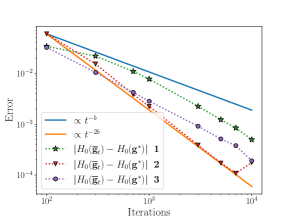
Figure 1: Cost error evolution through iterations, approximated with $10^{7}$ Monte Carlo samples, for Examples 1,2 and 3.

Examples settings: (1) $\mu\sim\mathcal{U}([0,1]^{10})$, $\mathrm{Supp}(\nu)=\{y_{j}=(\frac{j-1/2}{J},\frac{1}{2},...,\frac{1}{2}),j\in\llbracket 1,100\rrbracket\}$, $\mathbf{w}=\frac{1}{100}\mathbf{1}_{100}$. (2) $\mu\sim\mathcal{U}([0,1]^{10})$, $M=30$ and $y_{1},...,y_{M}$ randomly generated in $[0,1]^{10}$ . We then also randomly generate $g^{*}\in\mathbb{R}^{30}$ and approximate $\mathbf{w}$ with Monte Carlo (MC) , such that $g^{*}$ is the discrete optimum potential. This setting led to $w_{\min}=0.00103$. (3) $\mu\sim\mathcal{U}([\delta,1+\delta])$, $\delta=0.5$, $\mathrm{Supp}(\nu)=\left\{\frac{k}{M};k\in\llbracket 1,M\rrbracket\right\}$, $\mathbf{w}=\frac{1}{M}\mathbf{1}_{M},M=1000$. While in dimension 1, this example is interesting since it appears in the proofs of Theorem 3 and 5.

OT cost, map and potential convergence.

In Figures 1 and 2, we show the convergence rates of the OT cost, map, and discrete potential. As we can see, we match our theoretical rates perfectly, except for the OT cost, where the rates are slightly slower. This discrepancy could be due to (i) our results for the OT cost estimations being asymptotic and (ii) our OT cost estimation already being extremely precise, with $10^{7}$ MC samples proving insufficient to achieve precision around $5\cdot 10^{-4}$.

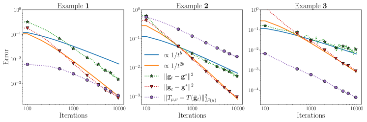
Figure 2: Convergence rate of our discrete potential and map estimators for Examples 1,2 and 3.

Visualisation of the OT map estimators with DRAG.

We visualize our OT map estimator $T(\overline{{\mathbf{g}}}_{t})=x-\nabla(\overline{{\mathbf{g}}}_{t})^{c}$ on a concrete example of Monge-Kantorovich (MK) quantiles (Chernozhukov et al., 2017). In this context, having a target measure $\nu$ to investigate, the source measure is set to be the uniform measure on the unit Euclidean ball $\mu\sim\mathcal{U}(B(0,1))$. The goal is then to visualize the destinations through the OT map of points in regions $B(0,(k+1)/10)\setminus B(0,k/10)$ for $k\in\llbracket 0,9\rrbracket$, which define MK quantile regions. We used $M=10^{5}$ points to approximate $\nu$, a discrete version of a boomerang-shaped measure. Finally, we launched DRAG with $t$ iterations. In Figure 3, we present the estimated MK quantiles regions of $\nu$, where each color represents a region, starting from $B(0,0.1)$ in the center. In this example, taking $t=10^{7}$ samples was sufficient and produced a similar result to when more samples were used.

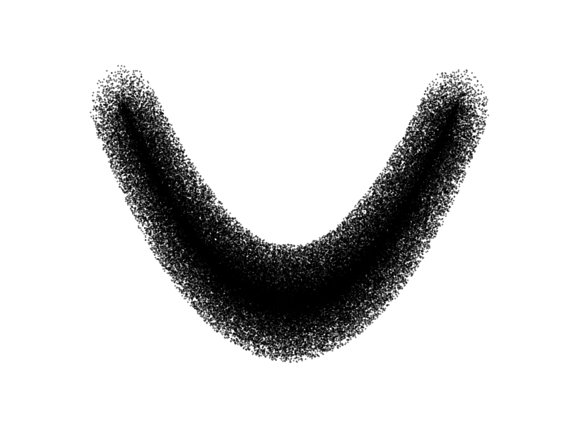
(a) Target measure

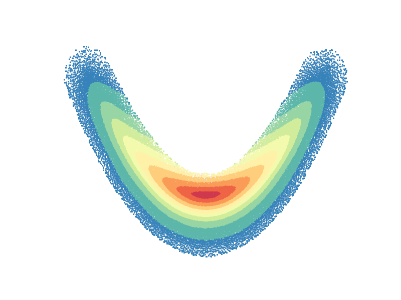
(b) OT map approx.

Figure 3: MK Regions and OT map approximation with DRAG.

Dependence of our convergence rate as $M$ grows.

As discussed in Section 3.4, our theoretical analysis indicates a dependence on $w_{\min}^{4}$. In examples 1 and 3, where similar problems arise with increased point counts, we run our algorithm with progressively larger $M$ and $M^{2}$ iterations. Our theory predicts that the error of the estimator ${\mathbf{g}}_{t}$ should decrease linearly, yet if the dependence of DRAG is indeed on $w_{\min}^{4}$, the error would increase quadratically, or remain constant if the actual dependence is $w_{\min}^{2}$. As illustrated in Figure 4, our theoretical bound accurately matches the behavior of $\|{\mathbf{g}}_{t}-{\mathbf{g}}^{*}\|^{2}$. Moreover, the behavior of $\|\overline{{\mathbf{g}}}_{t}-{\mathbf{g}}^{*}\|^{2}$ suggests that our theoretical bound may not be sharp, as discussed after Theorem 2.

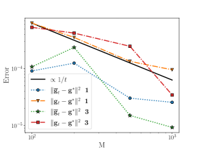
Figure 4: Error evolution of DRAG for ${\mathbf{g}}_{t}$ and $\overline{{\mathbf{g}}}_{t}$ as $M$ grows, for Examples 1 and 3, $t=M^{2}$ iterations.

Further experiments. In the appendix, we present additional experiments that, while not altering our theoretical findings, could be highly beneficial for practitioners. Specifically, we provide evidence that mini-batching with GPU computation and weighted averaging of the iterates $\mathbf{g}_{t}$ can significantly accelerate the algorithm. We also briefly discuss the choice of the parameters $a$ and $b$ and compare DRAG with SGD and ASGD.

6 Conclusion

In EOT, a decreasing regularization parameter naturally appeals to practitioners who aim to speed up Sinkhorn-like algorithms with an annealing scheme. Similarly, in the statistical community, a regularization that decreases with the number of points is favored to more accurately approximate true OT quantities. With our algorithm, DRAG, we demonstrate that these two motivations for decreasing regularization can coexist successfully. Moreover, we derive two new minimax lower bound theorems to approximate OT quantities in the one-sample setting of semi-discrete OT and show that DRAG nearly achieves these bounds.

Our algorithm nearly achieves the minimax rate when $b$ is close to 1. However, the closer $b$ is to 1, the higher the constants in the rates. In practice, the choice $a=b\approx 0.75$ gives robust practical results, as shown in Figure 7 in the appendix. An open direction is to design an improvement of our DRAG algorithm that achieves the minimax lower bound, while not suffering from large multiplicative constants, and remaining as computationally and memory efficient as our algorithm.

Our results can also motivate further investigation into different lines of work: (i) Studying the convergence of the discrete potential in semi-discrete OT for different costs. Indeed, the main challenge in extending the convergence proof of our algorithm to other costs is obtaining results similar to those in (Delalande (2022), Corollary 2.2) for alternative cost functions. (ii) Developing decreasing regularization algorithms in the continuous case to efficiently approximate OT distances and maps. (iii) Adapting our approach to demonstrate or improve the acceleration of entropic annealing schemes for EOT solvers in the discrete case.

Appendix

Appendix A Additional experiments

Weighted Averaging: Maintaining a better trade-off between averaged and non-averaged iterations.

Since the dependence of DRAG iterates $\overline{{\mathbf{g}}}_{t}$ on the number of points $M$ is at least quadratic, whereas for the non-averaged iterates ${\mathbf{g}}_{t}$ it is only linear, when the total number of iterations $t$ is insufficient (i.e., $t\leq M^{2}$), ${\mathbf{g}}_{t}$ can outperform $\overline{{\mathbf{g}}}_{t}$ as an estimator. One strategy to try to consistently achieve the best estimator regardless of the time $t$ is through weighted averaging Mokkadem and Pelletier [2011].

Namely, we replace the averaged estimator $\overline{{\mathbf{g}}}_{t}=\frac{1}{t+1}\sum_{k=0}^{t}{\mathbf{g}}_{t}$, by

$$\overline{{\mathbf{g}}}_{t}^{(\omega)}:=\frac{1}{\sum_{k=0}^{t}\log(k+1)^{\omega}}\sum_{k=0}^{t}\log(k+1)^{\omega}{\mathbf{g}}_{k},$$

with a parameter $\omega>0$. The parameter $\omega$ balances the weights assigned to the estimators ${\mathbf{g}}_{k}$. As $\omega$ increases, greater importance is given to the more recent estimates, while we retrieve $\overline{{\mathbf{g}}}_{t}$ when $\omega$ goes to $0$. As for the usual averaged estimators, we can perform the weighted average online, without having to store all the iterates, with the recursion

$$\overline{{\mathbf{g}}}_{t+1}^{(\omega)}=\left(1-\frac{\ln(t+1)^{\omega}}{\sum_{k=0}^{t}\ln(k+1)^{\omega}}\right)\overline{{\mathbf{g}}}_{t}^{(\omega)}+\frac{\ln(t+1)^{\omega}}{\sum_{k=0}^{t}\ln(k+1)^{\omega}}{\mathbf{g}}_{t+1}.$$

It is important to note that $\overline{{\mathbf{g}}}_{t}^{(\omega)}$ will have the same asymptotic convergence guarantees as $\overline{{\mathbf{g}}}_{t}$.

In the following experiments, we operate under conditions where the number of iterations $t$ is insufficient for the estimator $\overline{{\mathbf{g}}}_{t}$ to outperform ${\mathbf{g}}_{t}$. We set $M=1000$ in Examples 1 and 3, select $\omega=2$ for the weighted average parameter, and fix $t$ at $10^{5}$.

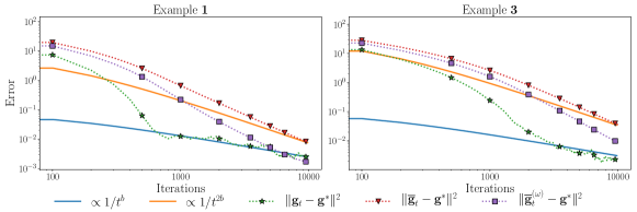
Figure 5: Comparison between ${\mathbf{g}}_{t},\overline{{\mathbf{g}}}_{t}$ and $\overline{{\mathbf{g}}}_{t}^{(\omega)}$ on Examples 1 and 3, fixing $M=1000$ and $\omega=2$.

As illustrated in Figure 5, the estimator ${\mathbf{g}}_{t}$ begins to converge after approximately $M$ iterations and remains superior to $\overline{{\mathbf{g}}}_{t}$ throughout the figure, since we are still within the regime where $t\leq M^{2}$. However, we see that the weighted average estimator $\overline{{\mathbf{g}}}_{t}^{(\omega)}$ consistently outperforms $\overline{{\mathbf{g}}}_{t}$ and already surpasses ${\mathbf{g}}_{t}$ in performance after $10^{5}$ iterations in Example 1.

Mini-batch DRAG.

As for Vanilla SGD, we can take advantage of GPU parallelization and replace the gradient estimator using one sample $X\sim\mu$

$$\nabla_{{\mathbf{g}}}h_{\varepsilon}(X,{\mathbf{g}})$$

by a mini-batch estimator, using $n_{b}\geq 1$ i.i.d samples $X_{1},...,X_{n_{b}}$ samples of the source measure at once

$$\frac{1}{n_{b}}\sum_{k=0}^{n_{b}}\nabla_{{\mathbf{g}}}h_{\varepsilon}(X_{k},{\mathbf{g}}).$$ (12)

Of course, no matter the choice $n_{b}$, (12) defines an unbiased estimator of $\nabla H_{\varepsilon}({\mathbf{g}})$.

Using a mini-batch of size $n_{b}$, we suggest multiplying $\gamma_{1}$ by $\sqrt{n_{b}}$, as is usual with mini-batch SGD. The following figure shows the acceleration due to mini-batching in Example 2, while maintaining the same computational time when using a GPU. Indeed, each mini-batch estimator has an error an order of magnitude lower than the non-batched ones, even with a small mini-batch size of $n_{b}=16$.

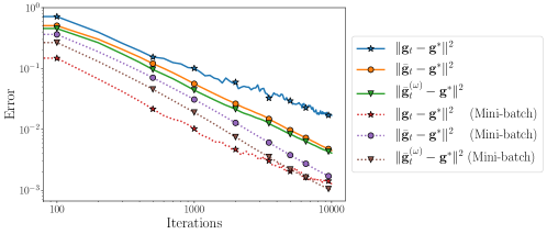
Figure 6: Comparison of the non mini-batched and mini-batched estimators on Example 2, $n_{b}=16$.

Influence of the parameter $a$ and $b$.

In Figure 7, we illustrate the behavior of DRAG when changing the parameters $a$ and $b$, on Example 2.

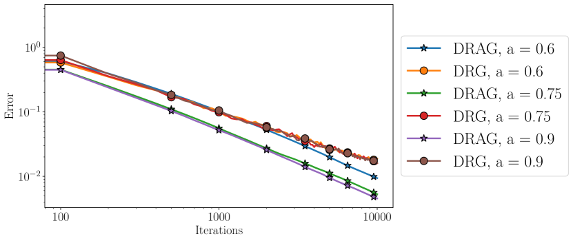
(a) Error between the estimators ${\mathbf{g}}_{t}$ and $\overline{{\mathbf{g}}}_{t}$ and the optimal potential ${\mathbf{g}}^{*}$ on Example 2, $a\in\{0,6,0.75,0.9\}$ and $\gamma_{1}=\sqrt{w_{\min}},b=0.75$.

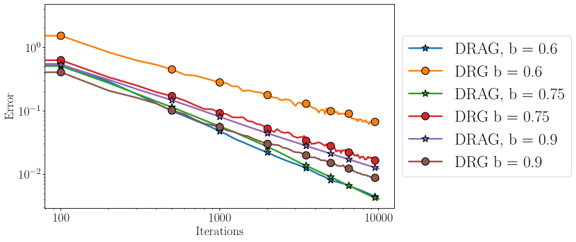
(b) Error between the estimators ${\mathbf{g}}_{t}$ and $\overline{{\mathbf{g}}}_{t}$ and the optimal potential ${\mathbf{g}}^{*}$ on Example 2, $b\in\{0,6,0.75,0.9\}$ and $\gamma_{1}=\sqrt{w_{\min}},a=0.75$.

Figure 7: Evolution of the errors, when changing one of the parameters $a$ or $b$.

As we can see, the choice $a=b=0.75$ seems to be a good compromise on this experiments. We also see on Figure 7(b) that the non-averaged estimates with the best convergence rate is when $b=0.9$. This behabiour is concordant with our theory. However, as we can see, the parameter $b=0.9$ does not yet benefits from the acceleration thanks to averaging.

DRAG compared with SGD and ASGD.

We compare here the performance of our algorithm DRAG compared to the vanilla SGD and ASGD, introduced in Genevay et al. [2016] for EOT, on Example 2. For our comparison, since we fixed the parameters of DRAG to $(\sqrt{M},3/4,3/4)$ and ran the algorithm for $t=10^{5}$ iterations, we have $\varepsilon_{t}=10^{-15/4}\simeq 10^{-4}$. We thus set $\varepsilon=\varepsilon_{t}$ to run SGD and ASGD. As we can see in Figure 8, DRAG clearly outperforms SGD and ASGD. We note that the poor convergence of SGD and ASGD is not surprising with a small regularization parameter, as already observed, for instance, in Seguy et al. [2017].

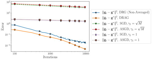
Figure 8: Comparison of DRAG with SGD and ASGD with a fixed regularization of $\varepsilon_{t}=10^{-15/4}$, on Example 2.

Appendix B Proofs of the main paper

Additionnal notations for the proofs.

For any $c>0$ we define the function $t\mapsto\Psi_{c}(t)$ such that

$$\sum_{t=1}^{T}t^{-c}\leq\Psi_{c}(T):=\left\{\begin{array}[]{lr}1+\ln(T+1)&\text{if }c=1,\\ \frac{2c-1}{c-1}&\text{if }c>1,\\ 1+\frac{1}{1-c}(T+1)^{1-c}&\text{if }c<1.\end{array}\right.$$ (16)

For a sequence $(u_{t})_{t\in\mathbb{N}}$, if $\frac{t}{2}\notin\mathbb{N}$, $u_{\frac{t}{2}}$ must be understood as $u_{\left\lceil\frac{t}{2}\right\rceil}$.

B.1 Proof of Theorem 1: Convergence rate of the non averaged iterates.

In all the sequel, we note

$$\Delta_{t} =\|{\mathbf{g}}_{t}-{\mathbf{g}}^{*}_{\varepsilon_{t}}\|^{2}.$$

Remark that the dependence in $t$ is both in the estimator ${\mathbf{g}}_{t}$ and the optimizer ${\mathbf{g}}_{\varepsilon_{t}}^{*}$. We also recall that we note $D_{\mathcal{C}}:=\underset{{\mathbf{g}},{\mathbf{g}}^{\prime}\in\cal C}{\sup}\|{\mathbf{g}}-{\mathbf{g}}^{\prime}\|<\infty$ .

We will divide the proof into two parts.

B.1.1 Part 1: proof for $p=1$.

Proof.

By definition of the gradient step at time $t+1$ and since ${\mathbf{g}}_{\varepsilon_{t+1}}^{*}\in\mathcal{C}$, we have

$$\Delta_{t+1} =\|{\mathbf{g}}_{t+1}-{\mathbf{g}}_{\varepsilon_{t+1}}^{*}\|^{2}$$

$$=\|{\mathrm{Proj}}_{{\mathcal{C}}}({\mathbf{g}}_{t}-\gamma_{t+1}\nabla_{{\mathbf{g}}}h_{\varepsilon_{t}}({\mathbf{g}}_{t},X_{t+1}))-{\mathbf{g}}_{\varepsilon_{t+1}}^{*}\|^{2}$$

$$\leq\|{\mathbf{g}}_{t}-\gamma_{t+1}\nabla_{{\mathbf{g}}}h_{\varepsilon_{t}}({\mathbf{g}}_{t},X_{t+1})-{\mathbf{g}}_{\varepsilon_{t+1}}^{*}\|^{2}.$$

Then, incorporating the change of optimum between time $t$ and $t+1$, we get

$$\Delta_{t+1} \leq\|{\mathbf{g}}_{t}-\gamma_{t+1}\nabla_{{\mathbf{g}}}h_{\varepsilon_{t}}({\mathbf{g}}_{t},X_{t+1})-{\mathbf{g}}_{\varepsilon_{t}}^{*}+{\mathbf{g}}_{\varepsilon_{t}}^{*}-{\mathbf{g}}_{\varepsilon_{t+1}}^{*}\|^{2}$$

$$\leq\|{\mathbf{g}}_{t}-\gamma_{t+1}\nabla_{{\mathbf{g}}}h_{\varepsilon_{t}}({\mathbf{g}}_{t},X_{t+1})-{\mathbf{g}}_{\varepsilon_{t}}^{*}\|^{2}+2\left\langle{\mathbf{g}}_{t}-\gamma_{t+1}\nabla_{{\mathbf{g}}}h_{\varepsilon_{t}}({\mathbf{g}}_{t},X_{t+1})-{\mathbf{g}}_{\varepsilon_{t}}^{*},{\mathbf{g}}_{\varepsilon_{t}}^{*}-{\mathbf{g}}_{\varepsilon_{t+1}}^{*}\right\rangle$$

$$\quad+\|{\mathbf{g}}_{\varepsilon_{t}}^{*}-{\mathbf{g}}_{\varepsilon_{t+1}}^{*}\|^{2}.$$

Using Corollary 2.2 in [Delalande, 2022], see (5), there exists $K_{0}>0$ such that for any $\alpha^{\prime}\in]0,\alpha[$

$$\displaystyle\|{\mathbf{g}}_{\varepsilon_{t}}^{*}-{\mathbf{g}}_{\varepsilon_{t+1}}^{*}\| \leq K_{0}\varepsilon_{t}^{\alpha^{\prime}}(\varepsilon_{t}-\varepsilon_{t+1})\leq K_{0}t^{-a\alpha^{\prime}}\left(t^{-a}-(t+1)^{-a}\right)\leq aK_{0}t^{-(1+a+a\alpha^{\prime})}.$$ (17)

For clarity, we define $r_{t}:=aK_{0}t^{-(1+a+a\alpha^{\prime})}$ and $R_{t}:=(2D_{\mathcal{C}}+2\gamma_{t+1}+r_{t})r_{t}$.

Using that for all $t$, ${\mathbf{g}}_{t}\in{\mathcal{C}}$, and that for all $x\in\mathbb{R}^{d},{\mathbf{g}}\in\mathbb{R}^{M}$, $\|\nabla_{{\mathbf{g}}}h_{\varepsilon_{t}}({\mathbf{g}},x)\|\leq 2$, we obtain

$$\Delta_{t+1} \leq\|{\mathbf{g}}_{t}-\gamma_{t+1}\nabla_{{\mathbf{g}}}h_{\varepsilon_{t}}({\mathbf{g}}_{t},X_{t+1})-{\mathbf{g}}_{\varepsilon_{t}}^{*}\|^{2}+(2D_{\mathcal{C}}+2\gamma_{t+1})\|{\mathbf{g}}_{\varepsilon_{t}}^{*}-{\mathbf{g}}_{\varepsilon_{t+1}}^{*}\|+\|{\mathbf{g}}_{\varepsilon_{t}}^{*}-{\mathbf{g}}_{\varepsilon_{t+1}}^{*}\|^{2}$$

$$\leq\|{\mathbf{g}}_{t}-\gamma_{t+1}\nabla_{{\mathbf{g}}}h_{\varepsilon_{t}}({\mathbf{g}}_{t},X_{t+1})-{\mathbf{g}}_{\varepsilon_{t}}^{*}\|^{2}+R_{t}$$

$$\leq\|{\mathbf{g}}_{t}-{\mathbf{g}}_{\varepsilon_{t}}^{*}\|^{2}-2\gamma_{t+1}\left\langle\nabla_{{\mathbf{g}}}h_{\varepsilon_{t}}({\mathbf{g}}_{t},X_{t+1}),{\mathbf{g}}_{t}-{\mathbf{g}}_{\varepsilon_{t}}^{*}\right\rangle+\gamma_{t+1}^{2}\|\nabla_{{\mathbf{g}}}h_{\varepsilon_{t}}({\mathbf{g}}_{t},X_{t+1})\|^{2}+R_{t}$$

$$\leq\Delta_{t}-2\gamma_{t+1}\left\langle\nabla_{{\mathbf{g}}}h_{\varepsilon_{t}}({\mathbf{g}}_{t},X_{t+1}),{\mathbf{g}}_{t}-{\mathbf{g}}_{\varepsilon_{t}}^{*}\right\rangle+4\gamma_{t+1}^{2}+R_{t}.$$

Note that, since we have $1+a+a\alpha>2b$, we can also take $\alpha^{\prime}\in]0,\alpha[$ such that $1+a+a\alpha^{\prime}>2b$. Therefore, the sequence $R_{t}/\gamma_{t}^{2}$ is decreasing and tends to 0. For conciseness, we note

$$t_{a,\alpha}:=\min\left\{t\geq 1:\,R_{t}\leq\gamma_{t}^{2}\right\}.$$ (18)

For any $t\geq t_{a,\alpha}$, we then obtain the following upper bound of $\Delta_{t+1}$ in terms of $\Delta_{t}$ and the gradient direction:

$$\Delta_{t+1}\leq\Delta_{t}-2\gamma_{t+1}\left\langle\nabla_{{\mathbf{g}}}h_{\varepsilon_{t}}({\mathbf{g}}_{t},X_{t+1}),{\mathbf{g}}_{t}-{\mathbf{g}}_{\varepsilon_{t}}^{*}\right\rangle+5\gamma_{t+1}^{2}.$$ (19)

Noting $\mathcal{F}_{t}$ the filtration generated by the samples $X_{1},\ldots,X_{t}\overset{\text{iid}}{\sim}\mu$, that is $\mathcal{F}_{t}=\sigma\left(X_{1},\ldots,X_{t}\right)$ and taking the conditional expectation, we have

$$\mathbb{E}\left[\Delta_{t+1}|\mathcal{F}_{t}\right]\leq\Delta_{t}-2\gamma_{t+1}\left\langle\nabla H_{\varepsilon_{t}}({\mathbf{g}}_{t}),{\mathbf{g}}_{t}-{\mathbf{g}}_{\varepsilon_{t}}^{*}\right\rangle+5\gamma_{t}^{2}.$$ (20)

Using Lemma 2 and denoting $A_{{\mathbf{g}}_{t},\varepsilon_{t}}=1-e^{-\frac{2}{\varepsilon_{t}}\left[1\wedge\|{\mathbf{g}}_{t}-{\mathbf{g}}_{\varepsilon_{t}}^{*}\|\right]}$, one has for all $t$

$$\left\langle\nabla H_{\varepsilon_{t}}({\mathbf{g}}_{t}),{\mathbf{g}}_{t}-{\mathbf{g}}_{\varepsilon_{t}}^{*}\right\rangle\geq\frac{A_{{\mathbf{g}}_{t},\varepsilon_{t}}}{K_{\mathbf{w}}}\left\|{\mathbf{g}}_{t}-{\mathbf{g}}_{t}^{*}\right\|_{2}^{2}=:\lambda_{t}\Delta_{t}.$$ (21)

Then, it comes

$$\mathbb{E}\left[\Delta_{t+1}\mid\mathcal{F}_{t}\right]\leq\left(1-2\lambda_{t}\gamma_{t+1}\right)\Delta_{t}+5\gamma_{t+1}^{2}.$$ (22)

We note

$$\lambda=\frac{w_{\min}(1-e^{-2})}{2\max\{2R^{2},1\}},$$ (23)

and note that $\lambda_{t}\geq\lambda$ if $\|{\mathbf{g}}_{t}-{\mathbf{g}}_{\varepsilon_{t}}^{*}\|_{\infty}\geq\varepsilon_{t}$. Therefore, we have

$$\mathbb{E}\left[\Delta_{t+1}\mid\mathcal{F}_{t}\right]\leq\left(1-2\lambda\gamma_{t+1}\right)\Delta_{t}+\left[2(\lambda-\lambda_{t})\mathbf{1}_{\|{\mathbf{g}}_{t}-{\mathbf{g}}_{\varepsilon_{t}}^{*}\|_{\infty}\leq\varepsilon_{t}}\right]\gamma_{t+1}\Delta_{t}+5\gamma_{t+1}^{2}.$$

Moreover, $\|{\mathbf{g}}_{t}-{\mathbf{g}}_{\varepsilon_{t}}^{*}\|_{\infty}\leq\varepsilon_{t}$ implies that $\Delta_{t}\leq M\varepsilon_{t}^{2}$. Therefore,

$$\mathbb{E}\left[\Delta_{t+1}\mid\mathcal{F}_{t}\right] \leq\left(1-2\lambda\gamma_{t+1}\right)\Delta_{t}+\left[2(\lambda-\lambda_{t})\mathbf{1}_{\|{\mathbf{g}}_{t}-{\mathbf{g}}_{\varepsilon_{t}}^{*}\|_{\infty}\leq\varepsilon_{t}}\right]\gamma_{t+1}M\varepsilon_{t}^{2}+5\gamma_{t+1}^{2}.$$

Using that $(\lambda-\lambda_{t})\mathbf{1}_{\|{\mathbf{g}}_{t}-{\mathbf{g}}_{\varepsilon_{t}}^{*}\|_{\infty}}\leq\lambda$ and taking the expectation, we obtain

$$\mathbb{E}\left[\Delta_{t+1}\right] \leq\left(1-2\lambda\gamma_{t+1}\right)\mathbb{E}[\Delta_{t}]+2\lambda M\varepsilon_{t}^{2}\gamma_{t+1}+5\gamma_{t+1}^{2}.$$

Noting $t_{\gamma}:=\min\left\{t,2\lambda\gamma_{t+1}\leq 1\right\}$ and $t_{0}:=\max\{t_{a,\alpha},t_{\gamma}\}$ , we use Proposition 1 to obtain

$$\mathbb{E}\left[\Delta_{t}\right]\leq\exp\left(-2\lambda\sum_{i=t_{0}+1}^{t}\gamma_{i}\right)\left(D_{\mathcal{C}}^{2}+\sum_{k=t_{0}}^{t}5\gamma_{k}^{2}\right)+\frac{5}{2\lambda}\gamma_{\frac{t}{2}-1}+M\varepsilon_{\frac{t}{2}-1}^{2}.$$ (24)

Applying Corollary 2, the exponential product converges exponentially to $0$. Therefore, using the value of $\lambda$ defined in (23) , an asymptotic comparison gives

$$\mathbb{E}[\Delta_{t}]\leq\frac{5[2R^{2}\vee 1]}{w_{\min}(1-e^{-2})}\gamma_{\frac{t}{2}-1}+M\varepsilon_{\frac{t}{2}-1}^{2}+\mathcal{O}(\gamma_{t}^{2})\,.$$

In the usual case where the discrete measure $\nu$ has uniform weights equal to $\frac{1}{M}$, we deduce from the relation $2a\geq b$, by the assumption of the theorem, that

$$\mathbb{E}[\Delta_{t}]=\mathcal{O}\left(M\gamma_{t}\right).$$

∎

B.1.2 Part 2: proof for $p=2$.

Proof.

Building on the proof of the case $p=1$, we start by squaring equation (19). For $t\geq t_{a,\alpha}$, where $t_{a,\alpha}$ is defined in (18), we have

$$\Delta_{t+1}^{2} \leq\left(\Delta_{t}-2\gamma_{t+1}\left\langle\nabla_{{\mathbf{g}}}h_{\varepsilon_{t}}({\mathbf{g}}_{t},X_{t+1}),{\mathbf{g}}_{t}-{\mathbf{g}}_{\varepsilon_{t}}^{*}\right\rangle+5\gamma_{t+1}^{2}\right)^{2}$$

$$\leq\Delta_{t}^{2}+4\gamma_{t+1}^{2}\left\langle\nabla_{{\mathbf{g}}}h_{\varepsilon_{t}}({\mathbf{g}}_{t},X_{t+1}),{\mathbf{g}}_{t}-{\mathbf{g}}_{\varepsilon_{t}}^{*}\right\rangle^{2}+25\gamma_{t+1}^{4}$$

$$\quad-\underbrace{2\Delta_{t}\gamma_{t+1}\left\langle\nabla_{{\mathbf{g}}}h_{\varepsilon_{t}}({\mathbf{g}}_{t},X_{t+1}),{\mathbf{g}}_{t}-{\mathbf{g}}_{\varepsilon_{t}}^{*}\right\rangle}_{=:A}+5\Delta_{t}\gamma_{t+1}^{2}-\underbrace{10\gamma_{t+1}^{3}\left\langle\nabla_{{\mathbf{g}}}h_{\varepsilon_{t}}({\mathbf{g}}_{t},X_{t+1}),{\mathbf{g}}_{t}-{\mathbf{g}}_{\varepsilon_{t}}^{*}\right\rangle}_{=:B}.$$

Taking the conditional expectation, recalling that $\lambda_{t}$ is defined in 21, we obtain thanks to Lemma 2

$$\mathbb{E}[A\mid\mathcal{F}_{t}]\geq 2\Delta_{t}^{2}\lambda_{t}\gamma_{t+1}.$$

We also use the simple bound

$$\mathbb{E}[B\mid\mathcal{F}_{t}]\geq 0.$$

These two inequalities lead to

$$\mathbb{E}[\Delta_{t}^{2}\mid\mathcal{F}_{t}]\leq\Delta_{t}^{2}(1-2\lambda_{t}\gamma_{t+1})+4\gamma_{t+1}^{2}\mathbb{E}\left[\left\langle\nabla h_{\varepsilon_{t}}\left({\mathbf{g}}_{t},X_{t+1}\right),{\mathbf{g}}_{t}-{\mathbf{g}}_{\varepsilon_{t}}^{*}\right\rangle^{2}\mid\mathcal{F}_{t}\right]+25\gamma_{t+1}^{4}+5\Delta_{t}\gamma_{t+1}^{2}.$$ (25)

Using that the gradient norm is bounded by two, we use Cauchy-Schwarz inequality to obtain

$$4\gamma_{t+1}^{2}\left\langle\nabla_{{\mathbf{g}}}h_{\varepsilon_{t}}({\mathbf{g}}_{t},X_{t+1}),{\mathbf{g}}_{t}-{\mathbf{g}}_{\varepsilon_{t}}^{*}\right\rangle^{2} \leq 16\gamma_{t+1}^{2}\|{\mathbf{g}}_{t}-{\mathbf{g}}_{\varepsilon_{t}}^{*}\|^{2}\leq 16\Delta_{t}\gamma_{t+1}^{2}.$$

Recalling the value of $\lambda$ defined in (23):

$$\lambda=\frac{w_{\min}(1-e^{-2})}{2\max\{2R^{2},1\}},$$

we use Hölder’s inequality to obtain

$$21\Delta_{t}\gamma_{t+1}^{2} \leq\left(\Delta_{t}\sqrt{2\lambda}\frac{1}{\sqrt{2\lambda}}21\gamma_{t+1}\right)\gamma_{t+1}$$

$$\leq\gamma_{t+1}\Delta_{t}^{2}\lambda+\frac{21^{2}}{4\lambda}\gamma_{t+1}^{3}.$$

Summing up these inequalities, we obtain

$$\mathbb{E}[\Delta_{t+1}^{2}\mid\mathcal{F}_{t}] \leq(1-2\lambda_{t}\gamma_{t+1}+\lambda\gamma_{t+1})\Delta_{t}^{2}+\frac{21^{2}}{4\lambda}\gamma_{t+1}^{3}+25\gamma_{t+1}^{4}.$$

Similarly to the case $p=1$, we have

$$\mathbb{E}[\Delta_{t+1}^{2}\mid\mathcal{F}_{t}] \leq(1-2\lambda\gamma_{t+1}+\lambda\gamma_{t+1})\Delta_{t}^{2}+\left[2(\lambda-\lambda_{t})\mathbf{1}_{\|{\mathbf{g}}_{t}-{\mathbf{g}}_{\varepsilon_{t}}^{*}\|_{\infty}\leq\varepsilon_{t}}\right]\Delta_{t}^{2}\gamma_{t+1}+\frac{21^{2}}{4\lambda}\gamma_{t+1}^{3}+25\gamma_{t+1}^{4}$$

$$\leq(1-\lambda\gamma_{t+1})\Delta_{t}^{2}+2\lambda M^{2}\varepsilon_{t}^{4}\gamma_{t+1}+\frac{21^{2}}{4\lambda}\gamma_{t+1}^{3}+25\gamma_{t+1}^{4}.$$

Taking the expectation, we obtain

$$\mathbb{E}[\Delta_{t+1}^{2}] \leq(1-\lambda\gamma_{t+1})\mathbb{E}[\Delta_{t}^{2}]+2\lambda M^{2}\varepsilon_{t}^{4}\gamma_{t+1}+\frac{21^{2}}{4\lambda}\gamma_{t+1}^{3}+25\gamma_{t+1}^{4}.$$

Proceeding as for the case $p=1$, that is, applying Proposition 1 and Corollary 2 concludes the proof.

∎

B.2 Proof of Theorem 2: Convergence rate of DRPASGD

Proof.

We start by a decomposition of the gradient step, already present in Godichon and Portier [2017]. By abuse of notation, we note

$$\nabla_{k}^{2}:=\nabla^{2}H_{\varepsilon_{k}}({\mathbf{g}}_{\varepsilon_{k}}^{*})$$

and define the following differences:

$$p_{k} :=\mathrm{Proj}_{{\mathcal{C}}}\left({\mathbf{g}}_{k}-\gamma_{k+1}\nabla_{{\mathbf{g}}}h_{\varepsilon_{k}}\left({\mathbf{g}}_{k},X_{k+1}\right)\right)-\left({\mathbf{g}}_{k}-\gamma_{k+1}\nabla_{{\mathbf{g}}}h_{\varepsilon_{k}}\left({\mathbf{g}}_{k},X_{k+1}\right)\right),$$

$$\xi_{k+1} :=\nabla H_{\varepsilon_{k}}\left({\mathbf{g}}_{k}\right)-\nabla_{{\mathbf{g}}}h_{\varepsilon_{k}}\left({\mathbf{g}}_{k},X_{k+1}\right),$$

$$\delta_{k} :=\nabla H_{\varepsilon_{k}}\left({\mathbf{g}}_{k}\right)-\nabla_{k}^{2}\left({\mathbf{g}}_{k}-{\mathbf{g}}_{k}^{*}\right).$$

The term $p_{k}$ represents the difference between the projected and non-projected steps. Remark that $p_{k}=0$ if ${\mathbf{g}}_{k}-\gamma_{k+1}\nabla_{{\mathbf{g}}}h_{\varepsilon_{k}}\left({\mathbf{g}}_{k},X_{k+1}\right)\in{\mathcal{C}}$. The difference of martingale $\xi_{k}$ represents the difference between the gradient and its unbiased version. Finally, $\delta_{k}$ represents the difference between the gradient at ${\mathbf{g}}_{k}$ with the linearized Hessian at the optimum.

Noting $I_{M}$ the identity matrix of $\mathcal{M}_{M}(\mathbb{R})$, observe that for any $k\in\mathbb{N}$

$${\mathbf{g}}_{k+1}-{\mathbf{g}}_{\varepsilon_{k}}^{*} =\mathrm{Proj}_{{\mathcal{C}}}\left({\mathbf{g}}_{k}-\gamma_{k+1}\nabla_{{\mathbf{g}}}h_{\varepsilon_{k}}({\mathbf{g}}_{k},X_{k+1})\right)-{\mathbf{g}}_{\varepsilon_{k}}^{*}$$

$$={\mathbf{g}}_{k}-\gamma_{k+1}\nabla_{{\mathbf{g}}}h_{\varepsilon_{k}}({\mathbf{g}}_{k},X_{k+1})-{\mathbf{g}}_{\varepsilon_{k}}^{*}-p_{k}$$

$$={\mathbf{g}}_{k}-\gamma_{k+1}\nabla H_{\varepsilon_{k}}({\mathbf{g}}_{k},X_{k+1})-{\mathbf{g}}_{\varepsilon_{k}}^{*}+\gamma_{k+1}\xi_{k+1}-p_{k}$$

$$=\left(I_{M}-\gamma_{k+1}\nabla^{2}_{k}\right)\left({\mathbf{g}}_{k}-{\mathbf{g}}_{k}^{*}\right)-\gamma_{k+1}\delta_{k}+\gamma_{k+1}\xi_{k+1}+p_{k}.$$

Thus, we have that

$$\nabla_{k}^{2}\left({\mathbf{g}}_{k}-{\mathbf{g}}_{\varepsilon_{k}}^{*}\right)=\frac{{\mathbf{g}}_{k}-{\mathbf{g}}_{k+1}}{\gamma_{k+1}}-\delta_{k}+\xi_{k+1}+\frac{p_{k}}{\gamma_{k}}.$$

Observe that there is an orthogonal matrix $U_{k}$ such that $\nabla_{k}^{2}=U_{k}\,\text{diag}\left(\lambda_{k,1},\ldots,\lambda_{k,M-1},0\right)U_{k}^{\top}$. Therefore, in the following, we denote

$$\left(\nabla_{k}^{2}\right)^{-1}=U_{k}\,\text{diag}\left(\lambda_{k,1}^{-1},\ldots,\lambda_{k,M-1}^{-1},0\right)U_{k}^{\top}$$

the inverse of $\nabla_{k}^{2}$ in the space $\mathrm{Vect}(\mathbf{1}_{M})^{\bot}$. Note that we have (Bercu and Bigot [2021], Lemma A.1, equation (A.4))

$$\min_{j\in\llbracket 1,M-1\rrbracket}\lambda_{k,j}\geq\frac{w_{\min}}{\varepsilon_{k}}\,,\qquad k\geq 0.$$

Taking all the equalities in $\mathrm{Vect}(\mathbf{1}_{M})^{\bot}$, that is, considering all our vectors in the subspace $\mathrm{Vect}(\mathbf{1}_{M})^{\bot}$, we have

$$\left(\overline{{\mathbf{g}}}_{t}-{\mathbf{g}}_{\varepsilon_{t}}^{*}\right) =\frac{1}{t+1}\underbrace{\sum_{k=0}^{t}\left(\nabla_{k}^{2}\right)^{-1}\frac{{\mathbf{g}}_{k}-{\mathbf{g}}_{k+1}}{\gamma_{k+1}}}_{:=L_{1,t}}-\frac{1}{t+1}\underbrace{\sum_{k=0}^{t}\left(\nabla_{k}^{2}\right)^{-1}\delta_{k}}_{:=L_{2,t}}$$

$$+\frac{1}{t+1}\underbrace{\sum_{k=0}^{t}\left(\nabla_{k}^{2}\right)^{-1}\xi_{k+1}}_{:=M_{t}}+\frac{1}{t+1}\underbrace{\sum_{k=0}^{t}\left(\nabla_{k}^{2}\right)^{-1}\frac{p_{k}}{\gamma_{k+1}}}_{:=L_{3,t}}+\frac{1}{t+1}\underbrace{\sum_{k=0}^{t}\left(\mathbf{g}_{k}^{*}-\mathbf{g}_{t}^{*}\right)}_{=:D_{t}}.$$

Remark that the term $\frac{1}{t+1}D_{t}$ comes from the difference between $\frac{1}{t+1}\sum_{k=0}^{t}{\mathbf{g}}_{\varepsilon_{k}}^{*}$ and ${\mathbf{g}}_{\varepsilon_{t}}^{*}$.

We will now bound the convergence rate for each of the sums in our decomposition. Note that the terms $L_{1,t},L_{2,t}$ and $L_{3,t}$ will be, surprisingly, the limiting terms. Indeed, in stochastic optimization, $M_{t}$ is usually the main term. Nevertheless, the presence of the inverse of the Hessian $\left(\nabla_{k}^{2}\right)^{-1}$, whose largest eigenvalues is of order $\varepsilon_{k}$, decreasing with $k\geq 1$, makes it negligible.

$\bullet$ Convergence rate for $L_{1,t}$. By the definition of our gradient step, we have

$$\frac{1}{t+1}L_{1,t}=\frac{1}{t+1}\sum_{k=0}^{t}\left(\nabla_{k}^{2}\right)^{-1}\frac{\gamma_{k+1}\nabla_{{\mathbf{g}}}h_{\varepsilon_{k}}({\mathbf{g}}_{k},x_{k+1})}{\gamma_{k+1}}.$$

Then, using that the gradient norm is bounded by $2$, we obtain

$$\frac{1}{t+1}\left(\mathbb{E}\left[\|L_{1,t}\|^{2}\right]\right)^{\frac{1}{2}} \leq\frac{2}{t+1}\sum_{k=0}^{t}\|(\nabla_{k}^{2})^{-1}\|$$

$$\leq\frac{2w_{\min}^{-1}}{t+1}\Psi_{a}(t).$$

$\bullet$ Convergence rate for $L_{2,t}$. Using Lemma 2, for all $k\geq 0$, we have

$$\|\delta_{k}\| =\left\|\nabla H_{\varepsilon_{k}}({\mathbf{g}}_{k})-\nabla^{2}H_{\varepsilon_{k}}\left({\mathbf{g}}_{\varepsilon_{k}}^{*}\right)\left({\mathbf{g}}_{k}-{\mathbf{g}}_{\varepsilon_{k}}^{*}\right)\right\|\leq\frac{4}{\varepsilon_{k}}\|{\mathbf{g}}_{k}-{\mathbf{g}}_{\varepsilon_{k}}^{*}\|_{\infty}^{2}.$$

In addition, thanks to Theorem 1, $\mathbb{E}\left[\Delta_{k}^{2}\right]=\mathcal{O}(w_{\min}^{-2}\gamma_{k}^{2})$. That is, there is a positive constant $C_{2}$ such that for all $k\geq 1$, we have $\mathbb{E}\left[\Delta_{k}^{2}\right]\leq C_{2}w_{\min}^{-2}k^{-2b}$. Therefore,

$$\frac{1}{t+1}\left(\mathbb{E}\left[\left\|L_{2,t}\right\|^{2}\right]\right)^{\frac{1}{2}} \leq\frac{4w_{\min}^{-1}}{(t+1)}\sum_{k=0}^{t}\sqrt{\mathbb{E}\left[\left\|{\mathbf{g}}_{k}-{\mathbf{g}}_{\varepsilon_{k}}^{*}\right\|_{\infty}^{4}\right]}$$

$$\leq\frac{4w_{\min}^{-1}}{(t+1)}\sum_{k=0}^{t}\sqrt{\mathbb{E}\left[\Delta_{k}^{2}\right]}$$

$$\leq\frac{4w_{\min}^{-2}\sqrt{C_{2}}}{(t+1)}\Psi_{b}(t)$$

$$=\mathcal{O}(w_{\min}^{-2}t^{-b})\,.$$

Remark: When the weights are uniform, i.e., $w_{\min}=1/M$, the bound can be of the order of $M$ smaller since $\|.\|_{\infty}\leq\|.\|\leq\sqrt{M-1}\|.\|_{\infty}$. Therefore, the bound can be closer to

$$\frac{1}{t+1}\left(\mathbb{E}\left[\left\|L_{2,t}\right\|^{2}\right]\right)^{\frac{1}{2}} =\mathcal{O}(Mt^{-b}).$$

To emphasis this, we can fix $\beta\in[0,1]$ such that, when $\mathbf{w}=\frac{1}{M}\mathbf{1}_{M}$, we have

$$\frac{1}{t+1}\left(\mathbb{E}\left[\left\|L_{2,t}\right\|^{2}\right]\right)^{\frac{1}{2}} =\mathcal{O}(M^{1+\beta}t^{-b}).$$

$\bullet$ Convergence rate for $L_{3,t}$. In the same way as for $L_{1,t}$, we have that for any $k$

$$\|p_{k}\|\leq 2\gamma_{k}\ ,$$

such that

$$\frac{1}{t+1}\left(\mathbb{E}\left[\|L_{3,t}\|^{2}\right]\right)^{\frac{1}{2}} \leq\sum_{k=0}^{t}2\|(\nabla_{k}^{2})^{-1}\|\leq 2w_{\min}^{-1}\Psi_{a}(t).$$

However, we can retrieve a better convergence rate for this term.

$\bullet$ Convergence rate for $M_{t}$. Observe that

$$\mathbb{E}[\|M_{t}\|^{2}]=\mathbb{E}\left[\|M_{t-1}\|^{2}+2\left\langle(\nabla_{t}^{2})^{-1\top}M_{t-1},\xi_{t}\right\rangle+\|(\nabla_{t}^{2})^{-1}\|^{2}\|\xi_{t}\|^{2}\right],$$

with

$$\mathbb{E}\left[\left\langle(\nabla_{t}^{2})^{-1\top}M_{t-1},\xi_{t}\right\rangle\right]=0.$$

Moreover, we have $\|\xi\|\leq 4$, such that

$$\frac{1}{t+1}\left(\mathbb{E}[\|M_{t}\|^{2}]\right)^{1/2} =\frac{4w_{\min}^{-1}}{t+1}\sqrt{\Psi_{2a}(t)}\leq\sqrt{\frac{2a}{2a-1}}\frac{4w_{\min}^{-1}}{t+1}.$$

$\bullet$ Convergence rate for $D_{t}$. Thanks to (5), one as for all $0<\alpha^{\prime}<\alpha$,

$$\frac{1}{t+1}D_{t} \leq\frac{K_{0}}{t+1}\sum_{k=0}^{t}\varepsilon_{k}^{\alpha^{\prime}}\left(\varepsilon_{k}-\varepsilon_{t}\right)$$

$$\leq\frac{K_{0}}{t+1}\sum_{k=0}^{t}\varepsilon_{k}^{1+\alpha^{\prime}}$$

$$\leq\frac{K_{0}}{t+1}\Psi_{a+a\alpha^{\prime}}(t),$$

and this term is negligible since $a+\alpha^{\prime}>b$.

$\bullet$ Conclusion. Taking $a\geq b$ as in the Theorem’s assumption and summing up the inequalities, we obtain

$$\mathbb{E}\left[\|\overline{{\mathbf{g}}}_{t}-{\mathbf{g}}_{\varepsilon_{t}}^{*}\|^{2}\right]^{\frac{1}{2}} \leq\mathcal{O}(w_{\min}^{2}t^{-b})+o(t^{-b}).$$

When $\mathbf{w}=\frac{1}{M}\mathbf{1}_{M}$, we obtain

$$\mathbb{E}\left[\|\overline{{\mathbf{g}}}_{t}-{\mathbf{g}}_{\varepsilon_{t}}^{*}\|^{2}\right]^{\frac{1}{2}} \leq\mathcal{O}(M^{1+\beta}t^{-b})+o(t^{-b}).$$

Using (5), for any $\alpha^{\prime}<\alpha$ we have

$$\|{\mathbf{g}}_{\varepsilon_{t}}^{*}-{\mathbf{g}}^{*}\|\leq K_{0}\varepsilon_{t}^{1+\alpha^{\prime}}\leq K_{0}t^{a+a\alpha^{\prime}}=o(t^{-b}).$$

Finally, we have

$$\mathbb{E}\left[\|\overline{{\mathbf{g}}}_{t}-{\mathbf{g}}^{*}\|^{2}\right]^{\frac{1}{2}} \leq\mathcal{O}(w_{\min}^{2}t^{-b})+o(t^{-b}),$$

and when $\mathbf{w}=\frac{1}{M}\mathbf{1}_{M}$,

$$\mathbb{E}\left[\|\overline{{\mathbf{g}}}_{t}-{\mathbf{g}}^{*}\|^{2}\right]^{\frac{1}{2}} \leq\mathcal{O}(M^{1+\beta}t^{-b})+o(t^{-b}).$$

Remark: The main theorem considers $a\geq b$ to have the best convergence rate. However, note that from the proof, we can read the result when $b/2\leq a<b$. In this case, the limiting terms are only $L_{1,t}$ and $L_{3,t}$.

∎

B.3 Proof of Corollary 1: OT cost estimation

Proof.

EOT cost estimation.

For any $\varepsilon>0$, the function $H_{\varepsilon}$ is $\frac{1}{\varepsilon}$-smooth. Therefore, for any ${\mathbf{g}}\in\mathbb{R}^{M}$, we have

$$H_{\varepsilon}({\mathbf{g}})-H_{\varepsilon}({\mathbf{g}}_{\varepsilon}^{*})\leq\frac{1}{2\varepsilon}\|{\mathbf{g}}_{\varepsilon}^{*}-{\mathbf{g}}\|^{2}.$$

Using our estimator $\overline{{\mathbf{g}}_{t}}$ and (5), we obtain

$$H_{\varepsilon}(\overline{{\mathbf{g}}}_{t})-H_{\varepsilon}({\mathbf{g}}_{\varepsilon}^{*}) \leq\frac{1}{\varepsilon}\left(\|{\mathbf{g}}_{\varepsilon}^{*}-{\mathbf{g}}_{t}^{*}\|^{2}+\|\overline{{\mathbf{g}}}_{t}-{\mathbf{g}}_{t}^{*}\|^{2}\right)$$

$$\lesssim\varepsilon^{2\alpha^{\prime}-1}(\varepsilon-\varepsilon_{t})^{2}+\frac{1}{\varepsilon t^{2b}}.$$

Remark. Using the triangular inequality and Theorem 2.3 in Delalande [2022], we also have

$$\left|H_{0}({\mathbf{g}}^{*})-H_{\varepsilon}(\overline{{\mathbf{g}}}_{t})\right|\lesssim\varepsilon^{2}+\varepsilon^{2\alpha^{\prime}-1}(\varepsilon-\varepsilon_{t})^{2}+\frac{1}{\varepsilon t^{2b}}.$$

OT cost estimation. For any vector ${\mathbf{g}}\in\mathbb{R}^{M}$, we recall the definition of $\mathbb{L}({\mathbf{g}})=\bigcup_{j=1}^{M}\mathbb{L}_{i}({\mathbf{g}})$ :

$$\text{for all }j\in\llbracket 1,M\rrbracket,\ \mathbb{L}_{j}({\mathbf{g}}):=\left\{x\in\mathbb{R}^{d};{\mathbf{g}}^{c}(x)=\frac{1}{2}\|x-y_{j}\|_{2}^{2}-g_{j}\right\}.$$

Note that $\mathbb{L}({\mathbf{g}})$ defines a partition, i.e. $\mu\left(\mathbb{L}_{i}({\mathbf{g}})\cap\mathbb{L}_{j}({\mathbf{g}})\right)=0$ when $i\neq j$, and the convex sets $\mathbb{L}_{j}({\mathbf{g}})$ are called power or Laguerre cells. We define the set

$$\mathcal{K}^{\delta}:=\left\{{\mathbf{g}}:\mathbb{R}^{M}\rightarrow\mathbb{R}\mid\forall i\in\llbracket 1,M\rrbracket,\mu\left(\mathbb{L}_{i}({\mathbf{g}})\right)>\delta\right\}.$$

Using Theorem 4.1 in Kitagawa et al. [2019], under Assumption 1, $H_{0}$ is uniformly $C^{2,\alpha}$ on $K^{\delta}$. That is, there exists a constant $L$ such that $H_{0}$ is $L$-smooth on $\mathcal{K}^{\delta}$. Note that the constant $L$ depends on $\mu_{\min}$, $\delta$, $R$. We refer to Kitagawa et al. [2019], Remark 4.1 for more details.

By the first order condition, as soon as $\delta\leq w_{\min}$, we have ${\mathbf{g}}^{*}\in\mathcal{K}^{\delta}$. Indeed, at the optimum, we have for all $i\in\llbracket 1,M\rrbracket,\mathbb{L}_{i}({\mathbf{g}}^{*})=w_{i}$. We fix here $\delta=\frac{1}{10}w_{\min}$.

Thanks to the $L$-smoothness, for any ${\mathbf{g}}\in\mathcal{K}^{\delta}$, we have

$$|H_{0}({\mathbf{g}})-H_{0}({\mathbf{g}}^{*})|\leq\frac{L}{2}\|{\mathbf{g}}-{\mathbf{g}}^{*}\|^{2}.$$

Note that, for any ${\mathbf{g}}\in\mathbb{R}^{M}$ and $i\in\llbracket 1,M\rrbracket$, the difference of measure of the Laguerre cells $\mathbb{L}_{i}({\mathbf{g}})$ and $\mathbb{L}_{i}({\mathbf{g}}^{*})$ is at most linear with respect to $\|{\mathbf{g}}-{\mathbf{g}}^{*}\|_{\infty}$. We refer to Theorem 4 or Section 6.4.2 in Santambrogio [2015] for more details.

Therefore, there exists a constant $C_{L}$ such that, as soon as $\|{\mathbf{g}}-{\mathbf{g}}^{*}\|^{2}\leq C_{L}$, we have that ${\mathbf{g}}\in K^{\delta}$. This constant depends on $\delta,\mu_{\max}$, $R$ and $d$ as in Theorem 4. Using Theorem 2, $\mathbb{E}[\|\overline{{\mathbf{g}}}_{t}-{\mathbf{g}}^{*}\|^{2}]=\mathcal{O}(t^{-2b})$. Then

$$\mathbb{E}\left[|H_{0}(\overline{{\mathbf{g}}}_{t})-H_{0}({\mathbf{g}}^{*})|\right] =\mathbb{E}\left[|H_{0}(\overline{{\mathbf{g}}}_{t})-H_{0}({\mathbf{g}}^{*})|\mathbf{1}_{\overline{{\mathbf{g}}}_{t}\in K^{\delta}}\right]+\mathbb{E}\left[|H_{0}(\overline{{\mathbf{g}}}_{t})-H_{0}({\mathbf{g}}^{*})|\mathbf{1}_{\overline{{\mathbf{g}}}_{t}\notin K^{\delta}}\right]$$

$$\leq\frac{L}{2}\mathbb{E}[\|\overline{{\mathbf{g}}}_{t}-{\mathbf{g}}^{*}\|^{2}]+\max_{{\mathbf{g}}\in{\mathcal{C}}}|H_{0}({\mathbf{g}})-H_{0}({\mathbf{g}}^{*})|\mathbb{E}[\mathbf{1}_{\overline{{\mathbf{g}}}_{t}\notin K^{\delta}}]$$

$$\leq\frac{L}{2}\mathbb{E}[\|\overline{{\mathbf{g}}}_{t}-{\mathbf{g}}^{*}\|^{2}]+\max_{{\mathbf{g}}\in{\mathcal{C}}}|H_{0}({\mathbf{g}})-H_{0}({\mathbf{g}}^{*})|\mathbb{E}[\mathbf{1}_{\|\overline{{\mathbf{g}}}_{t}-{\mathbf{g}}^{*}\|^{2}>C_{L}}]$$

$$=\mathcal{O}(t^{-2b})\,,$$

where the Markov inequality of order 1 was used on $\mathbb{E}[\mathbf{1}_{\|\overline{{\mathbf{g}}}_{t}-{\mathbf{g}}^{*}\|^{2}>C_{L}}]$. ∎

B.4 Proof of Theorem 4: OT map estimation

Proof.

We will show here that a rate of convergence of $\overline{{\mathbf{g}}}_{t}$ to ${\mathbf{g}}_{0}^{*}$ gives a convergence rate for the map estimation. The Brenier map is equal to $T_{\mu,\nu}(x)=x-\nabla({\mathbf{g}}_{0}^{*})^{c}(x)$; see for instance Santambrogio [2015], Theorem 1.17. We will thus focus on the convergence of $\nabla\overline{{\mathbf{g}}}_{t}^{c}$ to $\nabla({\mathbf{g}}_{0}^{*})^{c}$.

For all $j\in\llbracket 1,M\rrbracket$, if $x$ is the interior of $\mathbb{L}_{j}({\mathbf{g}})$, we have

$$\nabla{\mathbf{g}}^{c}(x)=x-y_{j}.$$ (26)

Therefore, given ${\mathbf{g}},{\mathbf{g}}^{\prime}\in\mathbb{R}^{M}$, if there exists a $j\in\llbracket 1,M\rrbracket$ such that $x$ is the interior of $\mathbb{L}_{j}({\mathbf{g}})\cap\mathbb{L}_{j}({\mathbf{g}}^{\prime})$ we have

$$\nabla{\mathbf{g}}^{c}(x)=\nabla({\mathbf{g}}^{\prime})^{c}(x).$$

We will now follow arguments from Santambrogio [2015], Section 6.4.2. Fix $j,j^{\prime}\in\llbracket 1,M\rrbracket$ such that $j\neq j^{\prime}$ and $x$ is in the interior of $\mathbb{L}_{j}({\mathbf{g}})\cap\mathbb{L}_{j^{\prime}}({\mathbf{g}}^{\prime})$. By definition of the $c$-transform, we can see that $\mathbb{L}_{j}({\mathbf{g}})$ is defined by $M-1$ linear inequalities of the form

$$\langle x,y_{j^{\prime}}-y_{j}\rangle\leq a_{{\mathbf{g}}}(j,j^{\prime}):=g_{j}-g_{j^{\prime}}+\frac{1}{2}\|y_{j^{\prime}}\|_{2}^{2}-\frac{1}{2}\|y_{j}\|_{2}^{2}\,.$$

Similarly, interchanging the role of ${\mathbf{g}}$, ${\mathbf{g}}^{\prime}$ and $j$, $j^{\prime}$ we have

$$\langle x,y_{j}-y_{j^{\prime}}\rangle\leq a_{{\mathbf{g}}^{\prime}}(j^{\prime},j):=g_{j^{\prime}}^{\prime}-g_{j}^{\prime}+\frac{1}{2}\|y_{j}\|_{2}^{2}-\frac{1}{2}\|y_{j^{\prime}}\|_{2}^{2}\,.$$

We obtain that

$$\mathbb{L}_{j}({\mathbf{g}})\cap\mathbb{L}_{j^{\prime}}({\mathbf{g}}^{\prime})\subset\{x\in\mathbb{R}^{d}:-a_{{\mathbf{g}}^{\prime}}(j^{\prime},j)\leq\langle x,y_{j^{\prime}}-y_{j}\rangle\leq a_{{\mathbf{g}}}(j,j^{\prime})\}\,.$$

Moreover, noting $h=(h_{1},...,h_{M})={\mathbf{g}}-{\mathbf{g}}^{\prime}$, we see that

$$\left|a_{{\mathbf{g}}^{\prime}}(j^{\prime},j)+a_{{\mathbf{g}}}(j,j^{\prime})\right|\leq|h_{j^{\prime}}-h_{j}|\,.$$ (27)

We have

$$\mu\left(\mathcal{A}:=\left\{x\in\mathbb{R}^{d},\nabla{\mathbf{g}}^{c}(x)\neq\nabla({\mathbf{g}}^{\prime})^{c}(x)\right\}\right)$$

$$=\mu\left(\bigcup_{j<j^{\prime}}\mathbb{L}_{j}({\mathbf{g}})\cap\mathbb{L}_{j^{\prime}}({\mathbf{g}}^{\prime})\right)$$

$$\leq\sum_{j<j^{\prime}}\mu\left(\mathbb{L}_{j}({\mathbf{g}})\cap\mathbb{L}_{j^{\prime}}({\mathbf{g}}^{\prime})\right)$$

$$\leq\sum_{j<j^{\prime}}\mu\left(\{x\in\mathbb{R}^{d}:-a_{{\mathbf{g}}^{\prime}}(j^{\prime},j)\leq\langle x,y_{j^{\prime}}-y_{j}\rangle\leq a_{{\mathbf{g}}}(j,j^{\prime})\}\right)\,.$$

Under Assumption 1 $\mu$ is a measure such that $\mathrm{Supp}(\mu)\subset B(0,R)$ and it admits a density $\mathrm{d}\mu$ bounded by $\mathrm{d}\mu_{\max}$. Thus

$$\mu(\mathcal{A}) \leq\mathrm{d}\mu_{\max}\sum_{j<j^{\prime}}\mathbb{\lambda}_{\mathbb{R}^{d}}(\{x\in B(0,R):-a_{{\mathbf{g}}^{\prime}}(j^{\prime},j)\leq\langle x,y_{j^{\prime}}-y_{j}\rangle\leq a_{{\mathbf{g}}}(j,j^{\prime})\})$$

$$\leq\mathrm{d}\mu_{\max}\sum_{j<j^{\prime}}\mathbb{\lambda}_{\mathbb{R}^{d}}\left(\left\{x\in B(0,R):-\dfrac{a_{{\mathbf{g}}^{\prime}}(j^{\prime},j)}{\|y_{j^{\prime}}-y_{j}\|_{2}}\leq\left\langle x,\dfrac{y_{j^{\prime}}-y_{j}}{\|y_{j^{\prime}}-y_{j}\|_{2}}\right\rangle\leq\dfrac{a_{{\mathbf{g}}}(j,j^{\prime})}{\|y_{j^{\prime}}-y_{j}\|_{2}}\right\}\right)$$

$$\leq\mathrm{d}\mu_{\max}\sum_{j<j^{\prime}}\lambda_{\mathbb{R}^{d}}\left(\left\{x\in B(0,R):-\dfrac{a_{{\mathbf{g}}^{\prime}}(j^{\prime},j)}{\|y_{j^{\prime}}-y_{j}\|_{2}}\leq x_{1}\leq\dfrac{a_{{\mathbf{g}}}(j,j^{\prime})}{\|y_{j^{\prime}}-y_{j}\|_{2}}\right\}\right)\,.$$

by isotropy of the Lebesgue measure. Combining this remark with (27) yields

$$\mu(\mathcal{A})\leq\mathrm{d}\mu_{\max}R^{d-1}\sum_{j<j^{\prime}}\dfrac{|h_{j^{\prime}}-h_{j}|}{\|y_{j^{\prime}}-y_{j}\|_{2}}\,.$$

Similarly

$$\|\|\left(\nabla{\mathbf{g}}^{c}(\cdot)-\nabla({\mathbf{g}}^{\prime})^{c}(\cdot)\right\|_{q}\|_{L^{p}(\mu)}^{p} \leq\sum_{j<j^{\prime}}\int_{\mathbb{L}_{j}({\mathbf{g}})\cap\mathbb{L}_{j^{\prime}}({\mathbf{g}}^{\prime})}\|\left(\nabla{\mathbf{g}}^{c}(\cdot)-\nabla({\mathbf{g}}^{\prime})^{c}(\cdot)\right\|_{q}d\mu(x)$$

$$\leq\sum_{j<j^{\prime}}\|y_{j^{\prime}}-y_{j}\|_{q}\mu\left(\mathbb{L}_{j}({\mathbf{g}})\cap\mathbb{L}_{j^{\prime}}({\mathbf{g}}^{\prime})\right)$$

$$\leq\mathrm{d}\mu_{\max}R^{d-1}\sum_{j<j^{\prime}}\dfrac{\|y_{j^{\prime}}-y_{j}\|_{q}|h_{j^{\prime}}-h_{j}|}{\|y_{j^{\prime}}-y_{j}\|_{2}}$$

$$\leq\mathrm{d}\mu_{\max}M^{(2-q)_{+}/2q}R^{d-1}2M\|h\|_{1}\,.$$

So, in particular, there exists $C_{\Delta}>0$ independent of the location of the points $y_{j}$ but growing at least linearly in $M$ such that

$$\|\|\left(\nabla{\mathbf{g}}^{c}(\cdot)-\nabla({\mathbf{g}}^{\prime})^{c}(\cdot)\right\|_{q}\|_{L^{p}(\mu)}^{p} \leq C_{\Delta}\|{\mathbf{g}}-{\mathbf{g}}^{\prime}\|_{1}\leq C_{\Delta}\sqrt{M}\|{\mathbf{g}}-{\mathbf{g}}^{\prime}\|.$$

Plugging the convergence rate of $\overline{{\mathbf{g}}}_{t}$ to ${\mathbf{g}}^{*}$ concludes the proof. ∎

B.5 Proof of Theorem 3: Minimax estimation of the discrete OT potential

Proof.

Let $\Theta\subseteq\left\{\theta=(\theta_{1},...,\theta_{M})\in\mathbb{R}^{M};\theta_{1}=0\right\}$ and $\nu$ be a fixed discrete measure. For each $\theta\in\Theta$, consider $\rho_{\theta}\in{\mathcal{P}}_{\alpha}(B(0,R))$ such that $\theta$ is the only vector in $\Theta$ for which the couple $(\theta^{c},\theta)$ is solution of the dual of $\mathrm{OT}(\rho_{\theta},\nu)$.

In our class of probabilities, the minimax estimation of the optimal transport potential $\theta$, given $t>0$ i.i.d samples of the source measure, can be written as

$$R_{M,t}^{\Theta}:=\inf_{\hat{\theta}^{(t)}}\sup_{\theta\in\Theta}\mathbb{E}_{\rho_{\theta}}\left[\|\hat{\theta}^{(t)}-\theta\|^{2}\right]\,,$$

where $\hat{\theta}^{(t)}$ is constructed with the $t$ iid samples from the source measure $\mu$. Note that

$$R_{M,t}^{\Theta}\leq\inf_{{\mathbf{g}}^{(t)}}\sup_{\mu\in{\mathcal{P}}_{\alpha}(B(0,R))}\mathbb{E}_{\mu}\left[\|{\mathbf{g}}^{(t)}-{\mathbf{g}}^{*}\|^{2}\right],$$ (28)

where the infimum is taken over all vectors ${\mathbf{g}}^{(t)}$ constructed with the $t$ iid samples of $\mu$.

Let $M\geq 2$ and take $\nu_{M}$ the uniform measure on the points $\left\{\frac{k}{M};k\in\llbracket 1,M\rrbracket\right\}$.

For $\delta\geq 0$, we note $\rho_{\theta_{\delta}}\sim\mathcal{U}([\delta,\delta+1])$. Note that since $d=1$, the optimal transport map is monotone non-decreasing (see, for instance, Chapter 2 in Santambrogio [2015]). Thus, for all $k\in\llbracket 1,M\rrbracket$, we must have the identity

$$T_{\rho_{\theta_{\delta}},\nu}(x)=k/M,\qquad x\in[\delta+(k-1)/M;\delta+k/M].$$

Using the above information, the vector $\theta_{\delta}\in\Theta$ is optimal for the semi-dual problem if and only if it satisfies the following inequalities for all $k\in\llbracket 1,M-1\rrbracket$

$$\forall x\in\left[\delta+(k-1)1/M,\delta+k/M\right] :\quad\theta_{\delta,k+1}-\theta_{\delta,k}\leq-\frac{1}{M}x+\frac{(2k+1)^{2}}{2M^{2}},$$

$$\forall x\in\left[\delta+k/M,\delta+(k+1)/M\right] :\quad\theta_{\delta,k+1}-\theta_{\delta,k}\geq-\frac{1}{M}x+\frac{(2k+1)^{2}}{2M^{2}}.$$

For all $k\in\llbracket 1,M-1\rrbracket$, we thus obtain that

$$\theta_{\delta,k+1}-\theta_{\delta,k}=\frac{1}{2M^{2}}-\delta\frac{1}{M}.$$

In particular, for any $\delta\geq 0$, we have

$$\|\theta_{0}-\theta_{\delta}\|_{2}^{2} =\sum_{k=1}^{M-1}\left(k\delta\frac{1}{M}\right)^{2}$$

$$=\frac{1}{M^{2}}\frac{\delta^{2}}{6}\left[M(M-1)(2M-1)\right]$$

$$\geq\frac{1}{6}\delta^{2}(M-1).$$

Taking $P,Q\in{\mathcal{P}}(\mathbb{R}^{d})$ with densities $\rho_{P}$ and $\rho_{Q}$, we recall that the Hellinger distance is defined by

$$d_{\mathrm{H}}(P,Q):=\left(\int_{\mathbb{R}^{d}}\left(\sqrt{\rho_{P}(x)}-\sqrt{\rho_{Q}(x)}\right)^{2}\mathrm{d}\lambda_{\mathbb{R}^{d}}(x)\right)^{\frac{1}{2}}.$$ (29)

In particular, we have $d_{\mathrm{H}}(\rho_{\theta_{0}},\rho_{\theta_{\delta}})=\sqrt{2\delta}$. Applying Le Cam’s Lemma (see, for instance Wainwright [2019], Chapter 15) with $\delta=\frac{1}{8t}$ gives

$$R_{M,t}^{\Theta} \geq\frac{1}{4}\left(1-\sqrt{t}d_{\mathrm{H}}\left(\rho_{\theta_{0}},\rho_{\theta_{\delta}}\right)\right)\|\theta_{0}-\theta_{\delta}\|_{2}^{2}\geq\frac{(M-1)}{3072t^{2}}.$$

Using the inequality (28) concludes the the proof. ∎

B.6 Proof of Theorem 5: Minimax estimation of the transport map

Proof.

We fix the source measure $\nu=\frac{1}{2}\delta_{1}+\frac{1}{2}\delta_{2}$. For $p\in[1,\infty[$, we define

$$Q_{2,t}:=\inf_{\hat{T}^{(t)}}\sup_{\mu\in{\mathcal{P}}_{\alpha}(B(0,R))}\mathbb{E}_{\mu}\left[\|\|\hat{T}^{(t)}-T_{\mu,\nu}\|\|_{L^{p}(\mathcal{U}([0,1]))}^{p}\right],$$

where $\hat{T}^{(t)}$ is constructed with $t$ i.i.d samples from the source measure $\mu$. Note that we have

$$\inf_{\hat{T}^{(t)}}\sup_{\mu\in{\mathcal{P}}_{\alpha}(B(0,R))}\mathbb{E}_{\mu}\left[\|\|\hat{T}^{(t)}-T_{\mu,\nu}\|\|_{L^{p}\left(\mu\right)}^{p}\right]\geq Q_{2,t}.$$ (30)

We define the family of source measures $\rho_{\delta}=\mathcal{U}([\delta,1+\delta])$. Since the Brenier map is monotone increasing on the support of the source measure, we have

$$T_{\delta}(x) =1,\quad\forall x\in\left[\delta,\frac{1}{2}+\delta\right]\,,$$

$$T_{\delta}(x) =2,\quad\forall x\in\left[\frac{1}{2}+\delta,1+\delta\right].$$

Fixing $\delta>0$, we see that

$$\|T_{\rho_{\theta_{0}},\nu}-T_{\rho_{\theta_{1}},\nu}\|_{L^{p}\left(\mathcal{U}([0,1])\right)}^{p}=\delta.$$

Using Le Cam’s Lemma with $\delta=\frac{1}{8t}$, as in the proof of Theorem 3, we obtain

$$Q_{2,t}\geq\frac{1}{64t}.$$

Using (30) concludes the proof. ∎

B.7 Proof of Lemma 1: Projection step

Proof.

Following Nutz and Wiesel [2022], we know that an optimal couple of functions $(f_{\varepsilon},g_{\varepsilon})$ optimizing the dual formulation of EOT with regularization $\varepsilon\geq 0$ satisfies the Schrödinger equations. That is, we can take for all $y\in\mathbb{R}^{d}$, $g_{\varepsilon}(y)=f^{c,\varepsilon}_{\varepsilon}(y)$. Moreover, $\frac{1}{2}\|x-y\|^{2}$ is $R$-Lipschitz on $B(0,R)$. Therefore, since by Assumption 1, we have $\mathrm{Supp}(\mu)\subset B(0,R)$ and $\mathrm{Supp}(\nu)\subset B(0,R)$, we can exploit the Lipschitz property of our cost function on $B(0,R)$. Following the same proof as Lemma 3.1 in Nutz and Wiesel [2022], we get, for all $y,y^{\prime}\in\mathbb{R}^{d}$:

$$|f^{c,\varepsilon}_{\varepsilon}(y)-f^{c,\varepsilon}_{\varepsilon}(y^{\prime})|\leq R\|y-y^{\prime}\|.$$

That is, coming back to the function $g$, we have for all $j,j^{\prime}\in\{1,...,M\}:$

$$|g_{\varepsilon}(y_{j})-g_{\varepsilon}(y_{j^{\prime}})| \leq R\left\|y_{j}-y_{j^{\prime}}\right\|.$$

By writing back our dual potential as a vector, that is ${\mathbf{g}}^{*}=(g_{1}^{*},\dots,g_{M}^{*})$, where for all $j\in\llbracket 1,M\rrbracket,\ g_{j}^{*}=g_{\varepsilon}(y_{j})$, we have

$$|g^{*}_{j}-g^{*}_{j^{\prime}}| \leq R\|y_{j}-y_{j^{\prime}}\|.$$

Moreover, if ${\mathbf{g}}^{*}$ optimizes the semi-dual $H_{\varepsilon}$, then for any $\beta\in\mathbb{R}$, the vector ${\mathbf{g}}^{*}+\beta\mathbf{1}_{M}$ optimizes $H_{\varepsilon}$. In particular, ${\mathbf{g}}^{*}-g_{\varepsilon}(y_{1})\mathbf{1}_{M}$, which we rename ${\mathbf{g}}^{*}$, optimizes the semi-dual, with $g^{*}_{1}=0$. Hence, for all $j\in 1,...,M$

$$\big{|}g^{*}_{y_{1}}-g^{*}_{y_{j}}\big{|}=\big{|}g^{*}_{y_{j}}\big{|}\leq R\|y_{1}-y_{j}\|.$$

That is, there exists an optimizer in the desired closed convex set. ∎

Remark: Note that for other costs such as $c(x,y)=\|x-y\|$ which defines the 1-Wasserstein distance, this projection set can be more relevant. Indeed, in this case, the cost is $1$-Lipschitz and the projection set depends only on the target measure $\nu$ and no assumption of bounded cost is needed. In this case, the practitioner could choose the index $k$ such that $g_{k}=0$, minimizing for instance the Euclidean diameter of the corresponding set.

B.8 Proof of Lemma 2

Proof.

Since this proof heavily relies on Lemma A.2 in Bercu and Bigot [2021], we will begin by rewriting the essential elements of their proof, using our notations, to derive our lemma. Note that in their proof, they study the concave problem $-H_{\varepsilon}$ (which they refer to as $H_{\varepsilon}$).

Fix $\varepsilon>0$ and ${\mathbf{g}}\in\mathbb{R}^{M}$. Note $\mathbf{g}_{\varepsilon}^{*}\in\mathrm{Vect}(\mathbf{1}_{M})^{\bot}$ such that $\min_{{\mathbf{g}}\in\mathbb{R}^{M}}H_{\varepsilon}({\mathbf{g}})=H_{\varepsilon}({\mathbf{g}}_{\varepsilon}^{*})$. For any $s\in[0,1]$, denote ${\mathbf{g}}_{s}={\mathbf{g}}_{\varepsilon}^{*}+s({\mathbf{g}}-{\mathbf{g}}_{\varepsilon}^{*})$ and define the function

$$\varphi:s\in[0,1]\mapsto H_{\varepsilon}({\mathbf{g}}_{s}).$$

Following equation (A.21, Bercu and Bigot [2021]), we have

$$|\varphi^{\prime\prime\prime}(s)|\leq\frac{1}{\varepsilon}\varphi^{\prime\prime}(s)\max_{1\leq j\leq M}\left|g_{j}-g_{\varepsilon,j}^{*}-m\left(x,{\mathbf{g}}_{s}\right)\right|,$$ (31)

where for all $x\in\mathbb{R}^{d}$ and any $s\in[0,1]$, we define $m(x,{\mathbf{g}}_{s})$ by

$$m(x,{\mathbf{g}}_{s}):=\sum_{j=1}^{M}\chi_{j}^{\varepsilon}(x,{\mathbf{g}}_{s})({\mathbf{g}}_{s}-{\mathbf{g}}_{\varepsilon}^{*}).$$

Instead of using Cauchy-Schwarz inequality as in Bercu and Bigot [2021], we use Hölder’s inequality with the Hölder conjugates $p=1,q=+\infty$ to obtain

$$\max_{1\leq j\leq M}\left|g_{j}-g_{\varepsilon,j}^{*}-m\left(x,{\mathbf{g}}_{s}\right)\right|\leq 2\|{\mathbf{g}}-{\mathbf{g}}_{\varepsilon}^{*}\|_{\infty}.$$ (32)

Plugging (32) in (31) gives

$$|\varphi^{\prime\prime\prime}(s)|\leq\frac{2}{\varepsilon}\varphi^{\prime\prime}(s)\|{\mathbf{g}}-{\mathbf{g}}_{\varepsilon}^{*}\|_{\infty}.$$ (33)

Then, following from equation (A.23, Bercu and Bigot [2021]) to (A.27, Bercu and Bigot [2021]) with our new inequality (32) leads to

$$\left\|\nabla H_{\varepsilon}({\mathbf{g}})-\nabla^{2}H_{\varepsilon}\left({\mathbf{g}}_{\varepsilon}^{*}\right)\left({\mathbf{g}}-{\mathbf{g}}_{\varepsilon}^{*}\right)\right\|\leq\frac{2}{\varepsilon}\left\|{\mathbf{g}}-{\mathbf{g}}_{\varepsilon}^{*}\right\|_{\infty}\left(\varphi(1)-\varphi(0)\right),$$

where $\varphi(0)=H_{\varepsilon}({\mathbf{g}}_{\varepsilon}^{*})$ and $\varphi(1)=H_{\varepsilon}({\mathbf{g}})$. Remark that for all $\varepsilon>0$, $H_{\varepsilon}$ is 2-Lipschitz for the $\|.\|_{\infty}$ norm. That is, we have

$$\varphi(1)-\varphi(0) =H_{\varepsilon}({\mathbf{g}})-H_{\varepsilon}({\mathbf{g}}_{\varepsilon}^{*})\leq 2\|{\mathbf{g}}-{\mathbf{g}}_{\varepsilon}^{*}\|_{\infty}.$$

Therefore, we have the desired first bound in (6).

For the second bound in our proof, we still follow Lemma A.2 in Bercu and Bigot [2021] starting from line (A.28), with our new value

$$\delta=\frac{2}{\varepsilon}\|{\mathbf{g}}-{\mathbf{g}}_{\varepsilon}^{*}\|_{\infty},$$

such that using (33), we have

$$\frac{\varphi^{\prime\prime\prime}(s)}{\varphi^{\prime\prime}(s)}\geq-\delta.$$

Integrating between $0$ and $t$ gives

$$\varphi^{\prime\prime}(t)\geq\exp(-\delta s)\varphi^{\prime\prime}(0).$$ (34)

Using that $\varphi^{\prime\prime}(s)=\left({\mathbf{g}}-{\mathbf{g}}_{\varepsilon}^{*}\right)^{T}\nabla^{2}H_{\varepsilon}\left({\mathbf{g}}_{s}\right)\left({\mathbf{g}}-{\mathbf{g}}_{\varepsilon}^{*}\right)$ and that the smallest eigenvalue of $\nabla^{2}H_{\varepsilon}\left({\mathbf{g}}_{\varepsilon}^{*}\right)$ is greater than $w_{\min}/\varepsilon$ (Lemma A.1,Bercu and Bigot [2021]) implies that

$$\varphi^{\prime\prime}(0)\geq\frac{w_{\min}}{\varepsilon}\|{\mathbf{g}}-{\mathbf{g}}_{\varepsilon}^{*}\|^{2}.$$

Then, using that $\varphi^{\prime}(s)=\left\langle\nabla H_{\varepsilon}({\mathbf{g}}_{s}),{\mathbf{g}}-{\mathbf{g}}^{*}\right\rangle$ and integrating 34 between $0$ and $1$ gives

$$\left\langle\nabla H_{\varepsilon}({\mathbf{g}}),{\mathbf{g}}-{\mathbf{g}}_{\varepsilon}^{*}\right\rangle\geq\frac{w_{\min}}{\varepsilon}\frac{1}{\delta}\left(1-\exp(-\delta)\right)\|{\mathbf{g}}-{\mathbf{g}}_{\varepsilon}^{*}\|^{2}.$$

Using a disjunction of cases, we obtain

$$\left\langle\nabla H_{\varepsilon}({\mathbf{g}}),{\mathbf{g}}-{\mathbf{g}}_{\varepsilon}^{*}\right\rangle\geq\left\{\begin{array}[]{cc}\frac{w_{\min}}{\varepsilon}\frac{\varepsilon}{2}\left[1-\exp\left(\frac{-2\left\|{\mathbf{g}}-{\mathbf{g}}_{\varepsilon}^{*}\right\|_{\infty}}{\varepsilon}\right)\right]\left\|{\mathbf{g}}-{\mathbf{g}}_{\varepsilon}^{*}\right\|_{\infty}^{2}&\text{ if }\quad\left\|{\mathbf{g}}-{\mathbf{g}}_{\varepsilon}^{*}\right\|_{\infty}\leq 1,\\ \frac{w_{\min}}{\left\|{\mathbf{g}}-{\mathbf{g}}_{\varepsilon}^{*}\right\|_{\infty}\varepsilon}\frac{\varepsilon}{2}\left[1-\exp\left(\frac{-2}{\varepsilon}\right)\right]\left\|{\mathbf{g}}-{\mathbf{g}}_{\varepsilon}^{*}\right\|_{\infty}^{2}&\text{ if }\quad\left\|{\mathbf{g}}-{\mathbf{g}}_{\varepsilon}^{*}\right\|_{\infty}\geq 1.\end{array}\right.$$

Then, using the projection step, no matter if ${\mathcal{C}}={\mathcal{C}}_{\infty}$ or ${\mathcal{C}}={\mathcal{C}}_{u}$, we have

$$\sup_{x,y\in{\mathcal{C}}}\{\|x-y\|_{\infty}\}\leq 2R^{2}.$$

We thus have $\left\|{\mathbf{g}}-{\mathbf{g}}_{\varepsilon}^{*}\right\|_{\infty}\leq 2R^{2}$, which leads to

$$\min\left\{\frac{w_{\min}}{\varepsilon}\frac{\varepsilon}{2};\frac{w_{\min}}{\left\|{\mathbf{g}}-{\mathbf{g}}_{\varepsilon}^{*}\right\|_{\infty}\varepsilon}\frac{\varepsilon}{2}\right\} \leq\frac{w_{\min}}{[2R^{2}\vee 1]}\frac{1}{2}.$$

Finally, noticing that

$$\exp\left(\frac{-2[\left\|{\mathbf{g}}-{\mathbf{g}}_{\varepsilon}^{*}\right\|_{\infty}\wedge 1]}{\varepsilon}\right)=\left\{\begin{array}[]{cc}\exp\left(\frac{-2\left\|{\mathbf{g}}-{\mathbf{g}}_{\varepsilon}^{*}\right\|_{\infty}}{\varepsilon}\right)&\text{ if }\quad\left\|{\mathbf{g}}-{\mathbf{g}}_{\varepsilon}^{*}\right\|_{\infty}\leq 1,\\ \exp\left(\frac{-2}{\varepsilon}\right)&\text{ if }\quad\left\|{\mathbf{g}}-{\mathbf{g}}_{\varepsilon}^{*}\right\|_{\infty}\geq 1,\end{array}\right.$$

we obtain the desired bound.

∎

Appendix C Additional and technical results

C.1 OT cost estimation with the c-transform

We can also derive a convergence rate without evaluating the regularized semi-dual nor using the unknowned fixed smoothness of $H_{0}$, noticing that the vectorial $c$-transform is non-expansive. That is, considering ${\mathbf{g}}_{1},{\mathbf{g}}_{2}\in\mathbb{R}^{M}$, we have $\|{\mathbf{g}}_{1}^{c}-{\mathbf{g}}_{2}^{c}\|_{\infty}\leq\|{\mathbf{g}}_{1}-{\mathbf{g}}_{2}\|_{L^{\infty}(\mu)}$.

Theorem 6.

Under the same assumptions as Theorem 2, we have

$$\mathbb{E}\|f^{*}-\overline{{\mathbf{g}}}_{t}^{c}\|_{\infty}^{2}\lesssim\frac{1}{t^{2b}},$$

which leads to

$$\mathbb{E}\left|\mathrm{OT}_{c}(\mu,\nu)-\int\overline{{\mathbf{g}}}_{t}^{c}\mathrm{d}\nu-\sum_{i=1}^{M}w_{i}g_{i}\right|^{2}\lesssim\frac{1}{t^{2b}}.$$

Proof.

By definition of the c-transform, for all $x,y\in\mathbb{R}^{d}$ and all function $g:\mathbb{R}^{d}\to\mathbb{R}$

$${\mathbf{g}}^{c}({\mathbf{x}})+g_{j}\leq\frac{1}{2}\|{\mathbf{x}}-{\mathbf{y}}_{j}\|^{2}.$$

That is, for any ${\mathbf{f}}\in\mathbb{R}^{M}$, we have

$${\mathbf{f}}^{c}({\mathbf{x}}) =\inf_{j\in\llbracket 1,M\rrbracket}\left[\frac{1}{2}\|{\mathbf{x}}-{\mathbf{y}}_{j}\|^{2}-f_{j}\right]\geq{\mathbf{g}}^{c}(x)+\inf_{j\in\llbracket 1,M\rrbracket}\left[g_{j}-f_{j}\right],$$

such that we obtain

$${\mathbf{g}}^{c}({\mathbf{x}})-{\mathbf{f}}^{c}({\mathbf{y}})\leq\|{\mathbf{g}}-{\mathbf{f}}\|_{\infty}.$$ (35)

Therefore, changing the role of ${\mathbf{f}}$ and ${\mathbf{g}}$ in (35), we get for all ${\mathbf{f}},{\mathbf{g}}\in\mathbb{R}^{M}$,

$$\sup_{{\mathbf{x}}\in\mathbb{R}^{d}}\left|{\mathbf{f}}^{c}({\mathbf{x}})-{\mathbf{g}}^{c}({\mathbf{x}})\right|\leq\|{\mathbf{f}}-{\mathbf{g}}\|_{\infty}.$$

Since $\mathbb{E}\|\overline{{\mathbf{g}}}_{t}-{\mathbf{g}}^{*}\|_{\infty}^{2}\lesssim\frac{1}{t^{2b}}$, we have

$$\mathbb{E}\int\left|{\mathbf{g}}_{t}^{c}-({\mathbf{g}}^{*})^{c}\right|^{2}\mathrm{d}\mu \lesssim\frac{1}{t^{2b}},$$

$$\mathbb{E}\int\left|{\mathbf{g}}_{t}-{\mathbf{g}}^{*}\right|^{2}\mathrm{d}\nu \lesssim\frac{1}{t^{2b}}.$$

By developing the cost difference, we have

$$\mathbb{E}\left|\mathrm{OT}_{c}(\mu,\nu)-\int{\mathbf{g}}_{t}^{c}\mathrm{d}\mu-\int{\mathbf{g}}_{t}\mathrm{d}\nu\right|^{2} =\mathbb{E}\left|\int\left((g_{0}^{*})^{c}-g_{t}^{c}\right)\mathrm{d}\mu+\int\left({\mathbf{g}}^{*}-{\mathbf{g}}_{t}\right)\mathrm{d}\nu\right|^{2}$$

$$\leq 2\mathbb{E}\int\left|{\mathbf{g}}_{t}^{c}-({\mathbf{g}}^{*})^{c}\right|^{2}\mathrm{d}\mu+2\mathbb{E}\int\left|{\mathbf{g}}_{t}-({\mathbf{g}}^{*})\right|^{2}\mathrm{d}\nu$$

$$\ \lesssim\frac{1}{t^{2b}}.$$

∎

C.2 Technical results

Proposition 1.

Let $(\gamma_{t})_{t\geq 0}$ and $(\nu_{t})_{t\geq 0}$ be some positive and decreasing sequences and let $(\delta_{t})_{t\geq 0}$, satisfying the following:

• The sequence $\delta_{t}$ follows the recursive relation:

  $$\delta_{t+1}\leq\left(1-\omega\gamma_{t+1}\right)\delta_{t}+\nu_{t+1}\gamma_{t+1},$$ (36)

  with $\delta_{0}\geq 0$ and $\omega>0$.

• Let $\gamma_{t}$ converge to $0$.

• Let $t_{0}=\inf\left\{t\geq 1\,:\omega\gamma_{t+1}\leq 1\right\}$.

Then, for all $t\geq t_{0}$, we have the upper bound:

$$\delta_{t}\leq\exp\left(-\omega\sum_{i=t_{0}+1}^{t}\gamma_{i}\right)\left(\sum_{k=t_{0}}^{t}\gamma_{k}\nu_{k}+\delta_{t_{0}}\right)+\frac{1}{\omega}\nu_{\left\lceil\frac{t}{2}\right\rceil-1}$$

Proof.

For all $t\geq t_{0}$, one has

$$\delta_{t}\leq\underbrace{\prod_{i=t_{0}+1}^{n}\left(1-\omega\gamma_{i}\right)\delta_{t_{0}}}_{=:U_{1,t}}+\underbrace{\sum_{k=t_{0}+1}^{t}\prod_{i=k+1}^{t}\left(1-\omega\gamma_{i}\right)\gamma_{k}\nu_{k}}_{=:U_{2,t}}$$

As in Godichon-Baggioni [2023], one can consider two cases: $\lceil t/2\rceil-1\leq t_{0}$ and $\lceil t/2\rceil-1>t_{0}$.

Case where $\lceil t/2\rceil-1\leq t_{0}<t$: Since $\nu_{k}$ is decreasing,

$$U_{2,t} \leq\nu_{t_{0}+1}\sum_{k=t_{0}+1}^{t}\prod_{i=k+1}^{t}\left(1-\omega\gamma_{i}\right)\gamma_{k}$$

$$=\frac{1}{\omega}\nu_{t_{0}+1}\sum_{k=t_{0}+1}^{t}\prod_{i=k+1}^{t}\left(1-\omega\gamma_{i}\right)-\prod_{i=k}^{t}\left(1-\omega\gamma_{i}\right)$$

$$=\frac{1}{\omega}\nu_{t_{0}+1}\left(1-\prod_{i=t_{0}+1}^{t}\left(1-\omega\gamma_{i}\right)\right)$$

$$\leq\frac{1}{\omega}\nu_{t_{0}+1}$$

Since $\nu_{k}$ is decreasing, it comes $U_{2,t}\leq\frac{1}{\omega}\nu_{\lceil t/2\rceil}$.

Case where $\lceil t/2\rceil-1>t_{0}$: As in Bach [2014], for all $m=t_{0}+1,\ldots,t$, one has

$$U_{2,t}\leq\exp\left(-\omega\sum_{k=m+1}^{t}\gamma_{k}\right)\sum_{k=t_{0}+1}^{m}\gamma_{k}\nu_{k}+\frac{1}{\omega}\nu_{m}$$

Then, taking $m=\lceil t/2\rceil-1$, it comes

$$U_{2,t}\leq\exp\left(-\omega\sum_{k=\lceil t/2\rceil}^{t}\gamma_{k}\right)\sum_{k=t_{0}+1}^{\lceil t/2\rceil-1}\gamma_{k}\nu_{k}+\frac{1}{\omega}\nu_{\lceil t/2\rceil-1}$$

∎

Corollary 2.

Let $(\gamma_{t})_{t\geq 0}$ and $(\nu_{t})_{t\geq 0}$ be some positive and decreasing sequences and let $(\delta_{t})_{t\geq 0}$, satisfying the following:

• The sequence $\delta_{t}$ follows the recursive relation:

  $$\delta_{t+1}\leq\left(1-\omega\gamma_{t+1}\right)\delta_{t}+\nu_{t+1}\gamma_{t+1},$$ (37)

  with $\delta_{0}\geq 0$ and $\omega>0$.

• Let $\gamma_{t}=c_{\gamma}t^{-\alpha}$ with $\alpha\in(0,1)$.

• Let $t_{0}=\inf\left\{t\geq 1\,:\omega\gamma_{t+1}\leq 1\right\}$.

Then, for all $t\in\mathbb{N}$, we have the upper bound:

$$\delta_{t}\leq\exp\left(-\frac{1}{2}\omega c_{\gamma}t^{1-\alpha}\right)\exp\left(\frac{1}{2}\omega c_{\gamma}\left(t_{0}+1\right)^{1-\alpha}\right)\left(\sum_{k=t_{0}}^{t}\gamma_{k}\nu_{k}+\delta_{t_{0}}\right)+\frac{1}{\omega}\nu_{\frac{t}{2}-1}.$$

Proof.

With the help of an integral test for convergence, one can now bound $U_{1,n}$ as

$$U_{1,t} \leq\exp\left(-\omega\frac{c_{\gamma}}{1-\alpha}\left((t+1)^{1-\alpha}-\left(t_{0}+1\right)^{1-\alpha}\right)\right)\gamma_{t_{0}}\nu_{t_{0}}$$

$$\leq\exp\left(-\frac{\omega c_{\gamma}}{2}\left((t+1)^{1-\alpha}-\left(t_{0}+1\right)^{1-\alpha}\right)\right)\gamma_{t_{0}}\nu_{t_{0}}.$$

In a same way, since

$$\exp\left(-\omega\sum_{k=\lceil t/2\rceil}^{t}\gamma_{k}\right)\leq\exp\left(-\frac{\omega c_{\gamma}}{2}(t+1)^{1-\alpha}\right),$$

one finally has

$$\delta_{t}\leq\exp\left(-\frac{1}{2}\omega c_{\gamma}t^{1-\alpha}\right)\exp\left(\frac{1}{2}\omega c_{\gamma}\left(t_{0}+1\right)^{1-\alpha}\right)\left(\sum_{k=t_{0}}^{t}\gamma_{k}\nu_{k}+\delta_{t_{0}}\right)+\frac{1}{\omega}\nu_{\frac{t}{2}-1}.$$

∎

References

- Altschuler et al. [2022] J. M. Altschuler, J. Niles-Weed, and A. J. Stromme. Asymptotics for semidiscrete entropic optimal transport. SIAM Journal on Mathematical Analysis, 54(2):1718–1741, 2022.
- Bach [2014] F. Bach. Adaptivity of averaged stochastic gradient descent to local strong convexity for logistic regression. The Journal of Machine Learning Research, 15(1):595–627, 2014.
- Bach and Moulines [2013] F. Bach and E. Moulines. Non-strongly-convex smooth stochastic approximation with convergence rate o (1/n). Advances in neural information processing systems, 26, 2013.
- Bercu and Bigot [2021] B. Bercu and J. Bigot. Asymptotic distribution and convergence rates of stochastic algorithms for entropic optimal transportation between probability measures. Annals of Statistics, 49(2):968–987, 2021.
- Bigot et al. [2017] J. Bigot, R. Gouet, T. Klein, and A. Lopez. Geodesic pca in the wasserstein space by convex pca. In Annales de l’Institut Henri Poincaré (B) Probabilités et Statistiques, volume 53, pages 1–26, 2017.
- Bonneel and Digne [2023] N. Bonneel and J. Digne. A survey of optimal transport for computer graphics and computer vision. Computer Graphics Forum, 42(2):439–460, 2023. doi: https://doi.org/10.1111/cgf.14778. URL https://onlinelibrary.wiley.com/doi/abs/10.1111/cgf.14778.
- Brenier [1991] Y. Brenier. Polar factorization and monotone rearrangement of vector-valued functions. Communications on Pure and Applied Mathematics, 44(4):375–417, 1991.
- Buze et al. [2024] M. Buze, J. Feydy, S. M. Roper, K. Sedighiani, and D. P. Bourne. Anisotropic power diagrams for polycrystal modelling: efficient generation of curved grains via optimal transport, 2024.
- Chernozhukov et al. [2017] V. Chernozhukov, A. Galichon, M. Hallin, and M. Henry. Monge–kantorovich depth, quantiles, ranks and signs. 2017.
- Chizat et al. [2020] L. Chizat, P. Roussillon, F. Léger, F.-X. Vialard, and G. Peyré. Faster wasserstein distance estimation with the sinkhorn divergence. Advances in Neural Information Processing Systems, 33:2257–2269, 2020.
- Cohen et al. [2017] K. Cohen, A. Nedić, and R. Srikant. On projected stochastic gradient descent algorithm with weighted averaging for least squares regression. IEEE Transactions on Automatic Control, 62(11):5974–5981, 2017.
- Courty et al. [2014] N. Courty, R. Flamary, and D. Tuia. Domain adaptation with regularized optimal transport. In Machine Learning and Knowledge Discovery in Databases: European Conference, ECML PKDD 2014, Nancy, France, September 15-19, 2014. Proceedings, Part I 14, pages 274–289. Springer, 2014.
- Courty et al. [2017] N. Courty, R. Flamary, D. Tuia, and A. Rakotomamonjy. Optimal transport for domain adaptation. IEEE Transactions on Pattern Analysis and Machine Intelligence, 39(9):1853–1865, 2017. doi: 10.1109/TPAMI.2016.2615921.
- Cuturi [2013] M. Cuturi. Sinkhorn distances: Lightspeed computation of optimal transport. Advances In Neural Information Processing Systems, 26, 2013.
- Cuturi and Peyré [2018] M. Cuturi and G. Peyré. Semidual regularized optimal transport. SIAM Review, 60(4):941–965, 2018. doi: 10.1137/18M1208654. URL https://doi.org/10.1137/18M1208654.
- Deb et al. [2021] N. Deb, P. Ghosal, and B. Sen. Rates of estimation of optimal transport maps using plug-in estimators via barycentric projections. Advances in Neural Information Processing Systems, 34:29736–29753, 2021.
- Delalande [2022] A. Delalande. Nearly tight convergence bounds for semi-discrete entropic optimal transport. In International Conference On Artificial Intelligence And Statistics, pages 1619–1642, 2022.
- Dvurechensky et al. [2018] P. Dvurechensky, A. Gasnikov, and A. Kroshnin. Computational optimal transport: Complexity by accelerated gradient descent is better than by sinkhorn’s algorithm. In International Conference On Machine Learning, pages 1367–1376, 2018.
- Feydy [2020] J. Feydy. Geometric data analysis, beyond convolutions. Applied Mathematics, 2020.
- Feydy et al. [2017] J. Feydy, B. Charlier, F.-X. Vialard, and G. Peyré. Optimal transport for diffeomorphic registration. In M. Descoteaux, L. Maier-Hein, A. Franz, P. Jannin, D. L. Collins, and S. Duchesne, editors, Medical Image Computing and Computer Assisted Intervention - MICCAI 2017, pages 291–299, Cham, 2017. Springer International Publishing. ISBN 978-3-319-66182-7.
- Fournier and Guillin [2015] N. Fournier and A. Guillin. On the rate of convergence in wasserstein distance of the empirical measure. Probability theory and related fields, 162(3):707–738, 2015.
- Galichon [2018] A. Galichon. Optimal transport methods in economics. Princeton University Press, 2018.
- Geiersbach and Pflug [2019] C. Geiersbach and G. C. Pflug. Projected stochastic gradients for convex constrained problems in hilbert spaces. SIAM Journal on Optimization, 29(3):2079–2099, 2019.
- Genevay et al. [2016] A. Genevay, M. Cuturi, G. Peyré, and F. Bach. Stochastic optimization for large-scale optimal transport. In Advances In Neural Information Processing Systems, volume 29, 2016.
- Genevay et al. [2018] A. Genevay, G. Peyré, and M. Cuturi. Learning generative models with sinkhorn divergences. In International Conference on Artificial Intelligence and Statistics, pages 1608–1617. PMLR, 2018.
- Godichon and Portier [2017] A. Godichon and B. Portier. An averaged projected robbins-monro algorithm for estimating the parameters of a truncated spherical distribution. Electronic Journal of Statistics, 11(1):1890–1927, 2017.
- Godichon-Baggioni [2023] A. Godichon-Baggioni. Convergence in quadratic mean of averaged stochastic gradient algorithms without strong convexity nor bounded gradient. Statistics, 57(3):637–668, 2023.
- Hütter and Rigollet [2021] J.-C. Hütter and P. Rigollet. Minimax estimation of smooth optimal transport maps. The Annals of Statistics, 49(2), 2021.
- Khrulkov and Oseledets [2022] V. Khrulkov and I. Oseledets. Understanding ddpm latent codes through optimal transport. ArXiv, abs/2202.07477, 2022. URL https://api.semanticscholar.org/CorpusID:246863713.
- Kitagawa et al. [2016] J. Kitagawa, Q. Mérigot, and B. Thibert. A newton algorithm for semi-discrete optimal transport. Journal of the European Mathematical Society, 21, 03 2016. doi: 10.4171/JEMS/889.
- Kitagawa et al. [2019] J. Kitagawa, Q. Mérigot, and B. Thibert. Convergence of a newton algorithm for semi-discrete optimal transport. Journal of the European Mathematical Society, 21(9):2603–2651, 2019.
- Kosowsky and Yuille [1994] J. J. Kosowsky and A. L. Yuille. The invisible hand algorithm: Solving the assignment problem with statistical physics. Neural Networks, 7:477–490, 1994. URL https://api.semanticscholar.org/CorpusID:6967348.
- Lévy [2015] B. Lévy. A numerical algorithm for semi-discrete optimal transport in 3d. ESAIM: Mathematical Modelling and Numerical Analysis, 49(6):1693–1715, 2015.
- Mensch and Peyré [2020] A. Mensch and G. Peyré. Online sinkhorn: optimal transport distances from sample streams. In Proceedings of the 34th International Conference on Neural Information Processing Systems, NIPS’20, Red Hook, NY, USA, 2020. Curran Associates Inc. ISBN 9781713829546.
- Mérigot [2011] Q. Mérigot. A multiscale approach to optimal transport. In Computer Graphics Forum, volume 30, pages 1583–1592. Wiley Online Library, 2011.
- Mokkadem and Pelletier [2011] A. Mokkadem and M. Pelletier. A generalization of the averaging procedure: The use of two-time-scale algorithms. SIAM Journal on Control and Optimization, 49(4):1523–1543, 2011.
- Nutz and Wiesel [2022] M. Nutz and J. Wiesel. Entropic optimal transport: Convergence of potentials. Probability Theory and Related Fields, 184(1-2):401–424, 2022.
- Pelletier [2000] M. Pelletier. Asymptotic almost sure efficiency of averaged stochastic algorithms. SIAM Journal on Control and Optimization, 39(1):49–72, 2000.
- Peyré et al. [2019] G. Peyré, M. Cuturi, et al. Computational optimal transport: With applications to data science. Foundations and Trends® in Machine Learning, 11(5-6):355–607, 2019.
- Polyak and Juditsky [1992] B. T. Polyak and A. B. Juditsky. Acceleration of stochastic approximation by averaging. SIAM journal on control and optimization, 30(4):838–855, 1992.
- Pooladian and Niles-Weed [2021] A.-A. Pooladian and J. Niles-Weed. Entropic estimation of optimal transport maps. arXiv preprint arXiv:2109.12004, 2021.
- Pooladian et al. [2023] A.-A. Pooladian, V. Divol, and J. Niles-Weed. Minimax estimation of discontinuous optimal transport maps: The semi-discrete case. In International Conference on Machine Learning, pages 28128–28150. PMLR, 2023.
- Rigollet and Stromme [2022] P. Rigollet and A. J. Stromme. On the sample complexity of entropic optimal transport. arXiv preprint arXiv:2206.13472, 2022.
- Santambrogio [2015] F. Santambrogio. Optimal transport for applied mathematicians. Progress in nonlinear differential equations and their applications. Birkhauser, 1 edition, Oct. 2015.
- Schiebinger et al. [2019] G. Schiebinger, J. Shu, M. Tabaka, B. Cleary, V. Subramanian, A. Solomon, J. Gould, S. Liu, S. Lin, P. Berube, et al. Optimal-transport analysis of single-cell gene expression identifies developmental trajectories in reprogramming. Cell, 176(4):928–943, 2019.
- Schmitzer [2019a] B. Schmitzer. Stabilized sparse scaling algorithms for entropy regularized transport problems. SIAM Journal on Scientific Computing, 41(3):A1443–A1481, 2019a. doi: 10.1137/16M1106018. URL https://doi.org/10.1137/16M1106018.
- Schmitzer [2019b] B. Schmitzer. Stabilized sparse scaling algorithms for entropy regularized transport problems. SIAM Journal On Scientific Computing, 41:A1443–A1481, 2019b.
- Seguy et al. [2017] V. Seguy, B. B. Damodaran, R. Flamary, N. Courty, A. Rolet, and M. Blondel. Large-scale optimal transport and mapping estimation. arXiv preprint arXiv:1711.02283, 2017.
- Sharify et al. [2011] M. Sharify, S. Gaubert, and L. Grigori. Solution of the optimal assignment problem by diagonal scaling algorithms. arXiv preprint arXiv:1104.3830, 2011.
- Vacher and Vialard [2023] A. Vacher and F.-X. Vialard. Semi-dual unbalanced quadratic optimal transport: fast statistical rates and convergent algorithm. In Proceedings of the 40th International Conference on Machine Learning, ICML’23. JMLR.org, 2023.
- Vacher et al. [2021] A. Vacher, B. Muzellec, A. Rudi, F. Bach, and F.-X. Vialard. A dimension-free computational upper-bound for smooth optimal transport estimation. In Conference on Learning Theory, pages 4143–4173. PMLR, 2021.
- Villani [2009] C. Villani. Optimal transport: old and new, volume 338. Springer, 2009.
- Wainwright [2019] M. J. Wainwright. High-dimensional statistics: A non-asymptotic viewpoint, volume 48. Cambridge university press, 2019.
- Weed and Bach [2017] J. Weed and F. Bach. Sharp asymptotic and finite-sample rates of convergence of empirical measures in wasserstein distance. Bernoulli, 25, 06 2017. doi: 10.3150/18-BEJ1065.