Tighter Privacy Auditing of DP-SGD
in the Hidden State Threat Model

Abstract

Machine learning models can be trained with formal privacy guarantees via differentially private optimizers such as DP-SGD. In this work, we study such privacy guarantees when the adversary only accesses the final model, i.e., intermediate model updates are not released. In the existing literature, this “hidden state” threat model exhibits a significant gap between the lower bound provided by empirical privacy auditing and the theoretical upper bound provided by privacy accounting. To challenge this gap, we propose to audit this threat model with adversaries that craft a gradient sequence to maximize the privacy loss of the final model without accessing intermediate models. We demonstrate experimentally how this approach consistently outperforms prior attempts at auditing the hidden state model. When the crafted gradient is inserted at every optimization step, our results imply that releasing only the final model does not amplify privacy, providing a novel negative result. On the other hand, when the crafted gradient is not inserted at every step, we show strong evidence that a privacy amplification phenomenon emerges in the general non-convex setting (albeit weaker than in convex regimes), suggesting that existing privacy upper bounds can be improved.

1 Introduction

Machine learning models trained with non-private optimizers such as Stochastic Gradient Descent (SGD) have been shown to leak information about the training data [34, 40, 5, 20]. To address this issue, Differential Privacy (DP) [16] has been widely accepted as the standard approach to quantify and mitigate privacy leakage, with DP-SGD [1] as the defacto algorithm to train machine learning models with DP guarantees. DP-SGD follows the same steps as standard SGD but clips the gradients’ norm to a threshold before perturbing them with carefully calibrated Gaussian noise, providing differential privacy guarantees for each gradient step.

As the practical importance of differential privacy grew, the need to track the privacy loss efficiently across the entire training process (privacy accounting) became critical: indeed, optimal utility is obtained by adding the minimum amount of noise required to achieve the desired privacy guarantee. Existing privacy accounting techniques rely on privacy composition [23, 1, 19, 14] to derive the overall privacy guarantees of a training run of DP-SGD from the guarantees of each gradient step. Privacy amplification techniques [24, 18, 17, 11, 2] can further decrease the overall privacy loss by exploiting the non-disclosure of certain intermediate computations. For instance, privacy amplification by subsampling relies on the secrecy of the randomness used to select the mini-batches.

Despite recent improvements in privacy accounting, training over-parameterized neural networks from scratch with differential privacy typically results in either weak privacy guarantees or significant utility loss [37]. While a possible explanation could be that the privacy accounting of DP-SGD based on composition is overly conservative, Nasr et al. [29, 30] refuted this hypothesis using privacy auditing. Leveraging the fact that differential privacy upper bounds the success rate of any adversary that seeks to infer private information from the output of DP-SGD, they showed that it is possible to instantiate adversaries that achieve the maximal success rate allowed by the privacy accounting upper bound. This negative result suggests that the only hope to improve the privacy-utility trade-offs of DP-SGD is to relax the underlying threat model, i.e., to make additional assumptions limiting the adversary’s capabilities.We focus on one capability granted to the adversary in prior work, namely that all intermediate models (i.e., training checkpoints) are released.

In this work, we consider a natural relaxation where intermediate models are concealed and only the final model is released. This threat model, often referred to as hidden state, is particularly relevant in practice, encompassing scenarios such as open-sourcing a trained model by publishing its weights. From a theoretical perspective, recent work has demonstrated that the hidden state model can yield significantly improved privacy upper bounds for DP-SGD compared to those derived through standard composition [39, 2]. This improvement can be attributed to the phenomenon of privacy amplification by iteration [18, 4]: in a nutshell, the privacy of a data point used at earlier stages of the optimization process improves as subsequent steps are performed. However, these results only hold for convex problems, leaving a pivotal question unanswered: Does the privacy of non-convex machine learning problems improve when intermediate models are withheld? While empirical lower bounds obtained through privacy auditing [29, 30, 36] suggest that it might be the case, it remains unclear whether the gap with upper bounds is because genuine privacy amplification occurs or because the existing adversaries are suboptimal, leading to loose privacy lower bounds. This raises another crucial question: How can one design worst-case adversaries when the intermediate models are concealed?

Our contributions. Leveraging the observation that all privacy accounting techniques for DP-SGD protect against worst-case gradients, we adapt the idea of gradient-crafting adversaries [29] to the hidden state model. Instead of crafting a data point (canary) that gets added to the training set as in prior attempts to audit the hidden state model [30, 36], our adversaries craft a sequence of gradients prior to the execution of the algorithm (i.e., without knowledge of the intermediate models). The crafted gradients are then added to gradients computed on real training points to yield the highest possible privacy loss for the final model. In other words, our adversaries abstract away the canary and directly decide the gradient it would have produced when inserted at a given step of DP-SGD. But how do we pick the gradient sequence leading to the worst-case leakage?

In the scenario where crafted gradients are inserted at every iteration of DP-SGD, we demonstrate that gradient-crafting adversaries which allocate the maximum magnitude permitted by DP-SGD to a single gradient dimension are optimal: they imply privacy lower bounds that match the known upper bounds given by numerical composition [19]. Therefore, our results reveal that releasing only the final model does not amplify privacy in this regime. In the case of small models, we achieve these tight privacy auditing results by carefully selecting the gradient dimension, whereas for over-parameterized models, the dimension selection can be arbitrary.

When the crafted gradient is not inserted at every step, we find that the above adversaries still outperform canary-crafting adversaries by a significant margin but cannot reach the privacy upper bounds. We show that part of the gap can be attributed to the inability of known adversaries to influence the gradients on real training data in steps where the crafted gradient is not inserted. Yet, we provide strong evidence that this gap cannot be completely filled by designing an adversary that is able to choose the loss landscape itself. Our results show that privacy amplification is qualitatively weaker in the non-convex case than in the convex regime, but also strongly suggests that privacy amplification does occur, indicating room for improvement in the current privacy upper bounds for the hidden state model.

2 Background

2.1 Differential Privacy and DP-SGD

Differential Privacy (DP) has become the de-facto standard in privacy-preserving machine learning thanks to the robustness of its guarantees, its desirable behaviour under post-processing and composition, and its extensive algorithmic framework. We recall the definition below and refer to [15] for more details. Here and throughout, we denote by $\mathcal{D}$ the space of datasets.

Definition 1 (($\varepsilon,\delta)$-Differential Privacy).

A randomized mechanism $\mathcal{M}$ is $(\varepsilon,\delta)$-DP if for all neighboring datasets $D\in\mathcal{D}$ and $D^{\prime}=D\cup\{x\}\in\mathcal{D}$ and for all events $\mathcal{O}$:

$$P[\mathcal{M}(D)\in\mathcal{O}]\leq e^{\varepsilon}P[\mathcal{M}(D^{\prime})\in\mathcal{O}]+\delta.$$ (1)

In the above definition, $\delta\in(0,1)$ can be thought of as a very small failure probability, while $\varepsilon>0$ is the privacy loss (the smaller, the stronger the privacy guarantees).

The workhorse of private machine learning is the Differentially Privacy Stochastic Gradient Descent (DP-SGD) algorithm [35, 6, 1]. Let $D$ be the training dataset, $\theta$ the model parameters and consider the standard empirical risk minimization objective $\min_{\theta}\frac{1}{|D|}\sum_{x\in D}\ell(\theta;x)$ where $\ell$ is a loss function differentiable in its first parameter. DP-SGD follows similar steps as standard (non-private) SGD but ensures differential privacy by (i) bounding the contribution of each data point to the gradient using clipping and (ii) adding Gaussian noise to the clipped gradients.

Formally, starting from some initialization $\theta_{0}$, DP-SGD performs $T$ iterative updates of the form:

$$\textstyle\theta_{t+1}=\theta_{t}-\frac{\eta}{|B_{t}|}\big{(}\sum_{x\in B_{t}}\text{clip}({\nabla_{\theta_{t}}}\ell(\theta_{t};x),C)+Z_{t}\big{)},$$ (2)

where $\eta>0$ is the learning rate, $B_{t}\subseteq D$ is a mini-batch of data points, $\text{clip}(g,C)=g\cdot\min(1,C/\|g\|_{2})$ with $C>0$ the clipping threshold, and $Z_{t}\sim\mathcal{N}(0,\sigma^{2}C^{2}\mathbb{I})$.

2.2 Threat Models for DP-SGD

DP protects against an adversary that observes the output of either $\mathcal{M}(D)$ or $\mathcal{M}(D^{\prime})$ and seeks to predict whether the dataset was $D$ or $D^{\prime}=D\cup\{x\}$, i.e., whether $x$ was included in the input dataset (a.k.a. membership inference). In this context, the threat model specifies which information is observable/known by the adversary. For DP-SGD, in addition to the final model $\theta_{T}$, threat models typically consider that the adversary has access to (and potentially controls) the model architecture, the loss $\ell$, the initialization $\theta_{0}$, the dataset (up to the presence of $x$) and differ in which internal states of DP-SGD are observable by the adversary. Below, we recall the two threat models relevant to our work.

Standard threat model. Standard privacy accounting techniques analyze DP-SGD as a composition of (potentially subsampled) Gaussian mechanisms [1, 19, 14]. Composition allows the adversary to observe all intermediate models $\theta_{1},...,\theta_{T-1}$ (in addition to $\theta_{0}$ and $\theta_{T}$). Previous work has shown that existing privacy accounting techniques are tight in this threat model [29, 30]. However, revealing intermediate models is unnecessary in most realistic deployment settings and may hurt the privacy-utility trade-off, motivating the study of the hidden state threat model.

Hidden state threat model. Our work studies the scenario where intermediate models $\theta_{1},...,\theta_{T-1}$ are concealed from the adversary, who observes only the final model $\theta_{T}$. This threat model has attracted much attention recently, with theoretical work proving better privacy upper bounds than in the standard threat model in some regimes [18, 4, 39, 2]. A fundamental phenomenon underlying these results is “privacy amplification by iteration” [18], which shows that repeatedly applying noisy contractive iterations enhances the privacy guarantees of data used in earlier steps. Unfortunately, applying this general result to DP-SGD is only possible for convex problems, ruling out deep neural networks. The existence of privacy amplification for non-convex problems in this threat model is an open problem [2] that we study in this work through the lens of privacy auditing.

2.3 Auditing Differential Privacy

Privacy accounting only provides upper bounds on the $(\varepsilon,\delta)$-DP parameters, and these bounds are not always tight. Leveraging the relation between DP and the performance of membership inference attacks, privacy auditing aims to produce lower bounds on the DP parameters by instantiating concrete adversaries in various threat models [22, 29]. When these lower bounds match the upper bounds given by privacy accounting, we can conclude that the privacy analysis is tight; when they do not, it is possible to improve the privacy accounting and/or the attacks. A privacy auditing pipeline can be broken down into two components: an adversary and an auditing scheme. The high-level process is shown in Algorithm 1.

Adversary. Auditing a mechanism $\mathcal{M}$ first requires the design of an adversary $\mathcal{A}$, which seeks to predict the presence or absence of a canary point $x^{*}$ from the information available in the considered threat model. Typically, an adversary $\mathcal{A}$ consists of two subroutines RankSample and RejectionRule. RankSample gives a confidence score that the observed output was generated by sampling from $\mathcal{M}(D)$ rather than from $\mathcal{M}(D\cup\{x^{*}\})$, which can interpreted as the two hypotheses of a binary test. RejectionRule applies a threshold to the confidence scores generated across multiple random runs of $\mathcal{M}$ to decide when to reject the first hypothesis. It then compares these decisions to the ground truth to produce binary test statistics: True Negatives (TN), True Positives (TP), False Negatives (FN), and False Positives (FP).

Algorithm 1 Privacy auditing

  Input: Audited mechanism $\mathcal{M}$, adversary $\mathcal{A}$, dataset $D$, canary point $x^{*}$, number of auditing runs $R$, privacy parameter $\delta$

  $S\leftarrow[]$, $b\leftarrow[]$

  $D_{0}\leftarrow D$

  $D_{1}\leftarrow D\cup\{x^{*}\}$

  for $i=1$ to $R$ do

     $b_{i}\leftarrow\text{Ber}(1/2)$ {draw a random bit}

     $S_{i}\leftarrow\mathcal{A}.\texttt{RankSample}(\mathcal{M}(D_{b_{i}}),D_{0},D_{1})$

  end for

  TN, TP, FN, FP $\leftarrow\mathcal{A}.\texttt{RejectionRule}(S,b)$

  $\alpha,\beta\leftarrow$ ConfInterval(TN, TP, FN, FP)

  $\hat{\varepsilon}\leftarrow$ ConvertToDP$(\alpha,\beta,\delta)$

  return $\hat{\varepsilon}$

Auditing scheme. The auditing scheme takes as input the hypothesis testing statistics of an adversary and a privacy parameter $\delta$, and outputs a high-probability lower bound $\hat{\varepsilon}$ on the privacy loss of the mechanism $\mathcal{M}$. It comprises two subroutines: ConfInterval and ConvertToDP. ConfInterval converts the adversary statistics to high probability lower bounds for the False Negative Rates ${\alpha}$ and False Positive Rates ${\beta}$. ConvertToDP then converts these lower bounds into $\hat{\varepsilon}$ for the specified $\delta$ by leveraging the fact that DP implies an upper bound on any adversary’s performance. Our experiments will rely on the recently proposed auditing scheme based on Gaussian DP [30], which we describe for completeness in Appendix A.

To obtain the tightest possible $\hat{\varepsilon}$, one should perform auditing using a worst-case canary $x^{*}$ and a worst-case adversary $\mathcal{A}$. This proves to be especially challenging in the hidden state model as the adversary cannot rely on the knowledge of intermediate models. In this paper, we will obtain tighter lower bounds $\hat{\varepsilon}$ by abstracting away the canary and using adversaries that directly craft gradients.

3 Related Work in Differential Privacy Auditing

The goal of differential privacy auditing is to create worst-case adversaries that maximally exploit the underlying threat model, even if the information used by the adversary might not be available in practical scenarios. A rich line of work has designed adversaries that can tightly and efficiently audit the privacy of learning algorithms when intermediate models are released [29, 28, 30, 36]. The first adversarial construction (the malicious dataset attack in [29]) to reach the theoretical upper bound given by privacy accounting for DP-SGD used a restrictive threat model in which the adversary controls the entire learning process, including the dataset, the mini-batch ordering, all hyperparameters and intermediate models. In follow-up work by Nasr et al. [30], a nearly matching lower bound was obtained for a gradient-crafting adversary that does not need to control the dataset, the minibatches or the hyperparameters but still requires access to intermediate models.

Prior attempts at auditing the hidden state model used adversaries employing a loss-based attack that targets a canary obtained by flipping the label of a genuine data point [29, 30, 36]. The idea is to generate an outlier from an in-distribution data point so that the loss of the model on this canary is high when it is not part of the training set but drops significantly when used during training. Auditing the hidden state model with these adversaries yields privacy lower bounds that exhibit a significant gap compared to privacy accounting upper bounds for the standard threat model [29, 30, 36]. This gap has two possible explanations: (i) these adversaries are suboptimal and stronger adversaries exist in the hidden state model; and/or (ii) the upper bounds are not tight. Understanding the reasons for this gap, so as to gain better knowledge of the properties of DP-SGD in the hidden state model, is the main motivation for our work. We will show that gradient-crafting adversaries can provide tighter auditing results, thereby proving the validity of hypothesis (i), but also identify scenarios where such adversaries do not match existing upper bounds, with solid evidence supporting hypothesis (ii) and the existence of a privacy amplification by iteration effect beyond the results known for the convex setting [18, 4, 39, 2].

In Table 1 (Appendix B), we provide a summary of prior auditing results for DP-SGD, highlighting in particular whether the considered adversaries are compatible with the hidden state threat model.

4 Gradient-Crafting Adversaries for the Hidden State Model

In all threat models, DP-SGD enjoys a simplified interpretation as a sequence of $T$ sum queries with bounded terms, where the $t$-th query corresponds to summing the clipped gradients over the mini-batch $B_{t}$ in Equation 2. Therefore, privacy accounting techniques for DP-SGD do not have the construct of a fixed set of data points that generate gradients but instead account for any possible gradients with bounded norm $C$. This highlights a key limitation of adversaries used so far in the hidden state model: due to the non-convexity of the objective function, any sequence of gradients for the canary $x^{*}$ is likely to be possible, but how to craft a worst-case $x^{*}$ is unclear (and in fact out of scope for privacy auditing). Instead, we allow the adversary to directly craft any gradient sequence, considering that there could be a data point that would generate that sequence.

Threat model. As per the hidden state, only the final model $\theta_{T}$ is revealed while the intermediate models $\theta_{1},\dots,\theta_{T-1}$ are kept hidden. We assume that the adversary knows the model architecture, the loss function $\ell$, the initialization $\theta_{0}$, the dataset $D$ and the mini-batches $B_{0},\dots,B_{T-1}$. Considering the mini-batches to be known, as done for instance in [18], allows to isolate the impact of concealing the intermediate models from other factors (such as privacy amplification by subsampling). We consider the hyperparameters of DP-SGD ($\eta$, $C$, $\sigma$) to be fixed and identical for all optimization steps to avoid uninteresting edge cases (e.g., setting the learning rate $\eta$ to $0$ in all optimization steps that do not use the crafted gradients). This requirement can be lifted by switching to Noisy-SGD as in [18, 2], where hyperparameters like the learning rate or the batch size are part of the privacy definition.

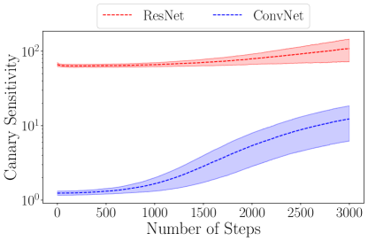
Figure 1: The gradient norm of the canary varies along the optimization path and for different architectures. We report the mean and $\pm 2$ standard deviations across 30 random runs.

Gradient-crafting adversaries. Following the above threat model, we allow the adversary to craft an arbitrary gradient sequence as long as it is not a function of the intermediate models. In other words, the adversary must decide on a sequence of gradients before training starts, in an offline way, to audit a complete, end-to-end training run of DP-SGD. We stress that this is in stark contrast to Nasr et al. [30], who use gradient-crafting adversaries to audit each step of DP-SGD and then leverage composition to derive a privacy lower bound for the overall training run. Their approach thus explicitly relies on the adversary having access to all intermediate models, whereas ours does not make this assumption nor use this information in any way.

Our construction helps to understand the hidden state threat model and its properties by decoupling the privacy leakage induced by a worst-case sequence of gradients from the craftability of a canary that could produce that sequence. Allowing the adversary to craft a gradient sequence directly circumvents two issues in prior attempts to audit the hidden state model [30, 36]:

• Saturating the gradient norm: The canary point crafted by prior adversaries is not guaranteed to saturate the gradient clipping threshold throughout training. The adversary’s performance becomes architecture-dependent: for example, a small convolutional neural network has a small canary norm at the start of the training compared to a ResNet, as observed in Figure 1. Thus, for a tight audit, one must tune the clipping threshold according to the canary gradient norm, a quantity the adversary cannot access in our threat model.

• Hypothesis testing: Prior adversaries need to test the presence of a sequence of gradients they cannot access, so they use the model’s loss as a proxy confidence score (RankSample in Algorithm 1): a lower loss implies a higher confidence that a sample was used during training. By allowing the adversary to pick the sequence of gradients, we can align the choice of confidence score to the way adversarial information is encoded in the gradients (as will be evident in the adversaries we propose below), thereby achieving superior testing performance.

Concrete adversary instantiations. We propose two concrete instantiations of our gradient-crafting adversaries, which we will use to perform privacy auditing on real datasets in the next section (see Appendix C for more precise descriptions):

1. Random Biased Dimension ($\mathcal{A}_{GC}$-R): The adversary picks a random dimension and crafts gradients with magnitude $C$ in this dimension. To test whether crafted gradients were inserted (RankSample in Algorithm 1), the adversary uses the difference between $\theta_{T}$ and $\theta_{0}$ in that dimension as the confidence score (RankSample in Algorithm 1).

2. Simulated Biased Dimension ($\mathcal{A}_{GC}$-S): The adversary simulates the training algorithm and picks the least updated dimension. Then, it crafts gradients with magnitude $C$ in that dimension. To test the presence of crafted gradients, the adversary uses the same confidence score as $\mathcal{A}_{GC}$-R.

5 Privacy Auditing Results on Real Datasets

5.1 Experimental Setup

Training details. We perform auditing on two datasets: we choose CIFAR10 [25] as a representative dataset for the state-of-the-art in differentially private training [37, 12], and Housing [32] to underline the hardness of auditing smaller models in the hidden state. We use predefined hyperparameters for each dataset: on CIFAR10, the batch size is 128, and the learning rate is 0.01, while on Housing, the batch size is 400, and the learning rate is 0.1. Training is done with DP-SGD with no momentum. We use three models: a fully connected neural network (FCNN) for the Housing dataset [32], a convolutional neural network (CovNet) [26] and a residual network (ResNet) [21] for CIFAR10. A detailed description of the models can be found in Appendix D.

Baseline adversary. As baseline, we adopt an adversary used in prior related research [30, 36]. This adversary selects a point from the training dataset and flips its label to generate an outlier which serves as the canary $x^{*}$. The loss of the model on this canary is used as confidence score to test whether it was inserted or not. We refer to this baseline as the "loss-based adversary", denoted by $\mathcal{A}_{L}$.

Privacy accounting & auditing. We compute privacy upper and lower bounds for the crafted gradient (for $\mathcal{A}_{GC}$) or canary ($\mathcal{A}_{L}$) as follows. The theoretical privacy upper bound is obtained with the numerical accountant proposed by Gopi et al. [19]. We audit three scenarios for which the accountant gives equivalent privacy guarantees, inserting the crafted gradient or canary at different periodicity $k\in\{1,5,25\}$ and adjusting the time horizon $T$ accordingly. More precisely, when $k=1$, the model is trained for 250 optimization steps, and the crafted gradient or canary is inserted at every step; when $k=5$, the model is trained for 1250 steps, and insertion occurs every $5$ steps, and similarly for $k=25$. For auditing, we rely on the recently proposed scheme based on Gaussian DP (described in Appendix A for completeness) as it allows accurate auditing with a small number of auditing runs [30]. Details on training and auditing parameters can be found in Appendix D.

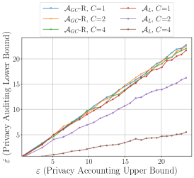
(a) Auditing ConvNet

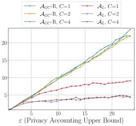
(b) Auditing ResNet

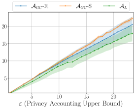
(c) Auditing FCNN.

Figure 2: Auditing results for $\mathcal{A}_{GC}$ (ours) and $\mathcal{A}_{L}$ on ConvNet (Fig. 2a) and ResNets (Fig. 2b) at periodicity $k=1$ and $C\in\{1,2,4\}+$. In Fig. 2c we present the results for $\mathcal{A}_{GC}$-R (ours), $\mathcal{A}_{GC}$-S (ours) and $\mathcal{A}_{L}$ on FCNN (Housing dataset) at periodicity $k=1$.

5.2 Auditing results for periodicity $k=1$

Over-parameterized models. The results in Figure 2 show that our adversary $\mathcal{A}_{GC}$-R achieves tight auditing results in the hidden state model when the crafted gradient is inserted at every step, a result that had been achieved until now only when the adversary could pick a worst-case dataset $D=\{\emptyset\}$ [29] and set the learning rate to $0$ in steps where the canary is not inserted, or when the adversary had access to the intermediate models [30]. Note that the baseline loss-based adversary $\mathcal{A}_{L}$ is indeed not tight and even very loose in some regimes.

The fact that a tight audit can be achieved by our simplest adversary $\mathcal{A}_{GC}$-R (random biased dimension) may seem surprising. We provide a high-level explanation of this phenomenon. As we are auditing over-parameterized models, which are highly redundant, we can expect a genuine gradient to assign on average a magnitude of $\mathcal{O}(\frac{C|\text{minibatch}|}{p})$ to each dimension, where $p$ is the number of parameters of the model. As $p$ is typically orders of magnitude larger than the commonly used batch sizes, genuine gradients in a mini-batch contribute a negligible magnitude to any dimension compared to the magnitude of $C$ inserted at a single dimension by $\mathcal{A}_{GC}$-R (or $\mathcal{A}_{GC}$-S). Therefore, genuine gradients do not interfere with the contribution of the adversary, regardless of the selected dimension. We see below that this no longer holds when auditing low-dimensional models.

Low-dimensional models. Auditing smaller models is more challenging because the ratio between the mini-batch size and the number of parameters is much larger. To evaluate our adversaries in this regime, we switch to the Housing dataset with the FCNN model, which has only 68 parameters. We report the performance of our two adversaries over five independent runs in Figure 2c. We observe that randomly selecting a dimension ($\mathcal{A}_{GC}$-R) no longer achieves tight results, although it still outperforms the baseline loss-based adversary. Remarkably, our second adversary, which simulates the training algorithm to select an appropriate dimension ($\mathcal{A}_{GC}$-S), recovers nearly tight results with small variance between runs.

To conclude, the tightness of our adversaries implies a novel negative result.

Implication 1.

If a data point is used at every optimization step of DP-SGD, hiding intermediate models does not amplify its privacy guarantees.

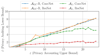
(a) Canary insertion periodicity $k=5$

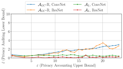
(b) Canary insertion periodicity $k=25$

Figure 3: Auditing results for $\mathcal{A}_{GC}$(ours) and $\mathcal{A}_{L}$ on ConvNet and ResNet (CIFAR10) at privacy parameters $C=1$ at periodicity $k=5$ (Figure 3a) and $k=25$ (Figure 3b).

5.3 Auditing Results at Periodicity $k>1$

We now study how our adversaries perform when the crafted gradient is inserted at a higher periodicity $k\in\{5,25\}$. We observe in Figure 3 that (i) we still outperform the baseline loss-based adversary $\mathcal{A}_{L}$ by a large margin, but (ii) we no longer match the privacy upper bound, and our adversary becomes weaker as we increase $k$. Intuitively, the latter is due to the accumulation of the noise added on genuine gradients during the $k-1$ iterations between each crafted gradient insertion. However, privacy accounting (i.e., the upper bound) does not take advantage of this accumulated noise: as the insertion of a crafted gradient at a given step could bias subsequent genuine gradients towards a particular direction, the best one can do is to resort to the post-processing property of DP, which ensures that subsequent genuine gradients do not weaken the privacy guarantees. In the next section, we investigate whether it is possible to match the upper bound given by privacy accounting in this setting, which amounts to designing an adversary capable of crafting gradients that maximally influence subsequent genuine gradients.

Remark 1.

Using auditing via Gaussian DP [30] for $k>1$ implies approximating the trade-off function of the mechanism with a Gaussian one (see Appendix A for relevant definitions). This approximation can be justified by the Central Limit Theorem [13], and has been used before when auditing the hidden state [30] We show in Appendix E (Figure 8a) that the approximation error is indeed negligible in our case.

6 Towards a Worst-Case Adversary for the Hidden State

In this section, we investigate whether it is possible to reduce (and potentially close) the gap with the theoretical upper bound observed in Section 5.3. For simplicity, we consider the case where a crafted gradient is inserted only in the first optimization step, and then $T-1$ subsequent steps are performed without inserting crafted gradients. This corresponds to the scenario studied by privacy amplification by iteration [18], but we do not restrict ourselves to convex losses.

We introduce a new class of adversaries $\mathcal{A}_{S}$ that crafts the gradient and the loss landscape itself, thereby controlling the distribution of all $T$ updates. Therefore, $\mathcal{A}_{S}$ can pick a (non-convex) loss landscape such that the crafted gradient inserted at step $T=1$ maximally biases subsequent genuine gradients, thereby yielding the highest possible privacy loss for the final model. Note the underlying principle is the same as in Section 4: instead of requiring the adversary to craft a dataset, model architecture and loss function, we allow the adversary to select the loss landscape directly, considering that there could be a dataset that would generate this landscape. As long as the loss landscape is selected before training starts, this is covered by the hidden state threat model we consider.

We formalize the above using the following pair of one-dimensional stochastic processes:

$$\theta_{t+1} =\theta_{t}-g(\theta_{t})+Z_{t+1},$$ (3)

$$\overline{\theta}_{t+1} =\overline{\theta}_{t}-g(\overline{\theta}_{t})+Z_{t+1},$$ (4)

where the first step of the process is either $\theta_{1}=Z_{1}$ (a process that did not use the crafted gradient) or $\overline{\theta}_{1}=\nabla^{*}+Z_{1}$ (a process that used the crafted gradient $\nabla^{*}$), with $Z_{i}\sim\mathcal{N}(0,C^{2}\sigma^{2})$, and $g:\mathbb{R}\rightarrow[-C,C]$ is the function that abstracts the gradient of the loss. The adversary can choose the function $g$ and the crafted gradient $\nabla^{*}$, without knowing the intermediary updates, so as to make the distribution of $\theta_{T}$ and $\overline{\theta}_{T}$ as “distinguishable” as possible.

Example 1 (Constant $g$).

Consider the simple case where $g$ outputs a constant $c$, independent of the input. This implies that the Gaussian noise accumulates at every step, and the privacy loss $\varepsilon$ for the last iterate converges to $0$ as $T\rightarrow\infty$ at a rate of $O(1/\sqrt{T})$.

As illustrated by Example 1, it is easy to design a function $g$ that amplifies privacy over time. However, the converse objective, i.e., designing a function that provides no or minimal privacy amplification for the final step $T$, appears much more challenging.

Figure 4: Comparison between the privacy accounting upper bound and the auditing performance of our adversary $\mathcal{A}^{h_{*}}_{S}$ when $T=2$. All results are averaged across five training runs.

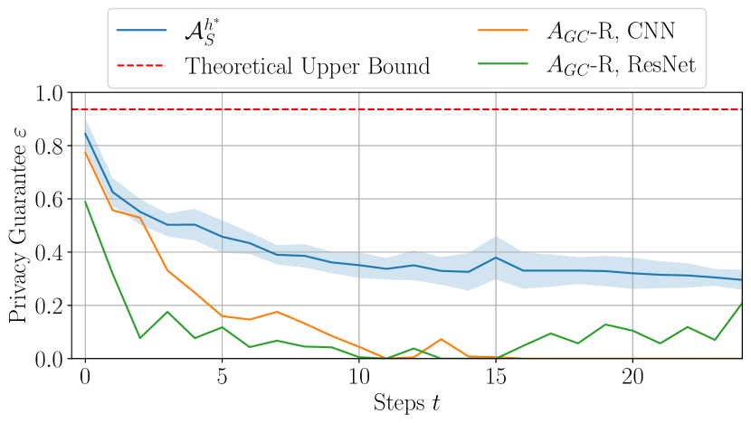
Figure 5: Comparison between the privacy accounting upper bound, $\mathcal{A}^{h_{*}}_{S}$ and $\mathcal{A}_{GC}$-R (ConvNet and ResNet) when $T=25$. The results for $\mathcal{A}^{h_{*}}_{S}$ are averaged across 5 training runs.

A worst-case proposal for $T=2$. We propose a concrete adversary $\mathcal{A}^{h^{*}}_{S}$ which selects $\nabla^{*}=C$ and the function $g_{\phi^{*}}(X)=C\text{ if }\phi^{*}(X)=1\text{ and }g_{\phi^{*}}(X)=-C$ otherwise, where $\phi^{*}:\mathbb{R}\rightarrow\{0,1\}$ is the linear threshold function that achieves the minimal False Positive Error Rate $\alpha$ + False Negative Error Rate $\beta$ for distinguishing between $\theta_{1}$ and $\overline{\theta}_{1}$ (i.e., testing if the model after $1$ step was generated using the crafted gradient $\nabla^{*}$). More precisely, $\phi^{*}(X)=1\text{ if }X>h^{*}\text{ and }\phi^{*}(X)=0$ otherwise, with $h^{*}=\frac{|\nabla^{*}|}{2}=\frac{C}{2}$ (see Appendix F for a numerical validation). The resulting loss landscape adheres to the intuition that the crafted gradient maximally biases the subsequent steps (see Appendix F). We denote this adversary by $\mathcal{A}^{h^{*}}_{S}$, and conjecture that $\mathcal{A}^{h^{*}}_{S}$ is the worst-case adversary for $T=2$.

Figure 5 shows the performance of our adversary $\mathcal{A}_{S}^{h^{*}}$ for $T=2$ (i.e., a single intermediary hidden state). Although its performance comes fairly close to the privacy accounting upper bound, there is still a noticeable gap, providing strong evidence that the hidden state may be able to provide privacy amplification in the non-convex regime for data points that are not used at every optimization step.

Using $\mathcal{A}^{h^{*}}_{S}$ to audit $T>2$. We then use our adversary $\mathcal{A}^{h^{*}}_{S}$ to audit $T=25$ steps The results are shown in Figure 5, where we also report the performance of our previous adversaries $\mathcal{A}_{GC}$ on CIFAR10 in addition to the privacy accounting upper bound. The first important takeaway is that $\mathcal{A}^{h^{*}}_{S}$ outperforms $\mathcal{A}_{GC}$ by a significant margin thanks to its ability to bias subsequent gradients, leading to the following implication.

Implication 2.

Either attacks on realistic datasets can be improved in the hidden state, or common deep neural networks constrain the gradient dynamics in a way that amplifies privacy.

The second key observation is that the privacy loss of $\mathcal{A}^{h^{*}}_{S}$ converges to a constant: this is because the privacy loss distributions become sufficiently far away and stop mixing over time. While this again suggests that some privacy amplification might be possible in the non-convex regime, it implies that this potential amplification must be qualitatively weaker than in the convex case.

Implication 3.

In the non-convex regime, the privacy loss of a sample cannot go to $0$ as subsequent steps are performed, in contrast to the convex case where the privacy loss decreases in $O(1/\sqrt{T})$ [18].

7 Discussion and Future Work

Our work allows tighter auditing of DP-SGD in the hidden state model, and our results yield several important implications that advance the understanding of this threat model. For instance, Implication 3 means that the property of converging privacy loss of DP-SGD as $T\rightarrow+\infty$ recently established by [2] in the convex case cannot hold for non-convex models. Beyond differential privacy, our results have consequences for machine unlearning [7], which aims to remove a specific data point and from a trained model as if the data had never been used for training. A recent approach to unlearning relies on noisy training and privacy amplification by iteration [9]. Implication 3 shows that this approach cannot provide complete data point deletion when considering non-convex models like neural networks.

Beyond these negative results, our work strongly suggests that a (weaker) form of privacy amplification does occur for non-convex problems in the hidden state model. Modelling gradient sequences and loss landscapes, as done in Section 6, could eventually be formalized into a universally worst-case adversary and, ultimately, a better privacy accountant for the hidden state model. Another open question is to understand when and how a gradient can bias the entire optimization path, as well as when and how gradient-crafting adversaries can be achieved through the design of a canary point and a dataset. This has implications regarding the possibility of designing more effective and realistic attacks.

Finally, we note that our threat model and adversaries are well-suited to audit federated learning with partial participation [38]. In this case, the adversary is a client who does not observe the model’s state in rounds where it does not participate. Our approach provides an interesting alternative to existing methods for auditing federated learning, which either assumes the knowledge of all intermediate models (unrealistic under partial participation) [28], or yields loose privacy lower bounds [3].

Appendix A Details on Auditing via Gaussian DP

For completeness, in this section we present the privacy auditing approach proposed by Nasr et al. [30], which we use in our experiments. We start by introducing some necessary concepts on $f$-DP and Gaussian DP in Section A.1. Then, in Section A.2, we present an overview of how auditing is performed and how all the elements of the general auditing pipeline (Algorithm 1) are implemented.

A.1 $f$-Differential Privacy and Gaussian Differential Privacy

$f$-DP and Gaussian DP Dong et al. [13] are based on a characterization of DP as binary hypothesis testing. We recall the main concepts below.

Definition 2 (Error rates).

Let $P$ and $Q$ be two arbitrary distributions and $O$ a sample drawn from either $P$ or $Q$. Let a binary hypothesis test be defined by the following two hypotheses: $H_{0}:$ “the output $O$ is drawn from $P$” or “$H_{1}$: the output $O$ is drawn from $Q$”. Consider a rejection rule $\phi:\mathcal{R}^{d}\rightarrow[0,1]$ that outputs the probability that we should reject $H_{0}$. We define the Type I (or false positive) error rate of this rejection rule $\phi$ as $\alpha_{\phi}\overset{\Delta}{=}\underset{P}{\mathbb{E}}[\phi]$ and the Type II (or false negative) error rate as $\beta_{\phi}\overset{\Delta}{=}1-\underset{Q}{\mathbb{E}}[\phi].$

Definition 3 (Trade-off functions).

Let $P$ and $Q$ be two arbitrary distributions. We define the trade-off function between $P$ and $Q$ as:

$$T(P,Q)(\alpha)=\underset{\phi}{\inf}\{\beta_{\phi}:\alpha_{\phi}\leq\alpha\}.$$ (5)

We can now introduce $f$-DP.

Definition 4 ($f$-Differential Privacy).

Let $f$ be a trade-off function. Then a mechanism $M$ is $f$-Differentially Private ($f$-DP) if for all neighbouring datasets $D$ and $D^{\prime}$:

$$T(M(D),M(D^{\prime}))\geq f.$$ (6)

Trade-off functions describe the lowest Type II error rate achievable by any adversary at any Type I error rate . We say that a mechanism $M_{1}$ is strictly less private than $M_{2}$ if $T(M_{1}(D),M_{1}(D^{\prime}))(\alpha)\leq T(M_{2}(D),M_{2}(D^{\prime}))(\alpha)$ for all $\alpha\in[0,1]$. Dong et al. [13] show $(\epsilon,\delta)$-DP can be formulated as $f$-DP as follows:

$$f_{\epsilon,\delta}(\alpha)=\max\{0,1-\delta e^{\epsilon},e^{-\epsilon}(1-\delta)\}$$ (7)

Gaussian Differential Privacy (GDP) is a specialized formulation of $f$-DP where $f$ is the trade-off function of two Gaussian distributions.

Definition 5 (Gaussian Differential Privacy).

Let $\Phi$ be the cumulative distribution function (CDF) of $\mathcal{N}(0,1)$ and $\Phi^{-1}$ its associated quantile function. A mechanism $M$ is $\mu$-GDP if it is $G_{\mu}$-DP, where

$$G_{\mu}(\alpha)\overset{\Delta}{=}T(M(D),M(D^{\prime}))(\alpha)=\Phi(\Phi^{-1}(1-\alpha)-\mu).$$ (8)

The following result is crucial for auditing: it shows that the error rates of an adversary give a lower bound on the GDP guarantees.

Lemma 1 (Relating error rates to GDP).

Assume that an adversary has error rates $\alpha_{M}$, $\beta_{M}$ in the binary test defined by $P=M(D)$ and $Q=M(D^{\prime})$ where $M$ is a mechanism and $D$ and $D^{\prime}$ are two neighboring datasets. Then, if $M$ satisfies $\mu$-GDP, then

$$\mu\geq\Phi^{-1}(1-\alpha)-\Phi^{-1}(\beta).$$ (9)

Finally, we can convert $\mu$-GDP to $(\epsilon,\delta)$-DP.

Corollary 1 (From $\mu$-GDP to $(\epsilon,\delta)$-Differential Privacy.).

If a mechanism $M$ is $\mu$-GDP then it satisfies $(\epsilon,\delta)$-DP, where:

$$\delta(\epsilon)=\Phi(-\frac{\epsilon}{\mu}+\frac{\mu}{2})-e^{\varepsilon}\Phi(-\frac{\epsilon}{\mu}-\frac{\mu}{2}).$$ (10)

A.2 Auditing via GDP

Auditing a mechanism $M$ via GDP follows the general approach outlined in Algorithm 1, and amounts to instantiating its different primitives:

1. RankSample: We first generate $R$ outputs of $M$, half of them sampled from $M(D)$, the rest from $M(D^{\prime})$, where $D^{\prime}=D\cup\{x^{*}\}$. For each output $i\in\{1,\dots,R\}$, a score $S_{i}$ is computed to the adversary’s confidence that either $D$ or $D^{\prime}$ were used as input for $M$. The precise computation of this confidence score depends on the considered adversary and is abstracted by the RankSample method in Algorithm 1. We refer to Sections 4-5 for details about the RankSample method used by the adversaries we consider.

2. RejectionRule: Each $S_{i}$ is then augmented with its associated ground truth label $b_{i}$, reflecting if a particular sample has been generated from $D$ or $D^{\prime}$. The adversary selects a classifier (RejectionRule in Algorithm 1) that receives the set $S$ as input and needs to classify it against the ground truth label $b$. We stress that DP holds against any choice of such a classifier. Commonly used ones being linear threshold classifiers [30]. Once a threshold classifier has been selected, we evaluate the error rates of the classifier using $S$ and $b$ as the ground truth labels, evaluating the False Negative (FN), False Positive (FP), True Negative (TN), and True Positive (TP) of the classifier.

3. ConfInterval: Using these statistics, we employ the Clopper Pearson [10] confidence intervals over binomial distributions to get a high-probability lower bound on the Type I error rate ($\alpha)$ and Type II error rate ($\beta$) for the adversary’s performance. We note that other techniques exist to compute such confidence intervals [42, 27]; however, the benefits we observed practically were negligible in our case.

4. ConvertToDP: Finally, given access to the lower bounds on the error rates of the adversary, we can compute the lower bound on the privacy loss of a mechanism $M$ in GDP by using Lemma 1, and translate the result to $(\epsilon,\delta)$-DP using Corollary 1.

We stress that this technique offers a lower bound on the privacy loss, while techniques like privacy accounting [1, 19, 14] or composition [16, 23, 13] offer upper bounds on the privacy loss. We call a mechanism tight if a lower bound offered by auditing match the upper bound

Appendix B Summary of Prior Work on Privacy Auditing of DP-SGD

We provide in Table 1 a list of adversaries used in prior work on privacy auditing of DP-SGD along with their key properties: whether they are compatible with the hidden state, whether they achieved a tight audit, and the type of canary they used.

Paper	Adversary	HS	TA	CT
Jagielski et al. [22]	Poisoned Backdoor	✓	✗	Sample
Nasr et al. [29]	API Access	✓	✗	Sample
	Static Adversary	✓	✗	Sample
	Intermediate Poison Attack	✓	✗	Sample
	Adaptive Poisoning Attack	✗	✗	Sample
	Gradient Attack	✗	✗	Gradient
	Malicious Datasets	✗	✓	Gradient
Zanella-Béguelin et al. [42]	Experiment 1	✓	✗	Sample
	Experiment 2	✓	✗	Sample
Maddock et al. [28]	Algorithm 1	✗	✗	Gradient
Nasr et al. [30]	Algorithm 1	✓	✗	Sample
	Algorithm 2	✗	✓	Gradient
Andrew et al. [3]	Algorithm 2	✓	✗	Sample or Gradient
	Algorithm 3	✗	✗	Gradient
Steinke et al. [36]	audit-type=whitebox	✗	✗	Sample or Gradient
	audit-type=blackbox	✓	✗	Sample
Ours	$\mathcal{A}_{GC}$-R, $k=1$	✓	✓	Gradient
	$\mathcal{A}_{GC}$-R, $k>1$	✓	✗	Gradient

Table 1: Summary of adversaries used in prior privacy auditing of DP-SGD. We report whether the adversary is compatible with the hidden state (HS), if the adversary achieves tight audit in the threat model it operates (TA) and the type of canary (CT) used by the adversary (gradient canaries or sample space canaries).

Appendix C Details about our Adversaries $\mathcal{A}_{GC}$

The algorithmic description of our adversaries $\mathcal{A}_{GC}$-R and $\mathcal{A}_{GC}$-S are given in Algorithms 2-3.

We discuss different strategies to select the biased dimension for our adversary $\mathcal{A}_{GC}$-S. The general idea is to explore how the different dimensions are updated by simulating the training process, as all the required knowledge is available to the adversary. We have considered two types of simulations: (i) Noisy simulation, in which we use the same noise variance as the simulated process, and (ii) Noiseless simulation, in which we run the training algorithm without noise or clipping. Note that for the noiseless simulation, the training algorithm is deterministic, as the initialization and the batches are fixed and known to the adversary, while in the noisy simulation, the stochasticity of DP-SGD is concealed for the adversary. We use four simulations of the training process. We then proceed to choose how to rank the most suitable dimension to bias, for which we have explored two options: (i) Per Step (PS): selecting the dimension that has the lowest gradient norm accumulated over all the training runs or (ii) Final Model (FM): selecting the dimension that is the closest to initialization at the end of the training run. We experiment with these design choices, resulting in 4 dimension selection strategies. The results in Figure 7 show that the Noiseless-PS strategy performs best.

In Figure 6, we show that $\mathcal{A}_{GC}$-S using the best strategy is equivalent with $\mathcal{A}_{GC}$-R on our studied over-parameterized models.

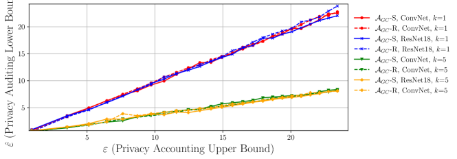
Figure 6: Auditing results for $\mathcal{A}_{GC}$-S compared to $\mathcal{A}_{GC}$-R at $k\in{1,5}$ on ConvNet and ResNet18. We observe that the two adversaries are equivalent for these over-parameterized models, demonstrating that $\mathcal{A}_{GC}$-S only enhances our attack against under-parameterized models.

Algorithm 2 Gradient Generation for $\mathcal{A}_{GC}$-R (Random Biased Dimension)

  Input: dataset $D$, initialization $\theta_{0}\in\mathbb{R}^{p}$, clipping threshold $C$

  $d\leftarrow$ random element from $\{1,\dots,p\}$

  $\nabla^{*}\leftarrow(0,\dots,0)\in\mathbb{R}^{p}$

  $\nabla^{*}[d]\leftarrow C$

  return $\nabla^{*}$

Algorithm 3 Noisy gradient generation for $\mathcal{A}_{GC}$-S (Simulated Biased Dimension)

  Input: dataset $D$, initialization $\theta_{0}\in\mathbb{R}^{p}$, clipping threshold $C$, noise variance $\sigma^{2}$, mini-batches $\{B_{1}\dots B_{T}\}$,           number of runs $r$, parameter selection $\text{rank}\in\{\text{PerStep, FinalModel}\}$, simulation $\in\{\text{Noisy, Noiseless}\}$

  $S=[0]^{p}$

  for $j=1$ to $r$ do

     for $i=1$ to $T$ do

        $Z_{t}\sim\mathcal{N}(0,C^{2}\sigma^{2}\mathbb{I})$

        $\theta_{t+1}\leftarrow\theta_{t}-\frac{\eta}{|B_{t}|}\Big{(}\underset{x\in B_{t}}{\sum}\text{clip}\big{(}{\nabla_{\theta_{t}}}\ell(\theta_{t};x),C\big{)}\Big{)}$

        

        if simulation = Noisy then

           $\theta_{t+1}=\theta_{t+1}+\frac{\eta}{|B_{t}|}Z$, where $Z\sim\mathcal{N}(0,\sigma^{2})$

        end if

        

        if rank = PerStep then

           $S\leftarrow S+\theta_{i}-\theta_{i-1}$

        end if

     end for

     

     if rank = FinalModel then

        $S\leftarrow\theta_{T}-\theta_{0}$

     end if

  end for

  $d\leftarrow\text{argmin }S$

  $\nabla^{*}\leftarrow(0,\dots,0)\in\mathbb{R}^{p}$

  $\nabla^{*}[d]\leftarrow C$

  return $\nabla^{*}$

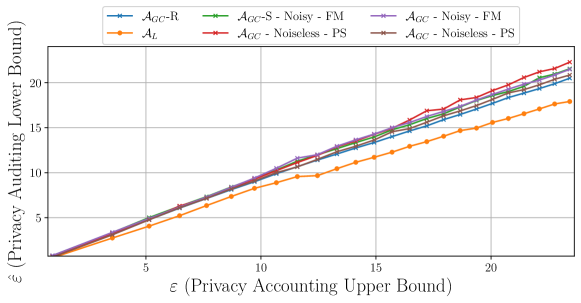
Figure 7: Auditing results of $\mathcal{A}_{L}$, $\mathcal{A}_{GC}$-R and $\mathcal{A}_{GC}$-S on the Housing dataset. We consider 4 variants of $\mathcal{A}_{GC}$-S, depending on whether the noisy or noiseless simulation is used and whether we rank dimensions based on accumulating per-step updates (PS) or on the final model norm difference (FM).

Appendix D Experimental Details on Training & Auditing

In our experimental section, we audit three neural network architectures, a ConvNet and a ResNet on the CIFAR10 dataset and a Fully-Connected Neural Network on the Housing dataset. These models were implemented using PyTorch [33], and the DP-SGD optimizer was Opacus [41]. The hyperparameters for training, privacy guarantees, and privacy auditing parameters for each audited machine learning model are meticulously outlined in Table 2. The ConvNet and ResNet have been audited when trained for 250, 1250, and 6250 optimization steps, totalling approximately 3500 GPU hours.

For each experiment, we audit $R=5000$ machine learning models using GDP auditing (see Appendix A). For the Clopper Pearson confidence intervals, we use a confidence of $95\%$ (consistent with prior work [22, 29]) to get a lower bound on the Type I error rate ($\alpha)$ and Type II error rate ($\beta$) for the adversary’s performance. RejectionRule is computed by selecting the best linear threshold classifier on $S$. While, in practice, the adversary should pick the classifier on a set of held-out scores $S$, we select the classifier directly on $S$ to save the computational resources required to compute the held-out set $S$. We stress that it is not an issue, as differential privacy guarantees hold against any choice of classifier.

Table 2: Hyperparameters used per model

Hyperparameter	Fully-Connected NN	ConvNet	ResNet18
Learning rate ($\eta$)	$10^{-2}$	$10^{-2}$	$10^{-2}$
Batch size	400	128	128
Trainable params	68	62006	11173962
Loss Function	Binary Cross Entropy	Cross Entropy	Cross Entropy
Clipping norm $C$	1.0	{ 1.0, 2.0, 4.0 }	{1.0, 2.0, 4.0 }
Noise variance $\sigma$	4	4	4
Failure probability $\delta$	$10^{-5}$	$10^{-5}$	$10^{-5}$
Auditing runs	5000	5000	5000
Confidence Interval	0.95	0.95	0.95

Appendix E Approximation Errors for GDP Auditing

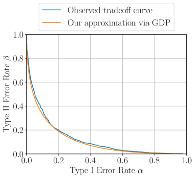
(a) The approximation error of approximating the tradeoff function of the observations via GDP for $\mathcal{A}_{GC}$-R when auditing a ConvNet on CIFAR10 when $k=5$ at step 1250.

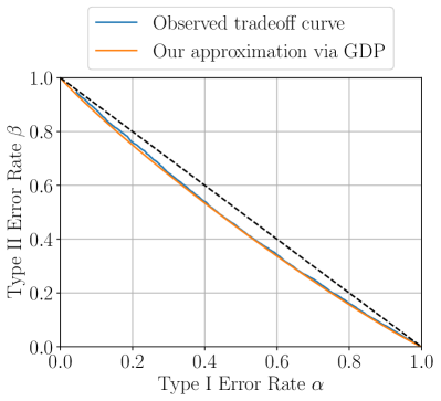
(b) The approximation error of approximating the tradeoff function of the observations via GDP for $\mathcal{A}^{h^{*}}_{S}$ when the $T=25$ case at privacy parameter $C=1$ and $\sigma=4$.

As explained in Remark 1, using auditing via Gaussian DP [30] (see Appendix A) implies approximating the trade-off function of our mechanism with a Gaussian one [13]. In this section, we present some samples of the privacy trade-off curves that we observe when auditing both $\mathcal{A}_{GC}$ in Figure 8a and $\mathcal{A}^{h^{*}}_{S}$ in Figure 8b. For $\mathcal{A}_{GC}$, we show the case where $T=1250$ when auditing a ConvNet at canary gradient insertion periodicity $k=5$ on CIFAR10, while for $\mathcal{A}^{h^{*}}_{S}$ we present the approximation when $T=25$. We see that the approximation errors are negligible, and the approximation technique is representative.

This good behavior is due to the Central Limit Theorem for $f$-DP composition [13], which, in a nutshell, states that while individual mechanisms are not well approximated by a Gaussian Mechanism, their composition has a decaying error in the number of compositions performed when approximated via a Gaussian Mechanism.

Appendix F Details on our adversary $\mathcal{A}^{*}_{h}$

Visualization of the loss landscape. Figure 8 shows the loss landscape corresponding to our adversary $\mathcal{A}^{*}_{h}$ defined in Section 6. One can see how the crafted gradient is able to bias subsequent steps. Note that the discontinuity is not essential and can be removed by appropriate scaling.

Numerical validation of optimality of $h^{*}$. In this section, we numericalli validate that the choice of threshold $h^{*}$ in $\mathcal{A}^{h^{*}}_{S}$ is indeed optimal for $T=2$ by comparing it with all possible threshold functions. To search for these functions, we discretize the Type I error rate $\alpha\in[0,1]$ into $\{\alpha_{1}\dots\alpha_{d}\}$, and each $\alpha_{i}$ we look for the rejection rule $\phi_{i}$ that achieves the lowest Type II error rate $\beta_{i}$. Given that, in this case, our function $g$ distinguishes between two Gaussian distributions via Neyman-Pearson [31], it is well known that the optimal classifier with a fixed type I error rate is achieved by its associated threshold classifier $h_{i}=\Phi(1-\alpha_{i})$, where $\Phi$ is the CDF of $\mathcal{N}(0,\sigma^{2})$. With $\{h_{1}\dots h_{d}\}$ at hand, we can define multiple $g_{\phi_{i}}$, and implicitly multiple adversaries $\mathcal{A}^{h_{i}}_{S}$ that use $g_{\phi_{i}}$ as a candidate for $g$ in Eq. 3 which we use to audit, resulting in $\{\hat{\epsilon}_{1}\dots\hat{\epsilon}_{d}\}$, out of which we pick the maximum. A detailed description is provided in Algorithm 5.

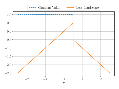
Figure 8: Visualization of the loss landscape corresponding to $A^{h^{*}}_{S}$ for clipping threshold $C=1$.

The results shown in Figure 9 confirm that $\mathcal{A}^{h^{*}}_{S}$ employs the optimal threshold classifier to distinguish the input distributions.

Algorithm 4 Lower Bound Search

  $\{\alpha_{1}\dots\alpha_{d}\}=\text{linspace}(0,\Phi(\frac{C}{2\sigma^{2}}),d)$

  for $\alpha_{i}$ $\in$ $\{\alpha_{1}\dots\alpha_{d}\}$ do

     $h_{i}=\Phi^{-1}(1-\alpha_{i})$

     $\hat{\varepsilon}$ = Audit($g_{\phi_{h_{i}}}$)

  end for

  return $\max(\hat{\varepsilon})$

Algorithm 5 Search routine over multiple threshold classifiers.

Figure 9: Comparison between the privacy accounting upper bound and the auditing performance of $\mathcal{A}^{h^{*}}_{S}$ and our threshold search algorithm when $T=2$. All results are averaged across five training runs

References

- Abadi et al. [2016] Martin Abadi, Andy Chu, Ian Goodfellow, H. Brendan McMahan, Ilya Mironov, Kunal Talwar, and Li Zhang. Deep learning with differential privacy. In Proceedings of the 2016 ACM SIGSAC Conference on Computer and Communications Security (CCS), 2016.
- Altschuler and Talwar [2022] Jason M. Altschuler and Kunal Talwar. Privacy of noisy stochastic gradient descent: More iterations without more privacy loss. In NeurIPS, 2022.
- Andrew et al. [2024] Galen Andrew, Peter Kairouz, Sewoong Oh, Alina Oprea, H. Brendan McMahan, and Vinith Suriyakumar. One-shot empirical privacy estimation for federated learning. In ICLR, 2024.
- Balle et al. [2019] Borja Balle, Gilles Barthe, Marco Gaboardi, and Joseph Geumlek. Privacy amplification by mixing and diffusion mechanisms. In NeurIPS, 2019.
- Balle et al. [2022] Borja Balle, Giovanni Cherubin, and Jamie Hayes. Reconstructing training data with informed adversaries. In IEEE Symposium on Security and Privacy (S&P), 2022.
- Bassily et al. [2014] Raef Bassily, Adam D. Smith, and Abhradeep Thakurta. Private Empirical Risk Minimization: Efficient Algorithms and Tight Error Bounds. In FOCS, 2014.
- Bourtoule et al. [2021] Lucas Bourtoule, Varun Chandrasekaran, Christopher A Choquette-Choo, Hengrui Jia, Adelin Travers, Baiwu Zhang, David Lie, and Nicolas Papernot. Machine unlearning. In 2021 IEEE Symposium on Security and Privacy (SP), pages 141–159. IEEE, 2021.
- Carlini et al. [2022] Nicholas Carlini, Steve Chien, Milad Nasr, Shuang Song, Andreas Terzis, and Florian Tramer. Membership inference attacks from first principles. In IEEE Symposium on Security and Privacy (S&P), pages 1897–1914. IEEE, 2022.
- Chien et al. [2024] Eli Chien, Haoyu Wang, Ziang Chen, and Pan Li. Stochastic gradient langevin unlearning. arXiv preprint arXiv:2403.17105, 2024.
- Clopper and Pearson [1934] C. J. Clopper and E. S. Pearson. The use of Confidence or Fiducial Limits Illustrated in the Case of the Binomial. Biometrika, 1934.
- Cyffers and Bellet [2022] Edwige Cyffers and Aurélien Bellet. Privacy amplification by decentralization. In AISTATS, 2022.
- De et al. [2022] Soham De, Leonard Berrada, Jamie Hayes, Samuel L Smith, and Borja Balle. Unlocking high-accuracy differentially private image classification through scale. arXiv preprint arXiv:2204.13650, 2022.
- Dong et al. [2022] Jinshuo Dong, Aaron Roth, and Weijie J. Su. Gaussian differential privacy. Journal of the Royal Statistical Society: Series B (Statistical Methodology), 84(1):3–37, 2022.
- Doroshenko et al. [2022] Vadym Doroshenko, Badih Ghazi, Pritish Kamath, Ravi Kumar, and Pasin Manurangsi. Connect the dots: Tighter discrete approximations of privacy loss distributions. In Privacy Enhancing Technologies Symposium (PETS), 2022.
- Dwork and Roth [2014] Cynthia Dwork and Aaron Roth. The Algorithmic Foundations of Differential Privacy. Foundations and Trends® in Theoretical Computer Science, 9(3–4):211–407, 2014.
- Dwork et al. [2006] Cynthia Dwork, Frank McSherry, Kobbi Nissim, and Adam Smith. Calibrating noise to sensitivity in private data analysis. In Shai Halevi and Tal Rabin, editors, Theory of Cryptography, pages 265–284, Berlin, Heidelberg, 2006. Springer Berlin Heidelberg. ISBN 978-3-540-32732-5.
- Erlingsson et al. [2019] Úlfar Erlingsson, Vitaly Feldman, Ilya Mironov, Ananth Raghunathan, Kunal Talwar, and Abhradeep Thakurta. Amplification by shuffling: From local to central differential privacy via anonymity. In SODA, 2019.
- Feldman et al. [2018] Vitaly Feldman, Ilya Mironov, Kunal Talwar, and Abhradeep Thakurta. Privacy amplification by iteration. In FOCS, 2018.
- Gopi et al. [2021] Sivakanth Gopi, Yin Tat Lee, and Lukas Wutschitz. Numerical composition of differential privacy. In NeurIPS, 2021.
- Haim et al. [2022] Niv Haim, Gal Vardi, Gilad Yehudai, Ohad Shamir, and Michal Irani. Reconstructing training data from trained neural networks. In NeurIPS, 2022.
- He et al. [2016] Kaiming He, Xiangyu Zhang, Shaoqing Ren, and Jian Sun. Deep residual learning for image recognition. In Proceedings of the IEEE conference on computer vision and pattern recognition, 2016.
- Jagielski et al. [2020] Matthew Jagielski, Jonathan Ullman, and Alina Oprea. Auditing differentially private machine learning: How private is private sgd? Advances in Neural Information Processing Systems, 33:22205–22216, 2020.
- Kairouz et al. [2015] Peter Kairouz, Sewoong Oh, and Pramod Viswanath. The composition theorem for differential privacy. In ICML, pages 1376–1385. PMLR, 2015.
- Kasiviswanathan et al. [2011] Shiva Prasad Kasiviswanathan, Homin K. Lee, Kobbi Nissim, Sofya Raskhodnikova, and Adam Smith. What can we learn privately? SIAM Journal on Computing, 40(3):793–826, 2011.
- Krizhevsky [2009] Alex Krizhevsky. Learning multiple layers of features from tiny images. 2009.
- LeCun et al. [1989] Y. LeCun, B. Boser, J. S. Denker, D. Henderson, R. E. Howard, W. Hubbard, and L. D. Jackel. Backpropagation applied to handwritten zip code recognition. Neural Computation, 1(4):541–551, 1989. doi: 10.1162/neco.1989.1.4.541.
- Lu et al. [2022] Fred Lu, Joseph Munoz, Maya Fuchs, Tyler LeBlond, Elliott Zaresky-Williams, Edward Raff, Francis Ferraro, and Brian Testa. A general framework for auditing differentially private machine learning. In S. Koyejo, S. Mohamed, A. Agarwal, D. Belgrave, K. Cho, and A. Oh, editors, Advances in Neural Information Processing Systems, volume 35, pages 4165–4176. Curran Associates, Inc., 2022.
- Maddock et al. [2023] Samuel Maddock, Alexandre Sablayrolles, and Pierre Stock. CANIFE: Crafting canaries for empirical privacy measurement in federated learning. In The Eleventh International Conference on Learning Representations, 2023.
- Nasr et al. [2021] Milad Nasr, Shuang Songi, Abhradeep Thakurta, Nicolas Papernot, and Nicholas Carlin. Adversary instantiation: Lower bounds for differentially private machine learning. In 2021 IEEE Symposium on security and privacy (SP), pages 866–882. IEEE, 2021.
- Nasr et al. [2023] Milad Nasr, Jamie Hayes, Thomas Steinke, Borja Balle, Florian Tramèr, Matthew Jagielski, Nicholas Carlini, and Andreas Terzis. Tight auditing of differentially private machine learning. 2023.
- Neyman et al. [1933] Jerzy Neyman, Egon Sharpe Pearson, and Karl Pearson. Ix. on the problem of the most efficient tests of statistical hypotheses. Philosophical Transactions of the Royal Society of London. Series A, Containing Papers of a Mathematical or Physical Character, 231(694-706):289–337, 1933. doi: 10.1098/rsta.1933.0009.
- Pace and Barry [1997] R Kelley Pace and Ronald Barry. Sparse spatial autoregressions. Statistics & Probability Letters, 33(3):291–297, 1997.
- Paszke et al. [2019] Adam Paszke, Sam Gross, Francisco Massa, Adam Lerer, James Bradbury, Gregory Chanan, Trevor Killeen, Zeming Lin, Natalia Gimelshein, Luca Antiga, et al. Pytorch: An imperative style, high-performance deep learning library. Advances in neural information processing systems, 32, 2019.
- Shokri et al. [2017] Reza Shokri, Marco Stronati, Congzheng Song, and Vitaly Shmatikov. Membership inference attacks against machine learning models. In 2017 IEEE Symposium on Security and Privacy (SP), pages 3–18, 2017. doi: 10.1109/SP.2017.41.
- Song et al. [2013] Shuang Song, Kamalika Chaudhuri, and Anand D. Sarwate. Stochastic gradient descent with differentially private updates. In 2013 IEEE Global Conference on Signal and Information Processing, pages 245–248, 2013. doi: 10.1109/GlobalSIP.2013.6736861.
- Steinke et al. [2023] Thomas Steinke, Milad Nasr, and Matthew Jagielski. Privacy auditing with one (1) training run. In NeurIPS, 2023.
- Tramèr and Boneh [2021] Florian Tramèr and Dan Boneh. Differentially private learning needs better features (or much more data). In ICLR, 2021.
- Yang et al. [2021] Haibo Yang, Minghong Fang, and Jia Liu. Achieving linear speedup with partial worker participation in non-iid federated learning. In ICLR, 2021.
- Ye and Shokri [2022] Jiayuan Ye and Reza Shokri. Differentially private learning needs hidden state (or much faster convergence). Advances in Neural Information Processing Systems, 35:703–715, 2022.
- Yeom et al. [2018] Samuel Yeom, Irene Giacomelli, Matt Fredrikson, and Somesh Jha. Privacy risk in machine learning: Analyzing the connection to overfitting. In 2018 IEEE 31st computer security foundations symposium (CSF), pages 268–282. IEEE, 2018.
- Yousefpour et al. [2021] Ashkan Yousefpour, Igor Shilov, Alexandre Sablayrolles, Davide Testuggine, Karthik Prasad, Mani Malek, John Nguyen, Sayan Ghosh, Akash Bharadwaj, Jessica Zhao, Graham Cormode, and Ilya Mironov. Opacus: User-friendly differential privacy library in PyTorch. arXiv preprint arXiv:2109.12298, 2021.
- Zanella-Béguelin et al. [2023] Santiago Zanella-Béguelin, Lukas Wutschitz, Shruti Tople, Ahmed Salem, Victor Rühle, Andrew Paverd, Mohammad Naseri, Boris Köpf, and Daniel Jones. Bayesian estimation of differential privacy, 2023.
- Zarifzadeh et al. [2023] Sajjad Zarifzadeh, Philippe Liu, and Reza Shokri. Low-cost high-power membership inference by boosting relativity, 2023. arXiv:2312.03262.