Bayesian Adaptive Calibration and Optimal Design

Abstract

The process of calibrating computer models of natural phenomena is essential for applications in the physical sciences, where plenty of domain knowledge can be embedded into simulations and then calibrated against real observations. Current machine learning approaches, however, mostly rely on rerunning simulations over a fixed set of designs available in the observed data, potentially neglecting informative correlations across the design space and requiring a large amount of simulations. Instead, we consider the calibration process from the perspective of Bayesian adaptive experimental design and propose a data-efficient algorithm to run maximally informative simulations within a batch-sequential process. At each round, the algorithm jointly estimates the parameters of the posterior distribution and optimal designs by maximising a variational lower bound of the expected information gain. The simulator is modelled as a sample from a Gaussian process, which allows us to correlate simulations and observed data with the unknown calibration parameters. We show the benefits of our method when compared to related approaches across synthetic and real-data problems.

1 Introduction

In many scientific and engineering disciplines, computer simulation models form an essential part of the process of predicting and reasoning about complex phenomena, especially when real data is scarce. These simulation models depend on the inputs set by the user, commonly referred to as designs, and on a number of parameters representing unknown physical quantities, known as calibration parameters. The problem of setting these parameters so as to closely match observations of the real phenomenon is known as the calibration of computer models.

The seminal work by [Kennedy2001] introduces the Bayesian framework for calibration of simulation models, using Gaussian processes (GPs) [Rasmussen2006], accounting both for the differences between the model and the reality, as well as for uncertainty in the calibration parameters. While the simulator is an essential tool when obtaining real data is expensive or unfeasible, each run of a simulator may itself involve significant computational resources, especially in applications such as climate science or complex engineering systems. In this situation, it is imperative to run simulations at carefully chosen settings of designs as well as of calibration inputs, using current knowledge to optimise resource use [Gutmann2016, Leatherman2017, Marmin2022].

In this contribution, we bridge Bayesian calibration with adaptive experimental design [Rainforth2024] and use information-theoretic criteria [Cover2005] to guide the selection of simulation settings so that they are most informative about the true value of the calibration parameters. We refer to our approach as BACON (Bayesian Adaptive Calibration and Optimal desigN). BACON allows computational resources to be focused on simulations that provide the most value in terms of reducing epistemic uncertainty. Importantly, in contrast to prior work, it optimises designs jointly with calibration inputs in order to capture informative correlations across both spaces. Experimental results on synthetic experiments and a robotic gripper design problem demonstrate the benefits of BACON compared to competitive baselines in terms of computational savings and the quality of the estimated posterior under similar computational constraints.

2 Problem Formulation

Let $f:\mathcal{X}\to{\mathcal{{Y}}}$ represent a mapping of experimental designs ${\boldsymbol{\mathbf{x}}}\in\mathcal{X}$ to the outcomes of a physical process $f({\boldsymbol{\mathbf{x}}})\in{\mathcal{{Y}}}\subset\mathbb{{R}}$. We are given a set of observed outcomes ${\boldsymbol{\mathbf{y}}}_{R}=[y_{1},\dots,y_{R}]^{\mathsf{T}}$ and their associated designs $\mathcal{X}_{R}:=\{{\boldsymbol{\mathbf{x}}}_{i}\}_{i=1}^{R}\subset\mathcal{X}$. Observations are corrupted by noise as $y_{i}=f({\boldsymbol{\mathbf{x}}}_{i})+\nu_{i}$, where $\nu_{i}\sim\mathcal{N}(0,\sigma_{\nu}^{2})$ is zero-mean Gaussian noise, for $i\in\{1,\dots,R\}$. In addition, we have access to the output of a computer model $h:\mathcal{X}\times\Theta\to\mathbb{{R}}$ given a design input and simulation parameters. Given an optimal setting for the calibration parameters ${\boldsymbol{\mathbf{\theta}}}^{*}\in\Theta$, the simulator $h({\boldsymbol{\mathbf{x}}},{\boldsymbol{\mathbf{\theta}}}^{*})$, can be used to approximate the outcomes of the real physical process $f({\boldsymbol{\mathbf{x}}})$. However, ${\boldsymbol{\mathbf{\theta}}}^{*}$ is unknown, and evaluations of the simulator $h$ are costly, though cheaper than executing real experiments evaluating $f$. Our task is to optimally estimate ${\boldsymbol{\mathbf{\theta}}}^{*}$ given the real data ${\boldsymbol{\mathbf{y}}}_{R}$, outputs of the simulator $h$ and a prior distribution $p({\boldsymbol{\mathbf{\theta}}}^{*})$, representing initial assumptions about ${\boldsymbol{\mathbf{\theta}}}^{*}$.

More concretely, let ${\boldsymbol{\mathbf{\hat{y}}}}_{S}:=[h({\boldsymbol{\mathbf{\hat{{\boldsymbol{\mathbf{x}}}}}}}_{i},{\boldsymbol{\mathbf{\hat{\theta}}}}_{i})]_{i=1}^{S}$ represent simulated outcomes for a set of designs $\widehat{\mathcal{X}}_{S}:=\{{\boldsymbol{\mathbf{\hat{{\boldsymbol{\mathbf{x}}}}}}}_{i}\}_{i=1}^{S}\subset\mathcal{X}$ and simulation parameters $\widehat{\Theta}_{S}:=\{{\boldsymbol{\mathbf{\hat{\theta}}}}_{i}\}_{i=1}^{S}\subset\Theta$. Given the cost of running simulations, we will associate the simulator $h$ with a latent function (usually referred to as emulator) drawn from a Gaussian process (GP) prior and assume simulation outputs and real data follow a joint probability distribution $p({\boldsymbol{\mathbf{y}}}_{R},{\boldsymbol{\mathbf{\hat{y}}}}_{S},{\boldsymbol{\mathbf{\theta}}}^{*})$.

In this setting, the Bayesian experimental design objective is to propose a sequence of simulations which will maximise the expected information gain (EIG) about ${\boldsymbol{\mathbf{\theta}}}^{*}$:

$$\begin{split}&\mathrm{EIG}(\widehat{\mathcal{X}}_{S},\widehat{\Theta}_{S})\\ &:=\mathbb{H}(p({\boldsymbol{\mathbf{\theta}}}^{*}|{\boldsymbol{\mathbf{y}}}_{R}))-\mathbb{E}_{p({\boldsymbol{\mathbf{\hat{y}}}}_{S}|\widehat{\mathcal{X}}_{S},\widehat{\Theta}_{S},{\boldsymbol{\mathbf{y}}}_{R})}[\mathbb{H}(p({\boldsymbol{\mathbf{\theta}}}^{*}|{\boldsymbol{\mathbf{y}}}_{R},{\boldsymbol{\mathbf{\hat{y}}}}_{S}))]\\ &=\mathbb{E}_{p({\boldsymbol{\mathbf{\hat{y}}}}_{S}|\widehat{\mathcal{X}}_{S},\widehat{\Theta}_{S},{\boldsymbol{\mathbf{y}}}_{R})}\left[\mathbb{D}_{\mathrm{KL}}(p({\boldsymbol{\mathbf{\theta}}}^{*}|{\boldsymbol{\mathbf{y}}}_{R},{\boldsymbol{\mathbf{\hat{y}}}}_{S})||p({\boldsymbol{\mathbf{\theta}}}^{*}|{\boldsymbol{\mathbf{y}}}_{R}))\right]\\ &=\mathbb{I}({\boldsymbol{\mathbf{\theta}}}^{*};{\boldsymbol{\mathbf{\hat{y}}}}_{S}\mid{\boldsymbol{\mathbf{y}}}_{R},\widehat{\mathcal{X}}_{S},\widehat{\Theta}_{S})\,,\end{split}$$ (2)

where $\mathbb{H}(\cdot)$ represents the entropy of a probability distribution, $\mathbb{D}_{\mathrm{KL}}(\cdot||\cdot)$ denotes the Kullback-Leibler divergence, and $\mathbb{I}({\boldsymbol{\mathbf{\theta}}}^{*};{\boldsymbol{\mathbf{\hat{y}}}}_{S}\mid{\boldsymbol{\mathbf{y}}}_{R})$ is the mutual information between ${\boldsymbol{\mathbf{\theta}}}^{*}$ and the simulator output ${\boldsymbol{\mathbf{\hat{y}}}}_{S}$ given the real observations ${\boldsymbol{\mathbf{y}}}_{R}$ and the simulator inputs to be optimized. We note here that, in our setting, the real observations ${\boldsymbol{\mathbf{y}}}_{R}$ are always fixed. Therefore, intuitively, the EIG above captures the reduction in uncertainty will be obtained when selecting $(\widehat{\mathcal{X}}_{S},\widehat{\Theta}_{S})$ averaged over all the possible outcomes ${\boldsymbol{\mathbf{\hat{y}}}}_{S}$.

3 Related work

Our work consists of deriving a Bayesian adaptive experimental design approach to the problem of calibration. Therefore, in the following, we will briefly discuss current literature on these two main research areas.

3.1 Adaptive Experimental Design

The problem of experimental design has a long history [Fisher1935], spanning from classical fixed design patterns to modern adaptive approaches [Greenhill2020]. Optimal experimental design consists of selecting experiments which will maximise some form of criterion involving a measure of utility of the experiment and its associated costs [Kiefer1959oed]. Under the Bayesian formulation, uncertainty in the outcomes of the process is considered, and the optimality of a design is measured in terms of its expected utility [Chaloner1995]. Information theory then allows us to quantify information gain as a utility function, which is commonly applied in modern approaches to Bayesian experimental design [Ryan2016].

The estimation of posterior distributions becomes a computational bottleneck for information-theoretic Bayesian frameworks. Recent work has focused on addressing the difficulties in estimating the expected information gain by means of, e.g., variational inference [Foster2019], density-ratio estimation [Kleinegesse2019], importance sampling [Beck2018laplace], and the learning of efficient policies to propose designs [Foster2021, Blau2022]. These methods, however, usually assume that the simulator is known and inexpensive to evaluate. In contrast, we assume simulations come from an expensive black-box function, which we model as a Gaussian process. We refer the reader to the recent review on modern Bayesian methods for experimental design by rainforth2023modern.

3.2 Active Learning for Calibration

Experimental design approaches generally aim towards the selection of designs for physical experiments, whereas we are concerned with the problem of running optimal simulated experiments for model calibration in the presence of real data. When simulations are resource-intensive, a few methods have been derived based on the Bayesian calibration framework proposed by Kennedy2001. Busby2008 present an algorithm to learn GP emulators for a simulator which can then be combined with Bayesian inference algorithms, such as Markov chain Monte Carlo [Andrieu2003], to provide a posterior distribution over parameters. In their approach, the optimised variables are solely the calibration parameters, and the selection criterion is based on minimising the integrated mean-square error of the GP predictions. Many other approaches can be applied to this setting by modelling the simulator or its associated likelihood function as a GP, including Bayesian optimisation [Gutmann2016, Sarkar2019, Oliveira2021] and methods for adaptive Bayesian quadrature [Acerbi2020, Jarvenpaa2020]. Besides GPs, other algorithms based on selecting calibration parameters have been derived using ensembles of neural networks [Cevik2016] and deep reinforcement learning [Tian2022]. These frameworks, however, do not allow for the selection of design points, keeping them fixed.

Allowing for design point decisions to be included, Leatherman2017 presented approaches for combined simulation and physical experimental design based on geometric and prediction-error-based criteria, but using an offline, non-sequential framework. More recently, Marmin2022 derived a deep Gaussian process [Damianou2013] framework for Bayesian calibration problems and presented an application to experimental design among other examples. Their experimental design approach to calibration was based on minimising the variance of the posterior over the unknown parameters. The posterior was modelled as a Gaussian via a Laplace approximation using a lower bound of the GP’s marginal likelihood w.r.t. the parameters. In contrast, we aim to directly estimate a full, free-form posterior distribution over the unknown calibration parameters.

4 Gaussian processes for Bayesian calibration

To estimate information gain, we need a probabilistic model which can correlate simulations with real data and the unknown parameters ${\boldsymbol{\mathbf{\theta}}}^{*}$. Ideally, the model needs to allow for a computationally tractable conditioning on the parameters ${\boldsymbol{\mathbf{\theta}}}^{*}$ and account for the differences between real and simulated data. Hence, we follow the Bayesian calibration approach in Kennedy2001 and model:

$$f({\boldsymbol{\mathbf{x}}})=\rho h({\boldsymbol{\mathbf{x}}},{\boldsymbol{\mathbf{\theta}}}^{*})+\varepsilon({\boldsymbol{\mathbf{x}}})\,,\quad{\boldsymbol{\mathbf{x}}}\in\mathcal{X},\quad{\boldsymbol{\mathbf{\theta}}}^{*}\sim p({\boldsymbol{\mathbf{\theta}}}^{*}),$$ (3)

where $\varepsilon:\mathcal{X}\to\mathbb{{R}}$ represents the error (or discrepancy) between simulations and real outcomes, and $\rho\in\mathbb{{R}}$ accounts for possible differences in scale. We place Gaussian process priors on the simulator $h\sim\mathcal{GP}(0,\hat{k})$ and on the error function $\varepsilon\sim\mathcal{GP}(0,k_{\varepsilon})$.

4.1 Bi-fidelity exact Gaussian process model

Since both $h$ and $\varepsilon$ are GPs, simulations and real outcomes can be jointly modelled as a single Gaussian process. In fact, both the simulator $h$ and the true function $f$ can be seen as different levels of fidelity of the same underlying process, with $h$ representing a coarser version of $f$. Let $s\in{\mathcal{{S}}}:=\{0,1\}$ denote a fidelity parameter. The combined model is then given by:

$$\hat{f}({\boldsymbol{\mathbf{x}}},{\boldsymbol{\mathbf{\theta}}},s):=\begin{cases}h({\boldsymbol{\mathbf{x}}},{\boldsymbol{\mathbf{\theta}}}),\quad&s=0\\ \rho h({\boldsymbol{\mathbf{x}}},{\boldsymbol{\mathbf{\theta}}})+\varepsilon({\boldsymbol{\mathbf{x}}}),\quad&s=1\,.\end{cases}$$ (4)

such that $f({\boldsymbol{\mathbf{x}}})=\hat{f}({\boldsymbol{\mathbf{x}}},{\boldsymbol{\mathbf{\theta}}}^{*},1)$ and $h({\boldsymbol{\mathbf{\hat{{\boldsymbol{\mathbf{x}}}}}}},{\boldsymbol{\mathbf{\hat{\theta}}}})=\hat{f}({\boldsymbol{\mathbf{\hat{{\boldsymbol{\mathbf{x}}}}}}},{\boldsymbol{\mathbf{\hat{\theta}}}},0)$, for any ${\boldsymbol{\mathbf{x}}},{\boldsymbol{\mathbf{\hat{{\boldsymbol{\mathbf{x}}}}}}}\in\mathcal{X}$ and ${\boldsymbol{\mathbf{\hat{\theta}}}}\in\Theta$. As a result, for arbitrary points in the joint space ${\boldsymbol{\mathbf{z}}},{\boldsymbol{\mathbf{z}}}^{\prime}\in{\mathcal{{Z}}}:=\mathcal{X}\times\Theta\times{\mathcal{{S}}}$, the following covariance function parameterises the combined GP model $\hat{f}\sim\mathcal{GP}(0,k)$:

$$\begin{split}k({\boldsymbol{\mathbf{z}}},{\boldsymbol{\mathbf{z}}}^{\prime}):=k_{\rho}(s,s^{\prime})\hat{k}(({\boldsymbol{\mathbf{x}}},{\boldsymbol{\mathbf{\theta}}}),({\boldsymbol{\mathbf{x}}}^{\prime},{\boldsymbol{\mathbf{\theta}}}^{\prime}))+ss^{\prime}k_{\varepsilon}({\boldsymbol{\mathbf{x}}},{\boldsymbol{\mathbf{x}}}^{\prime})\end{split}$$ (5)

where $k_{\rho}(s,s^{\prime}):=(1+s(\rho-1))(1+s^{\prime}(\rho-1))$, ${\boldsymbol{\mathbf{z}}}:=({\boldsymbol{\mathbf{x}}},{\boldsymbol{\mathbf{\theta}}},s)$, and ${\boldsymbol{\mathbf{z}}}^{\prime}:=({\boldsymbol{\mathbf{x}}}^{\prime},{\boldsymbol{\mathbf{\theta}}}^{\prime},s^{\prime})$.

4.2 Joint probabilistic model and predictions

Let ${\boldsymbol{\mathbf{{Z}}}}_{R}:={\boldsymbol{\mathbf{{Z}}}}_{R}({\boldsymbol{\mathbf{\theta}}}^{*}):=[({\boldsymbol{\mathbf{x}}}_{i},{\boldsymbol{\mathbf{\theta}}}^{*},1)]_{i=1}^{R}$ represent the set of partially observed inputs for real data ${\boldsymbol{\mathbf{y}}}_{R}$, and let $\widehat{\boldsymbol{\mathbf{{Z}}}}_{S}:=[({\boldsymbol{\mathbf{\hat{{\boldsymbol{\mathbf{x}}}}}}}_{i},{\boldsymbol{\mathbf{\hat{\theta}}}},0)]_{i=1}^{S}$ denote the current set of simulation inputs for the observations ${\boldsymbol{\mathbf{\hat{y}}}}_{S}$. Under the GP prior, the joint probability model $p({\boldsymbol{\mathbf{\hat{y}}}}_{S},{\boldsymbol{\mathbf{y}}}_{R},{\boldsymbol{\mathbf{\theta}}}^{*})$ can be decomposed as:

$$p({\boldsymbol{\mathbf{\hat{y}}}}_{S},{\boldsymbol{\mathbf{y}}}_{R},{\boldsymbol{\mathbf{\theta}}}^{*})=p({\boldsymbol{\mathbf{\hat{y}}}}_{S},{\boldsymbol{\mathbf{y}}}_{R}|{\boldsymbol{\mathbf{\theta}}}^{*})p({\boldsymbol{\mathbf{\theta}}}^{*})=\int_{{\boldsymbol{\mathbf{\hat{f}}}}}p({\boldsymbol{\mathbf{\hat{y}}}}_{S}|{\boldsymbol{\mathbf{\hat{f}}}})p({\boldsymbol{\mathbf{y}}}_{R}|{\boldsymbol{\mathbf{\hat{f}}}},{\boldsymbol{\mathbf{\theta}}}^{*})p({\boldsymbol{\mathbf{\hat{f}}}}|{\boldsymbol{\mathbf{\theta}}}^{*})p({\boldsymbol{\mathbf{\theta}}}^{*}){\mathop{}\operatorname{d}}{\boldsymbol{\mathbf{\hat{f}}}}\,,$$ (6)

where ${\boldsymbol{\mathbf{\hat{f}}}}:=\hat{f}({\boldsymbol{\mathbf{{Z}}}}({\boldsymbol{\mathbf{\theta}}}^{*}))\in\mathbb{{R}}^{R+S}$, and ${\boldsymbol{\mathbf{{Z}}}}({\boldsymbol{\mathbf{\theta}}}^{*}):=\{{\boldsymbol{\mathbf{{Z}}}}_{R}({\boldsymbol{\mathbf{\theta}}}^{*}),\widehat{\boldsymbol{\mathbf{{Z}}}}_{S}\}$ corresponds to the full set of inputs. The GP prior then allows us to model real and simulated outcomes jointly as a Gaussian random vector ${\boldsymbol{\mathbf{\hat{f}}}}$:

$${\boldsymbol{\mathbf{\hat{f}}}}|{\boldsymbol{\mathbf{\theta}}}^{*}\sim\mathcal{N}({\boldsymbol{\mathbf{0}}},{\boldsymbol{\mathbf{{K}}}}({\boldsymbol{\mathbf{\theta}}}^{*})\,,$$ (7)

where ${\boldsymbol{\mathbf{{K}}}}({\boldsymbol{\mathbf{\theta}}}^{*}):=k({\boldsymbol{\mathbf{{Z}}}}({\boldsymbol{\mathbf{\theta}}}^{*}),{\boldsymbol{\mathbf{{Z}}}}({\boldsymbol{\mathbf{\theta}}}^{*}))=[k({\boldsymbol{\mathbf{z}}},{\boldsymbol{\mathbf{z}}}^{\prime})]_{{\boldsymbol{\mathbf{z}}},{\boldsymbol{\mathbf{z}}}^{\prime}\in{\boldsymbol{\mathbf{{Z}}}}({\boldsymbol{\mathbf{\theta}}}^{*})}$ denotes the prior covariance matrix. Assuming a Gaussian noise model for the observations $y=f({\boldsymbol{\mathbf{x}}},{\boldsymbol{\mathbf{\theta}}}^{*})+\varepsilon({\boldsymbol{\mathbf{x}}})+\nu$, with $\nu\sim\mathcal{N}(0,\sigma_{\nu}^{2})$, the marginal distribution over the observations ${\boldsymbol{\mathbf{y}}}:=[{\boldsymbol{\mathbf{y}}}_{R}^{\mathsf{T}},{\boldsymbol{\mathbf{\hat{y}}}}_{S}^{\mathsf{T}}]^{\mathsf{T}}$ is available in closed form as:

$$p({\boldsymbol{\mathbf{\hat{y}}}}_{S},{\boldsymbol{\mathbf{y}}}_{R}|{\boldsymbol{\mathbf{\theta}}}^{*})=\mathcal{N}({\boldsymbol{\mathbf{y}}};{\boldsymbol{\mathbf{0}}},{\boldsymbol{\mathbf{{K}}}}({\boldsymbol{\mathbf{\theta}}}^{*})+{\boldsymbol{\mathbf{{\Sigma}}}}_{{\boldsymbol{\mathbf{y}}}})\,,$$ (8)

where ${\boldsymbol{\mathbf{{\Sigma}}}}_{\boldsymbol{\mathbf{y}}}$ denotes the covariance matrix of the observation noise, i.e., $[{\boldsymbol{\mathbf{{\Sigma}}}}_{\boldsymbol{\mathbf{y}}}]_{ii}=\sigma_{\nu}^{2}$ for any ${\boldsymbol{\mathbf{z}}}_{i}$ with $s_{i}=1$, and $[{\boldsymbol{\mathbf{{\Sigma}}}}_{\boldsymbol{\mathbf{y}}}]_{ij}=0$ elsewhere.

Under the GP assumptions, we can make predictions about $\hat{y}=h({\boldsymbol{\mathbf{\hat{{\boldsymbol{\mathbf{x}}}}}}},{\boldsymbol{\mathbf{\hat{\theta}}}})$ at any pair of ${\boldsymbol{\mathbf{\hat{{\boldsymbol{\mathbf{x}}}}}}},{\boldsymbol{\mathbf{\hat{\theta}}}}\in\mathcal{X}\times\Theta$. Conditioning on ${\boldsymbol{\mathbf{\theta}}}^{*}$ and a dataset ${\mathcal{{D}}}_{t}:=\{\mathcal{X}_{R},{\boldsymbol{\mathbf{y}}}_{R},\widehat{\mathcal{X}}_{t},\widehat{\Theta}_{t},{\boldsymbol{\mathbf{\hat{y}}}}_{t}\}$, let ${\boldsymbol{\mathbf{{Z}}}}_{t}({\boldsymbol{\mathbf{\theta}}}^{*}):=\{{\boldsymbol{\mathbf{{Z}}}}_{R}({\boldsymbol{\mathbf{\theta}}}^{*}),\widehat{\boldsymbol{\mathbf{{Z}}}}_{t}\}$ denote the set of inputs up to time $t$ conditional on ${\boldsymbol{\mathbf{\theta}}}^{*}$, and ${\boldsymbol{\mathbf{{\boldsymbol{\mathbf{y}}}}}}_{t}$ the corresponding outputs. We then have that:

$$p(\hat{y}|{\boldsymbol{\mathbf{\theta}}}^{*},{\boldsymbol{\mathbf{\hat{{\boldsymbol{\mathbf{x}}}}}}},{\boldsymbol{\mathbf{\hat{\theta}}}},{\mathcal{{D}}}_{t})=\mathcal{N}(\hat{y};\mu_{t}(\hat{\boldsymbol{\mathbf{z}}};{\boldsymbol{\mathbf{\theta}}}^{*}),\sigma_{t}^{2}(\hat{\boldsymbol{\mathbf{z}}};{\boldsymbol{\mathbf{\theta}}}^{*}))\,,$$ (9)

for $\hat{\boldsymbol{\mathbf{z}}}:=({\boldsymbol{\mathbf{\hat{{\boldsymbol{\mathbf{x}}}}}}},{\boldsymbol{\mathbf{\hat{\theta}}}})$, where:

$$\mu_{t}(\hat{\boldsymbol{\mathbf{z}}};{\boldsymbol{\mathbf{\theta}}}^{*}) :={\boldsymbol{\mathbf{k}}}_{t}^{\mathsf{T}}(\hat{\boldsymbol{\mathbf{z}}};{\boldsymbol{\mathbf{\theta}}}^{*})^{\mathsf{T}}({\boldsymbol{\mathbf{{K}}}}_{t}({\boldsymbol{\mathbf{\theta}}}^{*})+{\boldsymbol{\mathbf{{\Sigma}}}}_{{\boldsymbol{\mathbf{y}}}_{t}})^{-1}{\boldsymbol{\mathbf{y}}}_{t}$$ (10)

$$\begin{split}k_{t}(\hat{\boldsymbol{\mathbf{z}}},\hat{\boldsymbol{\mathbf{z}}}^{\prime};{\boldsymbol{\mathbf{\theta}}}^{*})&:=k(\hat{\boldsymbol{\mathbf{z}}},\hat{\boldsymbol{\mathbf{z}}}^{\prime})-{\boldsymbol{\mathbf{k}}}_{t}(\hat{\boldsymbol{\mathbf{z}}};{\boldsymbol{\mathbf{\theta}}}^{*})^{\mathsf{T}}({\boldsymbol{\mathbf{{K}}}}_{t}({\boldsymbol{\mathbf{\theta}}}^{*})+{\boldsymbol{\mathbf{{\Sigma}}}}_{{\boldsymbol{\mathbf{y}}}_{t}})^{-1}{\boldsymbol{\mathbf{k}}}_{t}(\hat{\boldsymbol{\mathbf{z}}}^{\prime};{\boldsymbol{\mathbf{\theta}}}^{*})\end{split}$$ (11)

$$\sigma_{t}^{2}({\boldsymbol{\mathbf{z}}};{\boldsymbol{\mathbf{\theta}}}^{*}) :=k_{t}(\hat{\boldsymbol{\mathbf{z}}},\hat{\boldsymbol{\mathbf{z}}};{\boldsymbol{\mathbf{\theta}}}^{*})\,,$$ (12)

with ${\boldsymbol{\mathbf{k}}}_{t}(\hat{\boldsymbol{\mathbf{z}}};{\boldsymbol{\mathbf{\theta}}}^{*}):=k({\boldsymbol{\mathbf{{Z}}}}_{t}({\boldsymbol{\mathbf{\theta}}}^{*}),\hat{\boldsymbol{\mathbf{z}}})$ and ${\boldsymbol{\mathbf{{K}}}}_{t}({\boldsymbol{\mathbf{\theta}}}^{*}):=k({\boldsymbol{\mathbf{{Z}}}}_{t}({\boldsymbol{\mathbf{\theta}}}^{*}),{\boldsymbol{\mathbf{{Z}}}}_{t}({\boldsymbol{\mathbf{\theta}}}^{*}))$.

5 Bayesian adaptive calibration

In this section, we describe an approach to design experiments for calibration of computer models that incorporates information gathered during the experiments iteratively. We refer to these types of designs as adaptive. Thus, we consider the sequential design of experiments setting, where at each iteration $t\in\mathbb{{N}}$, we optimise:

$$\begin{split}\mathrm{EIG}_{t}({\boldsymbol{\mathbf{\hat{{\boldsymbol{\mathbf{x}}}}}}},{\boldsymbol{\mathbf{\hat{\theta}}}})&:=\mathbb{I}({\boldsymbol{\mathbf{\theta}}}^{*};\hat{y}\mid{\boldsymbol{\mathbf{\hat{{\boldsymbol{\mathbf{x}}}}}}},{\boldsymbol{\mathbf{\hat{\theta}}}},{\mathcal{{D}}}_{t-1})\\ &=\mathbb{H}(p({\boldsymbol{\mathbf{\theta}}}^{*}|{\mathcal{{D}}}_{t-1}))-\mathbb{E}_{\hat{y}\sim p(\hat{y}|{\boldsymbol{\mathbf{\hat{{\boldsymbol{\mathbf{x}}}}}}},{\boldsymbol{\mathbf{\hat{\theta}}}},{\mathcal{{D}}}_{t-1})}[\mathbb{H}(p({\boldsymbol{\mathbf{\theta}}}^{*}|\hat{y},{\boldsymbol{\mathbf{\hat{{\boldsymbol{\mathbf{x}}}}}}},{\boldsymbol{\mathbf{\hat{\theta}}}},{\mathcal{{D}}}_{t-1}))]\\ &=\mathbb{E}_{p(\hat{y},{\boldsymbol{\mathbf{\theta}}}^{*}|{\boldsymbol{\mathbf{\hat{{\boldsymbol{\mathbf{x}}}}}}},{\boldsymbol{\mathbf{\hat{\theta}}}},{\mathcal{{D}}}_{t-1})}\left[\log\frac{p({\boldsymbol{\mathbf{\theta}}}^{*}|\hat{y},{\boldsymbol{\mathbf{\hat{{\boldsymbol{\mathbf{x}}}}}}},{\boldsymbol{\mathbf{\hat{\theta}}}},{\mathcal{{D}}}_{t-1})}{p({\boldsymbol{\mathbf{\theta}}}^{*}|{\mathcal{{D}}}_{t-1})}\right],\end{split}$$ (13)

given the dataset ${\mathcal{{D}}}_{t-1}:=\{\mathcal{X}_{R},{\boldsymbol{\mathbf{y}}}_{R},\widehat{\mathcal{X}}_{t-1},\widehat{\Theta}_{t-1},{\boldsymbol{\mathbf{\hat{y}}}}_{t-1}\}$ of observations. Given that information gain is submodular [Krause2008], a sequential approach allows us to get close enough to the optimal information gain for the whole experiment, while also allowing our decisions to adapt to our current estimates for $p({\boldsymbol{\mathbf{\theta}}}^{*}|{\mathcal{{D}}}_{t})$.

In general, computing the full EIG objective in Equation 2 and, consequently, its sequential version in Equation 13 is intractable, as it requires estimating the true posterior, since both $p({\boldsymbol{\mathbf{\theta}}}^{*}|\hat{y},{\boldsymbol{\mathbf{\hat{{\boldsymbol{\mathbf{x}}}}}}},{\boldsymbol{\mathbf{\hat{\theta}}}},{\mathcal{{D}}}_{t-1})$ and $p(\hat{y},{\boldsymbol{\mathbf{\theta}}}^{*}|{\boldsymbol{\mathbf{\hat{{\boldsymbol{\mathbf{x}}}}}}},{\boldsymbol{\mathbf{\hat{\theta}}}},{\mathcal{{D}}}_{t-1})$ depend on it, as:

$$p({\boldsymbol{\mathbf{\theta}}}^{*}|\hat{y},{\boldsymbol{\mathbf{\hat{{\boldsymbol{\mathbf{x}}}}}}},{\boldsymbol{\mathbf{\hat{\theta}}}},{\mathcal{{D}}}_{t-1}) =\frac{p(\hat{y},{\boldsymbol{\mathbf{\theta}}}^{*}|{\boldsymbol{\mathbf{\hat{{\boldsymbol{\mathbf{x}}}}}}},{\boldsymbol{\mathbf{\hat{\theta}}}},{\mathcal{{D}}}_{t-1})}{p(\hat{y}|{\boldsymbol{\mathbf{\hat{{\boldsymbol{\mathbf{x}}}}}}},{\boldsymbol{\mathbf{\hat{\theta}}}},{\mathcal{{D}}}_{t-1})}$$ (14)

$$p(\hat{y},{\boldsymbol{\mathbf{\theta}}}^{*}|{\boldsymbol{\mathbf{\hat{{\boldsymbol{\mathbf{x}}}}}}},{\boldsymbol{\mathbf{\hat{\theta}}}},{\mathcal{{D}}}_{t-1}) =p(\hat{y}|{\boldsymbol{\mathbf{\theta}}}^{*},{\boldsymbol{\mathbf{\hat{{\boldsymbol{\mathbf{x}}}}}}},{\boldsymbol{\mathbf{\hat{\theta}}}},{\mathcal{{D}}}_{t-1})p({\boldsymbol{\mathbf{\theta}}}^{*}|{\mathcal{{D}}}_{t-1})\,,$$ (15)

where the conditional predictive density $p(\hat{y}|{\boldsymbol{\mathbf{\theta}}}^{*},{\boldsymbol{\mathbf{\hat{{\boldsymbol{\mathbf{x}}}}}}},{\boldsymbol{\mathbf{\hat{\theta}}}},{\mathcal{{D}}}_{t-1})$ is Gaussian and available in closed form (Eq. 9). Clearly, in general, the true posterior is intractable, since $p({\boldsymbol{\mathbf{\theta}}}^{*}|{\mathcal{{D}}}_{t})=\frac{p({\mathcal{{D}}}_{t}|{\boldsymbol{\mathbf{\theta}}}^{*})p({\boldsymbol{\mathbf{\theta}}}^{*})}{p({\mathcal{{D}}}_{t})}$ and $p({\mathcal{{D}}}_{t})=\int_{\Theta}p({\mathcal{{D}}}_{t}|{\boldsymbol{\mathbf{\theta}}}^{*})p({\boldsymbol{\mathbf{\theta}}}^{*}){\mathop{}\operatorname{d}}{\boldsymbol{\mathbf{\theta}}}^{*}$ involves integration over the parameter space $\Theta$, which can be high dimensional and passed through highly nonlinear operations such as inverse covariances. In addition, the marginal predictive $p(\hat{y}|{\boldsymbol{\mathbf{\hat{{\boldsymbol{\mathbf{x}}}}}}},{\boldsymbol{\mathbf{\hat{\theta}}}},{\mathcal{{D}}}_{t-1})=\int_{\Theta}p(\hat{y},{\boldsymbol{\mathbf{\theta}}}^{*}|{\boldsymbol{\mathbf{\hat{{\boldsymbol{\mathbf{x}}}}}}},{\boldsymbol{\mathbf{\hat{\theta}}}},{\mathcal{{D}}}_{t-1}){\mathop{}\operatorname{d}}{\boldsymbol{\mathbf{\theta}}}^{*}$ is usually also intractable for the same reasons.

5.1 Variational EIG lower bound

Following [Foster2019], we replace the EIG by a variational objective which does not directly involve the true posterior over ${\boldsymbol{\mathbf{\theta}}}^{*}$. This formulation allows us to jointly estimate an approximation to the posterior and select optimal design points ${\boldsymbol{\mathbf{\hat{{\boldsymbol{\mathbf{x}}}}}}}$ and simulation parameters ${\boldsymbol{\mathbf{\hat{\theta}}}}$. Applying the variational lower bound by [Barber2003] to the EIG in Eq. 13 yields the following alternative to the EIG:

$$\begin{split}\widehat{\mathrm{EIG}}_{t}({\boldsymbol{\mathbf{\hat{{\boldsymbol{\mathbf{x}}}}}}},{\boldsymbol{\mathbf{\hat{\theta}}}},q)&:=\mathbb{E}_{p(\hat{y},{\boldsymbol{\mathbf{\theta}}}^{*}|{\boldsymbol{\mathbf{\hat{{\boldsymbol{\mathbf{x}}}}}}},{\boldsymbol{\mathbf{\hat{\theta}}}},{\mathcal{{D}}}_{t-1})}\left[\log\frac{q({\boldsymbol{\mathbf{\theta}}}^{*}|\hat{y},{\boldsymbol{\mathbf{\hat{{\boldsymbol{\mathbf{x}}}}}}},{\boldsymbol{\mathbf{\hat{\theta}}}})}{p({\boldsymbol{\mathbf{\theta}}}^{*}|{\mathcal{{D}}}_{t-1})}\right]\leq\mathrm{EIG}_{t}({\boldsymbol{\mathbf{\hat{{\boldsymbol{\mathbf{x}}}}}}},{\boldsymbol{\mathbf{\hat{\theta}}}})\end{split}$$ (16)

where $q({\boldsymbol{\mathbf{\theta}}}^{*}|\hat{y},{\boldsymbol{\mathbf{\hat{{\boldsymbol{\mathbf{x}}}}}}},{\boldsymbol{\mathbf{\hat{\theta}}}})$ is any conditional probability density model. The gap is given by the expected Kullback-Leibler (KL) divergence between the true and the variational posterior [Foster2019]: &EIG_t(^x, ^θ) - ^EIG_t(^x, ^θ, q) = E_p(^y—^x, ^θ, D_t-1)[D_KL(p(θ^*—D_t-1, ^y)——q(θ^*—^y))] ≥0 . Maximising the variational EIG lower bound w.r.t. the variational distribution $q$ then provides us with an approximation to $p({\boldsymbol{\mathbf{\theta}}}^{*}|\hat{y},{\boldsymbol{\mathbf{\hat{{\boldsymbol{\mathbf{x}}}}}}},{\boldsymbol{\mathbf{\hat{\theta}}}},{\mathcal{{D}}}_{t-1})$. Therefore, we can simultaneously obtain maximally informative designs and optimal variational posteriors by jointly optimising the EIG lower bound w.r.t. the simulator inputs and the variational distribution as:

$${\boldsymbol{\mathbf{\hat{{\boldsymbol{\mathbf{x}}}}}}}_{t},{\boldsymbol{\mathbf{\hat{\theta}}}}_{t},q_{t}\in\operatornamewithlimits{argmax}_{{\boldsymbol{\mathbf{\hat{{\boldsymbol{\mathbf{x}}}}}}}\in\mathcal{X},{\boldsymbol{\mathbf{\hat{\theta}}}}\in\Theta,q\in{\mathcal{{Q}}}}\widehat{\mathrm{EIG}}_{t}({\boldsymbol{\mathbf{\hat{{\boldsymbol{\mathbf{x}}}}}}},{\boldsymbol{\mathbf{\hat{\theta}}}},q)=\operatornamewithlimits{argmax}_{{\boldsymbol{\mathbf{\hat{{\boldsymbol{\mathbf{x}}}}}}}\in\mathcal{X},{\boldsymbol{\mathbf{\hat{\theta}}}}\in\Theta,q\in{\mathcal{{Q}}}}\mathbb{E}_{p(\hat{y},{\boldsymbol{\mathbf{\theta}}}^{*}|{\boldsymbol{\mathbf{\hat{{\boldsymbol{\mathbf{x}}}}}}},{\boldsymbol{\mathbf{\hat{\theta}}}},{\mathcal{{D}}}_{t-1})}[\log q({\boldsymbol{\mathbf{\theta}}}^{*}|\hat{y})]\,,$$ (17)

for a suitable given family ${\mathcal{{Q}}}$ of variational distributions.

5.2 Algorithm

Algorithm 1 summarises the method we propose for Bayesian adaptive calibration and optimal design (BACON). The process is initialised with an estimate of the posterior given the real data $p({\boldsymbol{\mathbf{\theta}}}^{*}|\mathcal{X}_{R},{\boldsymbol{\mathbf{y}}}_{R})$, which can be obtained via Markov chain Monte Carlo (MCMC) or variational inference using the GP model and the real data ${\mathcal{{D}}}_{0}:=\{\mathcal{X}_{R},{\boldsymbol{\mathbf{y}}}_{R}\}$. Note that we only need samples from the previous posterior to estimate the expectation in Eq. 17. Each iteration starts by optimising the variational EIG lower bound using the objective in Eq. 17 to select an optimal design ${\boldsymbol{\mathbf{\hat{{\boldsymbol{\mathbf{x}}}}}}}_{t}$, simulation parameters ${\boldsymbol{\mathbf{\hat{\theta}}}}_{t}$ and variational posterior $q_{t}$. Given the new design ${\boldsymbol{\mathbf{\hat{{\boldsymbol{\mathbf{x}}}}}}}_{t}$, we run the simulation with the chosen parameters ${\boldsymbol{\mathbf{\hat{\theta}}}}_{t}$, observing a new outcome $\hat{y}_{t}$. The calibration posterior $p_{t}({\boldsymbol{\mathbf{\theta}}}^{*})$ and the GP model are then updated with the new data. This process repeats for a given number of iterations.

Algorithm 1 BACON

  ${\mathcal{{D}}}_{0}:=\{\mathcal{X}_{R},{\boldsymbol{\mathbf{y}}}_{R}\}$; $p_{0}({\boldsymbol{\mathbf{\theta}}}^{*}):=p({\boldsymbol{\mathbf{\theta}}}^{*}|{\mathcal{{D}}}_{0})$ {MCMC or VI estimate}

  for $t\in\{1,\dots,T\}$ do

     ${\boldsymbol{\mathbf{\hat{{\boldsymbol{\mathbf{x}}}}}}}_{t},{\boldsymbol{\mathbf{\hat{\theta}}}}_{t},q_{t}\in\operatornamewithlimits{argmax}_{{\boldsymbol{\mathbf{\hat{{\boldsymbol{\mathbf{x}}}}}}},{\boldsymbol{\mathbf{\hat{\theta}}}},q}\mathbb{E}_{p_{t-1}(\hat{y},{\boldsymbol{\mathbf{\theta}}}^{*}|{\boldsymbol{\mathbf{\hat{{\boldsymbol{\mathbf{x}}}}}}},{\boldsymbol{\mathbf{\hat{\theta}}}})}\left[\log q({\boldsymbol{\mathbf{\theta}}}^{*}|\hat{y})\right]$

     $\hat{y}_{t}:=h({\boldsymbol{\mathbf{\hat{{\boldsymbol{\mathbf{x}}}}}}}_{t},{\boldsymbol{\mathbf{\hat{\theta}}}}_{t})$ {Run simulation}

     ${\mathcal{{D}}}_{t}:={\mathcal{{D}}}_{t-1}\cup\{{\boldsymbol{\mathbf{\hat{{\boldsymbol{\mathbf{x}}}}}}}_{t},{\boldsymbol{\mathbf{\hat{\theta}}}}_{t},\hat{y}_{t}\}$ {Update GP}

     $p_{t}({\boldsymbol{\mathbf{\theta}}}^{*})=p({\boldsymbol{\mathbf{\theta}}}^{*}|{\mathcal{{D}}}_{t-1})$ {Update posterior}

  end for

5.3 Variational posteriors

Any conditional probability density model $q({\boldsymbol{\mathbf{\theta}}}^{*}|\hat{y})$ estimating probability densities over the parameter space $\Theta$ given an observation $\hat{y}$ could suit our method. In the following, we describe two possible parameterisations for this model. The first facilitates marginalising latent inputs in GP regression [Dallaire2011, Damianou2016], while the second better captures multi-modality in the posterior.

Conditional Gaussian models.

Assuming we can approximate $p({\boldsymbol{\mathbf{\theta}}}^{*}|{\mathcal{{D}}}_{t})$ as a Gaussian, we may set:

$$q_{\boldsymbol{\mathbf{\phi}}}({\boldsymbol{\mathbf{\theta}}}^{*}|\hat{y},{\boldsymbol{\mathbf{\hat{{\boldsymbol{\mathbf{x}}}}}}},{\boldsymbol{\mathbf{\hat{\theta}}}}):=\mathcal{N}({\boldsymbol{\mathbf{\theta}}}^{*};{\boldsymbol{\mathbf{m}}}_{\boldsymbol{\mathbf{\phi}}}(\hat{y},{\boldsymbol{\mathbf{\hat{{\boldsymbol{\mathbf{x}}}}}}},{\boldsymbol{\mathbf{\hat{\theta}}}}),{\boldsymbol{\mathbf{{\Sigma}}}}_{\boldsymbol{\mathbf{\phi}}}(\hat{y},{\boldsymbol{\mathbf{\hat{{\boldsymbol{\mathbf{x}}}}}}},{\boldsymbol{\mathbf{\hat{\theta}}}}))\,,$$ (18)

where ${\boldsymbol{\mathbf{m}}}_{\boldsymbol{\mathbf{\phi}}}$ and ${\boldsymbol{\mathbf{{\Sigma}}}}_{\boldsymbol{\mathbf{\phi}}}$ are given by parametric models, such as neural networks, with parameters ${\boldsymbol{\mathbf{\phi}}}$. To ensure ${\boldsymbol{\mathbf{{\Sigma}}}}_{\boldsymbol{\mathbf{\phi}}}(\cdot)$ is positive-definite, it can be parameterised by its Cholesky decomposition ${\boldsymbol{\mathbf{{\Sigma}}}}_{\boldsymbol{\mathbf{\phi}}}(\cdot)={\boldsymbol{\mathbf{{L}}}}_{\boldsymbol{\mathbf{\phi}}}(\cdot){\boldsymbol{\mathbf{{L}}}}_{\boldsymbol{\mathbf{\phi}}}(\cdot)^{\mathsf{T}}$, where ${\boldsymbol{\mathbf{{L}}}}_{\boldsymbol{\mathbf{\phi}}}(\cdot)$ is a lower-triangular matrix with positive diagonal entries.

Conditional normalising flows

Normalising flows [Rezende2015] apply the change-of-variable formula to derive composable, invertible transformations ${\boldsymbol{\mathbf{g}}}_{\boldsymbol{\mathbf{w}}}$ of a fixed base distribution $p_{0}$: g_w(ξ_0) := g_w^(K)∘…∘g_w^(1)(ξ_0), ξ_0 ∼p_0 The log-probability density of a point ${\boldsymbol{\mathbf{\xi}}}={\boldsymbol{\mathbf{{\boldsymbol{\mathbf{g}}}}}}_{\boldsymbol{\mathbf{w}}}({\boldsymbol{\mathbf{\xi}}}_{0})$ under this model can be calculated as:

$$\log p_{K}({\boldsymbol{\mathbf{\xi}}};{\boldsymbol{\mathbf{w}}})=\log p_{0}({\boldsymbol{\mathbf{\xi}}}_{0})-\sum_{j=1}^{K}\log\left\lvert{\boldsymbol{\mathbf{{J}}}}^{(j)}_{\boldsymbol{\mathbf{w}}}({\boldsymbol{\mathbf{\xi}}}_{j-1})\right\rvert\,,$$

where ${\boldsymbol{\mathbf{\xi}}}_{0}:={\boldsymbol{\mathbf{{\boldsymbol{\mathbf{g}}}}}}_{\boldsymbol{\mathbf{w}}}^{-1}({\boldsymbol{\mathbf{\xi}}})$, ${\boldsymbol{\mathbf{\xi}}}_{j}:={\boldsymbol{\mathbf{{\boldsymbol{\mathbf{g}}}}}}_{\boldsymbol{\mathbf{w}}}^{(j)}({\boldsymbol{\mathbf{\xi}}}_{j-1})$, and ${\boldsymbol{\mathbf{{J}}}}_{\boldsymbol{\mathbf{w}}}^{(j)}$ is the Jacobian matrix of the $j$th transform ${\boldsymbol{\mathbf{{\boldsymbol{\mathbf{g}}}}}}_{\boldsymbol{\mathbf{w}}}^{(j)}$, for $j\in\{1,\dots,K\}$. Several invertible flow architectures have been proposed in the literature, including radial and planar flows [Rezende2015], autoregressive models [Kingma2016, Papamakarios2017, Huang2018] and models based on splines [Durkan2019].

To derive a conditional density model $q_{\boldsymbol{\mathbf{\phi}}}({\boldsymbol{\mathbf{\theta}}}^{*}|\hat{y})$, conditional normalising flows map the original flow parameters ${\boldsymbol{\mathbf{w}}}$ via a neural network model ${\boldsymbol{\mathbf{r}}}_{\boldsymbol{\mathbf{\phi}}}:\hat{y}\mapsto{\boldsymbol{\mathbf{w}}}$ [Winkler2019learning, Abdelhamed2019noise]. In this case, the variational model is given by:

$$\log q_{\boldsymbol{\mathbf{\phi}}}({\boldsymbol{\mathbf{\theta}}}^{*}|\hat{y},{\boldsymbol{\mathbf{\hat{{\boldsymbol{\mathbf{x}}}}}}},{\boldsymbol{\mathbf{\hat{\theta}}}})=\log p_{K}({\boldsymbol{\mathbf{\theta}}}^{*};{\boldsymbol{\mathbf{r}}}_{\boldsymbol{\mathbf{\phi}}}(\hat{y},{\boldsymbol{\mathbf{\hat{{\boldsymbol{\mathbf{x}}}}}}},{\boldsymbol{\mathbf{\hat{\theta}}}}))\,.$$ (19)

5.4 Batch parallel evaluations

Often simulations can be run in parallel by spawning multiple processes in a single machine or over a compute cluster. In this case, proposing batches of simulation inputs can be more effective than running single simulations in a sequence. Optimising the EIG w.r.t. a batch of inputs ${\mathcal{{B}}}:=\{{\boldsymbol{\mathbf{\hat{{\boldsymbol{\mathbf{x}}}}}}}_{i},{\boldsymbol{\mathbf{\hat{\theta}}}}_{i}\}_{i=1}^{B}$, instead of single points, we obtain a batch version of Algorithm 1. In this case, we are seeking a batch that maximises the mutual information between the parameters ${\boldsymbol{\mathbf{\theta}}}^{*}$ and the resulting observations, i.e.: EIG_t(B) = I(θ^*; {^y_i}_i=1^B—B, D_t-1) ≥E_p({^y_i}_i=1^B, θ^*—B, D_t-1) [logq(θ*—{^yi}i=1B)p(θ*—Dt-1)] We approximate this objective by using variational models that accept multiple conditioning observations $q({\boldsymbol{\mathbf{\theta}}}^{*}|\hat{y}_{1},\dots,\hat{y}_{B})$. In the case of scalar observations, this simply amounts to replacing the scalar inputs to the conditional models in Sec. 5.3 by vector-valued inputs.

6 Experiments

In this section, we present experimental results on synthetic and real-data problems evaluating the proposed variational Bayesian adaptive calibration framework against baselines.

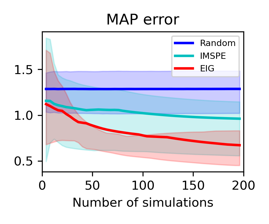
(a) MAP error

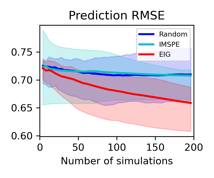
(b) RMSE

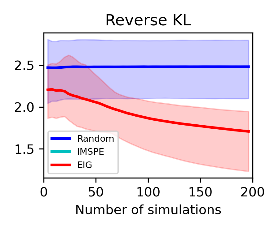
(c) $\mathbb{D}_{\mathrm{KL}}(p_{T}||p_{*})$

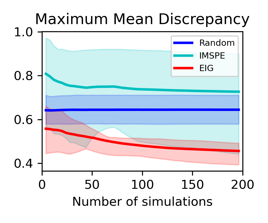
(d) $\operatorname{MMD}(p_{T},p_{*})$

Figure 1: Synthetic experiment results comparing BACON (indicated as EIG) to random search and the IMSPE approach on random functions sampled from a GP prior.

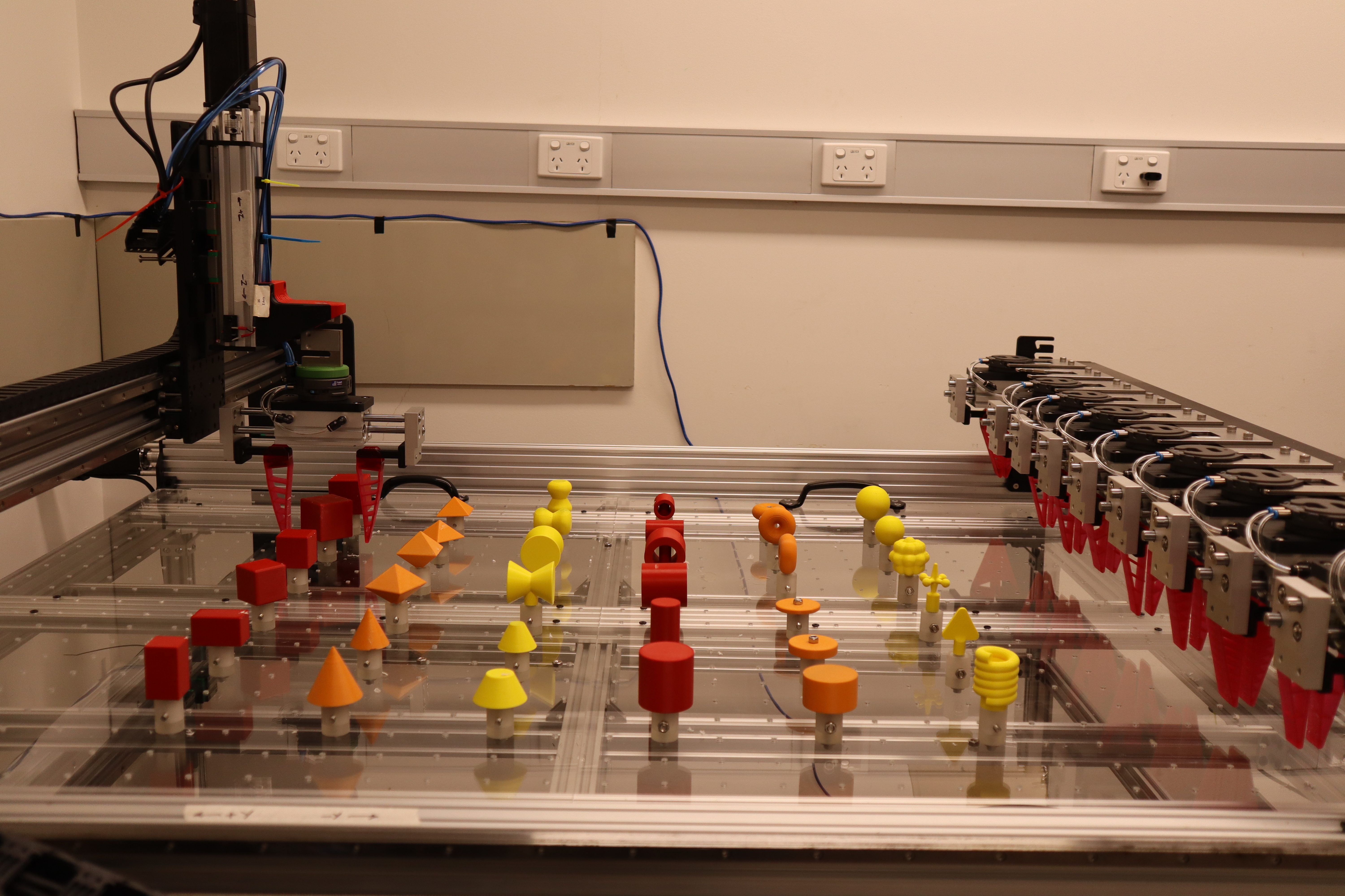
(a)

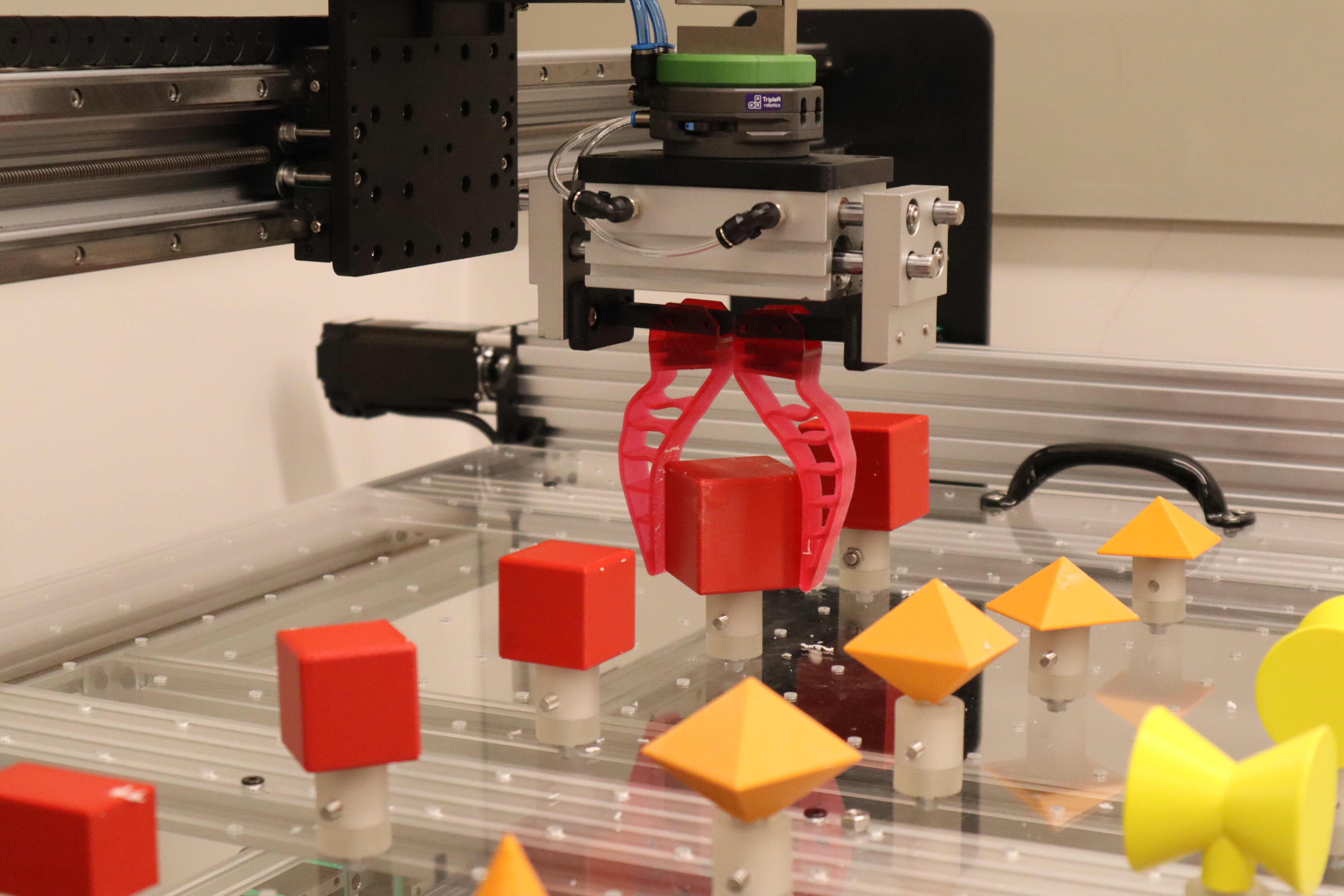
(b)

(c)

Figure 2: Soft-robotics grasping experiment. We calibrate a soft materials simulator against real data from physical grasping from an automated experimentation platform

Performance metrics.

We evaluated each method against a set of performance metrics, which we now describe. The maximum-a-posteriori (MAP) approximation error measures the distance between the mode of the variational distribution and the true parameters ${\boldsymbol{\mathbf{\theta}}}^{*}$. To measure the quality of the learnt model in predicting real outcomes, we also evaluated the root mean square error (RMSE) between the expected GP predictions under the learnt variational distribution and real outcomes: $\mathrm{RMSE}:=\sqrt{\frac{1}{N}\sum_{i=1}^{N}(\mathbb{E}_{q({\boldsymbol{\mathbf{\theta}}})}[\mu({\boldsymbol{\mathbf{x}}}_{i}^{*},{\boldsymbol{\mathbf{\theta}}}^{*};{\boldsymbol{\mathbf{\theta}}})]-y_{i}^{*})^{2}}$, where $y_{i}^{*}=f({\boldsymbol{\mathbf{x}}}_{i}^{*})+\nu_{i}^{*}$ are observations of the true function over a set of designs $\{{\boldsymbol{\mathbf{x}}}_{i}^{*}\}_{i=1}^{N}\subset\mathcal{X}$ placed on a uniform grid the design space.

Information gain.

Lastly, we also evaluated two sample-based estimates of the KL divergence [Szabo14ite]. Namely, $\mathbb{D}_{\mathrm{KL}}(p_{T}||p_{0})$ corresponds to the KL divergence between the final MCMC posterior (given all simulations and real data) and the initial one (given only the real data and an initial set of randomised simulations) both estimated over the learnt GP model. The column $\mathbb{D}_{\mathrm{KL}}(p_{T}||p^{*})$ indicates the KL divergence between the final MCMC posterior $p_{T}$ and the posterior $p_{*}$ with full knowledge of the simulator, which can be cheaply evaluated in this synthetic scenario. The average of $\mathbb{D}_{\mathrm{KL}}(p_{T}||p_{0})$ is an indicator for the expected information gain of an algorithm, given that it is the expected relative entropy across the possible trajectories of observations. Meanwhile $\mathbb{D}_{\mathrm{KL}}(p_{T}||p^{*})$ indicates how far the estimates are from the best possible posterior given the available real data.

	$\mathbb{D}_{\mathrm{KL}}(p_{T}||p_{0})$	$\mathbb{D}_{\mathrm{KL}}(p_{T}||p^{*})$
Random	0.67 $\pm$ 0.36	1.59 $\pm$ 0.51
IMSPE	0.31 $\pm$ 0.18	1.91 $\pm$ 0.49
BACON	0.81 $\pm$ 0.46	1.46 $\pm$ 0.55
VBMC	–	0.94 $\pm$ 0.36

Table 1: Results for 2+2D synthetic problem after $T=50$ iterations (batch of $B=4$). Here $\mathbb{D}_{\mathrm{KL}}(p_{T}||p_{0})$ corresponds to the KL divergence between the final posterior and the starting one (higher is better), while $\mathbb{D}_{\mathrm{KL}}(p_{T}||p_{*})$ is the KL between the final MCMC posterior and the posterior with full knowledge of the simulator $p_{*}$ (lower is better). Averages were over 10 independent runs.

6.1 Baselines

Our algorithmic baselines were chosen to illustrate the main approaches currently available in the literature. Both are employed as adaptive baselines, in the sense that their GP models are updated with the latest observations before proceeding to the next iteration.

Random search.

This baseline samples simulation designs ${\boldsymbol{\mathbf{\hat{{\boldsymbol{\mathbf{x}}}}}}}_{t}\sim\mathcal{U}(\mathcal{X})$ from a uniform distribution over the design space $\mathcal{X}$ and calibration parameters from the prior ${\boldsymbol{\mathbf{\hat{\theta}}}}_{t}\sim p({\boldsymbol{\mathbf{\theta}}}^{*})$.

IMSPE with MAP estimates.

Koermer2023 use an approach that chooses design ${\boldsymbol{\mathbf{\hat{{\boldsymbol{\mathbf{x}}}}}}}_{t}$ and calibration ${\boldsymbol{\mathbf{\hat{\theta}}}}_{t}$ are then chosen by minimising the integrated GP-predicted mean squared error: IMSPE_t(^z) &:= ∫_Z E[