LoRA-Ensemble: Efficient Uncertainty Modelling for Self-attention Networks

Abstract

Numerous crucial tasks in real-world decision-making rely on machine learning algorithms with calibrated uncertainty estimates. However, modern methods often yield overconfident and uncalibrated predictions. Various approaches involve training an ensemble of separate models to quantify the uncertainty related to the model itself, known as epistemic uncertainty. In an explicit implementation, the ensemble approach has high computational cost and high memory requirements. This particular challenge is evident in state-of-the-art neural networks such as transformers, where even a single network is already demanding in terms of compute and memory. Consequently, efforts are made to emulate the ensemble model without actually instantiating separate ensemble members, referred to as implicit ensembling. Here, we introduce LoRA-Ensemble, a parameter-efficient deep ensemble method for self-attention networks, which is based on lora. Initially developed for efficient LLM fine-tuning, we extend LoRA to an implicit ensembling approach. By employing a single pre-trained self-attention network with weights shared across all members, we train member-specific low-rank matrices for the attention projections. Our method exhibits superior calibration compared to explicit ensembles and achieves similar or better accuracy across various prediction tasks and datasets.

1 Introduction

Machine learning models are increasingly applied also in fields where incorrect estimates may have severe consequences, e.g., autonomous driving, medical diagnosis, (extreme) weather event prediction, or agricultural management decision support. In such applications well-calibrated predictive uncertainties are crucial to enable self-diagnosis. Uncertainty can be separated into two components. Aleatoric uncertainty, a.k.a. irreducible noise, is inherent in the data. Epistemic uncertainty on the other hand stems from a lack of knowledge about certain regions of the input space, due to a lack of training data [Der Kiureghian and Ditlevsen, 2009].

Quantification of epistemic uncertainty in large machine learning models is non-trivial. Analytical computation is usually intractable, thus research has focused on efficient approximations [Graves, 2011, Blundell et al., 2015, Welling et al., 2011]. To date, probabilistic ensembles remain the best-performing approach [Lakshminarayanan et al., 2017]. In a naïve implementation, such an ensemble consists of multiple independently trained models. Individual models are interpreted as Monte Carlo samples from the posterior weight space and are used to obtain an unbiased estimator of the posterior distribution. To achieve a low correlation between ensemble members one can capitalize on the stochastic nature of the training process and start from different initial weights, and/or sample different random batches of data. The basic principle is that the predictions of different ensemble members will agree near observed training samples, whereas they may vary far away from the training data. Their spread therefore serves as a measure of epistemic uncertainty. Even small ensembles often capture the uncertainty well (in expectation), i.e., they are well calibrated.

An issue with naïve ensembles is that their computational cost and memory footprint grow proportionally to the number of ensemble members. For smaller models explicit ensembling may still be feasible, albeit with higher financial cost and energy consumption. For modern neural networks with up to several billion parameters, hardware restrictions render the naïve approach intractable, in particular, one can no longer hold the entire ensemble in memory. Consequently, a lot of research has gone into ways of creating ensembles implicitly, without requiring multiple copies of the full base model [Wen et al., 2020, Wenzel et al., 2020, Huang et al., 2017, Turkoglu et al., 2022]. Unfortunately, most of these parameter-efficient ensembling techniques are not applicable to the newest generation of neural networks. Transformer networks [Vaswani et al., 2017] have recently become popular due to their superior ability to capture complex structures in data. However, implicit ensembling schemes tend to underperform for transformers or are entirely incompatible with them.

Several studies have shown that modern neural networks are heavily overparametrized and that their results have low intrinsic dimension [Li et al., 2018a, Aghajanyan et al., 2020]. This led Hu et al. [2021] to propose lora as a way of deploying individually fine-tuned llm to different tasks while avoiding the prohibitively large memory and compute requirements of retraining them. It turns out that the weight matrices in such models can be factorized to have very low rank, with hardly any loss in prediction performance.

This led us to use lora as the basis for a novel, parameter-efficient ensemble method that is tailored to the transformer architecture. In line with the trend towards transfer learning, our method uses a pre-trained transformer model, which is expanded into an implicit ensemble by varying the lora factorization, while keeping the backbone weights frozen. In this way, our method only requires a small number of additional parameters to turn an existing transformer model into a diverse ensemble whose performance across various tasks is comparable to an Explicit Ensemble. In summary, our contributions are:

• We introduce lora-Ensemble, a parameter-efficient probabilistic ensemble method for self-attention networks.

• lora-Ensemble can be readily combined with most pre-trained transformer networks, irrespective of their specific architecture and application domain: it simply replaces the linear projection layers in the attention module with lora-Ensemble layers.

• We apply lora-Ensemble to different classification tasks including: conventional image labeling, classification of skin lesions in dermatoscopic images, and sound classification from spectrograms. In these experiments, lora-Ensemble not only consistently outperforms other implicit ensemble schemes but also, surprisingly, its classification accuracy and uncertainty calibration are often even better than that of an Explicit Ensemble.

2 LoRA-Ensemble

The lora technique makes it possible to use a pre-trained model and fine-tune it without having to retrain all its parameters. This is particularly beneficial for modern neural networks with large parameter spaces. The underlying principle is to freeze the pre-trained model weights $W_{0}\in\mathbb{R}^{k\times d}$ and instead constrain the updates to a low-rank decomposition. This can be expressed mathematically as:

$$W=W_{0}+\Delta W=W_{0}+B\!\cdot\!A\;.$$ (1)

Here $B\in\mathbb{R}^{k\times r}$ and $A\in\mathbb{R}^{r\times d}$ are two trainable low-rank matrices, where $r\ll\min(d,k)$. $W$ and $\Delta W$ are then multiplied with the same input $x$, which yields the following modified forward pass:

$$h=W_{0}\cdot x+\Delta W\cdot x=W_{0}\cdot x+B\!\cdot\!A\cdot x\;.$$ (2)

lora applies this low-rank updating scheme only to weights in the self-attention modules of a transformer model while leaving the interleaved MLP modules untouched. I.e., the weight matrices being updated are $W_{q}$, $W_{k}$, and $W_{v}$ for the query, key, and value of the attention mechanism, as well as the $W_{o}$ for merging the multi-head outputs. The former three are each treated as a single matrix, disregarding the fact that they are typically sliced into multiple attention heads. [Hu et al., 2021]

Although not designed with uncertainty calibration in mind, the lora concept fulfills all the requirements of an implicit deep ensemble: By modifying the weights of the highly nonlinear self-attention mechanism one is able to generate a diverse collection of networks with the same architecture and objective. By learning an additive, low-rank update $\Delta W=B\!\cdot\!A$ rather than directly tuning the weight matrices, the expansion into a model ensemble adds only a small number of parameters and is efficient. In detail, we start from a single, pre-trained model with frozen parameters $W_{0}$ and expand it with a set of trainable low-rank matrices $\Delta W_{i}$, $\forall i=1\ldots N$. At each transformer block, there now is a different forward pass per ensemble member $i$, as illustrated in Fig. 1:

$$h_{i}=W_{0}\cdot x+\Delta W_{i}\cdot x=W_{0}\cdot x+B_{i}\!\cdot\!A_{i}\cdot x\;,$$ (3)

leading to $N$ different predictions $T_{\theta_{i}}(X)$ for a given input $X$. From those individual predictions, we compute the ensemble estimate by simple averaging:

$$\mathbb{E}[Y|X]=\frac{1}{N}\sum_{i=1}^{N}T_{\theta_{i}}(X)\;.$$ (4)

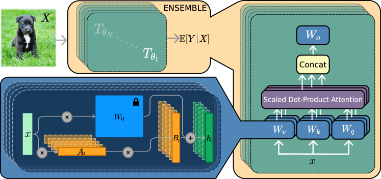
Figure 1: A schema of a lora-Ensemble. The computation structure of the multi-head self-attention module (right), and lora-Ensemble module (bottom left). $X$ denotes the actual input, and $x$ represents the intermediate input representation.

2.1 Implementation

In practice, our lora-Ensemble is implemented by replacing the respective linear layers ($W_{q}$, $W_{k}$, $W_{v}$, and $W_{o}$) in the pre-trained model architecture with custom lora modules.

As a backbone for experiments with image datasets, we employ a vit model [Dosovitskiy et al., 2020]. The chosen architecture is the base variant with patch size $32\times 32$ as defined in Dosovitskiy et al. [2020]. We load the weights from torchvision, which were trained on ImageNet-1k [Deng et al., 2009], using a variant of the training recipe from Touvron et al. [2020], for details refer to their documentation.

The forward pass through the backbone is parallelized by replicating the input along the batch dimension. In each lora module, the data is split into separate inputs per member and passed to the respective member with the help of a vectorized map, which allows a parallelized forward pass even through the lora modules. The outputs are then again stacked along the batch dimension. In this way, one makes efficient use of the parallelization on gpu, while at the same time avoiding loading the pre-trained backbone into memory multiple times.

As a backbone for audio experiments, we use the ast backbone [Gong et al., 2021]. That architecture was inspired by vit (more specifically the data-efficient version of vit akin to deit [Touvron et al., 2020]) but is designed specifically for audio spectrograms. Following Gong et al. [2021], we initialize the audio model weights by transferring and appropriately interpolating them from ImageNet pre-training. See Appendix F and G for details. As the ast version of lora-Ensemble would run into memory limits, we introduce chunking. While the forward pass through the backbone is still parallelized, the lora modules are called sequentially.

Finally, the pre-trained model does not have the correct output dimension for our prediction tasks (i.e., it was trained for a different number of classes). Therefore we entirely discard its last layer and add a new one with the correct dimensions, which we train from scratch. Obviously, the weights of that last layer are different for every ensemble member. We parallelize it in the same way as the lora module described above.

We publicly release a PyTorch implementation of lora-Ensemble, as well as pre-trained weights to reproduce the experiments, on GitHub.

3 Experiments

In the following section, we evaluate the proposed lora-Ensemble on several datasets with regard to its predictive accuracy, uncertainty calibration, and memory usage. For each experiment we also show 1-sigma error bars, estimated from five independent runs with different random initializations.

As a first sandbox experiment, we perform image classification for the popular, widely used CIFAR-100 benchmark [Krizhevsky, 2009]. The dataset consists of 100 object classes, each with 600 samples, for a total size of 60 000 images. From that set, 10 000 images are designated test data, with all classes equally distributed between the training and testing portions.

The HAM10000 dataset was proposed for the Human Against Machine with 10 000 training images study [Tschandl et al., 2018]. It consists of 10 015 dermatoscopic images of pigmented skin lesions, collected from different populations. The dataset was initially assembled to compare machine learning methods against medical professionals on the task of classifying common pigmented skin lesions. Compared to CIFAR-100, this is arguably the more relevant test bed for our method: in the medical domain, uncertainty calibration is critical, due to the potentially far-reaching consequences of incorrect diagnoses and treatment planning.

For both datasets, lora-Ensemble is compared against several baselines. As a sanity check, we always include results obtained with a single vit model, as well as with a single vit model with lora in the attention modules. These models do not have a dedicated mechanism for uncertainty calibration, instead, the predicted class-conditional likelihoods are used to quantify uncertainty. Furthermore, we compare to an explicit model ensemble, and mcdropout as implemented in Li et al. [2023]. The lora rank was empirically set to 8 for CIFAR-100 and 4 for HAM10000.

For each method, we evaluate both the classification accuracy (percentage of correctly classified test samples) and the ece [ECE, Guo et al., 2017]. The latter measures the deviation from a perfectly calibrated model, i.e., one where the estimated uncertainty of the maximum-likelihood class correctly predicts the likelihood of a miss-classification. For more evaluation metrics refer to Appendix A.

As a further benchmark from a different application domain, we process the ESC-50 environmental sounds dataset [Piczak, 2015]. It consists of 2000 sound samples, each five seconds long, that represent 50 different semantic classes with 40 samples each. To prepare the raw input waveforms for analysis, they are converted into 2-dimensional time/frequency spectrograms, see Gong et al. [2021]. These spectrograms form the input for the ast, a state-of-the-art transformer model for sound classification.

As for the vit model, we train an ast version of lora-Ensemble by modifying the attention weights with different sets of lora weights. That ensemble is then compared to a single instance of ast with and without lora, to an Explicit Ensemble of ast-models, and to an mcdropout variant of ast, similar to Li et al. [2023]. For ESC-50 a lora rank of 16 worked best, presumably due to the larger domain gap between (image-based) pre-training and the actual audio classification task. The experimental evaluation in Gong et al. [2021] employs the same performance metrics as before, but a slightly different evaluation protocol. Model training (and evaluation) is done in a 5-fold cross-validation setting, where the epoch with the best average accuracy across all five folds is chosen as the final model. The performance metrics given below are calculated by taking the predictions of all five folds at the chosen epoch and evaluating accuracy and ece jointly. While the accuracy calculated this way is equivalent to the average of all five folds, ece is not, so this method results in a more realistic calculation of the calibration metric.

3.1 Computational Cost

In addition to evaluating classification performance and calibration, we assess the computational cost in terms of parameters, training, and inference time. The required resources are presented in Tab. 1.

Table 1: Parameter counts and computation times for an Explicit Ensemble of 16 ViT models and the corresponding LoRA-Ensemble. Training time is the average duration for one epoch on CIFAR-100, with batch size 32. Inference time is the average duration of a forward pass, with batch size 1.

Method	Parameter overhead	Training time [s]	Inference time [ms]
Explicit Ensemble	$16\times 87\mathrm{M}$	$16\times 139$	$16\times 4.6$
lora-Ensemble	$1.12\times 87\mathrm{M}$	1108	22.7

The total number of parameters is reported for an ensemble of 16 members, and matrices $A$ and $B$ with rank 8 when using lora. Choosing a different rank will slightly alter the parameter count. In many cases a lower rank may suffice, cf. Hu et al. [2021]. All times were measured on a single NVIDIA Tesla A100-80GB GPU. Training time is given as the average wall clock time per training epoch on CIFAR-100, with 16 ensemble members. Inference time is computed as the average time for a single forward pass for a CIFAR-100 example, with batch size 1. As mentioned in Sec. 2.1, the forward pass for the Explicit Ensemble processes the members sequentially. Hence, we calculate the average time needed for one member and multiply it by 16. It is evident that the proposed method uses significantly fewer parameters and less memory. lora-Ensemble also trains faster, and speeds up inference more than 3 times.

We point out that, with our current implementation, the runtime comparisons are still indicative. It turns out that PyTorch’s vectorized map (vmap) has a large one-time overhead that is only amortized when using large ensembles, while small ensembles are slowed down. Practical ensemble sizes will benefit when implemented in a framework that supports just-in-time compilation, like JAX.

3.2 CIFAR-100

Our two target metrics, classification accuracy and ece are both graphed against ensemble size in Fig. 2. Quantitative results for all compared methods are summarized in Tab. 2.

lora-Ensemble consistently reaches higher accuracy than mcdropout, with a notable edge of approximately 5 percentage points for ensembles of four or more members. Surprisingly, it also consistently surpasses the Explicit Ensemble by about 2 percentage points, apparently a consequence of the fact that already a single vit model, and thus every ensemble member, benefits from the addition of lora.

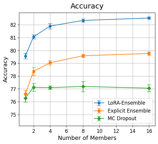
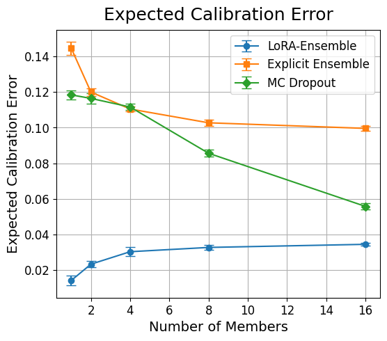
Figure 2: Accuracy and ece on CIFAR-100, with different ensemble sizes.

With lora-Ensemble also the estimates of predictive uncertainty are better calibrated. Interestingly, the calibration is already very good at small ensemble sizes but slightly degrades when adding more members. The reliability diagram in Fig. 3 somewhat elucidates this unexpected behavior. It turns out that lora-Ensemble is generally under-confident, meaning that the classification is more accurate than the model suggests. Rahaman and Thiery [2020] have found that when ensembling under-confident models, the accuracy grows faster than the confidence. As a result, the difference between accuracy and confidence tends to grow, worsening calibration metrics. Note that in safety-critical applications under-confident models that over-estimate the uncertainty are often preferable to over-confident ones.

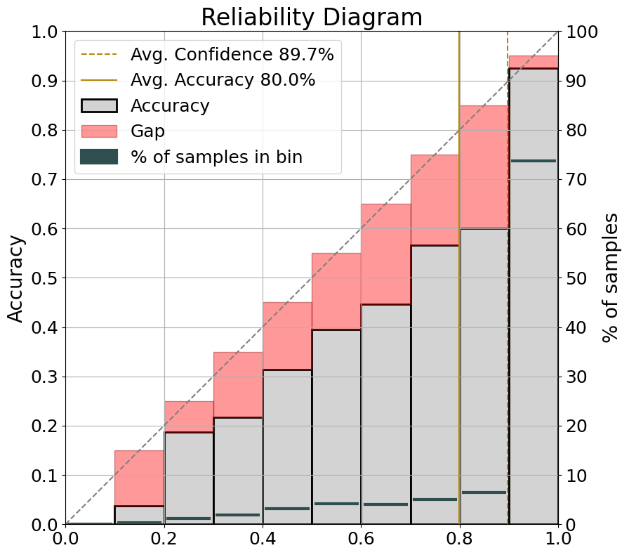
Figure 3: Reliability diagrams for Explicit Ensemble (left) and lora-Ensemble (right) with 16 members, on CIFAR-100.

mcdropout is not well calibrated for smaller ensembles, but progressively catches up as the ensemble size increases. We note that, at least for the specific dataset and architecture, both implicit ensembling methods improve over the Explicit Ensemble that is commonly regarded as the gold standard. Notably, just adding lora to a single model without any ensembling already improves calibration beyond that of a 16-member Explicit Ensemble. This effect can possibly be linked to the well-documented over-parametrization of modern neural networks. It has been shown that their massively inflated parameter space tends to attain higher predictive accuracy at the cost of worse calibration [e.g., Guo et al., 2017]. Adding lora, but treating all pre-trained weights as constants greatly shrinks the trainable parameter space and could thereby favor calibration.

3.3 HAM10000 Lesion Classification

In many medical applications, well-calibrated models are essential. As a test case, we use the classification of pigmented skin lesions and again compare the same group of models in terms of accuracy and calibration. The results are summarized in Tab. 2, and further evaluation metrics can be found in Appendix A.3, Tab. 6.

Similar to the CIFAR-100 evaluation, lora-Ensemble outperforms all other methods by a clear margin, with respect to both classification accuracy and calibration. The experiments also further support the above discussion of confidence vs. ensemble size (Sec. 3.2). For HAM10000 lora-Ensemble is slightly over-confident (just like the Explicit Ensemble) and, indeed, its calibration error decreases with ensemble size in this case.

Table 2: Model performance on the CIFAR-100 and HAM10000 datasets for the compared methods. Ensembles have 16 members. Best score for each metric in bold, second-best underlined.

	CIFAR-100		HAM1000
Method	Accuracy ($\uparrow$)	ECE ($\downarrow$)	Accuracy ($\uparrow$)	ECE ($\downarrow$)
Single Network	$76.6\pm 0.3$	$0.145\pm 0.004$	$84.1\pm 0.3$	$0.139\pm 0.004$
Single Network with LoRA	$79.6\pm 0.2$	$\textbf{0.014}\pm 0.003$	$83.2\pm 0.7$	$\underline{0.085}\pm 0.004$
MC Dropout	$77.1\pm 0.5$	$0.055\pm 0.002$	$83.7\pm 0.4$	$0.099\pm 0.007$
Explicit Ensemble	$\underline{79.8}\pm 0.1$	$0.100\pm 0.001$	$\underline{85.8}\pm 0.2$	$0.105\pm 0.002$
LoRA-Ensemble	$\textbf{82.5}\pm 0.1$	$\underline{0.035}\pm 0.001$	$\textbf{88.0}\pm 0.2$	$\textbf{0.037}\pm 0.002$

3.4 ESC-50 Environmental Sound Classification

To go beyond computer vision tasks, lora-Ensemble is also applied to an audio dataset, using the ast as the backbone model. Performance is again evaluated in terms of accuracy and ece. The results are summarized in Tab. 3.

Table 3: Model performance on the ESC-50 dataset for the compared methods. Ensembles have 8 members due to memory limitations. Best score for each metric in bold, second-best underlined.

Method	Accuracy ($\uparrow$)	ECE ($\downarrow$)
Single Network	$89.3\pm 0.7$	$0.040\pm 0.005$
Single Network with LoRA	$88.1\pm 0.1$	$0.039\pm 0.002$
MC Dropout	$89.4\pm 0.3$	$0.087\pm 0.003$
Explicit Ensemble	$\textbf{91.3}\pm 0.3$	$\underline{0.026}\pm 0.003$
LoRA-Ensemble	$\underline{91.0}\pm 0.2$	$\textbf{0.022}\pm 0.003$

On this dataset lora-Ensemble does not significantly outperform the Explicit Ensemble, but still matches its performance with much lower computational demands, see Appendix I. Accuracy is insignificantly lower, whereas calibration is slightly better. We note that, remarkably, the weights used in the transformer modules and for creating patch embeddings were pre-trained on images rather than audio streams.

3.5 Sensitivity Analysis: LoRA Rank

The main hyper-parameter introduced by adding lora is the rank of the low-rank decomposition (i.e., the common dimension of the matrices $A$ and $B$). Varying that rank modulates the complexity of the model for the learning task. We have empirically studied the relationship between rank, accuracy, and ece. Here we show results for the HAM10000 dataset, additional results for CIFAR-100 can be found in Appendix B.

On HAM10000 we observe a clear trade-off between accuracy and calibration, Fig. 4. With increasing rank the classification accuracy increases while the calibration deteriorates, in other words, one can to some degree balance predictive accuracy against uncertainty calibration by choosing the rank. The trend is again in line with our previous observations about over-confident models.

Figure 4: Impact of lora rank on accuracy and ece, for the HAM10000 dataset.

Our focus in this work is on model calibration. We therefore generally choose the rank to favor calibration, even at the cost of slightly lower classification accuracy.

4 Related Work

4.1 Estimation of Epistemic Uncertainty

A lot of work has gone into estimating the epistemic uncertainty in ann. As the analytical computation of the posterior in such models is generally intractable, methods for approximate Bayesian inference have been proposed. Such methods rely on imposing an appropriate prior on the weights and using the likelihood of the training data to get an approximate posterior of the weight space.

The main techniques are, on the one hand, Variational Inference [Graves, 2011, Ranganath et al., 2014], which Blundell et al. [2015] have specialized to neural networks as Bayes by Backprop. And on the other hand variants of mcmc [Neal, 1996, Chen et al., 2014], including sgld [Welling et al., 2011]. These, however, are often not able to accurately capture high-dimensional and highly non-convex loss landscapes, like the ones usually encountered in deep learning [Gustafsson et al., 2019].

4.2 Ensembles and Implicit Ensembling

Lakshminarayanan et al. [2017] have proposed a method known as deep ensembles. It uses a set of neural networks with identical architecture that are independently and randomly initialized, and (as usual) trained with variants of sgd. While the latter introduces further stochasticity, Fort et al. [2019] have shown that the initialization of the weights is more important to explore the admissible weight space. Ensemble members will generally converge to different modes of the loss function, such that they can be considered Monte Carlo samples of the posterior distribution [Wilson and Izmailov, 2020, Izmailov et al., 2021]. While ensembles, in general, yield the best results in terms of accuracy and uncertainty calibration, a straightforward implementation suffers from high memory and compute requirements, since multiple instances of the full neural network must be trained and stored. This can become prohibitive for modern neural networks with many millions, or even billions, of parameters.

Consequently, researchers have attempted to find ways of mimicking the principle of deep ensembles without creating several full copies of the base model. Gal and Ghahramani [2015] have proposed mcdropout, where the posterior is approximated by sampling different dropout patterns at inference time. While this is less expensive in terms of memory, performance is often worse. Masksembles [Durasov et al., 2020] are a variant that attempts to select suitable dropout masks in order to obtain better uncertainty estimates. Snapshot Ensembles [Huang et al., 2017] use cyclic learning rates to steer the learning process such that it passes through multiple local minima, which are then stored as ensemble members. This reduces the training effort but does not address memory requirements or inference time.

Particularly relevant for our work are attempts that employ a shared backbone and modify only selected layers. Havasi et al. [2020] follow that strategy, in their case only the first and last layer of a neural network are replicated and trained independently to emulate an ensemble. BatchEnsemble [Wen et al., 2020] is similar to lora-Ensemble in that it also uses low-rank matrices to change the model parameters. More specifically, shared weight matrices are modulated by element-wise multiplication with different rank-1 matrices to achieve the behavior of a deep ensemble while adding only a small number of parameters. Wenzel et al. [2020] take this concept further by also ensembling over different hyper-parameter settings. Turkoglu et al. [2022] freeze all weights of the base model and instead vary the feature-wise linear modulation [FiLM, Li et al., 2018b, Takeda et al., 2021].

A related concept was recently introduced for llm: the Mixtral of Experts model [Jiang et al., 2024] averages over a sparse mixture of experts to efficiently generate text.

4.3 Low-Rank Adaptation in Transformer Networks

lora was originally conceived as a parameter-efficient way of fine-tuning llm [Hu et al., 2021]. It is based on the observation that, while modern neural networks have huge parameter spaces, the solutions they converge to have much lower intrinsic dimension [Li et al., 2018b, Aghajanyan et al., 2020]. lora exploits this and Hu et al. [2021] show that even when fine-tuning only a low-rank update matrix $B\!\cdot\!A$ (sometimes with rank as low as one or two), the resulting models are competitive with much more expensive fine-tuning schemes. The method quickly became popular and has since also been extended with weight-decomposition [Liu et al., 2024]. The lora idea has been applied in various fields, notably for denoising diffusion models [Luo et al., 2023, Golnari, 2023].

As we have shown, lora’s adaptation technique naturally lends itself to parameter-efficient ensembling. We study the resulting ensemble for uncertainty calibration, a similar approach has concurrently been explored for the purpose of fine-tuning large language models [Wang et al., 2023], with promising results.

5 Limitations & Future Work

We propose a parameter-efficient ensembling method, which performs well in the conducted experiments. These results, however, still only heuristically show the power of the method, as there is no theoretical proof, that the members do, in fact, converge to different modes and therefore yield sufficient diversity to fully capture the underlying statistics. The presented work also leaves a number of questions that are yet to be answered. In our experiments, we did not evaluate lora-Ensemble on very large datasets, such as those often found in natural language processing. It would be interesting to see, how the method performs on such datasets. Correspondingly, it would also be useful to explore how lora-Ensemble performs on llm, especially as these models become ever more popular. Additionally, while our method does address the restrictive memory usage of traditional ensembles, it does not reduce computational complexity. The data still needs to be passed through the model once per batch. Furthermore, it is theoretically possible to perform approximate inference on the parameter distribution of the lora matrices. This would enable drawing an infinite number of ensemble members from the approximate posterior.

As discussed by Rahaman and Thiery [2020], our work also suggests that in a high-parameter regime, deep ensembles may not exhibit the same behavior as they do in a low-parameter regime, where they typically improve calibration properties. We have previously witnessed this type of phase shift in bias-variance trade-off for large neural networks akin to Double Descent Phenomena [Nakkiran et al., 2021]. It would be valuable to conduct an in-depth analysis of deep ensemble behavior in high-parameter regimes, while also considering data size and compute.

6 Conclusion

We have presented lora-Ensemble, a novel, parameter-efficient method for probabilistic learning that is tailored to the transformer architecture (and potentially other architectures that make use of the attention mechanism). lora-Ensemble uses a simple, but efficient trick to turn a single base model into an implicit ensemble: the weights of the base model are kept frozen, but are modulated with the lora mechanism. By training multiple, stochastically varying instances of the low-rank matrices that define the modulation, one obtains a diverse set of ensemble members that share the majority of their weights (specifically, those of the base model) and introduces only minimal overhead through the coefficients of their individual low-rank matrices. Our experiments on two different computer vision tasks and a sound classification task show that the proposed approach can outperform other, implicit as well as explicit, ensembling strategies in terms of both classification performance and uncertainty calibration.

Broader Impact

In recent years, the size of machine learning models has expanded rapidly. GPT-3 [Brown et al., 2020] has 175 billion parameters, while its successor, GPT-4, is rumored to contain over 1.7 trillion parameters, with training costs exceeding $100 million. As the trend toward larger models continues, growing computational resources are required. With this work, lora-Ensemble aims to contribute to more efficient ensemble methods, considering the resource usage and environmental impact of AI models. This effort strives for more sustainable practices, advancing the concept of "Green AI."

Appendix A More Experiments & Results

This section presents additional experimental results, including a new dataset: CIFAR-10, a new accuracy metric: F1 score, and new calibration metrics: NLL (Negative Log-Likelihood) and Brier score. For the definition of metrics refer to Appendix K.

A.1 CIFAR-10

The results for the CIFAR-10 dataset, as shown in Tab. 4, indicate that lora-Ensemble outperforms all other methods across all metrics. Following closely is a single network enhanced with lora. This mirrors the results found in the main paper for CIFAR-100, with the exception of the calibration for a single model. It is important to note that although all methods achieve high accuracy and the differences between them are minimal, calibration is nearly perfect for most approaches. This suggests that the CIFAR-10 dataset is relatively easy for modern transformer models, and the results should not be over-interpreted. Nevertheless, the consistent performance across different random seeds suggests that the ranking is likely significant. Given the balanced nature of the CIFAR-10 dataset, the accuracy and F1-score are almost identical.

Table 4: Performance on the CIFAR-10 dataset for all compared methods. Ensembles have 16 members. Best score for each metric in bold, second-best underlined.

Method	Accuracy ($\uparrow$)	F1 ($\uparrow$)	ECE ($\downarrow$)	NLL ($\downarrow$)	Brier ($\downarrow$)
Single Net	$92.8\pm 0.1$	$92.8\pm 0.1$	$0.051\pm 0.001$	$0.333\pm 0.003$	$0.120\pm 0.002$
Single Net w/ LoRA	$\underline{94.5}\pm 0.0$	$\underline{94.5}\pm 0.0$	$\underline{0.009}\pm 0.001$	$\underline{0.163}\pm 0.002$	$\underline{0.082}\pm 0.001$
MC Dropout	$92.9\pm 0.2$	$92.9\pm 0.2$	$0.023\pm 0.002$	$0.260\pm 0.005$	$0.110\pm 0.003$
Explicit Ensemble	$94.1\pm 0.1$	$94.1\pm 0.1$	$0.031\pm 0.001$	$0.181\pm 0.002$	$0.087\pm 0.001$
LoRA-Ensemble	$\textbf{95.9}\pm 0.1$	$\textbf{95.9}\pm 0.1$	$\textbf{0.003}\pm 0.001$	$\textbf{0.128}\pm 0.001$	$\textbf{0.064}\pm 0.000$

A.2 CIFAR-100

The results for the CIFAR-100 dataset are summarized in Tab. 5. lora-Ensemble once again outperforms all other methods in most metrics, except for the calibration error of a single lora-augmented model. The Explicit Ensemble ranks second in terms of accuracy, F1 score, and Brier score. Similar to CIFAR-10, the balanced nature of the CIFAR-100 dataset results in nearly identical accuracy and F1 score.

Table 5: Additional performance metrics on the CIFAR-100 dataset for all compared methods. Ensembles have 16 members. Best score for each metric in bold, second-best underlined.

Method	Accuracy ($\uparrow$)	F1 ($\uparrow$)	ECE ($\downarrow$)	NLL ($\downarrow$)	Brier ($\downarrow$)
Single Net	$76.6\pm 0.3$	$76.6\pm 0.3$	$0.145\pm 0.004$	$1.181\pm 0.019$	$0.370\pm 0.004$
Single Net w/ LoRA	$79.6\pm 0.2$	$79.4\pm 0.2$	$\textbf{0.014}\pm 0.003$	$\underline{0.671}\pm 0.005$	$0.286\pm 0.003$
MC Dropout	$77.1\pm 0.5$	$77.2\pm 0.4$	$0.055\pm 0.002$	$1.138\pm 0.014$	$0.336\pm 0.005$
Explicit Ensemble	$\underline{79.8}\pm 0.1$	$\underline{79.8}\pm 0.2$	$0.100\pm 0.001$	$0.745\pm 0.003$	$\underline{0.284}\pm 0.002$
LoRA-Ensemble	$\textbf{82.5}\pm 0.1$	$\textbf{82.5}\pm 0.1$	$\underline{0.035}\pm 0.001$	$\textbf{0.587}\pm 0.001$	$\textbf{0.253}\pm 0.000$

A.3 HAM10000

Supplementary statistics for HAM10000, along with those presented in the main paper, are provided in Tab. 6. lora-Ensemble achieves the best performance across all metrics. The Explicit Ensemble consistently ranks second, except for calibration, where both a single lora-augmented model and MC Dropout exhibit lower errors.

Table 6: Additional performance metrics on the HAM10000 dataset for all compared methods. Ensembles have 16 members. Best score for each metric in bold, second-best underlined.

Method	Accuracy ($\uparrow$)	F1 ($\uparrow$)	ECE ($\downarrow$)	NLL($\downarrow$)	Brier ($\downarrow$)
Single Net	$84.1\pm 0.3$	$71.4\pm 0.7$	$0.139\pm 0.004$	$1.138\pm 0.040$	$0.291\pm 0.009$
Single Net w/ LoRA	$83.2\pm 0.7$	$70.7\pm 1.3$	$\underline{0.085}\pm 0.004$	$0.569\pm 0.027$	$0.256\pm 0.011$
MC Dropout	$83.7\pm 0.4$	$71.0\pm 0.9$	$0.099\pm 0.007$	$0.631\pm 0.023$	$0.270\pm 0.009$
Explicit Ensemble	$\underline{85.8}\pm 0.2$	$\underline{74.6}\pm 0.4$	$0.105\pm 0.002$	$\underline{0.536}\pm 0.007$	$\underline{0.218}\pm 0.002$
LoRA-Ensemble	$\textbf{88.0}\pm 0.2$	$\textbf{78.3}\pm 0.6$	$\textbf{0.037}\pm 0.002$	$\textbf{0.342}\pm 0.003$	$\textbf{0.175}\pm 0.002$

Appendix B More Sensitivity Analysis: LoRA Rank

As discussed in the paper, varying the rank of the low-rank decomposition in lora allows for modulation of the model size. We investigated the effect of rank on predictive accuracy and uncertainty calibration for lora-Ensemble. The results for the HAM10000 dataset are presented in the main paper, Sec. 3.5. For the CIFAR-100 dataset, our evaluation of lora-Ensemble shows both increased accuracy and improved calibration with increasing rank within the studied range. These findings are illustrated in Fig. 5.

Figure 5: Impact of lora rank on accuracy and ECE, for the CIFAR100 dataset.

This observation aligns with the findings of Rahaman and Thiery [2020], as lora-Ensemble continues to exhibit under-confidence even at higher ranks. Increasing model complexity enhances confidence, thereby improving calibration. However, at rank 32, the calibration of a single network augmented with lora begins to deteriorate, suggesting that a critical boundary has been reached. Beyond this point, the parameter space becomes insufficiently constrained, leading to effects similar to those observed by Guo et al. [2017].

At higher ranks, accuracy plateaus while memory demand increases linearly with $\mathcal{O}(d)$ and $\mathcal{O}(k)$ for $A\in\mathbb{R}^{r\times d}$ and $B\in\mathbb{R}^{k\times r}$ respectively, where $d$ and $k$ are the dimensions of the pre-trained weight matrix $W_{0}\in\mathbb{R}^{k\times d}$. Consequently, we selected rank 8 for our CIFAR-100 experiments.

Appendix C Training Details

The CIFAR-10/100 and HAM10000 dataset experiments are based on the ViT-Base-32 architecture [Dosovitskiy et al., 2020]. This model has 12 layers and uses 768-dimensional patch embeddings, and the multi-head attention modules have 12 heads. All vit models for image classification are trained using the AdamW optimizer [Loshchilov and Hutter, 2017]. The base learning rate is initially set to 0.0001. The training uses a learning rate warm-up of 500 steps, where the learning rate increases linearly from 0 to the base learning rate before switching to a cosine decline over the rest of the steps. During the experiments, the gradients were calculated and then clipped not to exceed a maximum norm of 1. In the case of HAM10000, we used a weighted cross entropy loss that considered the estimated effective number of samples, which was determined using a beta parameter of 0.9991 [Cui et al., 2019]. Uniform class weights were used for all other datasets. The maximum number of training epochs varies depending on the dataset. For CIFAR-100, the model is trained for 16 epochs (just over 25000 steps), while on HAM10000, it is trained for 65 epochs. Overall, the hyperparameters used in this work were loosely based on Conrad [2023]. The models were trained using pre-trained weights from torchvision 0.17.1 on an NVIDIA Tesla A100 graphics card. Moreover, the lora models were configured with a rank of 8 for both CIFAR-10 and CIFAR-100 and a rank of 4 for HAM10000. For Monte Carlo Dropout the dropout rate was empirically set to be $0.2$. Refer to Appendix J for details.

The settings used for the ESC-50 dataset training are similar to those used in Gong et al. [2021]. However, we used a batch size of 1 instead of 48 to enable training on a single GPU. The base learning rate is set to 0.00001 for the Explicit Ensemble as well as MC Dropout experiments and 0.00005 for lora-Ensemble. These learning rates are lower than the ones used in Gong et al. [2021], which is due to the smaller batch size. Refer to the Appendix H for more details. The lora models were implemented with a rank of 16. The dropout rate for MC dropout was kept at $0.2$.

As Fort et al. [2019] have shown, varying initializations of the weights are most important to getting diverse ensemble members. For this reason, various initialization methods and corresponding parameters were tried, with a Xavier uniform initialization [Glorot and Bengio, 2010] with gain 10, giving the best combination of accuracy and calibration. For more information, refer to Appendix D. This setting is kept for models across all datasets, including the one with an ast backbone.

For the same reason, we investigated whether adding noise to the pre-trained parameters of an Explicit Ensemble increases its performance through a higher diversity of members. However, the results did not show any additional benefits beyond what the randomly initialized last layer already provided. Therefore, it was not utilized. For more details, refer to Appendix E.

Appendix D Initialization of LoRA-Ensemble Parameters

Randomness in initialization is a key driver of diversity among ensemble members [Fort et al., 2019]. Therefore, finding the right balance between diversity and overly disrupting parameters is crucial. Hu et al. [2021] propose using a random Gaussian initialization for $A$ while setting $B$ to zero. This approach results in $\Delta W=BA$ being zero at the start of training. In our experiments, we adopt this pattern by always initializing $B$ to zero while varying the parameters and methods for initializing $A$. Following the method outlined by Hu et al. [2021], our initial experiments concentrated on the Gaussian initialization of $A$, with a mean $\mu=0$ and varying standard deviations. Additionally, we tested the Xavier uniform initialization [Glorot and Bengio, 2010] using different values for the gain. All tests were conducted on the CIFAR-100 dataset and subsequently applied to other experiments. We compared results in terms of accuracy and ece.

Table 7: Accuracy and ece for different initialization methods and varying distribution parameters for LoRA-Ensemble.

Init. Type	Std. / Gain	Accuracy ($\uparrow$)	ECE ($\downarrow$)
Gaussian	0.02	81.2	0.041
	0.05	81.4	0.037
	0.1	81.7	0.035
	0.2	82.1	0.034
	0.5	82.6	0.036
	1	82.5	0.039
	2	81.7	0.046
Xavier Uniform	1	81.5	0.039
	5	82.2	0.034
	10	82.4	0.034
	15	82.6	0.037
	20	82.4	0.038
	30	82.2	0.043

In Tab. 7, the results are quantitatively presented. It is immediately evident that both techniques and all tested parameters perform similarly. While more specialized models may surpass our results in terms of accuracy, our primary focus is on calibration, with the goal of maintaining comparable predictive performance. Visual inspection of the results in Fig. 6 confirms the high similarity among all results. Choosing a small calibration error while maintaining high accuracy as a decision criterion, both Gaussian initialization with a standard deviation of $0.5$ and Xavier uniform initialization with a gain of $10$ or $15$ are viable candidates. Since a gain of $10$ combines high accuracy with the lowest ece, we select Xavier uniform initialization with a gain of $10$ for our experiments.

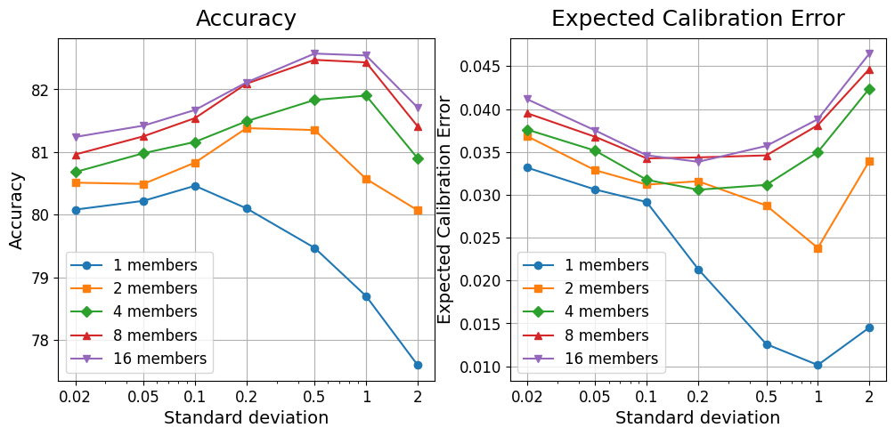
(a)

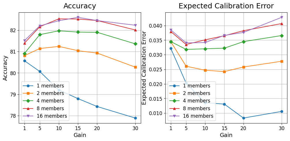
(b)

Figure 6: Accuracy and ece for different initialization methods and varying distribution parameters across different ensemble sizes for lora-Ensemble.

Appendix E Initialization of Explicit Ensemble Parameters

A pre-trained vit model is the backbone for our computer vision experiments. Correspondingly, the parameters of all members in an Explicit Ensemble are initialized to the same values across members. Initialization is a primary driver of diversity in ensemble members [Fort et al., 2019]. Hence, it is crucial to study the effect of noise in the parameter initialization on the calibration of the resulting ensemble. In the case of pre-trained model weights not having been trained on a dataset with the same number of classes, the last layer of all models is replaced completely. This means that regardless of the ensemble technique used, the weights of the last layer, which is responsible for classification, will vary across members. This variation in the weights of the classification layer is expected to contribute significantly to the diversity of the members. Nonetheless, we studied the impact of adding noise to the parameters of an Explicit Ensemble. This was done using the following formula:

$$W_{\mathrm{new}}=W+\alpha\cdot dW\,,$$ (5)

where $dW\sim\mathcal{N}(0,\sigma_{W})$. Here $\alpha$ is a scale factor to control the amount of noise and $\sigma_{W}$ is the standard deviation of the parameters within a weight matrix. This was applied to all weight matrices separately.

It is expected that the initial layers of a neural network will learn basic features, while the later layers will include dataset-specific properties. Therefore, it is assumed that adding noise to the later layers would increase diversity while maintaining pre-training. However, adding noise to the earlier layers might disrupt pre-training more significantly, especially with smaller datasets, as these parameters may not converge to meaningful values again. To address this, an experiment was set up where noise was added only to the last encoder layers of the model, increasing the number of affected encoder layers gradually. Additionally, several different noise scales $\alpha$ were tried, ranging from $1$ to $0.0001$. In the presented experiment, the last classification layer is initialized using PyTorch’s default method for linear layers. At the time of writing it is as follows:

$$W_{\mathrm{init}} =\mathrm{Unif}\left(-\sqrt{5}\cdot\sqrt{\frac{3}{fan\_in}},\sqrt{5}\cdot\sqrt{\frac{3}{fan\_in}}\right)$$ (6)

$$B_{\mathrm{init}} =\mathrm{Unif}\left(-\sqrt{\frac{1}{fan\_in}},\sqrt{\frac{1}{fan\_in}}\right).$$ (7)

Here $W$ specifies the weight matrix and $B$ is the bias. Experiments are conducted on the CIFAR-100 dataset.

E.1 Results

The most important metrics for this section are accuracy and ece. The results for adding noise to the last layer up to the last five layers are summarized in Fig. 7. Fig. 7(a) depicts the results for a single model, while Fig. 7(b) shows the results for an ensemble of 16 members.

It is evident that none of the experiments surpass the baseline of not using any additional noise beyond the random initialization of the last classification layer. After the last five layers, the results become uninteresting, as they do not vary significantly from those shown in the plots. Therefore, the presentation is truncated at five layers. Based on the presented results, no additional noise is injected into the Explicit Ensemble, and only the last layer initialization is varied.

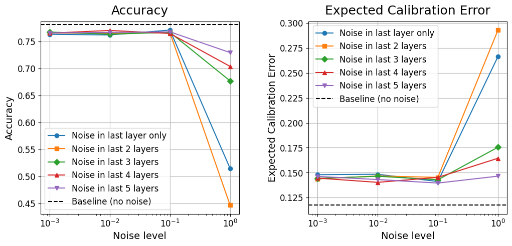
(a)

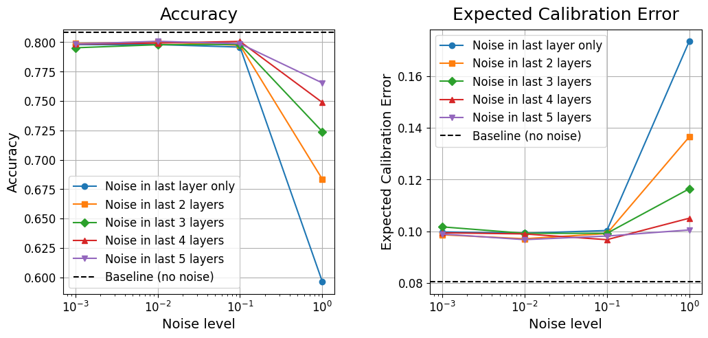
(b)

Figure 7: Accuracy and ece for different noise levels across varying numbers of layers for the Explicit Ensemble. The baseline with no noise is indicated by a dashed black line.

Appendix F AST Implementation

A different backbone is used for the experiment on the audio dataset. Specifically, we use the ast following the implementation of Gong et al. [2021], with slight modifications to fit our general architecture. Appendix G demonstrates the equivalence of our implementation. In their experiments, Gong et al. [2021] used two different types of pre-trained weights: one pre-trained on a large image dataset and the other on an audio dataset. For our research, we transfer the weights of a vision transformer model known as deit [Touvron et al., 2020], which has been pre-trained on the ImageNet dataset [Deng et al., 2009], to the original ast architecture by Gong et al. [2021]. The model has 12 layers, uses 768-dimensional patch embeddings, and the multi-head attention modules have 12 heads. This task is considered more challenging than using models pre-trained on audio datasets.

Appendix G Validation of AST Implementation

The ast model provided by Gong et al. [2021] was copied without any changes. However, the training and evaluation pipeline was adapted to fit our architecture. Correspondingly, it was essential to validate the equivalence of our implementation by training a single ast on the ESC-50 dataset. The results of our model should closely match those provided in Gong et al. [2021].

They offer two sets of pre-trained weights: one where the weights of a vit pre-trained on ImageNet [Deng et al., 2009] are transferred to ast, and another where the ast was pre-trained on AudioSet [Gemmeke et al., 2017]. To verify our implementation, we ran it using the settings provided by Gong et al. [2021] and compared the results, which are summarized in Tab. 8. The results for both pre-training modes fall within the uncertainty range provided by Gong et al. [2021]. This suggests that our pipeline yields comparable outcomes, validating our implementation for continued use.

Table 8: Comparison of the results obtained for the ast as given in Gong et al. [2021] and those obtained by our implementation. AST-S refers to the ast pre-trained on ImageNet, and AST-P refers to the AudioSet pre-training. Both results fall within the uncertainty range provided by Gong et al. [2021].

Model	Accuracy [Gong et al., 2021]	Accuracy (our implementation)
AST-S	$88.7\pm 0.7$	$88.0$
AST-P	$95.6\pm 0.4$	$95.8$

Appendix H Hyper-parameter Tuning for AST Experiment

The original training settings of the AST-S model in Gong et al. [2021] utilize a batch size of 48. However, due to the memory constraint of single GPU training on an NVIDIA Tesla A100 with 80 GB memory, replicating a batch size of 48 as in the original publication was infeasible for training an Explicit AST-S Ensemble with 8 members. Consequently, we perform minimal hyper-parameter tuning by employing a batch size of 1 for both the explicit AST-S and the lora AST-S model, exploring various learning rates. Apart from batch size and learning rate adjustments, all other settings remain consistent with Gong et al. [2021].

The hyper-parameter tuning results for the explicit model using a batch size of 1, as shown in Tab. 9, demonstrate performance similar to the original implementation with a batch size of 48, allowing for a fair comparison with our method [Gong et al., 2021]. Additionally, Tab. 10 showcases the outcomes of tuning the learning rate for our lora AST-S model.

Table 9: Single model 5-Fold cross-validation results of AST-S on ESC-50 sound dataset with different learning rates and batch size 1. The model settings selected based on accuracy for the experiments are highlighted.

Model	Learning rate	Accuracy ($\uparrow$)	ECE ($\downarrow$)
AST-S	0.00001	88.2	0.0553
AST-S	0.00005	$81.7$	$0.0933$

Table 10: Single model 5-Fold cross-validation results for our lora AST-S implementation on ESC-50 sound dataset with different learning rates and batch size 1. The model settings selected based on accuracy for the experiments are highlighted.

Model	Learning rate	Accuracy ($\uparrow$)	ECE ($\downarrow$)
LoRA AST-S	0.00001	$85.6$	$0.0447$
LoRA AST-S	0.00005	87.9	0.0487
LoRA AST-S	0.0001	$84.7$	$0.0501$
LoRA AST-S	0.0005	$24.1$	$0.0291$
LoRA AST-S	0.001	$11.8$	$0.0295$

Appendix I Computational Cost for AST Models

Similarly to the way we did for the vit models, we estimate the required resources for ast models. The resource needs are presented in Tab. 11.

Table 11: Parameter counts and computation times for an Explicit Ensemble of 8 ast models and the corresponding lora-Ensemble. Training time is the average duration for one epoch on ESC-50, with batch size 1. Inference time is the average duration of a forward pass, with batch size 1.

Method	Parameter overhead	Training time [s]	Inference time [ms]
Explicit Ensemble	$8\times 87\mathrm{M}$	$517$	$8\times 7.3$
lora-Ensemble	$1.08\times 87\mathrm{M}$	$348$	$73.9$

The number of parameters is reported for an ensemble of 8 members, with the $A$ and $B$ matrices in models using lora having a rank of 16. Training and inference times were measured on a single NVIDIA Tesla A100-80GB gpu, with a batch size of 1. Training time is given as the average wall clock time per training epoch while training on ESC-50, with 8 ensemble members. Inference time is reported as the average time for a single forward pass of an ESC-50 sample with a batch size of 1.

As mentioned in Sec. 2.1, the Explicit Ensemble processes the members sequentially, while lora-Ensemble is parallelized. However, fully parallelizing the training of ast models causes memory issues, so chunking was introduced. Thus, in lora-Ensemble models, the pass through the backbone runs in parallel, while lora modules are called sequentially. This also explains the significantly higher inference time compared to the results in Sec. 3.1. Additionally, the one-time delay incurred by PyTorch’s vmap function causes lora-Ensemble to be slightly slower at inference time.

Appendix J Hyperparameter Tuning for MC Dropout

We conducted an analysis to determine the impact of dropout probability on the accuracy and calibration of the vit with Monte Carlo dropout. Fig. 8 displays the accuracy and ece scores for various dropout probabilities. The experiment is carried out on the HAM10000 dataset with 16 members. Our findings show that a dropout probability of $0.2$ offers a good balance between accuracy and calibration.

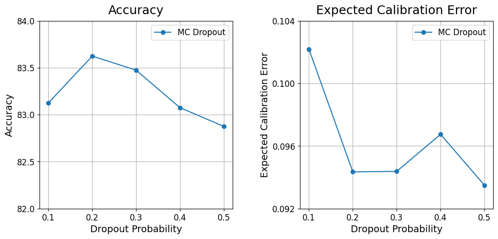
Figure 8: Accuracy and ece for different dropout probabilities methods for MC Dropout on HAM10000 dataset.

Appendix K Definitions of Evaluation Metrics

We primarily evaluate our models on accuracy and Expected Calibration Error [ECE, Guo et al., 2017]. In the following section, we present the formulations used in our implementations.

K.1 Accuracy

The accuracy is implemented instance-wise as follows:

$$\mathrm{Acc}=\frac{1}{N}\sum_{i=1}^{N}\frac{\lvert\hat{y}_{i}\cap y_{i}\rvert}{\lvert\hat{y}_{i}\cup y_{i}\rvert}$$ (8)

Here $y_{i}$ denotes the true label of the sample $i$, $\hat{y}_{i}$ is the predicted label of the sample $i$, and $N$ means the total number of samples.

K.2 Expected Calibration Error

The ece is a widely used metric for measuring the calibration of neural networks. We use the definition given in Guo et al. [2017]. ece is defined as the expected difference between accuracy and confidence across several bins. We first need to define accuracy and confidence per bin $B_{m}$ as follows:

$$\mathrm{Acc}(B_{m}) =\frac{1}{\lvert B_{m}\rvert}\sum_{i\in B_{m}}\mathbf{1}(\hat{y}_{i}=y_{i}),$$ (9)

$$\mathrm{Conf}(B_{m}) =\frac{1}{\lvert B_{m}\rvert}\sum_{i\in B_{m}}\hat{p}_{i}.$$ (10)

Again, $y_{i}$ and $\hat{y}_{i}$ denote the true and predicted labels of sample $i$ respectively, and $\hat{p}_{i}$ is the predicted confidence of sample $i$. With this the ece is given as:

$$\mathrm{ECE}=\sum_{m=1}^{M}\frac{\lvert B_{m}\rvert}{n}\lvert\mathrm{Acc}(B_{m})-\mathrm{Conf}(B_{m})\rvert$$ (11)

K.3 Supplementary Evaluation Metrics

In addition to accuracy and ece, we have calculated several other scores that have been used in the context of probabilistic deep learning. These scores are defined as follows.

Macro F1-score is defined as

$$F1=\frac{1}{C}\sum_{j=1}^{C}\frac{2p_{j}r_{j}}{p_{j}+r_{j}},$$ (12)

where $r_{j}$ represents the Recall of class $j$, defined as $r_{j}=\frac{TP}{TP+FN}$, and $p_{j}$ represents the Precision of class $j$, defined as $p_{j}=\frac{TP}{TP+FP}$, and $C$ refers to the number of classes, Here, $TP$, $FP$, and $FN$ denote True Positives, False Positives, and False Negatives respectively.

Negative Log-Likelihood (NLL) is defined as

$$NLL=-\frac{1}{N}\sum_{i=1}^{N}\sum_{j=1}^{C}\left(y_{i,j}\log\hat{p}_{i,j}\right)=-\frac{1}{N}\sum_{i=1}^{N}\log\hat{p}_{i},$$ (13)

where $N$ denotes the number of datapoints, $C$ the number of classes, $y_{i,j}$ is 1 if the true label of point $i$ is $j$ and 0 otherwise and $\hat{p}_{i,j}$ is the predicted probability of sample $i$ belonging to class $j$.

For Brier score we take the definition by Brier [1950], which is as follows:

$$BS=\frac{1}{N}\sum_{i=1}^{N}\sum_{j=1}^{C}(\hat{p}_{i,j}-y_{i,j})^{2},$$ (14)

where $N$ denotes the number of datapoints, $C$ the number of classes, $y_{i,j}$ is 1 if the true label of point $i$ is $j$ and zero otherwise and $\hat{p}_{i,j}$ is the predicted probability of sample $i$ belonging to class $j$.

References

- Aghajanyan et al. [2020] A. Aghajanyan, S. Gupta, and L. Zettlemoyer. Intrinsic Dimensionality Explains the Effectiveness of Language Model Fine-Tuning. In 59th Annual Meeting of the Association for Computational Linguistics and the 11th International Joint Conference on Natural Language Processing, 2020.
- Blundell et al. [2015] C. Blundell, J. Cornebise, K. Kavukcuoglu, and D. Wierstra. Weight Uncertainty in Neural Networks. In 32nd International Conference on Machine Learning, 2015.
- Brier [1950] G. W. Brier. Verification Of Forecasts Expressed In Terms Of Probability. Monthly Weather Review, 78, 1950.
- Brown et al. [2020] T. B. Brown, B. Mann, N. Ryder, M. Subbiah, J. Kaplan, P. Dhariwal, A. Neelakantan, P. Shyam, G. Sastry, A. Askell, S. Agarwal, A. Herbert-Voss, G. Krueger, T. Henighan, R. Child, A. Ramesh, D. M. Ziegler, J. Wu, C. Winter, C. Hesse, M. Chen, E. Sigler, M. Litwin, S. Gray, B. Chess, J. Clark, C. Berner, S. McCandlish, A. Radford, I. Sutskever, and D. Amodei. Language Models are Few-Shot Learners. In Advances in Neural Information Processing Systems, 2020.
- Chen et al. [2014] T. Chen, E. B. Fox, and C. Guestrin. Stochastic Gradient Hamiltonian Monte Carlo. In 31st International Conference on Machine Learning, 2014.
- Conrad [2023] B. Conrad. Fine-tuning Vision Transformers, 2023. URL https://github.com/bwconrad/vit-finetune. Accessed: 2024-05-20.
- Cui et al. [2019] Y. Cui, M. Jia, T. Y. Lin, Y. Song, and S. Belongie. Class-balanced loss based on effective number of samples. In IEEE Computer Society Conference on Computer Vision and Pattern Recognition, 2019.
- Deng et al. [2009] J. Deng, W. Dong, R. Socher, L.-J. Li, Kai Li, and Li Fei-Fei. ImageNet: A large-scale hierarchical image database. In IEEE Conference on Computer Vision and Pattern Recognition, 2009.
- Der Kiureghian and Ditlevsen [2009] A. Der Kiureghian and O. Ditlevsen. Aleatory or epistemic? Does it matter? Structural Safety, 31(2), 2009.
- Dosovitskiy et al. [2020] A. Dosovitskiy, L. Beyer, A. Kolesnikov, D. Weissenborn, X. Zhai, T. Unterthiner, M. Dehghani, M. Minderer, G. Heigold, S. Gelly, J. Uszkoreit, and N. Houlsby. An Image is Worth 16x16 Words: Transformers for Image Recognition at Scale. In 9th International Conference on Learning Representations, 2020.
- Durasov et al. [2020] N. Durasov, T. Bagautdinov, P. Baque, and P. Fua. Masksembles for Uncertainty Estimation. In IEEE Computer Society Conference on Computer Vision and Pattern Recognition, 2020.
- Fort et al. [2019] S. Fort, H. Hu, and B. Lakshminarayanan. Deep Ensembles: A Loss Landscape Perspective, 2019. arXiv: 1912.02757.
- Gal and Ghahramani [2015] Y. Gal and Z. Ghahramani. Dropout as a Bayesian Approximation: Representing Model Uncertainty in Deep Learning. In 33rd International Conference on Machine Learning, 2015.
- Gemmeke et al. [2017] J. F. Gemmeke, D. P. Ellis, D. Freedman, A. Jansen, W. Lawrence, R. C. Moore, M. Plakal, and M. Ritter. Audio Set: An ontology and human-labeled dataset for audio events. In IEEE International Conference on Acoustics, Speech and Signal Processing, 2017.
- Glorot and Bengio [2010] X. Glorot and Y. Bengio. Understanding the difficulty of training deep feedforward neural networks. In 13th International Conference on Artificial Intelligence and Statistics, 2010.
- Golnari [2023] P. A. Golnari. LoRA-Enhanced Distillation on Guided Diffusion Models, 2023. arXiv: 2312.06899.
- Gong et al. [2021] Y. Gong, Y. A. Chung, and J. Glass. AST: Audio Spectrogram Transformer. In Annual Conference of the International Speech Communication Association, 2021.
- Graves [2011] A. Graves. Practical Variational Inference for Neural Networks. In Advances in Neural Information Processing Systems, 2011.
- Guo et al. [2017] C. Guo, G. Pleiss, Y. Sun, and K. Q. Weinberger. On Calibration of Modern Neural Networks. In 34th International Conference on Machine Learning, 2017.
- Gustafsson et al. [2019] F. K. Gustafsson, M. Danelljan, and T. B. Schon. Evaluating Scalable Bayesian Deep Learning Methods for Robust Computer Vision. In IEEE Computer Society Conference on Computer Vision and Pattern Recognition Workshops, 2019.
- Havasi et al. [2020] M. Havasi, R. Jenatton, S. Fort, J. Z. Liu, J. Snoek, B. Lakshminarayanan, A. M. Dai, and D. Tran. Training independent subnetworks for robust prediction. In 9th International Conference on Learning Representations, 2020.
- Hu et al. [2021] E. Hu, Y. Shen, P. Wallis, Z. Allen-Zhu, Y. Li, S. Wang, L. Wang, and W. Chen. LoRA: Low-Rank Adaptation of Large Language Models. In 10th International Conference on Learning Representations, 2021.
- Huang et al. [2017] G. Huang, Y. Li, G. Pleiss, Z. Liu, J. E. Hopcroft, and K. Q. Weinberger. Snapshot Ensembles: Train 1, Get M for Free. In International Conference on Learning Representations, 2017.
- Izmailov et al. [2021] P. Izmailov, S. Vikram, M. D. Hoffman, and A. G. Wilson. What Are Bayesian Neural Network Posteriors Really Like? In Proceedings of Machine Learning Research, 2021.
- Jiang et al. [2024] A. Q. Jiang, A. Sablayrolles, A. Roux, A. Mensch, B. Savary, C. Bamford, D. S. Chaplot, D. d. l. Casas, E. B. Hanna, F. Bressand, G. Lengyel, G. Bour, G. Lample, L. R. Lavaud, L. Saulnier, M.-A. Lachaux, P. Stock, S. Subramanian, S. Yang, S. Antoniak, T. L. Scao, T. Gervet, T. Lavril, T. Wang, T. Lacroix, and W. E. Sayed. Mixtral of Experts, 2024. arXiv: 2401.04088.
- Krizhevsky [2009] A. Krizhevsky. Learning Multiple Layers of Features from Tiny Images. University of Toronto, 2009.