Boosting Robustness by Clipping Gradients in Distributed Learning

Abstract

Robust distributed learning consists in achieving good learning performance despite the presence of misbehaving workers. State-of-the-art (SOTA) robust distributed gradient descent (Robust-DGD) methods, relying on robust aggregation, have been proven to be optimal: Their learning error matches the lower bound established under the standard heterogeneity model of $(G,B)$-gradient dissimilarity. The learning guarantee of SOTA Robust-DGD cannot be further improved when model initialization is done arbitrarily. However, we show that it is possible to circumvent the lower bound, and improve the learning performance, when the workers’ gradients at model initialization are assumed to be bounded. We prove this by proposing pre-aggregation clipping of workers’ gradients, using a novel scheme called adaptive robust clipping (ARC). Incorporating ARC in Robust-DGD provably improves the learning, under the aforementioned assumption on model initialization. The factor of improvement is prominent when the tolerable fraction of misbehaving workers approaches the breakdown point. ARC induces this improvement by constricting the search space, while preserving the robustness property of the original aggregation scheme at the same time. We validate this theoretical finding through exhaustive experiments on benchmark image classification tasks.

1 Introduction

Distributed machine learning, a.k.a. federated learning, has emerged as a dominant paradigm to cope with the increasing computational cost of learning tasks, mainly due to growing model sizes and datasets [25]. Worker machines, holding each a fraction of the training dataset, collaborate over a network to learn an optimal common model over the collection of their datasets. Workers typically collaborate with the help of a central coordinator, that we call server [36]. Besides scalability, distributed learning is also helpful in preserving data privacy, since the workers do not have to share their local datasets during the learning.

Conventional distributed learning algorithms are known to be vulnerable to misbehaving workers that could behave unpredictably [7, 25, 18]. Misbehavior may result from software and hardware bugs, data poisoning, or malicious players controlling part of the network. In the parlance of distributed computing, misbehaving workers are referred to as Byzantine [32]. Due to the growing influence of distributed learning in critical public-domain applications, such as healthcare [38] and finance [34], the problem of robustness to misbehaving workers, a.k.a. robust distributed learning, has received significant attention in the past [7, 44, 12, 14, 27, 17, 3, 13].

Robust distributed learning algorithms primarily rely on robust aggregation, such as coordinate-wise trimmed mean (CWTM) [44], geometric median (GM) [10] and multi-Krum (MK) [7]. Specifically, in a robust distributed gradient descent (Robust-DGD) method, the server aggregates the workers’ local gradients using a robust aggregation rule, instead of simply averaging them. This protects the learning procedure from erroneous gradients sent by misbehaving workers. Recent work has made significant improvements over these aggregation rules: by incorporating a pre-aggregation step such as bucketing [27, 17] and nearest-neighbor mixing (NNM) [3] to tackle gradient dissimilarity that results from data heterogeneity. The learning guarantee of a resulting Robust-DGD method has been proven to be optimal [4], i.e., it cannot be improved unless additional assumptions are made, under the standard heterogeneity model of $(G,B)$-gradient dissimilarity [28].

Despite the theoretical tightness of state-of-the-art (SOTA) Robust-DGD, we demonstrate that its performance can be improved in pragmatic cases wherein model initialization incurs bounded errors on workers’ local data. We do so by proposing clipping of workers’ gradients prior to their aggregation (at the server) using a novel clipping scheme, named adaptive robust clipping (ARC). We show that incorporating ARC provably improves the robustness of Robust-DGD when the local gradients at the initial model estimate are bounded. The factor of improvement is prominent when the tolerable fraction of misbehaving workers approaches the breakdown point, established in [4] under $(G,B)$-gradient dissimilarity. In general, when the local gradients can be arbitrarily large at initialization, ARC recovers the original learning guarantee of Robust-DGD.

Main results & contributions.

We consider a system comprising $n$ workers and a server. The goal is to tolerate up to $f$ misbehaving (a.k.a. adversarial) workers. The impact of data heterogeneity is characterized by the standard definition of $(G,B)$-gradient dissimilarity [28], recalled in Section 2.

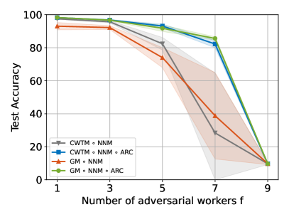
Figure 1: Worst-case maximal accuracies across several types of misbehaviour (see Section 6) of CWTM $\circ$ NNM and GM $\circ$ NNM, with ARC and without (i.e., no clipping), for a heterogeneously distributed MNIST dataset with $10$ honest workers. Heterogeneity is simulated using Dirichlet [23] distribution of parameter $\alpha=0.5$.

(1) Adaptive robust clipping (ARC). We propose ARC, wherein prior to aggregating the gradients, the server clips the largest $k\coloneqq\left\lfloor{2(f/n)(n-f)}\right\rfloor$ gradients using a clipping parameter given by the (Euclidean) norm of the $(k+1)$-th largest gradient. We prove 2 crucial properties: ARC (i) preserves the robustness guarantee of original aggregation and (ii) constrains an adversarial gradient’s norm by that of an honest (non-adversarial) worker’s gradient.

(2) Improved learning error. Under $(G,B)$-gradient dissimilarity, [4] proves a lower bound on the learning error in the presence of adversarial workers. We show, however, that this lower bound can be circumvented under the assumption that the honest workers’ gradients are bounded at model initialization. Specifically, under this assumption, we prove that incorporating ARC in Robust-DGD improves the learning error beyond the lower bound when $f/n$ approaches the breakdown point. Thanks to its two aforementioned properties, ARC induces this improvement by effectively reducing the heterogeneity from $(G,B)$ to $(G+B\rho,0)$-gradient dissimilarity, where $\rho$ depends linearly on the norm of workers’ gradients at model initialization. We remark that the above assumption on model initialization is often satisfiable in practice [15].

(3) Empirical validation. We conduct experiments on MNIST [11], Fashion-MNIST [42], and CIFAR-10 [31], under several data heterogeneity and adversarial regimes. Our results show that ARC boosts the performance of SOTA robust aggregation methods, especially when considering a large number of adversarial workers. A preview of our results on MNIST is shown in Figure 1. We make similar observations on the effectiveness of ARC in scenarios of high heterogeneity (see Figure 3).

Related work.

Gradient clipping is a well-known technique for tackling exploding gradients in deep learning [16]. It has been extensively analyzed in the centralized setting [46, 45, 30], with applications to differential privacy [39]. There is also some work analyzing the impact of clipping in non-robust distributed learning [47, 29]. It has been shown that the clipping of local gradients causes distributed gradient descent to diverge. This motivates the need for an analysis of the clipping technique in our adversarial setting, and also hints at the inadequacy of clipping with a fixed threshold.

In the context of robust distributed learning, prior work has proposed iterative clipping for robust aggregation [26]. The analysis, however, cannot be applied to study the impact of pre-aggregation clipping that we consider. An adaptive gradient clipping scheme was also proposed for robust aggregation in [20, 33]. However, the robustness guarantees are only provided for strongly convex loss functions and under a specific redundancy condition that is inadequate for our non-convex machine learning setting. Other work [37, 14, 3] has only used static pre-aggregation clipping to enhance the empirical robustness of the proposed algorithms, but fail to provide any theoretical guarantees. Recent work [35] has proposed clipping of the gradient differences, in conjunction with variance reduction, to tackle partial worker participation when adversarial workers can form a majority. Our focus is however different, as we consider the impact of pre-aggregation clipping on the robustness obtained by a general class of aggregation rules.

Lastly, prior work [19, 48, 5] has also considered the challenge of privacy preservation alongside robustness in distributed learning. In this line of work, the gradients are assumed to have bounded norms in order to control the sensitivity of the algorithm, as is common in differential privacy (DP) [1]. This is often ensured in practice by clipping the gradients using a static clipping parameter. Our findings suggest that it is better to use adaptive clipping instead of static clipping. Nevertheless, thoroughly analysing ARC in the context of DP remains an interesting research direction.

Paper outline.

Section 2 presents the problem statement. Section 3 presents the background on robust distributed learning, while Section 4 introduces ARC and its useful properties. Section 5 presents the convergence analysis of Robust-DGD with ARC, and characterizes the improvement in its robustness. Section 6 presents our empirical results. Lastly, Section 7 presents concluding remarks. Appendix A presents the computational complexity of ARC. Appendices B and C contain proofs for results presented in Sections 4 and 5, respectively. Appendix D describes the experimental setup, while Appendices E and F include additional experimental results.

2 Problem Statement

We consider the problem of distributed learning in the server-based architecture. The system comprises $n$ workers represented by $w_{1},\dots,w_{n}$, that collaborate with the help of a trusted server. The workers hold local datasets $\mathcal{D}_{1},\dots,\mathcal{D}_{n}$ respectively, each composed of $m$ data points from an input space $\mathcal{Z}$. Specifically, for any $i\in[n]$, $\mathcal{D}_{i}\coloneqq\{z_{1}^{(i)},\dots,z_{m}^{(i)}\}\subset\mathcal{Z}^{m}$. For a given model parameterized by vector $\theta\in\mathbb{R}^{d}$, $d$ being the number of trainable parameters in the model, each worker $w_{i}$ incurs a loss given by the loss function $\mathcal{L}_{i}{(\theta)}\coloneqq\frac{1}{m}\sum_{k=1}^{m}\ell(\theta,z_{k}^{(i)})\enspace$, where $\ell:\mathbb{R}^{d}\times\mathcal{Z}\rightarrow\mathbb{R}$ is the point-wise loss. We make the following standard assumptions [8]: (i) the point-wise loss function $\ell$ is differentiable with respect to $\theta$. (ii) For all $i\in[n]$, $\mathcal{L}_{i}$ is $L$-Lipschitz smooth, i.e., there exists $L\in\mathbb{R}^{+}$ such that all $\theta,\theta^{\prime}\in\mathbb{R}^{d}$, $\left\lVert{\nabla\mathcal{L}_{i}(\theta{})-\nabla\mathcal{L}_{i}(\theta{}^{\prime})}\right\rVert\leq L\left\lVert{\theta{}-\theta{}^{\prime}}\right\rVert$. In the ideal setting where all workers are assumed to be honest, i.e., follow the prescribed algorithm correctly, the server aims to minimize the global average loss function given by $\mathcal{L}(\theta{})\coloneqq\frac{1}{n}\sum_{i=1}^{n}\mathcal{L}_{i}(\theta{})$. However, this learning objective is rendered vacuous when some workers could be adversarial, described in the following.

Robust distributed learning. A robust distributed learning algorithm aims to output a good model despite the presence of some adversarial (a.k.a., Byzantine [32]) workers in the system [40, 44, 3]. Specifically, the goal is to design a distributed learning algorithm that can tolerate up to $f$ adversarial workers, of a priori unknown identity, out of $n$ workers. Adversarial workers need not follow a prescribed algorithm, and can send arbitrary information to the server. In the context of distributed gradient descent, adversarial workers can send incorrect gradients to the server [6, 2, 43, 27]. We let $\mathcal{H}\subseteq[n]$, with $\left\lvert{\mathcal{H}}\right\rvert=n-f$, denote the set of honest workers that do not deviate from an algorithm. The objective of the server is to minimize the honest workers’ average loss function given by

$$\mathcal{L}_{\mathcal{H}}(\theta)\coloneqq\frac{1}{\left\lvert{\mathcal{H}}\right\rvert}\sum_{i\in\mathcal{H}}\mathcal{L}_{i}(\theta),~{}\forall\theta\in\mathbb{R}^{d}.$$

While we can find a minimum of $\mathcal{L}_{\mathcal{H}}(\theta)$ when $\mathcal{L}_{\mathcal{H}}$ is convex, in general however the loss function is non-convex, and the optimization problem is NP-hard [9]. Therefore, we aim to find a stationary point of $\mathcal{L}_{\mathcal{H}}$ instead, i.e., $\theta^{*}$ such that $\left\lVert{\nabla\mathcal{L}_{\mathcal{H}}(\theta^{\ast})}\right\rVert=0$. Formally, we define robustness to adversarial workers by $(f,\epsilon)$-resilience [3].

Definition 2.1.

A distributed learning algorithm $\mathcal{A}$ is said to be $(f,\varepsilon)$-resilient if, despite the presence of $f$ adversarial workers, $\mathcal{A}$ enables the server to output a model $\hat{\theta}$ such that $\mathop{{}\mathbb{E}}\left[{\left\lVert{\nabla\mathcal{L}_{\mathcal{H}}\left(\hat{\theta}\right)}\right\rVert^{2}}\right]\leq\varepsilon$, where the expectation $\mathop{{}\mathbb{E}}\left[{\cdot}\right]$ is over the randomness of the algorithm.

If a distributed learning algorithm $\mathcal{A}$ is $(f,\varepsilon)$-resilient then it can tolerate up to $f$ adversarial workers. Thus, $f/n$ is referred to as the maximum tolerable fraction of adversarial workers for $\mathcal{A}$. It is standard in robust distributed learning to design an algorithm using $f$ as a parameter [40, 7, 44, 27, 17, 3].

Data heterogeneity. In the context of distributed learning, data heterogeneity is characterized by the following standard notion of $(G,B)$-gradient dissimilarity [41, 28, 27, 17, 4].

Definition 2.2.

Loss functions $\mathcal{L}_{i},\;i\in\mathcal{H},$ are said to satisfy $(G,B)$-gradient dissimilarity if,

$$\frac{1}{\left\lvert{\mathcal{H}}\right\rvert}\sum_{i\in\mathcal{H}}\left\lVert{\nabla\mathcal{L}_{i}(\theta)-\nabla\mathcal{L}_{\mathcal{H}}(\theta)}\right\rVert^{2}\leq G^{2}+B^{2}\left\lVert{\nabla\mathcal{L}_{\mathcal{H}}(\theta)}\right\rVert^{2},\quad\forall\theta\in\mathbb{R}^{d}.$$

3 Relevant Background

We present in this section useful precursors on robust distributed learning.

General limitations on robustness. Note that $(f,\varepsilon)$-resilience is impossible (for any $\varepsilon$) when $f/n\geq 1/2$ [20]. Moreover, even for $f/n<1/2$, it is generally impossible to achieve $(f,\varepsilon)$-resilience for arbitrarily small $\varepsilon$ due to the disparity amongst the local datasets $\mathcal{D}_{i},\;i\in\mathcal{H}$ (a.k.a., data heterogeneity) [33]. Henceforth, we assume that $n>2f$ by default. Under $(G,B)$-gradient dissimilarity, we have the following lower bound on the achievable resilience.

Lemma 3.1 (Non-convex extension of Theorem 1 in [4]).

Under $(G,B)$-gradient dissimilarity, a distributed learning algorithm $\mathcal{A}$ satisfies $(f,\varepsilon)$-resilience only if $\frac{f}{n}<\frac{1}{2+B^{2}}$ and $\varepsilon\geq\frac{1}{4}\cdot\frac{f}{n-(2+B^{2})f}G^{2}$.

For a given distributed learning problem, the minimum fraction of adversarial workers that renders any distributed learning algorithm ineffective is referred the breakdown point [18, 4]. Thus, according to Lemma 3.1, there exists a distributed learning problem satisfying $(G,B)$-gradient dissimilarity whose breakdown point is given by $1/(2+B^{2})$.

In the ideal setting, i.e., when all the workers are honest, the server can execute the classic distributed gradient descent (DGD) method in collaboration with the workers to find a stationary point of the global average loss function. In DGD, the server maintains the model, which is updated periodically using the average of the gradients computed by the workers on their local datasets. The averaging of the gradients is rendered ineffective when some workers are adversarial, i.e., they can send malicious vectors posing as their gradients to the server [18]. To remedy this, averaging is replaced with robust aggregation, e.g., coordinate-wise trimmed mean (CWTM) and median (CWMed) [44], geometric median (GM) [10], and multi-Krum (MK) [7]. Useful properties of a resulting Robust-DGD method, which is summarized in Algorithm 1, are recalled below.

Robust distributed gradient descent (Robust-DGD). In Robust-DGD, robust aggregation protects the learning procedure from incorrect gradients sent by the adversarial workers. The robustness of an aggregation can be quantified by the following property of $(f,\kappa)$-robustness, proposed in [3].

Algorithm 1 Robust Distributed Gradient Descent (Robust-DGD)

  Initialization: Server chooses a model ${{\theta}_{1}}\in\mathbb{R}^{d}$, a learning rate $\gamma\in\mathbb{R}^{+}$ and a robust aggregation rule $\mathbf{F}:\mathbb{R}^{n\times d}\to\mathbb{R}^{d}$.

  for $t=1$ to $T$ do

     Server broadcasts ${{\theta}_{t}}$ to all workers.

     for each honest worker ${{w}_{i}}$ in parallel do

        Compute local gradient ${{g}^{\left({i}\right)}_{t}}\coloneqq\nabla{\mathcal{L}_{i}({{\theta}_{t}})}$, and send ${{g}^{\left({i}\right)}_{t}}$ to Server.

        // An adversarial worker ${{w}_{j}}$ can send an arbitrary vector in $\mathbb{R}^{d}$ for ${{g}^{\left({j}\right)}_{t}}$

     end for

     Server computes $R_{t}\coloneqq\mathbf{F}\left({{g}^{\left({1}\right)}_{t}},\dots,\,{{g}^{\left({n}\right)}_{t}}\right)$.

     Server computes the updated model ${{\theta}_{t+1}}\coloneqq{{\theta}_{t}}-\gamma\,R_{t}$ .

  end for

  Output: Server outputs $\hat{{{\theta}}}$ chosen uniformly at random from $\{{{\theta}_{1}},\ldots,\,{{\theta}_{T}}\}$.

Definition 3.2.

Aggregation rule ${\mathbf{F}:\mathbb{R}^{n\times d}\to\mathbb{R}^{d}}$ is said to be $(f,\kappa)$-robust if there exists $\kappa\in\mathbb{R}$ such that, for all $x_{1},\ldots,x_{n}\in\mathbb{R}^{d}$ and any set $S\subseteq[n]$, $\left\lvert{S}\right\rvert=n-f$, the following holds true:

$$\left\lVert{\mathbf{F}(x_{1},\ldots,x_{n})-\overline{x}_{S}}\right\rVert^{2}\leq\frac{\kappa}{\left\lvert{S}\right\rvert}\sum_{i\in S}\left\lVert{x_{i}-\overline{x}_{S}}\right\rVert^{2}\enspace,\quad\text{where }~{}\overline{x}_{S}=\frac{1}{\left\lvert{S}\right\rvert}\sum\limits_{i\in S}x_{i}.$$

We refer to $\kappa$ as the robustness coefficient.

The property of $(f,\kappa)$-robustness encompasses several robust aggregations, including the ones mentioned above and more (e.g., see [3]). It has been shown that an aggregation rule is $(f,\kappa)$-robust only if $\kappa\geq\frac{f}{n-2f}$ [3]. Importantly, the asymptotic error of Robust-DGD with $(f,\kappa)$-robust aggregation, where $\kappa\in\mathcal{O}(f/(n-2f))$, matches the lower bound (recalled in Lemma 3.1) [4]. Note that all the aforementioned aggregation rules, i.e., CWTM, CWMed, GM and MK, attain optimal robustness, i.e., are $(f,\mathcal{O}\left(f/(n-2f)\right))$-robust, when composed with the pre-aggregation step: nearest neighbor mixing (NNM) [3]. Specifically, we recall the following result.

Lemma 3.3 (Lemma 1 in [3]).

For $\mathbf{F}\in\left\{\mathbf{CWTM},\mathbf{CWMed},\mathbf{GM},\mathbf{MK}\right\}$, the composition $\mathbf{F}\circ\mathbf{NNM}$ is $(f,\kappa)$-robust with

$$\kappa\leq\frac{8f}{n-f}\left(1+\left(1+\frac{f}{n-2f}\right)^{2}\right).$$

Thus, if $n\geq(2+\delta)f$ for $\delta>0$, then $\mathbf{F}\circ\mathbf{NNM}$ is $(f,\kappa)$-robust with $\kappa\leq\frac{16f}{n-f}\left(\frac{\delta+1}{\delta}\right)^{2}\in\mathcal{O}\left(\frac{f}{n-2f}\right)$.

Convergence of Robust-DGD. Lastly, we recall the convergence result for Robust-DGD with an $(f,\kappa)$-robust aggregation $\mathbf{F}$. We let $\mathcal{L}_{\mathcal{H}}^{*}$ denote the minimum value of $\mathcal{L}_{\mathcal{H}}({{\theta}})$.

Lemma 3.4 (Theorem 2 in [4]).

Consider Algorithm 1 with $\gamma\leq 1/L$. Let $\Delta_{o}\in\mathbb{R}^{+}$ such that $\mathcal{L}_{\mathcal{H}}({{\theta}_{1}})-\mathcal{L}_{\mathcal{H}}^{*}\leq\Delta_{o}$. If the aggregation rule $\mathbf{F}$ is $(f,\kappa)$-robust with $\kappa B^{2}<1$, then

$$\frac{1}{T}\sum_{t=1}^{T}\left\lVert{\nabla\mathcal{L}_{\mathcal{H}}({{\theta}_{t}})}\right\rVert^{2}\leq\frac{2\Delta_{o}}{(1-\kappa B^{2})\gamma T}+\frac{\kappa G^{2}}{1-\kappa B^{2}}.$$

Thus, when $\kappa\in\mathcal{O}\left(f/(n-2f)\right)$ (and smaller than $1/B^{2}$), Robust-DGD is optimal, i.e., its error matches the lower bound recalled in Lemma 3.1, as soon as $T\geq\Delta_{o}/\gamma\kappa G^{2}$.

4 Adaptive Robust Clipping (ARC) and its Properties

In this section, upon presenting a preliminary observation on the fragility of static clipping, we introduce adaptive robust clipping (i.e., ARC). Lastly, we present some useful properties of ARC.

For a clipping parameter $C\in\mathbb{R}^{+}$ and a vector $x\in\mathbb{R}^{d}$, we denote $\mathrm{clip}_{C}(x)\coloneqq\min\left(1,\frac{C}{\left\lVert{x}\right\rVert}\right)x$. For a set of $n$ vectors $x_{1},\dots,x_{n}\in\mathbb{R}^{d}$, we denote $\mathbf{Clip}_{C}(x_{1},\dots,x_{n})\coloneqq(\mathrm{clip}_{C}(x_{1}),\dots,\mathrm{clip}_{C}(x_{n}))\enspace.$

Let $\mathbf{F}$ be an $(f,\kappa)$-robust aggregation. Given a set of $n$ vectors $x_{1},\ldots,x_{n}$, let $\mathbf{F}\circ\mathbf{Clip}_{C}(x_{1},\dots,x_{n})\coloneqq\mathbf{F}\left(\mathbf{Clip}_{C}(x_{1},\dots,x_{n})\right)$. We make the following observation.

Lemma 4.1.

For any fixed $C\in\mathbb{R}^{+}$ and $\kappa^{\prime}\geq 0$, ${\mathbf{F}\circ\mathbf{Clip}_{C}}$ is not $(f,\kappa^{\prime})$-robust.

This means that if the clipping threshold is a priori fixed, i.e., independent from the input vectors, pre-aggregation clipping does not preserve the robustness of the original aggregation. This fragility of such static clipping is also apparent in practice, as shown by our experimental study in Appendix F.

Description of ARC. In ARC, the clipping threshold is determined according to the input vectors. More precisely, ARC clips the largest $k=\left\lfloor{2(f/n)(n-f)}\right\rfloor$ vectors using a clipping parameter given by the norm of the $(k+1)$-th largest input vector. The overall scheme is formally presented in Algorithm 2, and its computational complexity is $\mathcal{O}(nd+n\log(n))$ (see Appendix A). ARC is adaptive in the sense that the clipping threshold $C$ is not fixed but depends on the input vectors.

Algorithm 2 Adaptive Robust Clipping (ARC)

  Input: $f$ and $x_{1},\ldots,x_{n}\in\mathbb{R}^{d}$.

  Find a permutation $\pi:[n]\to[n]$ such that $\left\lVert{x_{\pi(1)}}\right\rVert\geq\left\lVert{x_{\pi(2)}}\right\rVert\ldots\geq\left\lVert{x_{\pi(n)}}\right\rVert$.

  Set $k=\left\lfloor{2\frac{f}{n}(n-f)}\right\rfloor$ and $C=\left\lVert{x_{\pi(k+1)}}\right\rVert$.

  Output: $\mathbf{Clip}_{C}(x_{1},\ldots,x_{n})$ .

Properties of ARC. We present below important properties of ARC. Let $\mathbf{F}$ be an $(f,\kappa)$-robust aggregation rule and $\mathbf{F}\circ\mathbf{ARC}(x_{1},\dots,x_{n})\coloneqq\mathbf{F}(\mathbf{ARC}(x_{1},\dots,x_{n}))$ .

Theorem 4.2.

If $\mathbf{F}$ is $(f,\kappa)$-robust, then $\mathbf{F}\circ\mathbf{ARC}$ is $\left(f,\kappa+\frac{2f}{n-2f}\right)$-robust.

Since $\kappa\geq\frac{f}{n-2f}$ (recalled in Section 3), Theorem 4.2 implies that $\mathbf{F}\circ\mathbf{ARC}$ is $\left(f,3\kappa\right)$-robust. In other words, ARC preserves the robustness of the original aggregation scheme.

Besides preserving robustness in the context of Robust-DGD, ARC also limits the norms of adversarial workers’ gradients by the norm of an honest worker’s gradient. Specifically, when $f/n<1/2$, the clipping threshold $C$ in ARC is bounded by $\max_{i\in\mathcal{H}}\left\lVert{x_{i}}\right\rVert$ (see Appendix C.2). This property is useful in proving our convergence result, stated below in Theorem 5.1. Proofs for Lemma 4.1 and Theorem 4.2 are deferred to Appendix B.

5 Learning Guarantee of Robust-DGD with ARC

In this section, we first present our convergence result for Robust-DGD with ARC (or Robust-DGD $\circ$ ARC), and then characterize its improvement over the lower bound recalled in Lemma 3.1. Specifically, throughout this section, we consider Algorithm 1 with aggregation $\mathbf{F}\circ\mathbf{ARC}$, i.e., in each learning step $t$, $R_{t}\coloneqq\mathbf{F}\circ\mathbf{ARC}\left({{g}^{\left({1}\right)}_{t}},\dots,\,{{g}^{\left({n}\right)}_{t}}\right)$ . Note that, since we have already shown in Theorem 4.2 that $\mathbf{F}\circ\mathbf{ARC}$ is $(f,3\kappa)$-robust, a general convergence result for Robust-DGD $\circ$ ARC follows verbatim from Lemma 3.4, replacing $\kappa$ with $3\kappa$. However, we obtain below an alternative convergence result that enables us to show the improvement in learning error due to ARC.

5.1 Convergence of Robust-DGD with ARC

We assume that, for any set of vectors $x_{1},\ldots,x_{n}\in\mathbb{R}^{d}$, $\left\lVert{\mathbf{F}\left(x_{1},\ldots,x_{n}\right)}\right\rVert\leq\max_{i\in[n]}\left\lVert{x_{i}}\right\rVert$. This assumption can be made without loss of generality, the reason for which is deferred to Appendix C.1.

Theorem 5.1.

Let $\mathbf{F}$ be $(f,\kappa)$-robust. Let $\Delta_{o}$ and $\rho$ be real values such that $\mathcal{L}_{\mathcal{H}}({{\theta}_{1}})-\mathcal{L}_{\mathcal{H}}^{*}\leq\Delta_{o}$ and $\max_{i\in\mathcal{H}}\left\lVert{\nabla\mathcal{L}_{i}({{\theta}_{1}})}\right\rVert\leq\exp\left(-\frac{\Delta_{o}}{\kappa G^{2}}L\right)\rho$. If $\gamma=\min\left\{\left(\frac{\Delta_{o}}{\kappa G^{2}}\right)\frac{1}{T},~{}\frac{1}{L}\right\}$, then

$$\frac{1}{T}\sum_{t=1}^{T}\left\lVert{\nabla\mathcal{L}_{\mathcal{H}}({{\theta}_{t}})}\right\rVert^{2}\leq\max\left\{5\kappa\left(G^{2}+B^{2}\rho^{2}\right),~{}\frac{2\Delta_{o}L}{T}+3\kappa\left(G^{2}+B^{2}\rho^{2}\right)\right\}.$$

We have the following corollary of Theorem 5.1 and Lemma 3.4.

Corollary 5.2.

For parameters given in Theorem 5.1, if $T\geq\frac{\Delta_{o}L}{\kappa G^{2}}$, then Robust-DGD $\circ$ ARC achieves

$$\mathop{{}\mathbb{E}}\left[{\left\lVert{\nabla\mathcal{L}_{\mathcal{H}}\left(\hat{{{\theta}}}\right)}\right\rVert^{2}}\right]\leq 5\kappa~{}\min\left\{G^{2}+B^{2}\rho^{2},~{}\frac{G^{2}}{\max\{(1-\kappa B^{2}),0\}}\right\},$$

where $\mathop{{}\mathbb{E}}\left[{\cdot}\right]$ denotes the expectation over the choice of $\hat{{{\theta}}}$.

5.2 Improvement in Robustness

In the following, we show that if the local gradients at the initial model ${{\theta}_{1}}$ are bounded, then Robust-DGD $\circ$ ARC overcomes the lower bound recalled in 3.1. Specifically, we make this assumption:

Assumption 5.3.

There exists $\zeta\in\mathbb{R}^{+}$ such that, at the initial model ${{\theta}_{1}}$, $\max_{i\in\mathcal{H}}\left\lVert{\nabla\mathcal{L}_{i}({{\theta}_{1}})}\right\rVert\leq\zeta$.

For ease of presentation, we denote $\mathsf{BP}\coloneqq\frac{1}{2+B^{2}},$

$$\quad\varepsilon_{o}\left(f/n\right)\coloneqq\frac{1}{4}\cdot\frac{G^{2}(f/n)}{1-(2+B^{2})(f/n)},\quad\text{ and } \Psi(G,B,\rho)\coloneqq 640\left(1+\frac{1}{B^{2}}\right)^{2}\left(1+\frac{B^{2}\rho^{2}}{G^{2}}\right).$$

Recall from Lemma 3.1 that $\mathsf{BP}$ and $\varepsilon_{o}(f/n)$ are the breakdown point and the achievable stationarity error when $f/n<\mathsf{BP}$, respectively, for the worst-case scenario under $(G,B)$-gradient dissimilarity. We obtain the following theorem for Robust-DGD $\circ$ ARC.

Theorem 5.4.

Suppose Assumption 5.3 and $B>0$. Let $\mathbf{F}\in\left\{\mathbf{CWTM},\mathbf{CWMed},\mathbf{GM},\mathbf{MK}\right\}$, and let the remaining parameters for Robust-DGD $\circ$ ARC be as defined in Corollary 5.2. Let $\xi_{o}<1$ be a (strictly) positive real value, and let $\rho\coloneqq\exp\left(\frac{(2+B^{2})\Delta_{o}}{(1-\xi_{o})G^{2}}L\right)\zeta$. Then, the following holds true:

1. If $\frac{f}{n}\coloneqq(1-\xi)\mathsf{BP}$, where $\xi\in(0,\xi_{o}]$, then, $\mathop{{}\mathbb{E}}\left[{\left\lVert{\nabla\mathcal{L}_{\mathcal{H}}\left(\hat{{{\theta}}}\right)}\right\rVert^{2}}\right]\leq\xi\,\Psi(G,B,\rho)\cdot\varepsilon_{o}\left(f/n\right)$ .

2. If $\mathsf{BP}\leq f/n<1/2$, then $\mathop{{}\mathbb{E}}\left[{\left\lVert{\nabla\mathcal{L}_{\mathcal{H}}\left(\hat{{{\theta}}}\right)}\right\rVert^{2}}\right]\leq\Psi(G,B,\rho)\cdot\frac{G^{2}}{8}$ .

According to Theorem 5.4, if the local gradients at model initialization are bounded, then Robust-DGD $\circ$ ARC can tolerate a larger fraction of adversarial workers than the breakdown point $\mathsf{BP}$ under $(G,B)$-gradient dissimilarity. Moreover, even if $f/n<\mathsf{BP}$, Robust-DGD $\circ$ ARC can improve over the worst-case stationarity error under $(G,B)$-gradient dissimilarity, formally shown in the following corollary of Theorem 5.4. For the corollary, we consider the same parameters as in Theorem 5.4.

Corollary 5.5.

Suppose Assumption 5.3 and that $f/n\coloneqq(1-\xi)~{}\mathsf{BP}$, where $\xi\in(0,\xi_{o}]$. For $\upsilon\in(0,1)$, if $\xi\leq\frac{1}{\Psi(G,B,\rho)}\,\upsilon$, then $\mathop{{}\mathbb{E}}\left[{\left\lVert{\nabla\mathcal{L}_{\mathcal{H}}\left(\hat{{{\theta}}}\right)}\right\rVert^{2}}\right]\leq\upsilon\cdot\varepsilon_{o}\left(f/n\right)$.

Corollary 5.5 implies that when local gradients at model initialization are bounded, Robust-DGD $\circ$ ARC improves over the lower bound $\varepsilon_{o}\left(f/n\right)$ for sufficiently small $\xi$ (or $f/n$ sufficiently close to $\mathsf{BP}$). The closer $f/n$ is to $\mathsf{BP}$, the smaller is the factor of reduction $\upsilon$, and thus higher is the improvement. The threshold on $\xi$ approaches $0$ when $B\rightarrow 0$, i.e., the space of improvement is quite narrow. This is expected, since the lower bound approaches $G^{2}f/(4(n-2f))$ in this case, which is already smaller than $5\kappa G^{2}$ (the error for Robust-DGD $\circ$ ARC in this case) for any $(f,\kappa)$-robust $\mathbf{F}$.

Reconciliation with the lower bound. When the workers’ gradients at model initialization can be arbitrarily large, the convergence guarantee of Robust-DGD $\circ$ ARC reduces to that of Robust-DGD. On the contrary, if the model initialization is good, i.e., $\zeta$ is small, then ARC improves the learning error, as soon as the tolerable fraction of adversarial workers is in the proximity of $\mathsf{BP}$. We remark that Assumption 5.3, pertaining to model initialization, is not too strong and can be satisfied in practice [15], also validated by our experimental study shown in Figure 17 of Appendix F. Effectively, under Assumption 5.3, ARC reduces the heterogeneity model to $(G+B\rho,0)$-gradient dissimilarity, with $\rho$ defined in Theorem 5.4, since $\max_{t\in[T]}\left\lVert{\nabla\mathcal{L}_{\mathcal{H}}({{\theta}_{t}})}\right\rVert\leq\rho$ in Robust-DGD $\circ$ ARC for the parameters defined in Theorem 5.1, shown implicitly in the proof of Theorem 5.1 in Appendix C. Proofs for all results presented in this section are deferred to Appendix C.

6 Empirical Evaluation

In this section, we delve into the practical performance of ARC when incorporated in Robust-DSGD (see Algorithm 3 in Appendix D), an order-optimal stochastic variant of Robust-DGD [3]. We conduct experiments on standard image classification tasks, covering different adversarial scenarios. We empirically test four SOTA aggregation rules when pre-composed with ARC. We also contrast these outcomes against the performance of Robust-DSGD when no gradient clipping is used. Our findings underscore that clipping workers’ gradients using ARC prior to the aggregation is crucial to ensure the robustness of existing algorithms, especially in extreme scenarios, i.e., when either the data heterogeneity is high or there is a large fraction of adversarial workers to be tolerated.

We plot in Table 1, and Figures 1 and 3, the metric of worst-case maximal accuracy. For each of the five Byzantine attacks executed (see Appendix D.3), we record the maximal accuracy achieved by Robust-DSGD during the learning procedure under that attack. The worst-case maximal accuracy is thus the smallest maximal accuracy reached across the five attacks. As the adversarial attack cannot be known in advance, this metric is critical to accurately evaluate the robustness of aggregation methods, since it provides an estimate of the potential worst-case performance of the algorithm. Furthermore, we use the Dirichlet [23] distribution of parameter $\alpha$ to simulate data heterogeneity in the workers’ datasets. The comprehensive experimental setup can be found in Appendix D. In this section, we present results on MNIST [11] and CIFAR-10 [31], and defer our findings on Fashion-MNIST [42] to Appendix E.2. Finally, for the sake of clarity, we mainly consider here the aggregations CWTM and GM, and show the remaining results on CWMed and MK in Appendix E.

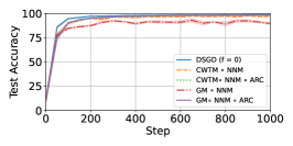
(a) $\alpha=0.5$

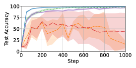
(b) $\alpha=0.1$

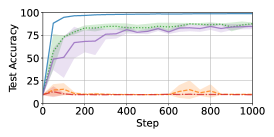
(c) extreme heterogeneity

Figure 2: Performance of Robust-DSGD when using ARC and without clipping on MNIST. Among $n=11$, we consider $f=1$ adversarial worker executing FOE [43], and vary the heterogeneity.

ARC boosts robustness in high heterogeneity. Figure 2 shows the performance of Robust-DSGD against the FOE [43] attack when using ARC opposed to no clipping with $f=1$ adversarial worker among $n=11$.When the heterogeneity is low (i.e., $\alpha=0.5$, see Figure 5), the performance of ARC and no clipping are comparable for both aggregations. When the heterogeneity increases ($\alpha=0.1$), the benefits of using ARC are more visible. CWTM $\circ$ NNM and GM $\circ$ NNM significantly struggle to learn (with a very large variance), while the same aggregations composed with ARC almost match the accuracy of DSGD towards the end of the training. In extreme heterogeneity, the improvement induced by our method is the most pronounced, as ARC enables both aggregations to reach a final accuracy close to 90%. Contrastingly, the same aggregations without clipping stagnate at an accuracy close to 10% throughout the training. Interestingly, only $f=1$ adversarial worker among $n=11$ (i.e., less than 10%) suffices to completely deteriorate the learning when no clipping is applied.

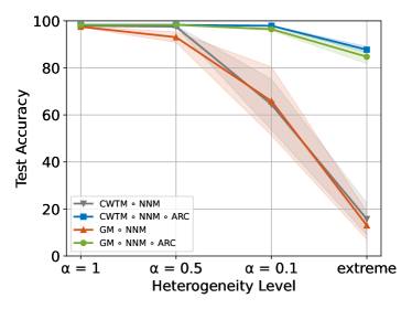
(a) $f=1$

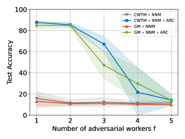
(b) extreme heterogeneity

Figure 3: Worst-case maximal accuracies achieved by Robust-DSGD, with and without ARC, on heterogeneously-distributed MNIST with $10$ honest workers. Left: $f=1$ adversarial worker among $n=11$ for varying levels of heterogeneity. Right: extreme heterogeneity for varying $f$.

Varying heterogeneity for fixed $f$. Figure 3a compares the worst-case maximal accuracies achieved by Robust-DSGD when $f=1$, with ARC and without, for varying levels of heterogeneity. While CWTM $\circ$ NNM and GM $\circ$ NNM yield comparable accuracies with ARC in low heterogeneity ($\alpha\geq 0.5$), their performance significantly degrades when $\alpha$ drops below that threshold. Indeed, when $\alpha=0.1$, their accuracies drop below 65%, while ARC enables the same aggregations to maintain their accuracy at just below 98%. In extreme heterogeneity, the performance of the aggregations without clipping completely deteriorates with accuracies close to 15%. Contrastingly, ARC efficiently mitigates the Byzantine attacks, resulting in accuracies above 85% in the worst case for both aggregations. Similar plots for $f=3,5,7$ convey similar observations (see Appendix E.1). Essentially, in settings where gradient clipping is not needed (e.g., low heterogeneity or small $f$), ARC performs at least as well as no clipping. Nonetheless, ARC induces a significant improvement near the breakdown point of SOTA robust aggregation schemes (e.g., high heterogeneity or large $f$).

	$\alpha=0.2$		$\alpha=0.075$
Aggregation	No Clipping	ARC	No Clipping	ARC
CWTM $\circ$ NNM	51.6 $\pm$ 5.1	67.8 $\pm$ 0.9	40.7 $\pm$ 0.5	60.5 $\pm$ 1.2
GM $\circ$ NNM	41.2 $\pm$ 3.5	67.0 $\pm$ 1.0	16.0 $\pm$ 2.3	60.0 $\pm$ 2.0
CWMed $\circ$ NNM	43.4 $\pm$ 4.2	69.4 $\pm$ 0.8	13.7 $\pm$ 12.1	62.7 $\pm$ 1.2
MK $\circ$ NNM	50.9 $\pm$ 5.1	68.7 $\pm$ 0.5	40.5 $\pm$ 0.7	59.9 $\pm$ 1.9

Table 1: Worst-case maximal accuracies (%) achieved by Robust-DSGD on heterogeneously-distributed CIFAR-10 with ARC and without. There is $f=1$ adversarial worker among $n=17$. As a baseline, DSGD ($f=0$) reaches 76.5% and 70% when $\alpha=0.2$ and 0.075, respectively.

SOTA robust aggregations fail in extreme heterogeneity. Figure 3b shows that for all values of $f\in\{1,...,5\}$, Robust-DSGD with CWTM $\circ$ NNM and GM $\circ$ NNM completely fails to learn, consistently yielding worst-case maximal accuracies close to 15%. This suggests that $f=1$ constitutes the breakdown point for these aggregations in extreme heterogeneity. However, composing them with ARC increases the breakdown point of these aggregations to $f=3$. Indeed, for $f=1$ and 2, ARC enables CWTM $\circ$ NNM and GM $\circ$ NNM to achieve accuracies greater than 85% in the worst case. However, when $f\geq 3$, their performance degrades, although CWTM $\circ$ NNM $\circ$ ARC reaches a satisfactory accuracy close to 70%. Moreover, even when the heterogeneity is not large, ARC still produces a significant improvement when the fraction of adversarial workers increases in the system. In Figure 1 of Section 1 where $\alpha=0.5$, the performances of ARC and no clipping are comparable for $f\leq 3$ for both aggregations.

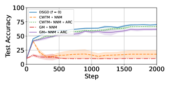
Figure 4: FOE [43] on heterogeneous CIFAR-10 with $\alpha=0.075$. $f=1$ among $n=17$.

However, when $f\geq 5$, the improvement induced by ARC is much more visible. Particularly when $f=7$, ARC enables CWTM $\circ$ NNM and GM $\circ$ NNM to reach accuracies greater than 80% in the worst case, whereas the same aggregations without clipping yield accuracies below 40%. This observation confirms the raise of the breakdown point caused by ARC to robust aggregations in practice. Plots for $\alpha=0.1$ and 1 convey the same observations (see Appendix E.1).

Improved robustness on CIFAR-10. We also conduct experiments on the more challenging CIFAR-10 task with $n=17$ and $f=1$. Table 2 shows the worst-case maximal accuracies achieved by ARC and no clipping for four robust aggregations. For $\alpha=0.2$, ARC consistently outputs accuracies greater than 67% for all aggregations, while the same aggregations without clipping yield lower accuracies (with a large variance across seeds). For instance, GM $\circ$ NNM achieves 41.2% on average, i.e., 26% less than its counterpart with ARC. In the more heterogeneous setting $\alpha=0.075$, ARC enables all aggregations to reach worst-case maximal accuracies close to 60% (with a small variance). On the contrary, executing the same methods without clipping deteriorates the performance of Robust-DSGD, with GM $\circ$ NNM and CWMed $\circ$ NNM reaching 16% and 13.7% in worst-case accuracy, respectively. This can also be seen in Figure 4, where FOE completely degrades the learning when ARC is not used, despite CWTM $\circ$ NNM reaching a peak of 40% at the start of the learning.

7 Conclusion

We have introduced a pre-aggregation clipping scheme, named adaptive robust clipping (ARC), that helps to circumvent the general limitations on the robustness to adversarial workers in distributed learning, under the standard heterogeneity model of $(G,B)$-gradient dissimilarity. We have obtained formal guarantees on the improvement in the learning error of state-of-the-art robust distributed gradient descent (Robust-DGD) when incorporating ARC. We have validated our theoretical findings through an exhaustive set of experiments on benchmark image classification tasks.

Appendix A Computational Complexity of ARC.

The algorithm starts by computing the norms of all input vectors, which takes $\mathcal{O}(nd)$ time. Note that this step is also required for static clipping. The sorting operation of the norms takes $\mathcal{O}(n\log(n))$ time. Note that if $n$ is large compared to ${k=\left\lfloor{2(f/n)(n-f)}\right\rfloor}$, one can use more efficient algorithms for finding the ${(k+1)}$-th largest element, such as quick-select [22] which has an average-case complexity of $\mathcal{O}(n)$. Finally, clipping the vectors requires $\mathcal{O}(nd)$ time. Therefore, the total complexity of ARC is $\mathcal{O}(nd+n\log(n))$. Overall, the complexity is comparable to static clipping, given that the sorting (or search) is crucially dimension independent.

Appendix B Proofs for Results in Section 4

Proofs for Lemma 4.1 and Theorem 4.2 are presented in B.1 and B.2, respectively.

Notation

Let $n\in\mathbb{N}^{*}$. Given vectors $x_{1},\ldots,x_{n}\in\mathbb{R}^{d}$ and a set $S\subseteq[n]$, we denote by $\overline{x}_{S}$ the mean of the vectors in $S$ $\overline{x}_{S}=\frac{1}{\left\lvert{S}\right\rvert}\sum_{i\in S}x_{i}$. Given a clipping parameter $C\geq 0$, let

$$y_{i}\coloneq\mathrm{clip}_{C}(x_{i})=\min\left(1,\frac{C}{\left\lVert{x_{i}}\right\rVert}\right)x_{i},$$

and

$$\overline{y}_{S}\coloneqq\frac{1}{\left\lvert{S}\right\rvert}\sum_{i\in S}y_{i}.$$

We denote by $S_{c}$ the set of clipped vectors in $S$,

$$S_{c}\coloneq\{i\in S,\left\lVert{x_{i}}\right\rVert>C\}.$$ (1)

Recall that we denote by $\mathbf{Clip}_{C}$ be the operator such that, for $x_{1},\dots,x_{n}\in\mathbb{R}^{d}$

$$\mathbf{Clip}_{C}(x_{1},\dots,x_{n}):=(\mathrm{clip}_{C}(x_{1}),\dots,\mathrm{clip}_{C}(x_{n}))\enspace.$$

Further, let $\mathbf{F}:\mathbb{R}^{n\times d}\to\mathbb{R}^{d}$. We denote by $\mathbf{F}\circ\mathbf{Clip}_{C}$ the aggregation rule that first clips the input vectors using parameter $C$, and then aggregates them using $\mathbf{F}$

$$\mathbf{F}\circ\mathbf{Clip}_{C}(x_{1},\dots,x_{n}):=\mathbf{F}(\mathbf{Clip}_{C}(x_{1},\dots,x_{n}))\enspace.$$

B.1 Proof of Lemma 4.1

See 4.1

Proof.

We use reasoning by contradiction to prove the lemma.

We first consider the case when $C>0$. Let $S\coloneqq\{1,\ldots,n-f\}$. Consider an arbitrary set of $n$ vectors $x_{1},\ldots,\,x_{n}$ in $\mathbb{R}^{d}$ such that $x_{1}=\ldots=x_{n-f}=\overline{x}_{S}$ and $\left\lVert{\overline{x}_{S}}\right\rVert=2C$. We assume that that ${\mathbf{F}\circ\mathbf{Clip}_{C}}$ is $(f,\kappa^{\prime})$-robust for some $\kappa^{\prime}\geq 0$. This assumption implies that

$$\left\lVert{\mathbf{F}\circ\mathbf{Clip}_{C}(x_{1},\ldots,x_{n})-\overline{x}_{S}}\right\rVert^{2} \leq\frac{\kappa^{\prime}}{\left\lvert{S}\right\rvert}\sum_{i\in S}\left\lVert{x_{i}-\overline{x}_{S}}\right\rVert^{2}=0.$$ (2)

Therefore,

$$\mathbf{F}\circ\mathbf{Clip}_{C}(x_{1},\ldots,x_{n})=\overline{x}_{S}.$$

However, the clipping operation results in $\mathrm{clip}_{C}(x_{1})=\ldots=\mathrm{clip}_{C}(x_{n-f})=\frac{1}{2}\overline{x}_{S}$. Therefore, by $(f,\kappa)$-robustness of $\mathbf{F}$,

$${\mathbf{F}\circ\mathbf{Clip}_{C}}(x_{1},\ldots,x_{n})=\mathbf{F}\left(\frac{1}{2}\overline{x}_{S},\ldots,\frac{1}{2}\overline{x}_{S},\mathrm{clip}_{C}(x_{n-f+1}),\ldots,\mathrm{clip}_{C}(x_{n})\right)=\frac{1}{2}\overline{x}_{S}.$$

This contradicts (2). As this contradiction holds for any value of $\kappa^{\prime}$, ${\mathbf{F}\circ\mathbf{Clip}_{C}}$ cannot be $(f,\kappa^{\prime})$-robust for any $\kappa^{\prime}$.

The proof for the case when $C=0$ is similar to the above, where we choose $x_{1}=\ldots=x_{n-f}=\overline{x}_{S}$ such that $\overline{x}_{S}$ is any vector with strictly positive norm. ∎

B.2 Proof of Theorem 4.2

Our proof relies on the following lemma, proof of which is deferred to B.2.1.

Lemma B.1.

Let $C\in\mathbb{R}^{+}$ and $\mathbf{F}$ be an $(f,\kappa)$-robust aggregation rule. Consider an arbitrary set of $n$ vectors $x_{1},x_{2},\ldots,x_{n}\in\mathbb{R}^{d}$ and an arbitrary $S\subseteq[n]$ with $\left\lvert{S}\right\rvert=n-f$. Let $S_{c}$ denote the set of indices of clipped vectors in $S$, i.e., $S_{c}\coloneqq\{i\in S,\left\lVert{x_{i}}\right\rVert>C\}$. If $\left\lvert{S\setminus S_{c}}\right\rvert\geq 1$, then

$$\left\lVert{\mathbf{F}\circ\mathbf{Clip}_{C}(x_{1},\ldots,x_{n})-\overline{x}_{S}}\right\rVert^{2}\leq\frac{\tilde{\kappa}}{\left\lvert{S}\right\rvert}\sum_{i\in S}\left\lVert{x_{i}-\overline{x}_{S}}\right\rVert^{2}\enspace,$$

where $\tilde{\kappa}=\kappa+\frac{\left\lvert{S_{c}}\right\rvert}{\left\lvert{S\setminus S_{c}}\right\rvert}$.

Lemma B.1 shows that $\mathbf{F}\circ\mathbf{Clip}_{C}$ is $(f,\tilde{\kappa})$-robust, provided that $\left\lvert{S\setminus S_{c}}\right\rvert\geq 1$ for all subsets $S$ of size $n-f$. Note that this condition is impossible to guarantee when using a fixed clipping threshold that does not depend on the input vectors. In order to ensure that $\left\lvert{S\setminus S_{c}}\right\rvert\geq 1$ for all subsets $S$ of size $n-f$, the clipping threshold $C$ should be large enough such that less than $n-f$ input vectors are clipped. By construction, ARC satisfies the condition of Lemma B.1. This brings us to the proof of Theorem 4.2, which we recall below for convenience.

See 4.2

Proof.

Since we clip the largest $\left\lfloor{2(f/n)(n-f)}\right\rfloor$ gradients, for a given $S\subseteq[n]$ with $\left\lvert{S}\right\rvert=n-f$ we have

$$\left\lvert{S_{c}}\right\rvert\leq\left\lfloor{2(f/n)(n-f)}\right\rfloor\leq 2(f/n)(n-f).$$

Therefore,

$$\left\lvert{S\setminus S_{c}}\right\rvert=\left\lvert{S}\right\rvert-\left\lvert{S_{c}}\right\rvert\geq(n-f)-\frac{2f}{n}(n-f)=(n-f)\frac{n-2f}{n}.$$

Since it is assumed that $f<n/2$, we have

$$\left\lvert{S\setminus S_{c}}\right\rvert>\left(n-\frac{n}{2}\right)\frac{n-n}{n}=0.$$

Thus, the condition $\left\lvert{S\setminus S_{c}}\right\rvert\geq 1$ is always verified. Hence, from Lemma B.1 we obtain that $\mathbf{F}\circ\mathbf{ARC}$ is $\left(f,\left(\kappa+\frac{\left\lvert{S_{c}}\right\rvert}{\left\lvert{S\setminus S_{c}}\right\rvert}\right)\right)$-robust where

$$\frac{\left\lvert{S_{c}}\right\rvert}{\left\lvert{S\setminus S_{c}}\right\rvert}\leq\frac{2(f/n)(n-f)}{(n-f)\frac{n-2f}{n}}=\frac{2f}{n-2f}.$$

This concludes the proof. ∎

B.2.1 Proof of Lemma B.1

We start by giving bounds on the variance (Lemma B.2) and the bias (Lemma B.3 and Lemma B.4) due to the clipping operation. We combine these bounds to prove the theorem.

Variance reduction due to clipping

We start by giving a bound on the variance of the clipped vectors. Recall from (1) that $S_{c}\coloneqq\{i\in S,\left\lVert{x_{i}}\right\rVert>C\}$.

Lemma B.2.

Let $C\geq 0$, $n>0$ and $f<\frac{n}{2}$. For all $S\subseteq[n]$ with $\left\lvert{S}\right\rvert=n-f$, the following holds true:

1. If $\left\lVert{\overline{x}_{S}}\right\rVert\leq C$ then

   $$\frac{1}{\left\lvert{S}\right\rvert}\sum_{i\in S}\left\lVert{y_{i}-\overline{y}_{S}}\right\rVert^{2}\leq\frac{1}{\left\lvert{S}\right\rvert}\sum_{i\in S}\left\lVert{x_{i}-\overline{x}_{S}}\right\rVert^{2}-\frac{1}{\left\lvert{S}\right\rvert}\sum_{i\in S_{c}}(\left\lVert{x_{i}}\right\rVert-C)^{2}.$$

2. If $\left\lVert{\overline{x}_{S}}\right\rVert>C$ then

   $$\frac{1}{\left\lvert{S}\right\rvert}\sum_{i\in S}\left\lVert{y_{i}-\overline{y}_{S}}\right\rVert^{2}\leq\frac{1}{\left\lvert{S}\right\rvert}\sum_{i\in S}\left\lVert{x_{i}-\overline{x}_{S}}\right\rVert^{2}-\frac{\left\lvert{S\setminus S_{c}}\right\rvert}{\left\lvert{S}\right\rvert}(\left\lVert{\overline{x}_{S}}\right\rVert-C)^{2}-\frac{1}{\left\lvert{S}\right\rvert}\sum_{i\in S_{c}}(\left\lVert{x_{i}}\right\rVert-\left\lVert{\overline{x}_{S}}\right\rVert)^{2}.$$

Proof.

Note that

$$\frac{1}{\left\lvert{S}\right\rvert}\sum_{i\in S}\left\lVert{y_{i}-\overline{y}_{S}}\right\rVert^{2} =\frac{1}{\left\lvert{S}\right\rvert}\sum_{i\in S}\left\lVert{y_{i}-\overline{x}_{S}+\overline{x}_{S}-\overline{y}_{S}}\right\rVert^{2}$$

$$=\frac{1}{\left\lvert{S}\right\rvert}\sum_{i\in S}\left(\left\lVert{y_{i}-\overline{x}_{S}}\right\rVert^{2}+\left\lVert{\overline{x}_{S}-\overline{y}_{S}}\right\rVert^{2}+2\langle y_{i}-\overline{x}_{S},\overline{x}_{S}-\overline{y}_{S}\rangle\right)$$

$$=\frac{1}{\left\lvert{S}\right\rvert}\sum_{i\in S}\left\lVert{y_{i}-\overline{x}_{S}}\right\rVert^{2}+\left\lVert{\overline{x}_{S}-\overline{y}_{S}}\right\rVert^{2}+2\left\langle\underbrace{\frac{1}{\left\lvert{S}\right\rvert}\sum_{i\in S}y_{i}}_{\overline{y}_{S}}-\overline{x}_{S},\,\overline{x}_{S}-\overline{y}_{S}\right\rangle$$

$$=\frac{1}{\left\lvert{S}\right\rvert}\sum_{i\in S}\left\lVert{y_{i}-\overline{x}_{S}}\right\rVert^{2}+\left\lVert{\overline{x}_{S}-\overline{y}_{S}}\right\rVert^{2}-2\left\langle\overline{x}_{S}-\overline{y}_{S},\,\overline{x}_{S}-\overline{y}_{S}\right\rangle$$

$$=\frac{1}{\left\lvert{S}\right\rvert}\sum_{i\in S}\left\lVert{y_{i}-\overline{x}_{S}}\right\rVert^{2}-\left\lVert{\overline{x}_{S}-\overline{y}_{S}}\right\rVert^{2}.$$ (3)

By the definition of $S_{c}$ (in (1)), for all $i\in S\setminus S_{c}$, $y_{i}=x_{i}$. Therefore,

$$\frac{1}{\left\lvert{S}\right\rvert}\sum_{i\in S}\left\lVert{y_{i}-\overline{x}_{S}}\right\rVert^{2} =\frac{1}{\left\lvert{S}\right\rvert}\sum_{i\in S\setminus S_{c}}\left\lVert{y_{i}-\overline{x}_{S}}\right\rVert^{2}+\frac{1}{\left\lvert{S}\right\rvert}\sum_{i\in S_{c}}\left\lVert{y_{i}-\overline{x}_{S}}\right\rVert^{2}$$

$$=\frac{1}{\left\lvert{S}\right\rvert}\sum_{i\in S\setminus S_{c}}\left\lVert{x_{i}-\overline{x}_{S}}\right\rVert^{2}+\frac{1}{\left\lvert{S}\right\rvert}\sum_{i\in S_{c}}\left\lVert{y_{i}-\overline{x}_{S}}\right\rVert^{2}.$$

The above can be written as

$$\frac{1}{\left\lvert{S}\right\rvert}\sum_{i\in S}\left\lVert{y_{i}-\overline{x}_{S}}\right\rVert^{2}=\frac{1}{\left\lvert{S}\right\rvert}\sum_{i\in S}\left\lVert{x_{i}-\overline{x}_{S}}\right\rVert^{2}+\frac{1}{\left\lvert{S}\right\rvert}\sum_{i\in S_{c}}(\left\lVert{y_{i}-\overline{x}_{S}}\right\rVert^{2}-\left\lVert{x_{i}-\overline{x}_{S}}\right\rVert^{2}).$$ (4)

For $i\in S_{c}$, we have $y_{i}=\frac{C}{\left\lVert{x_{i}}\right\rVert}x_{i}$. Thus, for all $i\in S_{c}$, we obtain that

$$\left\lVert{y_{i}-\overline{x}_{S}}\right\rVert^{2}-\left\lVert{x_{i}-\overline{x}_{S}}\right\rVert^{2} =\underbrace{\left\lVert{y_{i}}\right\rVert^{2}}_{=C^{2}}+\left\lVert{\overline{x}_{S}}\right\rVert^{2}-2\langle y_{i},\overline{x}_{S}\rangle-\left\lVert{x_{i}}\right\rVert^{2}-\left\lVert{\overline{x}_{S}}\right\rVert^{2}+2\langle x_{i},\overline{x}_{S}\rangle$$

$$=C^{2}-\left\lVert{x_{i}}\right\rVert^{2}+2\left(1-\frac{C}{\left\lVert{x_{i}}\right\rVert}\right)\langle x_{i},\overline{x}_{S}\rangle$$

$$=-(\left\lVert{x_{i}}\right\rVert-C)(\left\lVert{x_{i}}\right\rVert+C)+2(\left\lVert{x_{i}}\right\rVert-C)\frac{\langle x_{i},\overline{x}_{S}\rangle}{\left\lVert{x_{i}}\right\rVert}$$

$$=(\left\lVert{x_{i}}\right\rVert-C)\left(2\frac{\langle x_{i},\overline{x}_{S}\rangle}{\left\lVert{x_{i}}\right\rVert}-\left\lVert{x_{i}}\right\rVert-C\right).$$

By Cauchy-Schwarz inequality, we have $\left\langle x_{i},\,\overline{x}_{S}\right\rangle\leq\left\lVert{x_{i}}\right\rVert\left\lVert{\overline{x}_{S}}\right\rVert$ Therefore,

$$\left\lVert{y_{i}-\overline{x}_{S}}\right\rVert^{2}-\left\lVert{x_{i}-\overline{x}_{S}}\right\rVert^{2} \leq(\left\lVert{x_{i}}\right\rVert-C)\left(2\left\lVert{\overline{x}_{S}}\right\rVert-\left\lVert{x_{i}}\right\rVert-C\right).$$

Substituting from the above in (4), we obtain that

$$\frac{1}{\left\lvert{S}\right\rvert}\sum_{i\in S}\left\lVert{y_{i}-\overline{x}_{S}}\right\rVert^{2}\leq\frac{1}{\left\lvert{S}\right\rvert}\sum_{i\in S}\left\lVert{x_{i}-\overline{x}_{S}}\right\rVert^{2}+\frac{1}{\left\lvert{S}\right\rvert}\sum_{i\in S_{c}}(\left\lVert{x_{i}}\right\rVert-C)\left(2\left\lVert{\overline{x}_{S}}\right\rVert-\left\lVert{x_{i}}\right\rVert-C\right).$$

Substituting from the above in (3), we obtain that

$$\frac{1}{\left\lvert{S}\right\rvert}\sum_{i\in S}\left\lVert{y_{i}-\overline{y}_{S}}\right\rVert^{2}\leq\frac{1}{\left\lvert{S}\right\rvert}\sum_{i\in S}\left\lVert{x_{i}-\overline{x}_{S}}\right\rVert^{2}+\frac{1}{\left\lvert{S}\right\rvert}\sum_{i\in S_{c}}(\left\lVert{x_{i}}\right\rVert-C)\left(2\left\lVert{\overline{x}_{S}}\right\rVert-\left\lVert{x_{i}}\right\rVert-C\right)-\left\lVert{\overline{x}_{S}-\overline{y}_{S}}\right\rVert^{2}.$$ (5)

We now consider below the two cases: $\left\lVert{\overline{x}_{S}}\right\rVert\leq C$ and $\left\lVert{\overline{x}_{S}}\right\rVert>C$.

In the first case, i.e,. when $\left\lVert{\overline{x}_{S}}\right\rVert\leq C$, we have

$$\frac{1}{\left\lvert{S}\right\rvert}\sum_{i\in S_{c}}(\left\lVert{x_{i}}\right\rVert-C)\left(2\left\lVert{\overline{x}_{S}}\right\rVert-\left\lVert{x_{i}}\right\rVert-C\right) \leq\frac{1}{\left\lvert{S}\right\rvert}\sum_{i\in S_{c}}(\left\lVert{x_{i}}\right\rVert-C)\left(2C-\left\lVert{x_{i}}\right\rVert-C\right)$$

$$\leq-\frac{1}{\left\lvert{S}\right\rvert}\sum_{i\in S_{c}}(\left\lVert{x_{i}}\right\rVert-C)^{2}.$$

Substituting from the above in (5) yields the following

$$\frac{1}{\left\lvert{S}\right\rvert}\sum_{i\in S}\left\lVert{y_{i}-\overline{y}_{S}}\right\rVert^{2} \leq\frac{1}{\left\lvert{S}\right\rvert}\sum_{i\in S}\left\lVert{x_{i}-\overline{x}_{S}}\right\rVert^{2}-\frac{1}{\left\lvert{S}\right\rvert}\sum_{i\in S_{c}}(\left\lVert{x_{i}}\right\rVert-C)^{2}-\left\lVert{\overline{x}_{S}-\overline{y}_{S}}\right\rVert^{2}$$

$$\leq\frac{1}{\left\lvert{S}\right\rvert}\sum_{i\in S}\left\lVert{x_{i}-\overline{x}_{S}}\right\rVert^{2}-\frac{1}{\left\lvert{S}\right\rvert}\sum_{i\in S_{c}}(\left\lVert{x_{i}}\right\rVert-C)^{2}.$$

This proves the first part of the lemma.

Consider the second case, i.e., $\left\lVert{\overline{x}_{S}}\right\rVert>C$. Note that

$$\frac{1}{\left\lvert{S}\right\rvert}\sum_{i\in S_{c}}(\left\lVert{x_{i}}\right\rVert-C)\left(2\left\lVert{\overline{x}_{S}}\right\rVert-\left\lVert{x_{i}}\right\rVert-C\right) =\frac{1}{\left\lvert{S}\right\rvert}\sum_{i\in S_{c}}\left((\left\lVert{\overline{x}_{S}}\right\rVert-C)^{2}-(\left\lVert{x_{i}}\right\rVert-\left\lVert{\overline{x}_{S}}\right\rVert)^{2}\right)$$

$$=\frac{\left\lvert{S_{c}}\right\rvert}{\left\lvert{S}\right\rvert}(\left\lVert{\overline{x}_{S}}\right\rVert-C)^{2}-\frac{1}{\left\lvert{S}\right\rvert}\sum_{i\in S_{c}}(\left\lVert{x_{i}}\right\rVert-\left\lVert{\overline{x}_{S}}\right\rVert)^{2}.$$ (6)

Since $\left\lVert{\overline{x}_{S}}\right\rVert>C$, and $\left\lVert{\overline{y}_{S}}\right\rVert\leq C$, we have $\left\lVert{\overline{x}_{S}}\right\rVert-\left\lVert{\overline{y}_{S}}\right\rVert\geq\left\lVert{\overline{x}_{S}}\right\rVert-C\geq 0$ . This, in conjunction with the reverse triangle inequality, implies that

$$\left\lVert{\overline{x}_{S}-\overline{y}_{S}}\right\rVert^{2}\geq\left(\left\lVert{\overline{x}_{S}}\right\rVert-\left\lVert{\overline{y}_{S}}\right\rVert\right)^{2}\geq(\left\lVert{\overline{x}_{S}}\right\rVert-C)^{2}.$$ (7)

Substituting from (6) and (7) in (5) yields the following:

$$\frac{1}{\left\lvert{S}\right\rvert}\sum_{i\in S}\left\lVert{y_{i}-\overline{y}_{S}}\right\rVert^{2} \leq\frac{1}{\left\lvert{S}\right\rvert}\sum_{i\in S}\left\lVert{x_{i}-\overline{x}_{S}}\right\rVert^{2}+\frac{\left\lvert{S_{c}}\right\rvert}{\left\lvert{S}\right\rvert}(\left\lVert{\overline{x}_{S}}\right\rVert-C)^{2}-\frac{1}{\left\lvert{S}\right\rvert}\sum_{i\in S_{c}}(\left\lVert{x_{i}}\right\rVert-\left\lVert{\overline{x}_{S}}\right\rVert)^{2}-(\left\lVert{\overline{x}_{S}}\right\rVert-C)^{2}$$

$$\leq\frac{1}{\left\lvert{S}\right\rvert}\sum_{i\in S}\left\lVert{x_{i}-\overline{x}_{S}}\right\rVert^{2}+\left(\frac{\left\lvert{S_{c}}\right\rvert}{\left\lvert{S}\right\rvert}-1\right)(\left\lVert{\overline{x}_{S}}\right\rVert-C)^{2}-\frac{1}{\left\lvert{S}\right\rvert}\sum_{i\in S_{c}}(\left\lVert{x_{i}}\right\rVert-\left\lVert{\overline{x}_{S}}\right\rVert)^{2}$$

$$=\frac{1}{\left\lvert{S}\right\rvert}\sum_{i\in S}\left\lVert{x_{i}-\overline{x}_{S}}\right\rVert^{2}-\frac{\left\lvert{S\setminus S_{c}}\right\rvert}{\left\lvert{S}\right\rvert}(\left\lVert{\overline{x}_{S}}\right\rVert-C)^{2}-\frac{1}{\left\lvert{S}\right\rvert}\sum_{i\in S_{c}}(\left\lVert{x_{i}}\right\rVert-\left\lVert{\overline{x}_{S}}\right\rVert)^{2}.$$

This proves the second part, which concludes the proof of the lemma. ∎

Bias due to clipping

We now bound the bias induced by clipping the input vectors.

Lemma B.3.

Let $C\geq 0$, $n>0$, $f<\frac{n}{2}$, and $S\subseteq[n]$, $\left\lvert{S}\right\rvert=n-f$. Then,

$$\left\lVert{\overline{x}_{S}-\overline{y}_{S}}\right\rVert^{2} \leq\frac{\left\lvert{S_{c}}\right\rvert}{\left\lvert{S}\right\rvert^{2}}\sum_{i\in S_{c}}(\left\lVert{x_{i}}\right\rVert-C)^{2}.$$

Proof.

Note that

$$\left\lVert{\overline{x}_{S}-\overline{y}_{S}}\right\rVert^{2} =\left\lVert{\frac{1}{\left\lvert{S}\right\rvert}\sum_{i\in S}x_{i}-\frac{1}{\left\lvert{S}\right\rvert}\sum_{i\in S}y_{i}}\right\rVert^{2}=\left\lVert{\frac{1}{\left\lvert{S}\right\rvert}\sum_{i\in S}(x_{i}-y_{i})}\right\rVert^{2}.$$

As $x_{i}=y_{i}$ for all $i\in S\setminus S_{c}$, we have

$$\left\lVert{\overline{x}_{S}-\overline{y}_{S}}\right\rVert^{2} =\frac{1}{\left\lvert{S}\right\rvert^{2}}\left\lVert{\sum_{i\in S_{c}}(x_{i}-y_{i})}\right\rVert^{2}.$$

Due to Jensen’s inequality,

$$\left\lVert{\overline{x}_{S}-\overline{y}_{S}}\right\rVert^{2} =\frac{\left\lvert{S_{c}}\right\rvert^{2}}{\left\lvert{S}\right\rvert^{2}}\left\lVert{\frac{1}{\left\lvert{S_{c}}\right\rvert}\sum_{i\in S_{c}}(x_{i}-y_{i})}\right\rVert^{2}\leq\frac{\left\lvert{S_{c}}\right\rvert}{\left\lvert{S}\right\rvert^{2}}\sum_{i\in S_{c}}\left\lVert{x_{i}-y_{i}}\right\rVert^{2}.$$

As $y_{i}=\frac{C}{\left\lVert{x_{i}}\right\rVert}x_{i}$ for all $i\in S_{c}$, substituting this in the above proves the lemma. ∎

We now show that the bias is upper bounded by a multiplicative factor of the variance of the input vectors, as long as there is at least one unclipped honest vector.

Lemma B.4 (Bias due to clipping).

$C\geq 0$, $n>0$, $f<\nicefrac{{n}}{{2}}$, and $S\subseteq[n]$, $\left\lvert{S}\right\rvert=n-f$, if $\left\lvert{S\setminus S_{c}}\right\rvert\geq 1$ then

$$\left\lVert{\overline{x}_{S}-\overline{y}_{S}}\right\rVert^{2}\leq\frac{\left\lvert{S_{c}}\right\rvert}{\left\lvert{S\setminus S_{c}}\right\rvert}\frac{1}{\left\lvert{S}\right\rvert}\sum_{i\in S}\left\lVert{x_{i}-\overline{x}_{S}}\right\rVert^{2}.$$

Proof.

We assume throughout the proof that $\left\lvert{S_{c}}\right\rvert>0$. Otherwise, if $\left\lvert{S_{c}}\right\rvert=0$, the bias is $0$ and the statement is trivially true.

By Lemma B.3, we have

$$\left\lVert{\overline{x}_{S}-\overline{y}_{S}}\right\rVert^{2} \leq\frac{\left\lvert{S_{c}}\right\rvert}{\left\lvert{S}\right\rvert^{2}}\sum_{i\in S_{c}}(\left\lVert{x_{i}}\right\rVert-C)^{2}.$$ (8)

We distinguish two cases: $\left\lVert{\overline{x}_{S}}\right\rVert\leq C$ and $\left\lVert{\overline{x}_{S}}\right\rVert>C$. In the first case we have that

$$0\leq\left\lVert{x_{i}}\right\rVert-C\leq\left\lVert{x_{i}}\right\rVert-\left\lVert{\overline{x}_{S}}\right\rVert.$$

Substituting the above in (8), we find

$$\left\lVert{\overline{x}_{S}-\overline{y}_{S}}\right\rVert^{2}\leq\frac{\left\lvert{S_{c}}\right\rvert}{\left\lvert{S}\right\rvert^{2}}\sum_{i\in S_{c}}(\left\lVert{x_{i}}\right\rVert-\left\lVert{\overline{x}_{S}}\right\rVert)^{2}\leq\frac{\left\lvert{S_{c}}\right\rvert}{\left\lvert{S}\right\rvert^{2}}\sum_{i\in S}(\left\lVert{x_{i}}\right\rVert-\left\lVert{\overline{x}_{S}}\right\rVert)^{2}.$$

Using the reverse triangle inequality, we have that $(\left\lVert{x_{i}}\right\rVert-\left\lVert{\overline{x}_{S}}\right\rVert)^{2}\leq\left\lVert{x_{i}-\overline{x}_{S}}\right\rVert^{2}$. This implies that

$$\left\lVert{\overline{x}_{S}-\overline{y}_{S}}\right\rVert^{2}\leq\frac{\left\lvert{S_{c}}\right\rvert}{\left\lvert{S}\right\rvert^{2}}\sum_{i\in S}(\left\lVert{x_{i}}\right\rVert-\left\lVert{\overline{x}_{S}}\right\rVert)^{2}\leq\frac{\left\lvert{S_{c}}\right\rvert}{\left\lvert{S\setminus S_{c}}\right\rvert}\frac{1}{\left\lvert{S}\right\rvert}\sum_{i\in S}\left\lVert{x_{i}-\overline{x}_{S}}\right\rVert^{2}.$$

This proves the result for the first case.

Consider now the second case, i.e $\left\lVert{\overline{x}_{S}}\right\rVert>C$. Noting that we assume that $\left\lvert{S\setminus S_{c}}\right\rvert\geq 1$ and using Young’s inequality with $c=\frac{\left\lvert{S_{c}}\right\rvert}{\left\lvert{S\setminus S_{c}}\right\rvert}$, we find, for any $i\in S_{c}$,

$$(\left\lVert{x_{i}}\right\rVert-C)^{2} =(\left\lVert{x_{i}}\right\rVert-\left\lVert{\overline{x}_{S}}\right\rVert+\left\lVert{\overline{x}_{S}}\right\rVert-C)^{2}$$

$$\leq(1+c)(\left\lVert{x_{i}}\right\rVert-\left\lVert{\overline{x}_{S}}\right\rVert)^{2}+(1+1/c)(\left\lVert{\overline{x}_{S}}\right\rVert-C)^{2})$$

$$=\frac{\left\lvert{S_{c}}\right\rvert+\left\lvert{S\setminus S_{c}}\right\rvert}{\left\lvert{S\setminus S_{c}}\right\rvert}(\left\lVert{x_{i}}\right\rVert-\left\lVert{\overline{x}_{S}}\right\rVert)^{2}+\frac{\left\lvert{S_{c}}\right\rvert+\left\lvert{S\setminus S_{c}}\right\rvert}{\left\lvert{S_{c}}\right\rvert}(\left\lVert{\overline{x}_{S}}\right\rVert-C)^{2}.$$

Recall from (1) that $S_{c}\coloneqq\{i\in S,\left\lVert{x_{i}}\right\rVert>C\}$. This implies that $\left\lvert{S_{c}}\right\rvert+\left\lvert{S\setminus S_{c}}\right\rvert=\left\lvert{S}\right\rvert$. Therefore

$$(\left\lVert{x_{i}}\right\rVert-C)^{2} \leq\left\lvert{S}\right\rvert\left(\frac{1}{\left\lvert{S\setminus S_{c}}\right\rvert}(\left\lVert{x_{i}}\right\rVert-\left\lVert{\overline{x}_{S}}\right\rVert)^{2}+\frac{1}{\left\lvert{S_{c}}\right\rvert}(\left\lVert{\overline{x}_{S}}\right\rVert-C)^{2}\right).$$ (9)

Substituting (9) in (8), we find

$$\left\lVert{\overline{x}_{S}-\overline{y}_{S}}\right\rVert^{2} \leq\frac{\left\lvert{S_{c}}\right\rvert}{\left\lvert{S}\right\rvert^{2}}\sum_{i\in S_{c}}\left\lvert{S}\right\rvert\left(\frac{1}{\left\lvert{S\setminus S_{c}}\right\rvert}(\left\lVert{x_{i}}\right\rVert-\left\lVert{\overline{x}_{S}}\right\rVert)^{2}+\frac{1}{\left\lvert{S_{c}}\right\rvert}(\left\lVert{\overline{x}_{S}}\right\rVert-C)^{2}\right)$$

$$=\frac{\left\lvert{S_{c}}\right\rvert}{\left\lvert{S}\right\rvert}\left(\frac{1}{\left\lvert{S\setminus S_{c}}\right\rvert}\sum_{i\in S_{c}}(\left\lVert{x_{i}}\right\rVert-\left\lVert{\overline{x}_{S}}\right\rVert)^{2}+(\left\lVert{\overline{x}_{S}}\right\rVert-C)^{2}\right).$$ (10)

Since $\left\lVert{\overline{x}_{S}}\right\rVert>C$, we have for any $i\in S\setminus S_{c}$

$$0\leq\left\lVert{\overline{x}_{S}}\right\rVert-C\leq\left\lVert{\overline{x}_{S}}\right\rVert-\left\lVert{x_{i}}\right\rVert.$$

Therefore

$$\left\lvert{S\setminus S_{c}}\right\rvert(\left\lVert{\overline{x}_{S}}\right\rVert-C)^{2} \leq\sum_{i\in S\setminus S_{c}}(\left\lVert{\overline{x}_{S}}\right\rVert-\left\lVert{x_{i}}\right\rVert)^{2}$$

Which gives the bound

$$(\left\lVert{\overline{x}_{S}}\right\rVert-C)^{2} \leq\frac{1}{\left\lvert{S\setminus S_{c}}\right\rvert}\sum_{i\in S\setminus S_{c}}(\left\lVert{\overline{x}_{S}}\right\rVert-\left\lVert{x_{i}}\right\rVert)^{2}.$$ (11)

Substituting (11) in (10), we find

$$\left\lVert{\overline{x}_{S}-\overline{y}_{S}}\right\rVert^{2} \leq\frac{\left\lvert{S_{c}}\right\rvert}{\left\lvert{S}\right\rvert}\left(\frac{1}{\left\lvert{S\setminus S_{c}}\right\rvert}\sum_{i\in S_{c}}(\left\lVert{x_{i}}\right\rVert-\left\lVert{\overline{x}_{S}}\right\rVert)^{2}+\frac{1}{\left\lvert{S\setminus S_{c}}\right\rvert}\sum_{i\in S\setminus S_{c}}(\left\lVert{x_{i}}\right\rVert-\left\lVert{\overline{x}_{S}}\right\rVert)^{2}\right)$$

$$=\frac{\left\lvert{S_{c}}\right\rvert}{\left\lvert{S\setminus S_{c}}\right\rvert}\frac{1}{\left\lvert{S}\right\rvert}\sum_{i\in S}(\left\lVert{x_{i}}\right\rVert-\left\lVert{\overline{x}_{S}}\right\rVert)^{2}\leq\frac{\left\lvert{S_{c}}\right\rvert}{\left\lvert{S\setminus S_{c}}\right\rvert}\frac{1}{\left\lvert{S}\right\rvert}\sum_{i\in S}\left\lVert{x_{i}-\overline{x}_{S}}\right\rVert^{2}.$$

This proves the result for the second case and concludes the proof. ∎

Proof of LemmaB.1

Let us recall the lemma below.

See B.1

Proof.

We assume throughout the proof that $\left\lvert{S_{c}}\right\rvert>0$. Otherwise, the statement is trivially true by $(f,\kappa)$-robustness of $\mathbf{F}$ and the fact that the vectors in $S$ remain unchanged after the clipping operation.

Consider first the case $\kappa=0$. Since $\kappa\geq\frac{f}{n-2f}$ , we have that $f=0$. Recall that we denote $y_{i}\coloneq\mathrm{clip}_{C}(x_{i})$ and $\overline{y}_{S}\coloneqq\frac{1}{\left\lvert{S}\right\rvert}\sum_{i\in S}y_{i}$. Since $\kappa=0$, the output of $\mathbf{F}$ will correspond to the average of its input, which implies that

$$\left\lVert{\mathbf{F}\circ\mathbf{Clip}_{C}(x_{1},\ldots,x_{n})-\overline{y}_{S}}\right\rVert^{2}=\left\lVert{\mathbf{F}(y_{1},\ldots,y_{n})-\overline{y}_{S}}\right\rVert^{2}=0.$$

Therefore

$$\mathbf{F}\circ\mathbf{Clip}_{C}(x_{1},\ldots,x_{n})=\overline{y}_{S}.$$

We find then

$$\left\lVert{\mathbf{F}\circ\mathbf{Clip}_{C}(x_{1},\ldots,x_{n})-\overline{x}_{S}}\right\rVert^{2}=\left\lVert{\overline{y}_{S}-\overline{x}_{S}}\right\rVert^{2}.$$

The result for the case $\kappa=0$ follows from lemma B.4.

Suppose now that $\kappa>0$. Using Young’s inequality with $c=\frac{\left\lvert{S_{c}}\right\rvert}{\kappa\left\lvert{S\setminus S_{c}}\right\rvert}$ we find

$$\left\lVert{\mathbf{F}\circ\mathbf{Clip}_{C}(x_{1},\ldots,x_{n})-\overline{x}_{S}}\right\rVert^{2} =\left\lVert{\mathbf{F}\circ\mathbf{Clip}_{C}(x_{1},\ldots,x_{n})-\overline{y}_{S}+\overline{y}_{S}-\overline{x}_{S}}\right\rVert^{2}$$

$$\leq\left(1+c\right)\left\lVert{\mathbf{F}\circ\mathbf{Clip}_{C}(x_{1},\ldots,x_{n})-\overline{y}_{S}}\right\rVert^{2}+\left(1+\frac{1}{c}\right)\left\lVert{\overline{x}_{S}-\overline{y}_{S}}\right\rVert^{2}.$$ (12)

On the one hand, by $(f,\kappa)$-robustness of $\mathbf{F}$, we have

$$(1+c)\left\lVert{\mathbf{F}\circ\mathbf{Clip}_{C}(x_{1},\ldots,x_{n})-\overline{y}_{S}}\right\rVert^{2} =(1+c)\left\lVert{\mathbf{F}(y_{1},\ldots,y_{n})-\overline{y}_{S}}\right\rVert^{2}$$

$$\leq(1+c)\frac{\kappa}{\left\lvert{S}\right\rvert}\sum_{i\in S}\left\lVert{y_{i}-\overline{y}_{S}}\right\rVert^{2}$$

$$=\left(\kappa+\frac{\left\lvert{S_{c}}\right\rvert}{\left\lvert{S\setminus S_{c}}\right\rvert}\right)\frac{1}{\left\lvert{S}\right\rvert}\sum_{i\in S}\left\lVert{y_{i}-\overline{y}_{S}}\right\rVert^{2}.$$ (13)

On the other hand, we have

$$(1+\nicefrac{{1}}{{c}})\left\lVert{\overline{x}_{S}-\overline{y}_{S}}\right\rVert^{2}=\left(1+\frac{\kappa\left\lvert{S\setminus S_{c}}\right\rvert}{\left\lvert{S_{c}}\right\rvert}\right)\left\lVert{\overline{x}_{S}-\overline{y}_{S}}\right\rVert^{2}=\left(\kappa+\frac{\left\lvert{S_{c}}\right\rvert}{\left\lvert{S\setminus S_{c}}\right\rvert}\right)\frac{\left\lvert{S\setminus S_{c}}\right\rvert}{\left\lvert{S_{c}}\right\rvert}\left\lVert{\overline{x}_{S}-\overline{y}_{S}}\right\rVert^{2}.$$ (14)

Substituting (13) and (14) in (12) we obtain that

$$\left\lVert{\mathbf{F}\circ\mathbf{Clip}_{C}(x_{1},\ldots,x_{n})-\overline{x}_{S}}\right\rVert^{2} \leq\left(\kappa+\frac{\left\lvert{S_{c}}\right\rvert}{\left\lvert{S\setminus S_{c}}\right\rvert}\right)\left(\frac{1}{\left\lvert{S}\right\rvert}\sum_{i\in S}\left\lVert{y_{i}-\overline{y}_{S}}\right\rVert^{2}+\frac{\left\lvert{S\setminus S_{c}}\right\rvert}{\left\lvert{S_{c}}\right\rvert}\left\lVert{\overline{x}_{S}-\overline{y}_{S}}\right\rVert^{2}\right).$$ (15)

We consider below the two cases $\left\lVert{\overline{x}_{S}}\right\rVert\leq C$ and $\left\lVert{\overline{x}_{S}}\right\rVert>C$ separately.

In the first case, we use the the first part of lemma B.2 and lemma B.3 to obtain that

$$\frac{1}{\left\lvert{S}\right\rvert}\sum_{i\in S}\left\lVert{y_{i}-\overline{y}_{S}}\right\rVert^{2}+\frac{\left\lvert{S\setminus S_{c}}\right\rvert}{\left\lvert{S}\right\rvert}\left\lVert{\overline{x}_{S}-\overline{y}_{S}}\right\rVert^{2}$$

$$\leq\frac{1}{\left\lvert{S}\right\rvert}\sum_{i\in S}\left\lVert{x_{i}-\overline{x}_{S}}\right\rVert^{2}-\frac{1}{\left\lvert{S}\right\rvert}\sum_{i\in S_{c}}(\left\lVert{x_{i}}\right\rVert-C)^{2}+\frac{\left\lvert{S\setminus S_{c}}\right\rvert}{\left\lvert{S}\right\rvert}\frac{1}{\left\lvert{S}\right\rvert}\sum_{i\in S_{c}}(\left\lVert{x_{i}}\right\rVert-C)^{2}$$

$$=\frac{1}{\left\lvert{S}\right\rvert}\sum_{i\in S}\left\lVert{x_{i}-\overline{x}_{S}}\right\rVert^{2}-\frac{\left\lvert{S_{c}}\right\rvert}{\left\lvert{S}\right\rvert}\frac{1}{\left\lvert{S}\right\rvert}\sum_{i\in S}(\left\lVert{x_{i}}\right\rVert-C)^{2}\leq\frac{1}{\left\lvert{S}\right\rvert}\sum_{i\in S}\left\lVert{x_{i}-\overline{x}_{S}}\right\rVert^{2}.$$

This proves the result for this case.

Consider the second case, i.e $\left\lVert{\overline{x}_{S}}\right\rVert>C$. Following the proof of corollary B.4 until (10) we have

$$\left\lVert{\overline{x}_{S}-\overline{y}_{S}}\right\rVert^{2}\leq\frac{\left\lvert{S_{c}}\right\rvert}{\left\lvert{S}\right\rvert}\left(\frac{1}{\left\lvert{S\setminus S_{c}}\right\rvert}\sum_{i\in S_{c}}(\left\lVert{x_{i}}\right\rVert-\left\lVert{\overline{x}_{S}}\right\rVert)^{2}+(\left\lVert{\overline{x}_{S}}\right\rVert-C)^{2}\right).$$

Therefore,

$$\frac{\left\lvert{S\setminus S_{c}}\right\rvert}{\left\lvert{S_{c}}\right\rvert}\left\lVert{\overline{x}_{S}-\overline{y}_{S}}\right\rVert^{2} \leq\frac{\left\lvert{S\setminus S_{c}}\right\rvert}{\left\lvert{S}\right\rvert}\left(\frac{1}{\left\lvert{S\setminus S_{c}}\right\rvert}\sum_{i\in S_{c}}(\left\lVert{x_{i}}\right\rVert-\left\lVert{\overline{x}_{S}}\right\rVert)^{2}+(\left\lVert{\overline{x}_{S}}\right\rVert-C)^{2}\right)$$

$$\leq\frac{1}{\left\lvert{S}\right\rvert}\sum_{i\in S_{c}}(\left\lVert{x_{i}}\right\rVert-\left\lVert{\overline{x}_{S}}\right\rVert)^{2}+\frac{\left\lvert{S\setminus S_{c}}\right\rvert}{\left\lvert{S}\right\rvert}(\left\lVert{\overline{x}_{S}}\right\rVert-C)^{2}.$$

Using the above in conjunction with lemma B.2 for the case $\left\lVert{\overline{x}_{S}}\right\rVert>C$ in (15) proves the result for the second case, which concludes the proof. ∎

Appendix C Proofs for Results in Section 5

Proofs for Theorem 5.1, Corollary 5.2, Theorem 5.4 and Corollary 5.5 are presented in appendices C.2, C.3, C.4 and C.5, respectively.

C.1 Assuming $\left\lVert{\mathbf{F}\left(x_{1},\ldots,x_{n}\right)}\right\rVert\leq\max_{i\in[n]}\left\lVert{x_{i}}\right\rVert$ is Without Loss of Generality

Recall that we assume $\left\lVert{\mathbf{F}\left(x_{1},\ldots,x_{n}\right)}\right\rVert\leq\max_{i\in[n]}\left\lVert{x_{i}}\right\rVert$ for all set of $n$ vectors $x_{1},\ldots,x_{n}\in\mathbb{R}^{d}$. In case this is not true, we can instead use the aggregation rule $\mathbf{F}^{\dagger}$ given by

$$\mathbf{F}^{\dagger}\left(x_{1},\ldots,x_{n}\right)\coloneqq\mathrm{clip}_{C}\left(\mathbf{F}\left(x_{1},\ldots,x_{n}\right)\right),~{}\text{where}~{}C=\max_{i\in[n]}\left\lVert{x_{i}}\right\rVert.$$

This modification to the aggregation rule does not affect the learning guarantee. Specifically, due to the non-expansion property of $\mathrm{clip}_{C}(\cdot)$, for any non-empty set $S\subseteq[n]$, we have

$$\left\lVert{\mathbf{F}^{\dagger}\left(x_{1},\ldots,x_{n}\right)-\overline{x}_{S}}\right\rVert\leq\left\lVert{\mathbf{F}\left(x_{1},\ldots,x_{n}\right)-\overline{x}_{S}}\right\rVert,$$

where $\overline{x}_{S}\coloneqq\frac{1}{\left\lvert{S}\right\rvert}\sum\limits_{i\in S}x_{i}$. Thus, if $\mathbf{F}$ is $(f,\kappa)$-robust, then $\mathbf{F}^{\dagger}$ is also $(f,\kappa)$-robust. Hence, we can make the above assumption on $\left\lVert{\mathbf{F}\left(x_{1},\ldots,x_{n}\right)}\right\rVert$ without loss of generality.

C.2 Proof of Theorem 5.1

Our proof relies on the following lemma.

Lemma C.1.

For all $t\in[T]$, we obtain that

$$\max_{i\in\mathcal{H}}\left\lVert{\nabla\mathcal{L}_{i}({{\theta}_{t}})}\right\rVert\leq\exp{\left(\gamma LT\right)}~{}\max_{i\in\mathcal{H}}\left\lVert{\nabla\mathcal{L}_{i}({{\theta}_{1}})}\right\rVert.$$

Proof.

Consider an arbitrary $t\in[T]$. Let $(x_{1},\ldots,\,x_{n})\coloneqq\mathbf{ARC}\left({{g}^{\left({1}\right)}_{t}},\ldots,~{}{{g}^{\left({n}\right)}_{t}}\right)$. As $n>2f$ and $\left\lvert{\mathcal{H}}\right\rvert=n-f$, the clipping threshold $C$ used in ARC (see Algorithm 2) is bounded by $\max_{i\in\mathcal{H}}\left\lVert{{{g}^{\left({i}\right)}_{t}}}\right\rVert$. Therefore,

$$\max_{i\in[n]}\left\lVert{x_{i}}\right\rVert\leq\max_{i\in\mathcal{H}}\left\lVert{{{g}^{\left({i}\right)}_{t}}}\right\rVert=\max_{i\in\mathcal{H}}\left\lVert{\nabla\mathcal{L}_{i}({{\theta}_{t}})}\right\rVert.$$ (16)

Since we assume (without loss of generality) that, for any set of $n$ vectors $z_{1},\ldots,z_{n}\in\mathbb{R}^{d}$, $\left\lVert{\mathbf{F}\left(z_{1},\ldots,z_{n}\right)}\right\rVert\leq\max_{i\in[n]}\left\lVert{z_{i}}\right\rVert$ (see the discussion in Section 5.1), from (16) we obtain that

$$\left\lVert{R_{t}}\right\rVert=\left\lVert{\mathbf{F}\circ\mathbf{ARC}\left({{g}^{\left({1}\right)}_{t}},\ldots,~{}{{g}^{\left({n}\right)}_{t}}\right)}\right\rVert\leq\max_{i\in[n]}\left\lVert{x_{i}}\right\rVert\leq\max_{i\in\mathcal{H}}\left\lVert{\nabla\mathcal{L}_{i}({{\theta}_{t}})}\right\rVert.$$

Recall that ${{\theta}_{t+1}}\coloneqq{{\theta}_{t}}-\gamma R_{t}$. Thus, from above we obtain that

$$\left\lVert{{{\theta}_{t+1}}-{{\theta}_{t}}}\right\rVert\leq\gamma~{}\max_{i\in\mathcal{H}}\left\lVert{\nabla\mathcal{L}_{i}({{\theta}_{t}})}\right\rVert.$$ (17)

Due to $L$-Lipschitz smoothness of $\mathcal{L}_{i}({{\theta}})$ for all $i\in\mathcal{H}$, the above implies that

$$\left\lVert{\nabla\mathcal{L}_{i}({{\theta}_{t+1}})-\nabla\mathcal{L}_{i}({{\theta}_{t}})}\right\rVert\leq\gamma L~{}\max_{i\in\mathcal{H}}\left\lVert{\nabla\mathcal{L}_{i}({{\theta}_{t}})}\right\rVert,\quad\forall i\in\mathcal{H}.$$

This, in conjunction with the triangle inequality, implies that

$$\left\lVert{\nabla\mathcal{L}_{i}({{\theta}_{t+1}})}\right\rVert\leq\left\lVert{\nabla\mathcal{L}_{i}({{\theta}_{t}})}\right\rVert+\gamma L~{}\max_{i\in\mathcal{H}}\left\lVert{\nabla\mathcal{L}_{i}({{\theta}_{t}})}\right\rVert,\quad\forall i\in\mathcal{H}.$$

Therefore,

$$\max_{i\in\mathcal{H}}\left\lVert{\nabla\mathcal{L}_{i}({{\theta}_{t+1}})}\right\rVert\leq\max_{i\in\mathcal{H}}\left\lVert{\nabla\mathcal{L}_{i}({{\theta}_{t}})}\right\rVert+\gamma L\max_{i\in\mathcal{H}}~{}\left\lVert{\nabla\mathcal{L}_{i}({{\theta}_{t}})}\right\rVert=\left(1+\gamma L\right)\max_{i\in\mathcal{H}}~{}\left\lVert{\nabla\mathcal{L}_{i}({{\theta}_{t}})}\right\rVert.$$

As $t$ was chosen arbitrarily from $[T]$, the above holds true for all $t\in[T]$. For an arbitrary $\tau\in[T]$, using the inequality recursively for $t=\tau,\ldots,1$ we obtain that

$$\max_{i\in\mathcal{H}}\left\lVert{\nabla\mathcal{L}_{i}({{\theta}_{\tau+1}})}\right\rVert\leq\left(1+\gamma L\right)^{\tau}\max_{i\in\mathcal{H}}~{}\left\lVert{\nabla\mathcal{L}_{i}({{\theta}_{1}})}\right\rVert\leq\left(1+\gamma L\right)^{T}\max_{i\in\mathcal{H}}~{}\left\lVert{\nabla\mathcal{L}_{i}({{\theta}_{1}})}\right\rVert.$$

Since $\left(1+\gamma L\right)^{T}\leq\exp{(\gamma LT)}$, the above concludes the proof. ∎

We are now ready to present our proof of Theorem 5.1, recalled below.

See 5.1

Proof.

For simplicity, we write $\mathcal{L}_{\mathcal{H}}$ as $\mathcal{L}$ throughout the proof.

Consider an arbitrary $t\in[T]$. Due to $L$-Lipschitz smoothness of $\mathcal{L}({{\theta}_{)}}$, we obtain that

$$\mathcal{L}({{\theta}_{t+1}})\leq\mathcal{L}({{\theta}_{t}})+\left\langle{{\theta}_{t+1}}-{{\theta}_{t}},\,\nabla\mathcal{L}({{{\theta}_{t}}})\right\rangle+\frac{L}{2}\left\lVert{{{\theta}_{t+1}}-{{\theta}_{t}}}\right\rVert^{2}.$$

Substituting ${{\theta}_{t+1}}={{\theta}_{t}}-\gamma R_{t}$, and using the identity: $2\left\langle a,\,b\right\rangle=\left\lVert{a}\right\rVert^{2}+\left\lVert{b}\right\rVert^{2}-\left\lVert{a-b}\right\rVert^{2}$, we obtain that

$$\mathcal{L}({{\theta}_{t+1}})\leq\mathcal{L}({{\theta}_{t}})-\frac{\gamma}{2}\left\lVert{\nabla\mathcal{L}({{\theta}_{t}})}\right\rVert^{2}+\frac{\gamma}{2}\left\lVert{R_{t}-\nabla\mathcal{L}({{\theta}_{t}})}\right\rVert^{2}-\frac{\gamma}{2}\left(1-\gamma L\right)\left\lVert{R_{t}}\right\rVert^{2}.$$

Since $\gamma\leq\frac{1}{L}$, $\left(1-\gamma L\right)\geq 0$. Therefore, from above we obtain that

$$\mathcal{L}({{\theta}_{t+1}})\leq\mathcal{L}({{\theta}_{t}})-\frac{\gamma}{2}\left\lVert{\nabla\mathcal{L}({{\theta}_{t}})}\right\rVert^{2}+\frac{\gamma}{2}\left\lVert{R_{t}-\nabla\mathcal{L}({{\theta}_{t}})}\right\rVert^{2}.$$

Recall that $t$ is chosen arbitrarily from $[T]$. Thus, the above holds true for all $t\in[T]$. Taking summation on both sides from $t=1$ to $t=T$ we obtain that

$$\frac{\gamma}{2}\sum_{t=1}^{T}\left\lVert{\nabla\mathcal{L}({{\theta}_{t}})}\right\rVert^{2}\leq\mathcal{L}({{\theta}_{t}})-\mathcal{L}({{\theta}_{T+1}})+\frac{\gamma}{2}\sum_{t=1}^{T}\left\lVert{R_{t}-\nabla\mathcal{L}({{\theta}_{t}})}\right\rVert^{2}.$$

Multiplying both sides by $2/(\gamma T)$ we obtain that

$$\frac{1}{T}\sum_{t=1}^{T}\left\lVert{\nabla\mathcal{L}({{\theta}_{t}})}\right\rVert^{2}\leq\frac{2\left(\mathcal{L}({{\theta}_{1}})-\mathcal{L}({{\theta}_{T+1}})\right)}{\gamma T}+\frac{1}{T}\sum_{t=1}^{T}\left\lVert{R_{t}-\nabla\mathcal{L}({{\theta}_{t}})}\right\rVert^{2}.$$

Note that $\mathcal{L}({{\theta}_{1}})-\mathcal{L}({{\theta}_{T+1}})=\mathcal{L}({{\theta}_{1}})-\mathcal{L}^{*}-\left(\mathcal{L}({{\theta}_{T+1}})-\mathcal{L}^{*}\right)\leq\mathcal{L}({{\theta}_{1}})-\mathcal{L}^{*}\leq\Delta_{o}$. Using this above we obtain that

$$\frac{1}{T}\sum_{t=1}^{T}\left\lVert{\nabla\mathcal{L}({{\theta}_{t}})}\right\rVert^{2}\leq\frac{2\Delta_{o}}{\gamma T}+\frac{1}{T}\sum_{t=1}^{T}\left\lVert{R_{t}-\nabla\mathcal{L}({{\theta}_{t}})}\right\rVert^{2}.$$

Recall, by Theorem 4.2, that $\mathbf{F}\circ\mathbf{ARC}$ is $(f,3\kappa)$-robust. Therefore, by Definition 3.2, $\left\lVert{R_{t}-\nabla\mathcal{L}({{\theta}_{t}})}\right\rVert^{2}\leq\frac{3\kappa}{\left\lvert{\mathcal{H}}\right\rvert}\sum_{i\in\mathcal{H}}\left\lVert{\nabla\mathcal{L}_{i}({{\theta}_{t}})-\nabla\mathcal{L}({{\theta}_{t}})}\right\rVert^{2}$ for all $t$. Using this above we obtain that

$$\frac{1}{T}\sum_{t=1}^{T}\left\lVert{\nabla\mathcal{L}({{\theta}_{t}})}\right\rVert^{2}\leq\frac{2\Delta_{o}}{\gamma T}+\frac{3\kappa}{T}~{}\sum_{t=1}^{T}\frac{1}{\left\lvert{\mathcal{H}}\right\rvert}\left\lVert{\nabla\mathcal{L}_{i}({{\theta}_{t}})-\nabla\mathcal{L}({{\theta}_{t}})}\right\rVert^{2}.$$ (18)

Note that, since $\gamma\leq\frac{\Delta_{o}}{\kappa G^{2}T}$ and $\left\lVert{\nabla\mathcal{L}_{i}({{\theta}_{1}})}\right\rVert\leq\exp\left(-\frac{\Delta_{o}L}{\kappa G^{2}}\right)\rho$, by Lemma C.1 we have

$$\max_{i\in\mathcal{H}}\left\lVert{\nabla\mathcal{L}_{i}({{\theta}_{t}})}\right\rVert\leq\exp\left(\frac{\Delta_{o}L}{\kappa G^{2}}\right)\max_{i\in\mathcal{H}}\left\lVert{\nabla\mathcal{L}_{i}({{\theta}_{1}})}\right\rVert\leq\rho,\quad\forall t\in[T].$$

This, in conjunction with triangle inequality, implies that

$$\left\lVert{\nabla\mathcal{L}({{\theta}_{t}})}\right\rVert\leq\frac{1}{\left\lvert{\mathcal{H}}\right\rvert}\sum_{i\in\mathcal{H}}\left\lVert{\nabla\mathcal{L}_{i}({{\theta}_{t}})}\right\rVert\leq\rho,\quad\forall t\in[T].$$

Therefore, under $(G,B)$-gradient dissimilarity, for all $t\in[T]$,

$$\frac{1}{\left\lvert{\mathcal{H}}\right\rvert}\left\lVert{\nabla\mathcal{L}_{i}({{\theta}_{t}})-\nabla\mathcal{L}({{\theta}_{t}})}\right\rVert^{2}\leq G^{2}+B^{2}~{}\rho^{2}.$$

Using this in (18) we obtain that

$$\frac{1}{T}\sum_{t=1}^{T}\left\lVert{\nabla\mathcal{L}({{\theta}_{t}})}\right\rVert^{2}\leq\frac{2\Delta_{o}}{\gamma T}+3\kappa\left(G^{2}+B^{2}\rho^{2}\right).$$ (19)

Consider the two cases: (i) $T\geq\frac{\Delta_{o}L}{\kappa G^{2}}$ and (ii) $T<\frac{\Delta_{o}L}{\kappa G^{2}}$. In case (i), $\gamma=\frac{\Delta_{o}}{\kappa G^{2}T}$. Using this in (19) implies that

$$\frac{1}{T}\sum_{t=1}^{T}\left\lVert{\nabla\mathcal{L}({{\theta}_{t}})}\right\rVert^{2}\leq 2\kappa G^{2}+3\kappa\left(G^{2}+B^{2}\rho^{2}\right)\leq 5\kappa\left(G^{2}+B^{2}\rho^{2}\right).$$ (20)

In case (ii), $\gamma=\frac{1}{L}$. Using this in (19) implies that

$$\frac{1}{T}\sum_{t=1}^{T}\left\lVert{\nabla\mathcal{L}({{\theta}_{t}})}\right\rVert^{2}\leq\frac{2\Delta_{o}L}{T}+3\kappa\left(G^{2}+B^{2}\rho^{2}\right).$$ (21)

Combining (20) and (21) concludes the proof. ∎

C.3 Proof of Corollary 5.2

See 5.2

Proof.

For simplicity, we write $\mathcal{L}_{\mathcal{H}}$ as $\mathcal{L}$ throughout the proof.

Since $T\geq\frac{\Delta_{o}L}{\kappa G^{2}}$, $\gamma=\frac{\Delta_{o}}{\kappa G^{2}T}\leq\frac{1}{L}$. Therefore, from Theorem 5.1 we obtain that

$$\frac{1}{T}\sum_{t=1}^{T}\left\lVert{\nabla\mathcal{L}({{\theta}_{t}})}\right\rVert^{2}\leq 5\kappa\left(G^{2}+B^{2}\rho^{2}\right).$$ (22)

In the specific case when $\kappa B^{2}<1$, as $\gamma=\frac{\Delta_{o}}{\kappa G^{2}T}$, from Lemma 3.4 we obtain that

$$\frac{1}{T}\sum_{t=1}^{T}\left\lVert{\nabla\mathcal{L}({{\theta}_{t}})}\right\rVert^{2}\leq\frac{2\Delta_{o}}{(1-\kappa B^{2})\gamma T}+\frac{\kappa G^{2}}{1-\kappa B^{2}}=\frac{3\kappa G^{2}}{1-\kappa B^{2}}.$$ (23)

Combining (22) and (23) we obtain that

$$\frac{1}{T}\sum_{t=1}^{T}\left\lVert{\nabla\mathcal{L}({{\theta}_{t}})}\right\rVert^{2}\leq 5\kappa\min\left\{G^{2}+B^{2}\rho^{2},~{}\frac{G^{2}}{1-\kappa B^{2}}\right\}.$$

Since $\mathop{{}\mathbb{E}}\left[{\left\lVert{\nabla\mathcal{L}({{\theta}_{t}})}\right\rVert^{2}}\right]=\frac{1}{T}\sum_{t=1}^{T}\left\lVert{\nabla\mathcal{L}({{\theta}_{t}})}\right\rVert^{2}$ (see Algorithm 1), the above concludes the proof. ∎

C.4 Proof of Theorem 5.4

Recall that we denote

$$\mathsf{BP}\coloneqq\frac{1}{2+B^{2}},\quad\varepsilon_{o}\left(f/n\right)\coloneqq\frac{1}{4}\cdot\frac{G^{2}(f/n)}{1-(2+B^{2})(f/n)},\quad\text{ and }$$

$$\Psi(G,B,\rho)\coloneqq 640\left(1+\frac{1}{B^{2}}\right)^{2}\left(1+\frac{B^{2}\rho^{2}}{G^{2}}\right).$$

We recall the theorem below for convenience.

See 5.4

Proof.

For simplicity, we write $\mathcal{L}_{\mathcal{H}}$ as $\mathcal{L}$ throughout the proof.

In the proof, we substitute $\mathsf{BP}=\frac{1}{2+B^{2}}$.

First, we consider $\frac{f}{n}=\frac{1-\xi}{2+B^{2}}$. Note that here

$$n=\left(\frac{2}{1-\xi}+\frac{B^{2}}{1-\xi}\right)f\geq\left(2+\frac{B^{2}}{1-\xi}\right)f.$$

Therefore, due to Lemma 3.3, $\mathbf{F}$ is $(f,\kappa)$-robust with

$$\kappa\leq\frac{16f}{n-f}\left(1+\frac{1-\xi}{B^{2}}\right)^{2}=\frac{16(1-\xi)}{1+B^{2}+\xi}\left(1+\frac{1-\xi}{B^{2}}\right)^{2}\leq\frac{16(1-\xi)}{1+B^{2}}\left(1+\frac{1}{B^{2}}\right)^{2}\leq\kappa_{o}(1-\xi),$$

where $\kappa_{o}\coloneqq\frac{16}{1+B^{2}}\left(1+\frac{1}{B^{2}}\right)^{2}$. Also, recall from the limitations of $(f,\kappa)$-robustness in Section 3 that

$$\kappa\geq\frac{f}{n-2f}\geq\frac{f}{n}\geq\frac{1-\xi_{o}}{2+B^{2}}.$$

Summarizing from above, we have

$$\frac{1-\xi_{o}}{2+B^{2}}\leq\kappa\leq\kappa_{o}(1-\xi).$$ (24)

This implies that

$$\rho\coloneqq\exp\left(\frac{(2+B^{2})\Delta_{o}}{(1-\xi_{o})G^{2}}L\right)\zeta\geq\exp\left(\frac{\Delta_{o}}{\kappa G^{2}}L\right)\zeta.$$

Therefore, since $\left\lVert{\nabla\mathcal{L}_{i}({{\theta}_{1}})}\right\rVert\leq\zeta$ for all $i\in\mathcal{H}$ under Assumption 5.3, in Theorem 5.1 we always satisfy the condition: $\max_{i\in\mathcal{H}}\left\lVert{\nabla\mathcal{L}_{i}({{\theta}_{1}})}\right\rVert\leq\exp\left(-\frac{\Delta_{o}}{\kappa G^{2}}L\right)\rho$, for the defined value of $\rho$ . Thus, by Corollary 5.2 and (24) we obtain that

$$\mathop{{}\mathbb{E}}\left[{\left\lVert{\nabla\mathcal{L}({{\theta}_{t}})}\right\rVert^{2}}\right]\leq 5\kappa_{o}(1-\xi)(G^{2}+B^{2}\rho^{2})=\frac{5\kappa_{o}(1-\xi)(G^{2}+B^{2}\rho^{2})}{\frac{fG^{2}}{n-(2+B^{2})f}}\,\frac{fG^{2}}{n-(2+B^{2})f}.$$ (25)

Since $\frac{f}{n}=\frac{1-\xi}{2+B^{2}}$, we obtain that

$$\frac{5\kappa_{o}(1-\xi)(G^{2}+B^{2}\rho^{2})}{\frac{fG^{2}}{n-(2+B^{2})f}}=5\kappa_{o}(1-\xi)(G^{2}+B^{2}\rho^{2})\frac{\xi(2+B^{2})}{G^{2}(1-\xi)}=5\kappa_{o}\left(1+\frac{B^{2}\rho^{2}}{G^{2}}\right)\left(2+B^{2}\right)\xi.$$

Substituting $\kappa_{o}$ from above, we obtain that

$$\frac{5\kappa_{o}(1-\xi)(G^{2}+B^{2}\rho^{2})}{\frac{fG^{2}}{n-(2+B^{2})f}} =80\left(\frac{2+B^{2}}{1+B^{2}}\right)\left(1+\frac{1}{B^{2}}\right)^{2}\left(1+\frac{B^{2}\rho^{2}}{G^{2}}\right)\xi$$

$$\leq 160\left(1+\frac{1}{B^{2}}\right)^{2}\left(1+\frac{B^{2}\rho^{2}}{G^{2}}\right)\xi.$$

Substituting from above in (25) concludes the proof for the first part of the theorem.

The second part of the theorem follows immediately from the first inequality in (25), using the fact that $\kappa_{o}(1-\xi)\leq\kappa_{o}$. This concludes the proof. ∎

C.5 Proof of Corollary 5.5

See 5.5

Proof.

The proof follows immediately from upon using $\xi\leq\frac{1}{\Psi(G,B,\rho)}\upsilon$ in Part 1 of Theorem 5.4. ∎

Appendix D Comprehensive Experimental Setup

D.1 Datasets and Heterogeneity

In our experiments, we consider three standard image classification datasets, namely MNIST [11], Fashion-MNIST [42], and CIFAR-10 [31]. To simulate data heterogeneity in our experiments, we make the honest workers sample from the datasets using a Dirichlet [23] distribution of parameter $\alpha$, as done in [24, 3, 13]. The smaller the $\alpha$, the more heterogeneous the setting. In our empirical evaluation, we set $\alpha\in\{0.1,0.5,1\}$ on (Fashion-)MNIST and $\alpha\in\{0.05,0.075,0.1,0.2,0.5\}$ on CIFAR-10 (refer to Figure 5). Furthermore, on MNIST and Fashion-MNIST, we also consider an extreme heterogeneity setting where the datapoints are sorted by increasing labels (0 to 9) and sequentially split equally among the honest workers.

The input images of MNIST are normalized with mean $0.1307$ and standard deviation $0.3081$, while the images of Fashion-MNIST are horizontally flipped. Moreover, CIFAR-10 is expanded with horizontally flipped images, followed by a per channel normalization with means 0.4914, 0.4822, 0.4465 and standard deviations 0.2023, 0.1994, 0.2010.

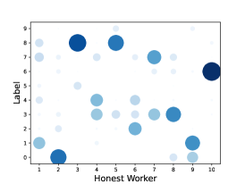
(a) $\alpha=0.1$

(b) $\alpha=0.5$

(c) $\alpha=1$

(d) $\alpha=0.075$

(e) $\alpha=0.2$

Figure 5: Distribution of labels across honest workers on MNIST (row 1) and CIFAR-10 (row 2).

D.2 Algorithm, Distributed System, ML Models, and Hyperparameters

We perform our experiments using Robust-DSGD (see Algorithm 3), which is known to be an order-optimal robust variant of Robust-DGD [3]. On MNIST and Fashion-MNIST, we execute Robust-DSGD in a distributed system composed of $n-f=10$ honest workers, and $f\in\{1,2,3,4,5,7,9\}$ adversarial workers. Furthermore, we train a convolutional neural network (CNN) of 431,080 parameters with batch size $b=25$, $T=1000$, $\gamma=0.1$, and momentum parameter $\beta=0.9$. Moreover, the negative log likelihood (NLL) loss function is used, along with an $\ell_{2}$-regularization of $10^{-4}$. On CIFAR-10, we execute Robust-DSGD using a CNN of 1,310,922 parameters, in a distributed system comprising $n-f=16$ honest workers and $f=1$ adversarial worker. We set $b=50$, $T=2000$, $\beta=0.9$, and $\gamma=0.05$ decaying once at step 1500. Finally, we use the NLL loss function with an $\ell_{2}$ regularization of $10^{-2}$.

Algorithm 3 Robust Stochastic Distributed Gradient Descent (Robust-DSGD)

  Input: Server chooses an initial model ${{\theta}_{1}}\in\mathbb{R}^{d}$, learning rate $\gamma\in\mathbb{R}^{+}$, robust aggregation $\mathbf{F}:\mathbb{R}^{n\times d}\to\mathbb{R}^{d}$, momentum parameter $\beta\in\mathbb{R}^{+}$. Each honest worker ${{w}_{i}}$ sets an initial momentum $m_{0}^{(i)}=0\in\mathbb{R}^{d}$.

  for $t=1$ to $T$ do

     Server broadcasts ${{\theta}_{t}}$ to all workers.

     for each honest worker ${{w}_{i}}$ in parallel do

        Sample a random data point $z^{(i)}$ uniformly from $\mathcal{D}_{i}$.

        Compute stochastic gradient $g_{t}^{(i)}\coloneqq\nabla{\ell(\theta_{t},z^{(i)})}$.

        Update momentum: $m_{t}^{(i)}\coloneqq(1-\beta)g_{t}^{(i)}+\beta m_{t-1}^{(i)}$.

        Send $m_{t}^{(i)}$ to Server.

         // An adversarial worker ${{w}_{j}}$ can send an arbitrary vector in $\mathbb{R}^{d}$ for $m_{t}^{(j)}$

     end for

     Server computes $R_{t}\coloneqq\mathbf{F}\left(m_{t}^{(1)},\dots,\,m_{t}^{(n)}\right)$.

     Server updates the model: ${{\theta}_{t+1}}\coloneqq{{\theta}_{t}}-\gamma\,R_{t}$ .

  end for

  Output: Server outputs $\hat{{{\theta}}}$ chosen uniformly at random from $\{{{\theta}_{1}},\ldots,\,{{\theta}_{T}}\}$.

In order to present the architectures of the ML models used in our experiments, we adopt the following compact terminology introduced in [3].

L(#outputs) represents a fully-connected linear layer, R stands for ReLU activation, S stands for log-softmax, C(#channels) represents a fully-connected 2D-convolutional layer (kernel size 5, padding 0, stride 1), M stands for 2D-maxpool (kernel size 2), B stands for batch-normalization, and D represents dropout (with fixed probability 0.25).

The comprehensive experimental setup, as well as the architecture of the models, are presented in Table 2.

Dataset	(Fashion-)MNIST	CIFAR-10
Data heterogeneity	$\alpha\in\{0.1,0.5,1\}$ and extreme	$\alpha\in\{0.05,0.075,0.1,0.2,0.5\}$
Model type	CNN	CNN
Model architecture	C(20)-R-M-C(20)-R-M-L(500)-R-L(10)-S	(3,32×32)-C(64)-R-B-C(64)-R-B-M-D-C(128)-R-B-C(128)-R-B-M-D-L(128)-R-D-L(10)-S
Number of parameters	431,080	1,310,922
Loss	NLL	NLL
$\ell_{2}$-regularization	$10^{-4}$	$10^{-2}$
Number of steps	$T=1000$	$T=2000$
Learning rate	$\gamma=0.1$	$$\gamma_{t}=\begin{cases}0.05&t\leq 1500\\ 0.00082&1500<t\leq 2000\end{cases}$$
Momentum parameter	$\beta=0.9$	$\beta=0.9$
Batch size	$b=25$	$b=50$
Honest workers	$n-f=10$	$n-f=16$
Adversarial workers	$f\in\{1,2,3,4,5,7,9\}$	$f=1$

Table 2: Experimental setup on (Fashion-)MNIST and CIFAR-10

D.3 Byzantine Attacks

In our experiments, the adversarial workers execute five state-of-the-art adversarial attacks from the Byzantine ML literature, namely sign-flipping (SF) [2], label-flipping (LF) [2], mimic [27], fall of empires (FOE) [43], and a little is enough (ALIE) [6].

The exact functionality of the attacks is detailed below. In every step $t$, let $\overline{m}_{t}$ be an estimation of the true honest momentum at step $t$. In our experiments, we estimate $\overline{m}_{t}$ by averaging the momentums sent by the honest workers in step $t$ of Robust-DSHB. In other words, $\overline{m}_{t}=\frac{1}{|\mathcal{H}|}\sum\limits_{i\in\mathcal{H}}m_{t}^{(i)}$, where $m_{t}^{(i)}$ is the momentum computed by honest worker $w_{i}$ in step $t$.

• SF: the adversarial workers send the vector $-\overline{m}_{t}$ to the server.

• LF: the adversarial workers compute their gradients on flipped labels, and send the flipped gradients to the server. Since the original labels $l$ for (Fashion-)MNIST and CIFAR-10 are in $\{0,...,9\}$, the adversarial workers execute a label flip/rotation by computing their gradients on the modified labels $l^{\prime}=9-l$.

• Mimic: the adversarial workers mimic a certain honest worker by sending its gradient to the server. In order to determine the optimal honest worker for the adversarial workers to mimic, we use the heuristic in [27].

• FOE: the adversarial workers send $(1-\tau)\overline{m}_{t}$ in step $t$ to the server, where $\tau\geq 0$ is a fixed real number representing the attack factor. When $\tau=2$, this attack is equivalent to SF.

• ALIE: the adversarial workers send $\overline{m}_{t}+\tau\sigma_{t}$ in step $t$ to the server, where $\tau\geq 0$ is a fixed real number representing the attack factor, and $\sigma_{t}$ is the coordinate-wise standard deviation of $\overline{m}_{t}$.

Since the FOE and ALIE attacks have $\tau$ as parameter, we implement in our experiments enhanced and adaptive versions of these attacks, where the attack factor is not constant and may be different in every iteration. In every step $t$, we determine the optimal attack factor $\tau_{t}$ through a grid search over a predefined range of values. More specifically, in every step $t$, $\tau_{t}$ takes the value that maximizes the damage inflicted by the adversarial workers, i.e., that maximizes the $l^{2}$ norm of the difference between the average of the honest momentums $\overline{m}_{t}$ and the output of the aggregation $R_{t}$ at the server.

D.4 Benchmarking and Reproducibility

We evaluate the performance of ARC compared to no clipping within the context of Robust-DSGD. Accordingly, we choose $\mathbf{F}\circ$ NNM as aggregator in Algorithm 1, where $\mathbf{F}\in\{$CWTM, GM, CWMed, MK$\}$ is an aggregation rule proved to be $(f,\kappa)$-robust [3]. Composing these aggregation rules with NNM provides them with optimal $(f,\kappa)$-robustness [3]. As benchmark, we also execute the standard DSGD algorithm in the same setting, but in the absence of adversarial workers (i.e., without attack and $f=0$). We plot in Table 1 and Figures 1 and 3 the metric of worst-case maximal accuracy. In other words, for each of the aforementioned five Byzantine attacks, we record the maximal accuracy achieved by Robust-DSGD during the learning under that attack. The worst-case maximal accuracy is thus the smallest maximal accuracy encountered across the five attacks. As the attack executed by adversarial workers cannot be known in advance in a practical system, this metric is critical to accurately evaluate the robustness of aggregation methods, as it gives us an estimate of the potential worst-case performance of the algorithm. Finally, all our experiments are run with seeds 1 to 5 for reproducibility purposes. We provide standard deviation measurements for all our results (across the five seeds). In Appendix E, we show the performance of our algorithm (compared to no clipping) in worst-case maximal accuracy, when varying the heterogeneity level or the number of adversarial workers $f$. We also show some plots showing the evolution of the learning with time under specific attacks (e.g., Figures 8, 9,  10, and 14 in Appendix E), but the totality of these plots can be found in the supplementary material (attached in a folder per dataset).

Appendix E Additional Experimental Results

In this section, we complete the experimental results that could not be placed in the main paper.

E.1 MNIST

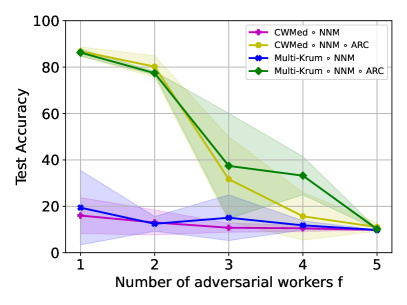
(a) extreme

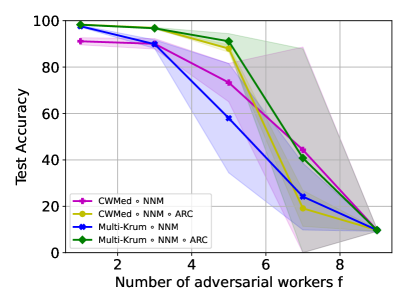
(b) $\alpha=0.5$

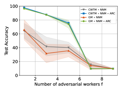
(c) $\alpha=0.1$

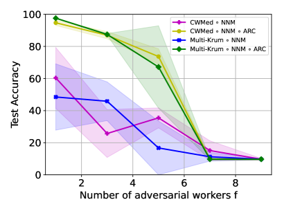
(d) $\alpha=0.1$

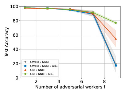
(e) $\alpha=1$

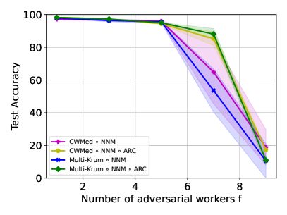
(f) $\alpha=1$

Figure 6: Worst-case maximal accuracies achieved by Robust-DSGD when using ARC compared to no clipping, on heterogeneously-distributed MNIST with $10$ honest workers. We fix the heterogeneity level, and vary the the number of Byzantine workers $f$.

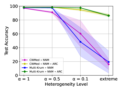
(a) $f=1$

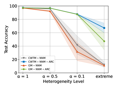
(b) $f=3$

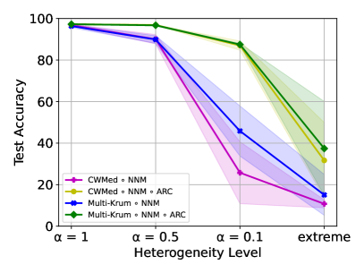
(c) $f=3$

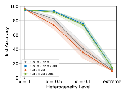
(d) $f=5$

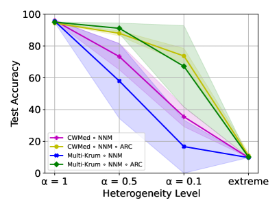
(e) $f=5$

Figure 7: Worst-case maximal accuracies achieved by Robust-DSGD when using ARC compared to no clipping, on heterogeneously-distributed MNIST with $10$ honest workers. We fix the number of Byzantine workers $f$, and vary the heterogeneity level.

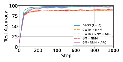
(a) ALIE

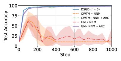
(b) SF

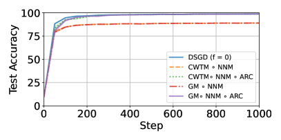
(c) LF

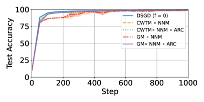
(d) Mimic

Figure 8: Performance of Robust-DSGD when using ARC compared to no clipping, on heterogeneously-distributed MNIST (extreme heterogeneity) with $10$ honest workers and $f=1$, under several attacks. This complements Figure 2c of the main paper.

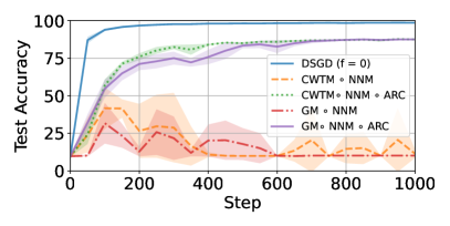
(a) FOE

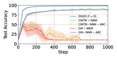
(b) SF

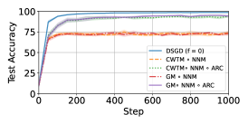
(c) ALIE

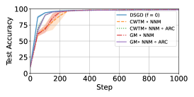
(d) LF

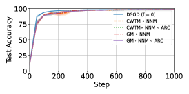
(e) Mimic

Figure 9: Performance of Robust-DSGD when using ARC compared to no clipping, on heterogeneously-distributed MNIST ($\alpha=0.1$) with $10$ honest workers and $f=3$, under several attacks.

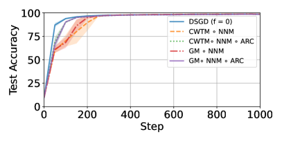
(a) $f=3$

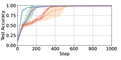
(b) $f=4$

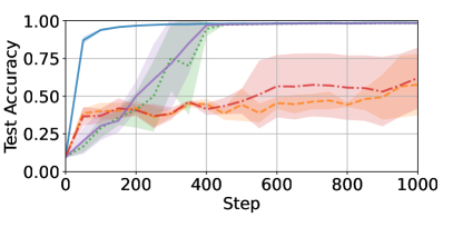
(c) $f=5$

Figure 10: Performance of Robust-DSGD under the LF attack when using ARC compared to no clipping, on heterogeneously-distributed MNIST ($\alpha=0.1$) with $10$ honest workers and varying number of adversarial workers $f$.

E.2 Fashion-MNIST

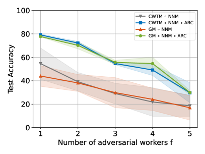
(a) $\alpha=0.1$

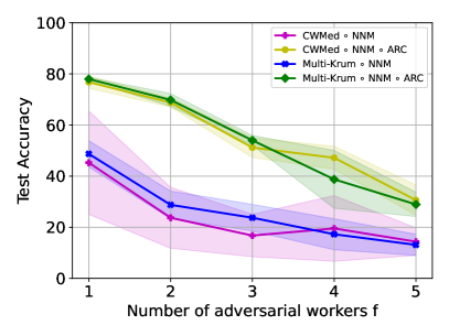
(b) $\alpha=0.1$

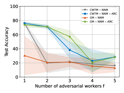
(c) $\alpha=0.05$

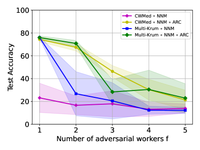
(d) $\alpha=0.05$

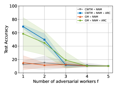
(e) extreme

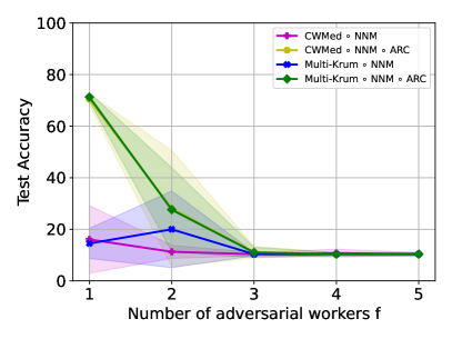
(f) extreme

Figure 11: Worst-case maximal accuracies achieved by Robust-DSGD when using ARC compared to no clipping, on heterogeneously-distributed Fashion-MNIST with $10$ honest workers. We fix the heterogeneity level and vary the number of adversarial workers $f$.

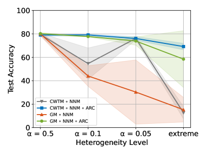
(a) $f=1$

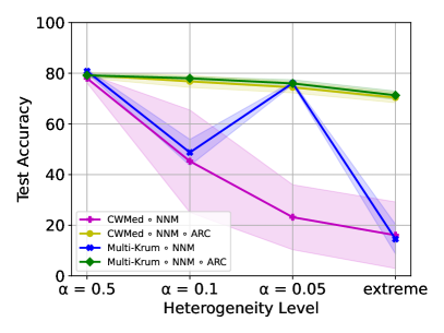
(b) $f=1$

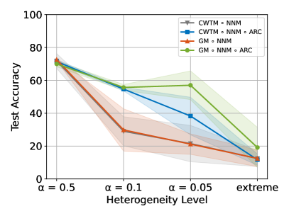
(c) $f=3$

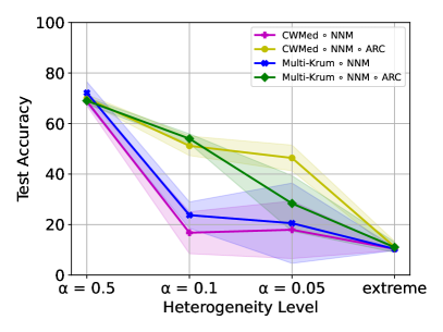
(d) $f=3$

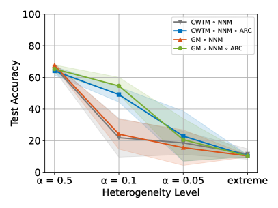
(e) $f=4$

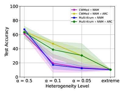
(f) $f=4$

Figure 12: Worst-case maximal accuracies achieved by Robust-DSGD when using ARC compared to no clipping, on heterogeneously-distributed Fashion-MNIST with $10$ honest workers. We fix the number of adversarial workers $f$ and vary the heterogeneity level.

E.3 CIFAR-10

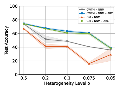
(a) $f=1$

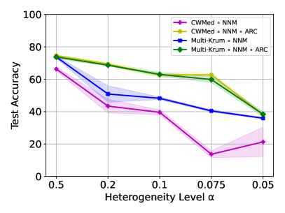
(b) $f=1$

Figure 13: Worst-case maximal accuracies achieved by Robust-DSGD when using ARC compared to no clipping, on heterogeneously-distributed CIFAR-10 with $16$ honest workers. We fix the number of adversarial workers $f=1$ and vary the heterogeneity level.

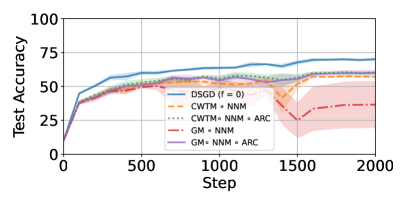
(a) ALIE with CWTM and GM

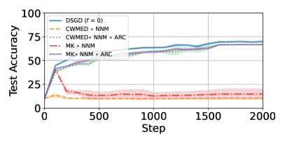
(b) FOE with CWMED and MK

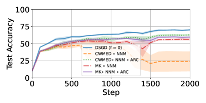
(c) ALIE with CWMED and CWMED

Figure 14: Worst-case maximal accuracies achieved by Robust-DSGD when using ARC compared to no clipping, on heterogeneously-distributed CIFAR-10 ($\alpha=0.075$) with $16$ honest workers and $f=1$ executing ALIE and FOE. This figure complements Figure 4 in the main paper.

Appendix F Static Clipping vs ARC

In this section, we present empirical results on static clipping when used as a pre-aggregation technique in Robust-DSGD, and compare its performance to our proposed adaptive algorithm ARC.

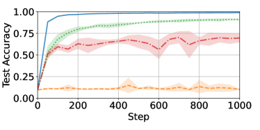
(a) Sign-flipping (SF) [2]

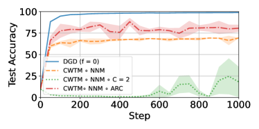
(b) Label-flipping (LF) [2]

Figure 15: Impact of pre-aggregation clipping, specifically static clipping with $C=2$ and ARC, on robust-DGD with aggregation scheme $\mathbf{CWTM}\circ\mathbf{NNM}$, under 2 adversarial attacks: (a) SF and (b) LF. We set $n=13$, $f=3$, and consider the MNIST [11] dataset distributed amongst $n-f=10$ honest workers with extreme heterogeneity.

F.1 Limitations of Static Clipping

We perform our experiments using Robust-DSGD (see Algorithm 3) on (Fashion-)MNIST and CIFAR-10. We consider three different levels of heterogeneity, that we call moderate (corresponding to sampling from a Dirichlet distribution of parameter $\alpha=1$), high ($\alpha=0,1$), and extreme (as explained in Appendix D). On MNIST and Fashion-MNIST, we execute Robust-DSGD in a distributed system composed of $n=15$ workers, among which $f\in\{3,4\}$ are Byzantine. Furthermore, we train a convolutional neural network of 431,080 parameters with batch size $b=25$, $T=1000$, $\gamma=0.1$, and momentum parameter $\beta=0.9$. Moreover, the negative log likelihood loss function is used, along with an $\ell_{2}$-regularization of $10^{-4}$. On CIFAR-10, we execute Robust-DSGD on ResNet-18 [21], in a distributed system comprising $n=9$ workers among which $f\in\{1,2\}$ are Byzantine. We set $b=128$, $T=2000$, $\beta=0.9$, and $\gamma=0.1$ decaying once by 10$\times$ at step 1500. Finally, we use the cross-entropy loss function with an $\ell_{2}$ regularization of $5\times 10^{-4}$.

In our experiments, we examine a wide range of static clipping parameters. Specifically, we choose $C\in\{0.02,0.2,2,20\}$ on MNIST.

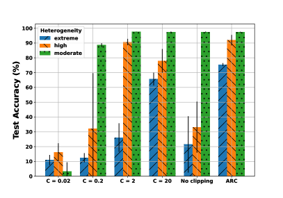
(a) $f=3$

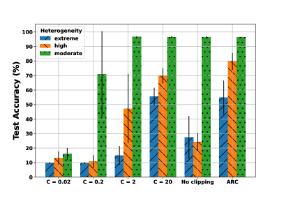
(b) $f=4$

Figure 16: Impact of the clipping strategy and heterogeneity level on the worst-case maximal accuracy achieved by Robust-DSGD against five Byzantine attacks on heterogeneous MNIST with $n=15$ workers. CWTM $\circ$ NNM is used as aggregation. DSGD reaches at least 98.5% in accuracy in all heterogeneity regimes.

Unreliability due to the attack. First, the efficacy of static clipping is significantly influenced by the type of Byzantine attack executed during the learning process. To illustrate, while $C=2$ exhibits the best performance under the SF attack [2], depicted in Figure 15, it leads to a complete collapse of learning under LF [2]. Consequently, identifying a static clipping threshold $C$ that consistently performs well in practice against any attack is difficult (if not impossible). This highlights the fragility of static clipping, as the unpredictable nature of the Byzantine attack, a parameter that cannot be a priori known, can significantly degrade the performance of the chosen static clipping approach.

Unreliability due to the heterogeneity model. Second, the robustness under static clipping is notably influenced by the level of heterogeneity present across the datasets of honest workers. To illustrate this impact, we present in Figure 16 the performances of Robust-DSGD for different levels of heterogeneity (moderate, high, and extreme) and different values of $C$. In the left plot of Figure 16, $C=2$ emerges as the best static clipping threshold when the heterogeneity is high whereas $C=20$ appears to be sub-optimal. On the other hand, under extreme heterogeneity, the accuracy associated to $C=2$ diminishes drastically while $C=20$ becomes a better choice. Intuitively, in heterogeneous scenarios, honest gradients become large in $l^{2}$-norm, due to the increasingly detrimental effect of Byzantine attacks. Consequently, we must increase the static clipping threshold. Failing to do so could introduce a significant bias. More details on this observation can be found in Figure 17. This highlights the intricate dependence of the performance of static clipping on data heterogeneity, and emphasizes the necessity to fine-tune static clipping strategies prior to the learning.

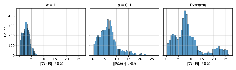
Figure 17: Distribution of the norms of honest gradients during the learning on heterogeneous MNIST. There are $f=3$ Byzantine workers (among $n=15$) executing the LF attack. CWTM $\circ$ NNM is used as aggregation method.

Unreliability due to the number of Byzantine workers. Last but not least, the number of Byzantine workers $f$ also affects the efficacy of static clipping. As seen in Figure 16, $C=2$ leads to the highest accuracy among static clipping strategies when $f=3$ in high heterogeneity, but cannot be used when $f=4$ as its corresponding accuracy drops below 50% (see right plot of Figure 16).

Overall, our empirical findings reveal that there is no single value of $C$ for which static clipping consistently delivers satisfactory performance across the various settings. We have also shown that the performance of static clipping is greatly influenced on typically uncontrollable parameters, such as data heterogeneity and the nature of the Byzantine attack. Indeed, it should be noted that explicitly estimating these parameters is challenging (if not impossible) in a distributed setting. First, since the server does not have direct access to the data, it cannot estimate the degree of heterogeneity. Second, as (by definition) a Byzantine worker can behave in an unpredictable manner, we cannot adjust $C$ to the attack(s) being executed by the Byzantine workers. This highlights the necessity for a robust clipping alternative that can naturally adapt to the setting in which it is deployed.

F.2 Empirical Benefits of ARC

In contrast to static clipping, ARC is adaptive, delivering consistent performance across diverse levels of heterogeneity, Byzantine attacks, and number of Byzantine workers.

Adaptiveness.

ARC dynamically adjusts its clipping parameter $C_{t}$ based on the norms of honest momentums at step $t$, avoiding static over-clipping or under-clipping. This adaptability is evident in Figure 18, where $C_{t}$ consistently decreases with time under all attacks, an expected behavior when reaching convergence. Moreover, Figure 18 also illustrates that any surge in the norm of the honest mean corresponds to a direct increase in $C_{t}$, highlighting the adaptive nature of ARC.

Robust performance across heterogeneity regimes.

The efficacy of our solution is illustrated in Figure 16, showcasing a consistently robust performance for all considered heterogeneity levels. Specifically, in scenarios of moderate heterogeneity where clipping may not be essential, ARC matches the performance of No clipping as well as static strategies $C=2$ and $C=20$. Conversely, the left plot of Figure 16 shows that under high and extreme heterogeneity, ARC surpasses the best static clipping strategy in terms of accuracy, highlighting the effectiveness of our approach.

Robust performance across Byzantine regimes.

ARC exhibits robust performance across diverse Byzantine scenarios, encompassing variations in both the type of Byzantine attack and the number of Byzantine workers $f$. As depicted in Figures 15 and 16, ARC consistently yields robust performance, regardless of the Byzantine attack. In extreme heterogeneity with $f=3$, ARC maintains an accuracy of 75%, while $C=2$ demonstrates a subpar worst-case accuracy of 25% (also refer to the right plot of Figure 15). Furthermore, despite the increase in the number of Byzantine workers to $f=4$, ARC remains the top-performing clipping approach among all considered strategies.

This analysis underscores the empirical superiority of ARC over static clipping methods, eliminating the reliance on data heterogeneity and the specific Byzantine regime. Similar trends are also observed in Figure 19, when executing Robust-DSGD using other aggregation methods such as CWMed $\circ$ NNM, GM $\circ$ NNM, and Multi-Krum $\circ$ NNM.

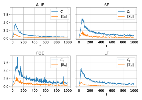
Figure 18: Evolution of the adaptive clipping parameter $C_{t}$ of ARC compared to the norm of the honest mean during the learning on heterogeneous MNIST ($\alpha=1$). There are $f=3$ Byzantine workers among $n=15$. CWTM $\circ$ NNM is used as aggregation. ARC dynamically adjusts its clipping parameter $C_{t}$ based on the norms of honest momentums at step $t$, avoiding static over-clipping or under-clipping. This adaptability is evident in under all attacks, where $C_{t}$ consistently decreases with time, an expected behavior when reaching convergence.

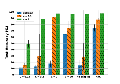
(a) CWMed $\circ$ NNM

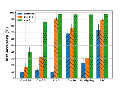
(b) GM $\circ$ NNM

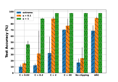
(c) MK $\circ$ NNM

Figure 19: Impact of the clipping strategy on the worst-case maximal accuracy achieved during the learning against five Byzantine attacks on heterogeneous MNIST, with $f=3$ and $n=15$.

References

• [1] M. Abadi, A. Chu, I. Goodfellow, H. B. McMahan, I. Mironov, K. Talwar, and L. Zhang. Deep learning with differential privacy. In Proceedings of the 2016 ACM SIGSAC conference on computer and communications security, pages 308–318, 2016.
• [2] Z. Allen-Zhu, F. Ebrahimianghazani, J. Li, and D. Alistarh. Byzantine-resilient non-convex stochastic gradient descent. In International Conference on Learning Representations, 2020.
• [3] Y. Allouah, S. Farhadkhani, R. Guerraoui, N. Gupta, R. Pinot, and J. Stephan. Fixing by mixing: A recipe for optimal byzantine ml under heterogeneity. In F. Ruiz, J. Dy, and J.-W. van de Meent, editors, Proceedings of The 26th International Conference on Artificial Intelligence and Statistics, volume 206 of Proceedings of Machine Learning Research, pages 1232–1300. PMLR, 25–27 Apr 2023.
• [4] Y. Allouah, R. Guerraoui, N. Gupta, R. Pinot, and G. Rizk. Robust distributed learning: Tight error bounds and breakdown point under data heterogeneity. In Thirty-seventh Conference on Neural Information Processing Systems, 2023.
• [5] Y. Allouah, R. Guerraoui, N. Gupta, R. Pinot, and J. Stephan. On the privacy-robustness-utility trilemma in distributed learning. In International Conference on Machine Learning, number 202, 2023.
• [6] G. Baruch, M. Baruch, and Y. Goldberg. A little is enough: Circumventing defenses for distributed learning. In H. Wallach, H. Larochelle, A. Beygelzimer, F. d'Alché-Buc, E. Fox, and R. Garnett, editors, Advances in Neural Information Processing Systems, volume 32. Curran Associates, Inc., 2019.
• [7] P. Blanchard, E. M. El Mhamdi, R. Guerraoui, and J. Stainer. Machine learning with adversaries: Byzantine tolerant gradient descent. In I. Guyon, U. V. Luxburg, S. Bengio, H. Wallach, R. Fergus, S. Vishwanathan, and R. Garnett, editors, Advances in Neural Information Processing Systems 30, pages 119–129. Curran Associates, Inc., 2017.
• [8] L. Bottou, F. E. Curtis, and J. Nocedal. Optimization methods for large-scale machine learning. Siam Review, 60(2):223–311, 2018.
• [9] S. Boyd and L. Vandenberghe. Convex optimization. Cambridge university press, 2004.
• [10] Y. Chen, L. Su, and J. Xu. Distributed statistical machine learning in adversarial settings: Byzantine gradient descent. Proceedings of the ACM on Measurement and Analysis of Computing Systems, 1(2):1–25, 2017.
• [11] L. Deng. The mnist database of handwritten digit images for machine learning research. IEEE Signal Processing Magazine, 29(6):141–142, 2012.
• [12] E. M. El Mhamdi, R. Guerraoui, and S. Rouault. The hidden vulnerability of distributed learning in Byzantium. In J. Dy and A. Krause, editors, Proceedings of the 35th International Conference on Machine Learning, volume 80 of Proceedings of Machine Learning Research, pages 3521–3530. PMLR, 10–15 Jul 2018.
• [13] S. Farhadkhani, R. Guerraoui, N. Gupta, L.-N. Hoang, R. Pinot, and J. Stephan. Robust collaborative learning with linear gradient overhead. In A. Krause, E. Brunskill, K. Cho, B. Engelhardt, S. Sabato, and J. Scarlett, editors, Proceedings of the 40th International Conference on Machine Learning, volume 202 of Proceedings of Machine Learning Research, pages 9761–9813. PMLR, 23–29 Jul 2023.
• [14] S. Farhadkhani, R. Guerraoui, N. Gupta, R. Pinot, and J. Stephan. Byzantine machine learning made easy by resilient averaging of momentums. In K. Chaudhuri, S. Jegelka, L. Song, C. Szepesvari, G. Niu, and S. Sabato, editors, Proceedings of the 39th International Conference on Machine Learning, volume 162 of Proceedings of Machine Learning Research, pages 6246–6283. PMLR, 17–23 Jul 2022.
• [15] X. Glorot and Y. Bengio. Understanding the difficulty of training deep feedforward neural networks. In Proceedings of the thirteenth international conference on artificial intelligence and statistics, pages 249–256. JMLR Workshop and Conference Proceedings, 2010.
• [16] I. Goodfellow, Y. Bengio, and A. Courville. Deep Learning. MIT Press, 2016. http://www.deeplearningbook.org.
• [17] E. Gorbunov, S. Horváth, P. Richtárik, and G. Gidel. Variance reduction is an antidote to byzantines: Better rates, weaker assumptions and communication compression as a cherry on the top. In The Eleventh International Conference on Learning Representations, 2023.
• [18] R. Guerraoui, N. Gupta, and R. Pinot. Byzantine machine learning: A primer. ACM Computing Surveys, 2023.
• [19] R. Guerraoui, N. Gupta, R. Pinot, S. Rouault, and J. Stephan. Differential privacy and byzantine resilience in sgd: Do they add up? In Proceedings of the 2021 ACM Symposium on Principles of Distributed Computing, PODC’21, page 391–401, New York, NY, USA, 2021. Association for Computing Machinery.
• [20] N. Gupta and N. H. Vaidya. Fault-tolerance in distributed optimization: The case of redundancy. In Proceedings of the 39th Symposium on Principles of Distributed Computing, pages 365–374, 2020.
• [21] K. He, X. Zhang, S. Ren, and J. Sun. Deep residual learning for image recognition, 2015.
• [22] C. A. R. Hoare. Algorithm 65: Find. Commun. ACM, 4(7):321–322, jul 1961.
• [23] T.-M. H. Hsu, H. Qi, and M. Brown. Measuring the effects of non-identical data distribution for federated visual classification, 2019.
• [24] T.-M. H. Hsu, H. Qi, and M. Brown. Measuring the effects of non-identical data distribution for federated visual classification, 2019.
• [25] P. Kairouz, H. B. McMahan, B. Avent, A. Bellet, M. Bennis, A. N. Bhagoji, K. Bonawitz, Z. Charles, G. Cormode, R. Cummings, R. G. L. D’Oliveira, H. Eichner, S. E. Rouayheb, D. Evans, J. Gardner, Z. Garrett, A. Gascón, B. Ghazi, P. B. Gibbons, M. Gruteser, Z. Harchaoui, C. He, L. He, Z. Huo, B. Hutchinson, J. Hsu, M. Jaggi, T. Javidi, G. Joshi, M. Khodak, J. Konecný, A. Korolova, F. Koushanfar, S. Koyejo, T. Lepoint, Y. Liu, P. Mittal, M. Mohri, R. Nock, A. Özgür, R. Pagh, H. Qi, D. Ramage, R. Raskar, M. Raykova, D. Song, W. Song, S. U. Stich, Z. Sun, A. T. Suresh, F. Tramèr, P. Vepakomma, J. Wang, L. Xiong, Z. Xu, Q. Yang, F. X. Yu, H. Yu, and S. Zhao. Advances and open problems in federated learning. Foundations and Trends® in Machine Learning, 14(1–2):1–210, 2021.
• [26] S. P. Karimireddy, L. He, and M. Jaggi. Learning from history for Byzantine robust optimization. International Conference On Machine Learning, Vol 139, 139, 2021.
• [27] S. P. Karimireddy, L. He, and M. Jaggi. Byzantine-robust learning on heterogeneous datasets via bucketing. In International Conference on Learning Representations, 2022.
• [28] S. P. Karimireddy, S. Kale, M. Mohri, S. Reddi, S. Stich, and A. T. Suresh. Scaffold: Stochastic controlled averaging for federated learning. In International Conference on Machine Learning, pages 5132–5143. PMLR, 2020.
• [29] S. Khirirat, E. Gorbunov, S. Horváth, R. Islamov, F. Karray, and P. Richtárik. Clip21: Error feedback for gradient clipping. arXiv preprint arXiv:2305.18929, 2023.
• [30] A. Koloskova, H. Hendrikx, and S. U. Stich. Revisiting gradient clipping: stochastic bias and tight convergence guarantees. In Proceedings of the 40th International Conference on Machine Learning, ICML’23. JMLR.org, 2023.
• [31] A. Krizhevsky, V. Nair, and G. Hinton. The CIFAR-10 dataset. online: http://www. cs. toronto. edu/kriz/cifar. html, 55(5), 2014.
• [32] L. Lamport, R. Shostak, and M. Pease. The Byzantine generals problem. ACM Trans. Program. Lang. Syst., 4(3):382–401, jul 1982.
• [33] S. Liu, N. Gupta, and N. H. Vaidya. Approximate Byzantine fault-tolerance in distributed optimization. In Proceedings of the 2021 ACM Symposium on Principles of Distributed Computing, PODC’21, page 379–389, New York, NY, USA, 2021. Association for Computing Machinery.
• [34] G. Long, Y. Tan, J. Jiang, and C. Zhang. Federated learning for open banking. In Federated Learning: Privacy and Incentive, pages 240–254. Springer, 2020.
• [35] G. Malinovsky, P. Richtárik, S. Horváth, and E. Gorbunov. Byzantine robustness and partial participation can be achieved simultaneously: Just clip gradient differences. arXiv preprint arXiv:2311.14127, 2023.
• [36] B. McMahan, E. Moore, D. Ramage, S. Hampson, and B. A. y. Arcas. Communication-Efficient Learning of Deep Networks from Decentralized Data. In A. Singh and J. Zhu, editors, Proceedings of the 20th International Conference on Artificial Intelligence and Statistics, volume 54 of Proceedings of Machine Learning Research, pages 1273–1282. PMLR, 20–22 Apr 2017.
• [37] E. M. E. Mhamdi, R. Guerraoui, and S. Rouault. Distributed momentum for byzantine-resilient stochastic gradient descent. In International Conference on Learning Representations, 2021.
• [38] D. C. Nguyen, Q.-V. Pham, P. N. Pathirana, M. Ding, A. Seneviratne, Z. Lin, O. Dobre, and W.-J. Hwang. Federated learning for smart healthcare: A survey. ACM Comput. Surv., 55(3), feb 2022.
• [39] V. Pichapati, A. T. Suresh, F. X. Yu, S. J. Reddi, and S. Kumar. Adaclip: Adaptive clipping for private SGD. CoRR, abs/1908.07643, 2019.
• [40] L. Su and N. H. Vaidya. Fault-tolerant multi-agent optimization: optimal iterative distributed algorithms. In Proceedings of the 2016 ACM symposium on principles of distributed computing, pages 425–434, 2016.
• [41] S. Vaswani, F. Bach, and M. Schmidt. Fast and faster convergence of SGD for over-parameterized models and an accelerated perceptron. In The 22nd international conference on artificial intelligence and statistics, pages 1195–1204. PMLR, 2019.
• [42] H. Xiao, K. Rasul, and R. Vollgraf. Fashion-mnist: a novel image dataset for benchmarking machine learning algorithms. arXiv preprint arXiv:1708.07747, 2017.
• [43] C. Xie, O. Koyejo, and I. Gupta. Fall of empires: Breaking byzantine-tolerant sgd by inner product manipulation. In R. P. Adams and V. Gogate, editors, Proceedings of The 35th Uncertainty in Artificial Intelligence Conference, volume 115 of Proceedings of Machine Learning Research, pages 261–270. PMLR, 22–25 Jul 2020.
• [44] D. Yin, Y. Chen, R. Kannan, and P. Bartlett. Byzantine-robust distributed learning: Towards optimal statistical rates. In International Conference on Machine Learning, pages 5650–5659. PMLR, 2018.
• [45] B. Zhang, J. Jin, C. Fang, and L. Wang. Improved analysis of clipping algorithms for non-convex optimization. In Proceedings of the 34th International Conference on Neural Information Processing Systems, NIPS’20, Red Hook, NY, USA, 2020. Curran Associates Inc.
• [46] J. Zhang, T. He, S. Sra, and A. Jadbabaie. Why gradient clipping accelerates training: A theoretical justification for adaptivity. In International Conference on Learning Representations, 2020.
• [47] X. Zhang, X. Chen, M. Hong, S. Wu, and J. Yi. Understanding clipping for federated learning: Convergence and client-level differential privacy. In International Conference on Machine Learning, pages 26048–26067. PMLR, 2022.
• [48] H. Zhu and Q. Ling. Bridging differential privacy and Byzantine-robustness via model aggregation. In L. D. Raedt, editor, Proceedings of the Thirty-First International Joint Conference on Artificial Intelligence, IJCAI-22, pages 2427–2433. International Joint Conferences on Artificial Intelligence Organization, 7 2022. Main Track.