A hybrid systems framework for data-based adaptive control of linear time-varying systems

Abstract

We consider the data-driven stabilization of discrete-time linear time-varying systems. The controller is defined as a linear state-feedback law whose gain is adapted to the plant changes through a data-based event-triggering rule. To do so, we monitor the evolution of a data-based Lyapunov function along the solution. When this Lyapunov function does not satisfy a designed desirable condition, an episode is triggered to update the controller gain and the corresponding Lyapunov function using the last collected data. The resulting closed-loop dynamics hence exhibits both physical jumps, due to the system dynamics, and episodic jumps, which naturally leads to a hybrid discrete-time system. We leverage the inherent robustness of the controller and provide general conditions under which various stability notions can be established for the system. Two notable cases where these conditions are satisfied are treated, and numerical results illustrating the relevance of the approach are discussed.

Data-driven control; hybrid systems; Lyapunov stability; event-triggered control; adaptive control; time-varying systems

1 Introduction

The problem of designing controllers for dynamical systems only using data trajectories is a very active area of research. Motivations include the increasing complexity of modern engineering and cyberphysical applications, the large availability of data and the time and cost savings potentially achieved by avoiding the modeling or system identification phase. Additionally, for systems changing over time, updating models during operation might not always be possible because by the time sufficiently many data for an accurate identification have been collected, the system dynamics could have substantially changed. In this work, we develop a framework for the synthesis of data-based adaptive controllers for linear time-varying (LTV) systems with unknown state and input matrices, undergoing unpredicted time-variations. This problem poses two conceptual challenges. From a learning perspective, one should answer the questions of how and when to update the controller on the basis of data measured on-line. From a technical perspective, proving closed-loop properties of the nonlinear time-varying interconnection between the plant and such an adaptive controller requires careful modeling and analysis steps. To address these challenges, we propose to cast this problem as an instance of hybrid (discrete-time) dynamical systems [1, Section 4] and blend concepts from the event-triggered control literature e.g., [2] with recent results on data-based control [3]. Before elaborating more on the proposed approach, we briefly review the related literature for linear time-invariant (LTI) and LTV systems.

In the context of unknown LTI systems, the idea of designing a static state-feedback controller such that the closed-loop dynamics enjoys a favourable Lyapunov property can be traced back to [3]. Here, stabilizing controllers are obtained by solving linear matrix inequalities (LMI) formulated in terms of suitable data matrices containing state and input trajectories collected offline, that is prior to the controller deployment. Different technical solutions to achieve a similar goal were also proposed in other works addressing the problems of noisy data [4] and integration of prior knowledge in the form of a nominal model [5], to cite a few. Whereas most of the approaches proposed in the literature use offline data and thus the resulting controller is fixed during operation, a few works studied adaptive data-driven controllers, whereby the control law is modified during operation in response to plant’s changes. In [6] the authors extended [3] to the class of switched linear systems by using on-line collected data. The control update is performed at every time instant and the stability guarantees rely on dwell-time conditions. A similar approach was recently used in [7], where the more general class of LTV is considered, and practical stability guarantees are obtained by implementing a periodic update based on the assumed rate of change of the system matrices. Data-driven control of LTV systems is also studied in [8], where no on-line update is performed and finite horizon guarantees are obtained by assuming that the data collected offline describe the behavior of the system during operation. To the best of the authors’ knowledge, there is no prior work that considers stabilizing data-driven adaptive controllers for general LTV systems where on-line data are used not only to update controllers, but also to decide on when the update should be performed.

We thus model the problem as a hybrid discrete-time system in the sense of [1, Section 4], which exhibits two types of jumps that are either due to the system dynamics, or to the triggering of a new episode. By episode, we mean the update of the controller gain, chosen here as a linear state-feedback gain, based on the last collected state and input data. We first present novel results for this class of hybrid dynamical systems, whose applicability goes beyond the scope of this work (Section 3). We then introduce all the variables needed to describe the overall closed-loop model and thus to obtain a hybrid discrete-time model, which allows us to formally state the stability problem (Section 4). The objective is to design both the controller gain update rule as well as the episode-triggering law for the closed-loop system to have suitable stability properties. We also provide an explicit construction of the controller update rule by revisiting the work in [3] adapted to the LTV context (Section 5). Afterwards, we design the episode-triggering rule by exploiting a data-driven Lyapunov function obtained in the controller gain update step (Section 6). The triggering rule consists in monitoring whether this Lyapunov function satisfies a desired decay rate along the solution. When this is not the case, it means that the time-variations undergone by the plant require a new controller to be designed and thus a new episode to be triggered. Similar triggering rules have been proposed in e.g., [9, 10, 11, 12], where the set-up is different as a triggering instant refers there to a sampling instant, and not to a controller and Lyapunov function update, which leads to major modeling, analysis and design differences. In Section 7 we exploit the previous constructive results to establish sufficient conditions under which stability properties hold. A feature of these conditions is their generality, which allows covering a range of scenarios. On the other hand, these conditions may be difficult to check only based on data. We therefore derive more specific conditions relating instances of the variations of the system matrices to the stability guarantees. We finally provide two numerical examples to illustrate the proposed methodology and compare it to time-triggered controller updates strategies like in [7]. The proposed approach show significant performance improvements and less episode triggering.

Compared to the related results mentioned above, the results do not explicitly rely on conditions on the variations of the system matrices like in e.g., [7, 6] and the controller gain updates only occur when needed and not in a prefixed manner. We also highlight that, although recent works have used event-triggered concepts in the context of data-driven control e.g., [13, 14, 12], the set-up here is very different. In these references, the control law is fixed once for all and the triggering rule is used to define the time at which sensor or actuator information is updated. In this work, communication between the plant and the controller occurs at every physical time step and the triggering instant is the mechanism by which the controller gain is adapted over time. These key differences require complete different methodological tools.

2 Notation

$\mathbb{R}$ denotes the set of real numbers, $\mathbb{R}_{\geq 0}:=[0,\infty)$, $\mathbb{R}_{>0}:=(0,\infty)$, $\mathbb{Z}$ the set of integers, $\mathbb{Z}_{\geq p}:=\{p,p+1,\ldots\}$ with $p\in\mathbb{Z}$ and $\emptyset$ the empty set. Given $k_{1},k_{2}\in\mathbb{Z}_{\geq 0}$ with $k_{1}<k_{2}$, we denote by $[k_{1},k_{2}]$ the finite set $\{k_{1},k_{1}+1,..,k_{2}-1,k_{2}\}$. Given $n\in\mathbb{Z}_{\geq 1}$, we denote by $\mathbb{S}^{n}$ the set of real symmetric matrices of dimension $n$ and by $\mathbb{S}^{n}_{\succeq 0}$ and $\mathbb{S}^{n}_{\succ 0}$ the set of real symmetric positive semi-definite and positive definite matrices of dimension $n$, respectively. When $S\in\mathbb{S}_{\succ 0}^{n}$ with $n\in\mathbb{Z}_{\geq 1}$, its minimum and maximum eigenvalues are denoted $\lambda_{\min}(S)$ and $\lambda_{\max}(S)$, respectively. The determinant of a real square matrix is denoted $\text{det}(\cdot)$, and its spectrum norm by $\|\cdot\|$. We use $\left[\begin{smallmatrix}A&B\\ \star&C\end{smallmatrix}\right]$ in place of $\left[\begin{smallmatrix}A&B\\ B^{\top}&C\end{smallmatrix}\right]$ for the sake of convenience. Given square matrices $A_{1},\ldots,A_{n}\in\mathbb{R}^{n\times n}$ with $n\in\mathbb{Z}_{\geq 1}$, we use $\text{diag}(A_{1},\ldots,A_{n})$ to denote the block diagonal matrix of dimension $n^{2}\times n^{2}$ whose block diagonal components are $A_{1},\ldots,A_{n}$. The symbol $\otimes$ stands for the Kronecker product for matrices. Given $n,T\in\mathbb{Z}_{\geq 1}$, $\mathcal{N}_{n,T}$ is the map from $\mathbb{R}^{n\times T}$ to $\mathbb{R}^{nT\times T}$ such that, for any $Z=[z_{1},\ldots,z_{T}]\in\mathbb{R}^{n\times T}$, $\mathcal{N}_{n,T}(Z)=\left[\begin{smallmatrix}z_{0}&0&\ldots&0\\ 0&z_{1}&\ldots&\vdots\\ \vdots&\ddots&\ddots&\vdots\\ 0&\cdots&\cdots&z_{T-1}\end{smallmatrix}\right]$, and we write $\mathcal{N}(Z)$ when $n$ and $T$ are clear from the context. Given $n,p,q\in\mathbb{Z}_{\geq 1}$ with $q\geq 2$ and a matrix $M=(M_{ij})_{(i,j)\in[1,n]\times[1,p]}\in\mathbb{R}^{n\times p}$, $M_{q:p}$ stands for the matrix $(M_{ij})_{(i,j)\in[1,n]\times[q,p]}\in\mathbb{R}^{n\times(p-q+1)}$ that is, matrix $M$ truncated from its first $q-1$ columns. We use $I_{N}$ to denote the identity matrix of size $N\in\mathbb{Z}_{\geq 1}$, and $\mathbf{1}_{N}$ for the unitary vector of $\mathbb{R}^{N}$. The notation $(x,y)$ stands for $[x^{\top},\,y^{\top}]^{\top}$, where $(x,y)\in\mathbb{R}^{n}\times\mathbb{R}^{m}$ and $n,m\in\mathbb{Z}_{\geq 1}$. The symbols $\lor$ and $\land$ stand for the “or” and “and” logic operators, respectively.

When we write $G:\mathcal{S}_{1}\rightrightarrows\mathcal{S}_{2}$ for some sets $\mathcal{S}_{1}$, $\mathcal{S}_{2}$, it means that $G$ is a set-valued map from $\mathcal{S}_{1}$ to $\mathcal{S}_{2}$. We consider $\mathcal{K}$, $\mathcal{K}_{\infty}$ and $\mathcal{KL}$ functions as defined in [15, Section 3.5], and we say that a continuous function from $\mathbb{R}_{\geq 0}\to\mathbb{R}_{\geq 0}$ is of class $\mathcal{L}$ if it is non-increasing and converges to $0$ at infinity. We also write $\beta\in\exp-\mathcal{KL}$ when $\beta:\mathbb{R}_{\geq 0}\times\mathbb{R}_{\geq 0}\to\mathbb{R}_{\geq 0}$ and there exist $c_{1}\geq 1$ and $c_{2}>0$ such that $\beta(s,t)=c_{1}e^{-c_{2}t}s$ for any $(s,t)\in\mathbb{R}_{\geq 0}\times\mathbb{R}_{\geq 0}$. Given a function $\alpha:\mathbb{R}_{\geq 0}\times\mathcal{S}\to\mathbb{R}_{\geq 0}$ with $\mathcal{S}\subset\mathbb{R}^{n}$ for some $n\in\mathbb{Z}_{\geq 1}$, that is invertible in its first argument, we denote the corresponding inverse (with respect to the first argument) as $\alpha^{-1}(\cdot,z)$ for any $z\in\mathcal{S}$. Finally, for a (set-valued) map $f$ and $N\in\mathbb{Z}_{\geq 1}$, $f^{N}$ stands for the $N^{\text{th}}$ composition of $f$ with itself when it is well-defined.

3 Background

3.1 Discrete-time hybrid systems

We consider dynamical systems given by

$$\left\{\begin{array}[]{rlllll}q^{+}=f(q)&&q\in\mathcal{C}\\ q^{+}\in G(q)&&q\in\mathcal{D},\end{array}\right.$$ (1)

where $\mathcal{C}\subset\mathbb{R}^{n_{q}}$, $\mathcal{D}\subset\mathbb{R}^{n_{q}}$, $f:\mathcal{C}\to\mathbb{R}^{n_{q}}$ and $G:\mathcal{D}\rightrightarrows\mathbb{R}^{n_{q}}$ a set-valued map with $n_{q}\in\mathbb{Z}_{\geq 1}$; see [1, Section 4]. Solutions to (1) exhibit two types of jumps depending on whether they belong to set $\mathcal{C}$ or to set $\mathcal{D}$ as formalized below. In the setting of this paper, $q$ is the concatenation of the plant state vector and some auxiliary variables, $\mathcal{C}$ is the region of the state space where the system is operated, and $\mathcal{D}$ is the region of state space where a new controller is learned and, using the terminology adopted in the rest of the work, a new episode is triggered; see Section 4. We therefore parameterize solutions to (1) using two different times as in [1, Section 4] to distinguish jumps that are due to the dynamics on $\mathcal{C}$ and jumps that are due to the dynamics defined on $\mathcal{D}$. This is the reason why we call system (1) a hybrid discrete-time system.

3.2 Solution concept

We adopt the notion of solution advocated in [1, Section 4]. A subset $E\subset\mathbb{Z}_{\geq 0}\times\mathbb{Z}_{\geq 0}$ is a compact discrete time domain if $E=\bigcup_{j=0}^{J-1}\bigcup_{k=k_{j}}^{k_{j+1}}(k,j)$ for some finite sequence $0=k_{0}\leq k_{1}\leq\ldots\leq k_{J}$, $k_{j}\in\mathbb{Z}_{\geq 0}$ for every $j\in[0,J]$ with $J\in\mathbb{Z}_{\geq 1}$, and it is a discrete time domain if for any $(k,j)\in E$, $E\cap([0,k]\times[0,j])$ is a compact discrete time domain [1, Definition 4.1]. A function $q:\text{dom}\,q\to\mathbb{R}^{n_{q}}$ is a discrete arc if $\text{dom}\,q$ is a discrete time domain [1, Definition 4.2]. We are ready to define solutions to (1).

Definition 1 ([1, Definition 4.3])

A discrete arc $q:\text{dom}\,q\to\mathbb{R}^{n_{q}}$ is a solution to system (1) if

1. for all $k,j\in\mathbb{Z}_{\geq 0}$ such that $(k,j),(k+1,j)\in\text{dom}\,q$, $q(k,j)\in\mathcal{C}$ and $q(k+1,j)=f(q(k,j))$,

2. for all $k,j\in\mathbb{Z}_{\geq 0}$ such that $(k,j),(k,j+1)\in\text{dom}\,q$, $q(k,j)\in\mathcal{D}$ and $q(k,j+1)\in G(q(k,j))$. $\Box$

Definition 1 essentially means that a solution to (1) jumps according to: (i) the map $f$ when it lies in $\mathcal{C}$; (ii) the set-valued map $G$ when it lies in $\mathcal{D}$; (iii) either $f$ or $G$ when it lies in $\mathcal{C}\cap\mathcal{D}$. We note that, as mentioned above, solutions to (1) are parameterized by two times: $k$ and $j$, which in our setting respectively correspond to the physical time and the episodic time that is, the number of episodes experienced so far by the solution. We call a pair $(k,j)$ a hybrid time.

We give a few other definitions relevant to our work.

Definition 2

A solution $q$ to (1) is:

• maximal if there does not exist another solution $q^{\prime}$ to (1) such that $\text{dom}\,q$ is a proper subset of $\text{dom}\,q^{\prime}$ and $q(k,j)=q^{\prime}(k,j)$ for any $(k,j)\in\text{dom}\,q$;

• complete if $\text{dom}\,q$ is unbounded;

• $k$-complete if $\sup\{k\in\mathbb{Z}_{\geq 0}\,:\,\exists j\in\mathbb{Z}_{\geq 0}\,\,(k,j)\in\text{dom}\,q\}=\infty$. $\Box$

We provide below conditions for any maximal solution to (1) to be ($k$-)complete.

Proposition 1

Consider system (1), the following holds.

1. Any maximal solution is complete if and only if $f(\mathcal{C})\cup G(\mathcal{D})\subset\mathcal{C}\cup\mathcal{D}$.

2. Any maximal solution is $k$-complete if $f(\mathcal{C})\cup G(\mathcal{D})\subset\mathcal{C}\cup\mathcal{D}$ and there exists $N\in\mathbb{Z}_{\geq 1}$ such that $G^{N}(\mathcal{D})\cap\mathcal{D}=\emptyset$. $\Box$

Proof: (i) Suppose that any maximal solution to (1) is complete. This implies that for any point $q$ in $\mathcal{C}$, $f(q)$ belongs to $\mathcal{C}\cup\mathcal{D}$, and from any point $q$ in $\mathcal{D}$ and any $g\in G(q)$, $g\in\mathcal{C}\cup\mathcal{D}$, otherwise we would have the existence of a solution, which would leave $\mathcal{C}\cup\mathcal{D}$ after one jump and would thus not be complete but this contradicts the made assumption. We have established that when any maximal solution to (1) is complete, $f(\mathcal{C})\cup G(\mathcal{D})\subset\mathcal{C}\cup\mathcal{D}$. On the other hand, when $f(\mathcal{C})\cup G(\mathcal{D})\subset\mathcal{C}\cup\mathcal{D}$, this implies the forward invariance of $\mathcal{C}\cup\mathcal{D}$ for system (1) in the sense that any solution to (1) initialized in $\mathcal{C}\cup\mathcal{D}$ remains in this set for all future times. This property implies that any maximal solution to (1) remains in $\mathcal{C}\cup\mathcal{D}$ and is thus complete: item (i) of Proposition 1 holds.

(ii) Since $f(\mathcal{C})\cup G(\mathcal{D})\subset\mathcal{C}\cup\mathcal{D}$, any maximal solution to (1) is complete by item (i) of Proposition 1. Suppose that there exists a maximal solution $q$ to (1) that is not $k$-complete. Since $q$ is complete that means there exists $(k,j)\in\text{dom}\,q$ such that $(k,j^{\prime})\in\text{dom}\,q$ for any $j^{\prime}\geq j$. Consequently, for any $N\in\mathbb{Z}_{\geq 1}$, $G^{N}(\{q(k,j)\})\cap\mathcal{D}\neq\emptyset$. This implies, as $q(k,j)\in\mathcal{D}$, that $G^{N}(\mathcal{D})\cap\mathcal{D}\neq\emptyset$ for any $N\in\mathbb{Z}_{\geq 1}$: this contradicts the fact that there exists $N\in\mathbb{Z}_{\geq 1}$ such that $G^{N}(\mathcal{D})\cap\mathcal{D}=\emptyset$. We have obtained the desired result by contradiction. $\blacksquare$

Lastly, we associate to any hybrid arc $q$ to (1) and any hybrid times $(k,j)\in\text{dom}\,q$, the sequence $k_{i}\in\mathbb{Z}_{\geq 0}$, $i\in\{0,j\}$ such that: $0=k_{0}\leq k_{1}\leq\ldots\leq k_{j}\leq k$; and $\text{dom}\,q\cap([0,k]\times[0,j])=\big{(}\bigcup_{i\in[0,j-1]}[k_{i},k_{i+1}]\times\{i\}\big{)}$ $\bigcup\big{(}[k_{j},k]\times\{j\}\big{)}$. In words, the $k_{i}$’s will be the physical times at which a new episode is triggered for solution $q$ in the setting of this work.

3.3 Stability definitions

We will investigate stability of closed, unbounded sets of the form

$$\mathcal{A}=\{q=(q_{1},q_{2})\in\mathcal{S}_{1}\times\mathcal{S}_{2}\,:\,q_{1}=0\},$$ (2)

where $\mathcal{S}_{1}\subset\mathbb{R}^{n_{1}}$, $\mathcal{S}_{2}\subset\mathbb{R}^{n_{2}}$, $\mathcal{S}_{1}\cup\mathcal{S}_{2}=\mathcal{C}\cup\mathcal{D}$, $n_{1},n_{2}\in\mathbb{Z}_{\geq 1}$ and $n_{1}+n_{2}=n_{q}$, for system (1).

Definition 3

Consider system (1) and set $\mathcal{A}$ in (2). We say that:

• $\mathcal{A}$ is stable if for any $\varepsilon\in\mathbb{R}_{>0}$, for any $q_{2,0}\in\mathcal{S}_{2}$, there exists $\delta(\varepsilon,q_{2,0})\in\mathbb{R}_{>0}$ such that any solution $q$ with $|q_{1}(0,0)|\leq\delta(\varepsilon,q_{2,0})$ and $q_{2}(0,0)=q_{2,0}$ verifies $|q_{1}(k,j)|\leq\varepsilon$ for any $(k,j)\in\text{dom}\,q$;

• $\mathcal{A}$ is uniformly stable if for any $\varepsilon\in\mathbb{R}_{>0}$, there exists $\delta(\varepsilon)\in\mathbb{R}_{>0}$ such that any solution $q$ with $|q_{1}(0,0)|\leq\delta(\varepsilon)$ verifies $|q_{1}(k,j)|\leq\varepsilon$ for any $(k,j)\in\text{dom}\,q$;

• $\mathcal{A}$ is globally attractive if any complete solution $q$ verifies $|q_{1}(k,j)|\to 0$ as $k+j\to\infty$;

• $\mathcal{A}$ is globally asymptotically stable (GAS) if it is stable and globally attractive;

• $\mathcal{A}$ is uniformly globally asymptotically stable (UGAS) if there exists $\beta\in\mathcal{KL}$ such that for any solution $q$, $|q_{1}(k,j)|\leq\beta(|q_{1}(0,0)|,k+j)$ for any $(k,j)\in\text{dom}\,q$;

• $\mathcal{A}$ is uniformly globally exponentially stable (UGES) if there exists $\beta\in\exp-\mathcal{KL}$ such that for any solution $q$, $|q_{1}(k,j)|\leq\beta(|q_{1}(0,0)|,k+j)$ for any $(k,j)\in\text{dom}\,q$. $\Box$

Definition 3 formalizes various stability notions and distinguishes whether the stability property is uniform or not. This distinction is justified in the context of this work because we will be dealing with a set $\mathcal{A}$ of the form of (2), also called attractor, that is closed but not bounded.

We present next relaxed Lyapunov conditions to ensure the stability notions of Definition 3 for $\mathcal{A}$ in (2) for system (1). By relaxed conditions, we mean that the considered Lyapunov function candidate does not need to strictly decrease along solutions to (1) at every point of the state space, consistently with e.g., [15, Chapter 3.3]. This type of Lyapunov properties is very natural for the data-driven control problem we address as this will be shown in Section 7.

3.4 Lyapunov conditions

To prove the properties of Definition 3, we will be constructing a Lyapunov function candidate $\mathcal{U}:\mathcal{C}\cup\mathcal{D}\cup f(\mathcal{C})\cup G(\mathcal{D})\to\mathbb{R}_{\geq 0}$ verifying the next properties.

1. There exist $\underline{\alpha},\overline{\alpha}:\mathbb{R}_{\geq 0}\times\mathcal{S}_{2}\to\mathbb{R}_{\geq 0}$ of class-$\mathcal{K}_{\infty}$ in their first argument such that $\underline{\alpha}(|q_{1}|,q_{2})\leq\mathcal{U}(q)\leq\overline{\alpha}(|q_{1}|,q_{2})$ for any $q=(q_{1},q_{2})\in\mathcal{C}\cup\mathcal{D}$.

2. There exists $\nu_{c}:\mathcal{C}\to\mathbb{R}_{\geq 0}$ such that $\mathcal{U}(f(q))\leq\nu_{c}(q)\mathcal{U}(q)$ for any $q\in\mathcal{C}$.

3. There exists $\nu_{d}:\mathcal{D}\to\mathbb{R}_{\geq 0}$ such that $\mathcal{U}(g)\leq\nu_{d}(q)\mathcal{U}(q)$ for any $q\in\mathcal{D}$ and any $g\in G(q)$.

Given (P2)-(P3), we have the next property for function $\mathcal{U}$ along any solution to (1).

Lemma 1

Consider system (1) and suppose (P2)-(P3) hold. Any solution $q$ to (1) satisfies

$$\begin{array}[]{rlllll}\mathcal{U}(q(k,j))\leq\displaystyle\pi(q,k,j)\mathcal{U}(q(0,0))&&\forall(k,j)\in\text{dom}\,q,\end{array}$$ (3)

with

$$\begin{array}[]{rlllll}\overbrace{\prod_{j^{\prime}=0}^{j-1}\prod_{k^{\prime}=k_{j^{\prime}}}^{k_{j^{\prime}+1}-1}\nu_{c}(q(k^{\prime},j^{\prime}))\nu_{d}(q_{2}(k_{j^{\prime}+1},j^{\prime}))\prod_{k^{\prime\prime}=k_{j}}^{k-1}\nu_{c}(q(k^{\prime\prime},j))}^{\text{{\normalsize$\pi(q,k,j):=$}}},\end{array}$$ (4)

and $k_{0},k_{1},\ldots,k_{j}$ as defined at the end of Section 3.2. $\Box$

Proof: Let $q$ be solution to (1), $(k,j)\in\text{dom}\,q$. By (P2), we have

$$\mathcal{U}(q(k_{1},0))\leq\prod_{k^{\prime}=0}^{k_{1}-1}\nu_{c}(q(k^{\prime},0))\mathcal{U}(q(0,0)).$$ (5)

At $(k_{1},1)$,

$$\mathcal{U}(q(k_{1},1))\leq\nu_{d}(q(k_{1},0))\mathcal{U}(q(k_{1},0)),$$ (6)

therefore $\mathcal{U}(q(k_{1},1))\leq\prod_{k^{\prime}=0}^{k_{1}-1}\nu_{c}(q(k^{\prime},0))\nu_{d}(q(k_{1},0))$ $\times\mathcal{U}(q(0,0))$. We obtain the desired result by iterating the same reasoning until $(k,j)$. $\blacksquare$

Property (3) is not enough to conclude about stability properties for set $\mathcal{A}$ for system (1), extra conditions are required that are formalized next.

Theorem 1

Consider system (1) and suppose (P1)-(P3) are satisfied. The following holds.

1. If there exists $\vartheta:\mathbb{R}_{\geq 0}\times\mathcal{S}_{2}\to\mathbb{R}_{\geq 0}$ of class-$\mathcal{K}_{\infty}$ in its first argument such that for any solution $q$,

   $$\begin{array}[]{rlllll}\overline{\pi}(q,k,j)\leq\vartheta(|q_{1}(0,0)|,q_{2}(0,0))&\forall(k,j)\in\text{dom}\,q,\end{array}$$ (7)

   with $\overline{\pi}(q,k,j):=\underline{\alpha}^{-1}\Big{(}\pi(q,k,j)\overline{\alpha}(|q_{1}(0,0)|,q_{2}(0,0)),$ $q_{2}(k,j)\Big{)}$, $\underline{\alpha},\overline{\alpha}$ in (P1) and $\pi$ in (4), then $\mathcal{A}$ is stable. In addition,

   1. if $\vartheta(s,\cdot)$ is constant for any $s\in\mathbb{R}_{\geq 0}$, then $\mathcal{A}$ is uniformly stable,

   2. if for any complete solution $q$, $\overline{\pi}(q,k,j)\to 0$ as $k+j\to\infty$, then $\mathcal{A}$ is GAS.

2. If there exists $\beta\in\mathcal{KL}$ (respectively, $\beta\in\exp-\mathcal{KL}$) such that for any solution $q$,

   $$\begin{array}[]{rlllll}\overline{\pi}(q,k,j)\leq\beta(|q_{1}(0,0)|,k+j)&\forall(k,j)\in\text{dom}\,q,\end{array}$$ (8)

   then $\mathcal{A}$ is UGAS (respectively, UGES). $\Box$

Proof: (i) Let $q$ be a solution to (1). By Lemma 1, $\mathcal{U}(q(k,j))\leq\pi(q,k,j)\mathcal{U}(q(0,0))$. Consequently, in view of (P1), $|q_{1}(k,j)|\leq\overline{\pi}(q,k,j)$ with $\overline{\pi}$ defined in item (i), and thus $|q_{1}(k,j)|\leq\vartheta(|q_{1}(0,0)|,$ $q_{2}(0,0))$ by (7). Set $\mathcal{A}$ is stable according to Definition 3 as the required property holds by taking $\delta=\vartheta^{-1}(\varepsilon,q_{2,0})$ for any $\varepsilon>0$ and any $q_{2,0}\in\mathcal{S}_{2}$. Item (i-a) then follows. When, in addition to $\mathcal{A}$ being stable, $\overline{\pi}(q,k,j)\to 0$ for $k+j\to\infty$ when $q$ is complete, we have $|q_{1}(k,j)|\to 0$ as $k+j\to\infty$, as $|q_{1}(k,j)|\leq\overline{\pi}(q,k,j)$ for any $(k,j)\in\text{dom}\,q$. This means $\mathcal{A}$ is globally attractive and thus GAS. (ii) The desired result is obtained by exploiting similar bounds as above together with (8). $\blacksquare$

We will exploit the conditions of Theorem 1 to establish properties for the data-driven control problem presented in the next section.

4 Problem statement

4.1 Plant

Consider the discrete-time LTV system

$$\begin{array}[]{rlll}x(k+1)&=&A(k)x(k)+B(k)u(k),\end{array}$$ (9)

where $x(k)\in\mathbb{R}^{n_{x}}$ is the state and $u(k)\in\mathbb{R}^{n_{u}}$ is the control input at time $k\in\mathbb{Z}_{\geq 0}$, with $n_{x},n_{u}\in\mathbb{Z}_{\geq 1}$. Time-varying matrices $A(k)$ and $B(k)$ are unknown and take values in $\mathbb{R}^{n_{x}\times n_{x}}$ and $\mathbb{R}^{n_{x}\times n_{u}}$ for any $k\in\mathbb{Z}_{\geq 0}$, respectively.

Our goal is to stabilize the origin of system (9) despite the fact that $A(\cdot)$ and $B(\cdot)$ are unknown and time-varying. To address these two challenges in a direct data-driven fashion whereby only measured data are used, we propose using an event-triggered approach. Specifically, we apply the last constructed control law until it is outdated in the sense that a state-dependent condition related to some appropriately designed Lyapunov property is not fulfilled. The violation of this condition triggers a new episode where, whenever this is possible, a new feedback law is computed based on the last collected data, and then applied to plant (9). We then keep repeating these steps, and provide a closed-loop stability analysis of this nonlinear adaptive feedback interconnection by framing it as an instance of the hybrid system class described in Section 3. We introduce next additional variables needed to proceed with the design and the analysis of the feedback gains and the episode-triggering condition.

4.2 Auxiliary variables for hybrid system modeling

4.2.1 Counter

We first introduce a counter $\kappa\in\mathbb{Z}_{\geq 0}$ of the physical time on which $A$ and $B$ depend in (9); see Remark 4 below for a technical justification. Hence, when no new episode is triggered,

$$\begin{array}[]{rlllll}\kappa^{+}&=&\kappa+1,\end{array}$$ (10)

and when a new episode is triggered, $\kappa$ keeps the same value,

$$\begin{array}[]{rlllll}\kappa^{+}&=&\kappa.\end{array}$$ (11)

As a result, by (9), when no episode is triggered,

$$\begin{array}[]{rlllll}x^{+}&=&A(\kappa)x+B(\kappa)u,\end{array}$$ (12)

and, when a new episode is triggered,

$$\begin{array}[]{rlllll}x^{+}&=&x.\end{array}$$ (13)

4.2.2 Data variables

To design a feedback controller with some desired properties for system (12)-(13), we use at each episode-triggering time instant the values of the plant state $x$ and of the input $u$ over the last $T$ physical time steps, where $T\in\mathbb{Z}_{\geq 1}$ is a design parameter. We elaborate below on the choice of $T$ in Remark 5 and on episodes that may be triggered before $T$ physical steps have past in Remark 1.

To model the data collected process, we introduce variables $\widehat{X},X\in\mathbb{R}^{n_{x}\times T}$ and $U\in\mathbb{R}^{n_{u}\times T}$, whose dynamics are, when no episode is triggered,

$$\begin{array}[]{rlllll}\widehat{X}^{+}&=&[\widehat{X}_{2:T},x]\\ X^{+}&=&[X_{2:T},A(\kappa)x+B(\kappa)u]\\ U^{+}&=&[U_{2:T},u],\end{array}$$ (14)

and, when a new episode is triggered,

$$\begin{array}[]{rlllll}(\widehat{X}^{+},X^{+},U^{+})&=&(\widehat{X},X,U).\end{array}$$ (15)

Equations (14)-(15) mean that, at time $(k,j)$ with $k\geq T$, $\widehat{X}$ and $U$ collect the values of $x$ and $u$ from physical time $k-T$ to $k-1$, respectively, and $X$ collects the value of $x$ from $k-T+1$ to $k$ as they remain unchanged when a new episode is triggered. The next lemma formalizes these claims considering system (10)-(15) as a hybrid system of the form of (1) where set $\mathcal{C}$ corresponds to no episode triggering and $\mathcal{D}$ to episode triggering.

Lemma 2

Given $T\in\mathbb{Z}_{\geq 1}$, for any solution $(x,\kappa,\widehat{X},X,U)$ to (10)-(15) and any discrete arc $u$, for any $(k,j)\in\text{dom}\,(x,\kappa,\widehat{X},X,U,u)$ with $k\geq T$,

$$\begin{array}[]{rllll}\widehat{X}(k,j)&=&\left[x(k-T,j_{k-T})\,\ldots\,x(k-1,j_{k-1})\right]\in\mathbb{R}^{n_{x}\times T}\\ X(k,j)&=&\left[x(k-T+1,j_{k-T+1})\,\ldots\,x(k,j_{k})\right]\in\mathbb{R}^{n_{x}\times T}\\ \mathcal{U}(k,j)&=&\left[u(k-T,j_{k-T})\,\ldots\,u(k-1,j_{k-1})\right]\in\mathbb{R}^{n_{u}\times T},\end{array}$$ (16)

where $j_{k-i}\in\mathbb{Z}_{\geq 0}$ is such that $(k-i,j_{k-i})\in\text{dom}\,(x,\kappa,\widehat{X},X,U,u)$ for any $i\in\{0,\ldots,T\}$. $\Box$

Proof: Let $(x,\kappa,\widehat{X},X,U)$ be a solution to (10)-(15) with discrete arc $u$. By (12)-(15),

$$\begin{array}[]{rclll}\widehat{X}(1,j_{1})&=&[\widehat{X}_{2:T}(0,0),x(0,0)],\end{array}$$ (17)

where $\widehat{X}_{2:T}(0,0)$ corresponds to the initialization of $\widehat{X}$. Then,

$$\begin{array}[]{rclll}\widehat{X}(2,j_{2})&=&[\widehat{X}_{2:T}(1,j_{1}),x(1,j_{1})]\\ &\vdots&\\ \widehat{X}(T,j_{2})&=&[\widehat{X}_{2:T}(T-1,j_{T-1}),x(T-1,j_{T-1})]\\ &=&[x(0,0),x(1,j_{j}),\ldots,x(T-1,j_{T-1})].\end{array}$$ (18)

By repeating these steps, we obtain for any $(k,j)\in\text{dom}\,(x,\kappa,\widehat{X},X,U,u)$ with $k\geq T$, $\widehat{X}(k,j)=[x(k-T,j_{k-T}),\ldots,x(k-1,j_{k-1})]$, which corresponds to the first line of (16). We similarly derive the other equations of (16). $\blacksquare$

Lemma 2 implies that variables $\widehat{X}$, $X$ and $U$ are consistent with the data matrices commonly encountered for the data-driven control of LTI systems (see, e.g., [3, 16, 17]) after $T$ physical time steps have elapsed. Contrary to the offline LTI system setting where these have been previously employed, it is essential here to include these data-based matrices in the state vector as they evolve with time and play a key role in the design of the adaptive controller.

Remark 1

Matrices $\widehat{X}$, $X$ and $U$ can be initialized with any real matrix of the appropriate dimensions. When $k\leq T$, all the columns of $\widehat{X}$, $X$ and $U$ may not be related to the plant states and input, respectively. Our analysis covers this situation and we will be able to guarantee stability properties as desired despite arbitrary initializations of $\widehat{X}$, $X$ and $U$. Nevertheless, in practice, it is reasonable to first run an experiment over a “physical” time interval of length $T$ on the system, using possibly an open-loop sequence of inputs, just before $(0,0)$ so that $\widehat{X}$, $X$ and $U$ are initialized with relevant data at the initial time. $\Box$

4.2.3 Controller variables

In this work we restrict our attention to the policy class of linear state-feedback controllers, i.e., $u=Kx$, where $K\in\mathbb{R}^{n_{u}\times n_{x}}$ is the controller gain to be determined. Because this controller gain will vary at each episode (only), it is natural to model it as a state variable, whose dynamics depend on the most recently collected data, namely $\widehat{X}$, $X$ and $U$ in (14)-(15). We also introduce the associated Lyapunov-like matrix $S\in\mathcal{S}_{S}\subset\mathbb{S}_{\succ 0}^{n_{x}}$ with $\mathcal{S}_{S}$ bounded, as well as other related auxiliary variables $a_{1}\in[0,1]$, $a_{2}\in\mathbb{R}_{\geq 0}$ and $F\in\mathbb{S}^{n_{x}}_{\succ 0}$, which will be presented in Section 5. As these variables are only updated at each new episode, the dynamics of $K,S,F,a_{1},a_{2}$ when no episode is triggered is,

$$\begin{array}[]{rlllll}(K^{+},S^{+},F^{+},a_{1}^{+},a_{2}^{+})&=&(K,S,F,,a_{1},a_{2}).\end{array}$$ (19)

On the other hand, when a new episode is triggered $K,S,F,a_{1}$ and $a_{2}$ are updated according to

$$\begin{array}[]{rlllll}(K^{+},S^{+},F^{+},a_{1}^{+},a_{2}^{+})&\in&L(\widehat{X},X,U),\end{array}$$ (20)

where $L:\mathbb{R}^{n_{x}\times T}\times\mathbb{R}^{n_{x}\times T}\times\mathbb{R}^{n_{u}\times T}\rightrightarrows\mathbb{R}^{n_{u}\times n_{x}}\times\mathcal{S}_{S}\times\mathbb{S}^{n_{x}}_{\succ 0}\times[0,1]\times\mathbb{R}_{\geq 0}$ is a set-valued map to be designed. Notice that $\widehat{X},X,U$ are only used at the episode triggering instant to define the controller gain $K$ (and the associated variables $S$, $F$, $a_{1}$, $a_{2}$).

Remark 2

Since $u=Kx$, (12) reads $x^{+}=A(\kappa)x+B(\kappa)Kx$, and the update of $U$ in (14) between two successive episode-triggering instants is given by $U^{+}=[U_{2:T},Kx]$. This will be reflected in the definition of map $f$ for system (1), see (24) below. $\Box$

4.2.4 Episode-triggering variables

We will finally need some auxiliary variables to design the episode-triggering condition, which we denote by $\eta\in\mathcal{S}_{\eta}\subset\mathbb{R}^{n_{\eta}}$ with $n_{\eta}\in\mathbb{Z}_{\geq 1}$. We write the dynamics of the $\eta$-system as, when no episode is being triggered,

$$\begin{array}[]{rlllll}\eta^{+}&=&h(x,\kappa,\eta)\end{array}$$ (21)

and when an episode is triggered,

$$\begin{array}[]{rlllll}\eta^{+}&=&\ell(x,\kappa,\eta).\end{array}$$ (22)

We will see in Section 6 how to define $\eta$ and its dynamics to ensure the desired stability properties. Adding extra variables to define triggering conditions is well-known in the event-triggered control literature, see, e.g., [18, 11].

4.3 Hybrid model

We collect the variables introduced so far to form the state vector

$$q:=(x,\kappa,\widehat{X},X,U,K,S,F,a_{1},a_{2},\eta)\in\mathcal{S}_{q}$$ (23)

where $\mathcal{S}_{q}:=\mathbb{R}^{n_{x}}\times\mathbb{Z}_{\geq 0}\times\mathbb{R}^{n_{x}\times T}\times\mathbb{R}^{n_{x}\times T}\times\mathbb{R}^{n_{u}\times T}\times\mathbb{R}^{n_{u}\times n_{x}}\times\mathcal{S}_{S}\times\mathbb{S}^{n_{x}}_{\succ 0}\times[0,1]\times\mathbb{R}_{\geq 0}\times\mathcal{S}_{\eta}$. We can then model the overall closed-loop system as (1) with, in view of Section 4.2,

$$\begin{array}[]{rlllll}{\small\begin{aligned} f(q)\!:=\!\left(\begin{matrix}A(\kappa)x+B(\kappa)Kx\\ \kappa+1\\ [\widehat{X}_{2:T},x]\\ [X_{2:T},A(\kappa)x+B(\kappa)Kx]\\ [U_{2:T},Kx]\\ K\\ S\\ F\\ a_{1}\\ a_{2}\\ h(q)\end{matrix}\right),\,G(q)\!:=\!\left(\begin{matrix}x\\ \kappa\\ \widehat{X}\\ X\\ U\\ L(\widehat{X},X,U)\\ \ell(q)\end{matrix}\right),\end{aligned}}\end{array}$$ (24)

where $f$ is defined over $\mathcal{C}$ and $g$ over $\mathcal{D}$, both sets that will be defined in the following in Section 6.2.

Remark 3

Variables $\widehat{X},X,U,K,S,F$ are matrix-valued while $q$ in Section 3 is given as a vector. This inconsistency can easily be overcome by vectorizing these matrix variables. We have chosen not to do so in (24) to not over complicate the notation and keep the exposition as simple as possible. $\Box$

Remark 4

The reason why we have introduced $\kappa$ is to obtain an autonomous hybrid model of the form of (1), like in [15, Example 3.3] and [19]. When a solution $q$ to (1) with (24) is such that $\kappa(0,0)=0$, then $\kappa(k,j)=k$ for any $k\in\mathbb{Z}_{\geq 0}$ such that there exists $j\in\mathbb{Z}_{\geq 0}$ with $(k,j)\in\text{dom}\,q$, in other words $\kappa$ corresponds to the physical time $k$. On the other hand, by initializing $\kappa$ to an integer value different from zero, we allow the initial physical time on which $A$ and $B$ depend in the original plant equation (9) to be non-zero, which is important when dealing with such time-varying systems. In that way, while any solution to $(\ref{eq:sys-background})$ has for initial time $(0,0)$ by Definition 1, the matrices $A$ and $B$ are allowed to initially depend on $\kappa(0,0)\neq 0$. $\Box$

4.4 Design objective

Consider system (1) with (24), the objective is to design set-valued map $L$, the triggering condition, i.e., the sets $\mathcal{C}$ and $\mathcal{D}$ as well as $\eta$ and its dynamics, to ensure stability properties for set $\mathcal{A}$ defined as

$$\mathcal{A}:=\left\{q\in\mathcal{S}_{q}\,:\,x=0\right\}.$$ (25)

With the notation of Section 3.3, this corresponds to set $\mathcal{A}$ in (2) with

$$q_{1} =x,\quad q_{2}=(\kappa,\widehat{X},X,U,K,S,F,a_{1},a_{2},\eta),\quad\mathcal{S}_{1}=\mathbb{R}^{n_{x}},$$ (26)

$$\mathcal{S}_{2} =\mathbb{Z}_{\geq 0}\times\mathbb{R}^{n_{x}\times T}\times\mathbb{R}^{n_{x}\times T}\times\mathbb{R}^{n_{u}\times T}\times\mathbb{R}^{n_{u}\times n_{x}}\times...$$

$$\mathcal{S}_{S}\times\mathbb{S}^{n_{x}}_{\succ 0}\times[0,1]\times\mathbb{R}_{\geq 0}\times\mathcal{S}_{\eta}.$$

We provide for this purpose conditions under which (P1)-(P3) in Section 3 hold. In particular, we give in Section 5 conditions allowing to design $L$ and thus the adaptation law for the feedback gain $K$ such that desirable Lyapunov properties are guaranteed on $\mathcal{C}$. In Section 6, we derive Lyapunov properties for system (1), (24) on $\mathcal{D}$. We then merge the results of Sections 5 and 6 and show that the established Lyapunov properties imply the satisfaction of (P1)-(P3), and finally derive conditions allowing the application of Theorem 1 in Section 7.

5 Controller design

We present the method employed to design a new controller when an episode is triggered, i.e., a method to design the set-valued map $L$ in (20).

5.1 Data-based modeling

For any $\kappa\in\mathbb{Z}_{\geq 0}$, we define

$$\begin{array}[]{rllll}\mathcal{A}(\kappa)&:=&\left[A(\kappa-T)\,\ldots\,A(\kappa-1)\right]\in\mathbb{R}^{n_{x}\times n_{x}T}\\ \mathcal{B}(\kappa)&:=&\left[B(\kappa-T)\,\ldots\,B(\kappa-1)\right]\in\mathbb{R}^{n_{x}\times n_{u}T}.\end{array}$$ (27)

These matrices are not used for design but only for analysis purpose. The next result is a direct consequence of Lemma 2 and (27), its proof is therefore omitted.

Lemma 3

For any solution $q$ to (1), (24) and any $(k,j)\in\text{dom}\,q$ with $k\geq T$,

$$\begin{array}[]{rlllll}X(k,j)=\mathcal{A}(\kappa(k,j))\mathcal{N}(\widehat{X}(k,j))+\mathcal{B}(\kappa(k,j))\mathcal{N}(\mathcal{U}(k,j)),\end{array}$$ (28)

where the map $\mathcal{N}$ is defined in the notation part. $\Box$

Next, we define variable

$$\begin{array}[]{rlllll}\mathrm{d}:=(\kappa,\widehat{X},X,U)\in\mathcal{S}_{\mathrm{d}},\end{array}$$ (29)

with $\mathcal{S}_{\mathrm{d}}:=\mathbb{Z}_{\geq 0}\times\mathbb{R}^{n_{x}\times T}\times\mathbb{R}^{n_{x}\times T}\times\mathbb{R}^{n_{u}\times T}$ and, for any $\mathrm{d}\in\mathcal{S}_{\mathrm{d}}$ and $\kappa^{\prime}\in\mathbb{Z}_{\geq 0}$,

$$D(\mathrm{d},\kappa^{\prime}):=A(\kappa^{\prime})\widehat{X}-\mathcal{A}(\kappa)\mathcal{N}(\widehat{X})+B(\kappa^{\prime})U-\mathcal{B}(\kappa)\mathcal{N}(U),$$ (30)

which belongs to $\mathbb{R}^{n_{x}\times T}$. We can equivalently rewrite (30) as

$$\begin{array}[]{rlllll}D(\mathrm{d},\kappa^{\prime})&=&(A(\kappa^{\prime})\otimes\mathbf{1}_{T}^{\top}-\mathcal{A}(\kappa))\mathcal{N}(\widehat{X})\\ &&+(B(\kappa^{\prime})\otimes\mathbf{1}_{T}^{\top}-\mathcal{B}(\kappa))\mathcal{N}(U).\end{array}$$ (31)

We can interpret $D(\mathrm{d},\kappa^{\prime})$ as a matrix “measure” of the distance between the matrices $A(\kappa^{\prime})$ and $B(\kappa^{\prime})$ evaluated at a given $\kappa^{\prime}\in\mathbb{Z}_{\geq 0}$, typically greater than or equal to $\kappa$, and the corresponding matrices in $\mathcal{A}(\kappa)$ and $\mathcal{B}(\kappa)$ in (27). Equation (31) shows indeed that, if system (12) is time-invariant, then $D(\mathrm{d},\kappa^{\prime})\equiv 0$ for any $\kappa^{\prime}\in\mathbb{Z}_{\geq 0}$; otherwise, there exists $\kappa^{\prime}\in\mathbb{Z}_{\geq 0}$ such that $D(\mathrm{d},\kappa^{\prime})$ might be non-zero compatibly with the data collected in $\mathcal{N}(\widehat{X})$ and $\mathcal{N}(U)$.

5.2 Matrix ellipsoids for LTV systems

Because gain $K$ is designed based on the values of $\widehat{X}$, $X$ and $U$ at the last episode-triggering instant in view of (24) and that $A$ and $B$ are time-varying, these data only carry partial information on the true system matrices at the current time. We characterize here the uncertainty associated with using the data-based representation (28) given $\widehat{X}$, $X$ and $U$ in place of the true plant model (12).

Motivated by the interpretation of $D$ above, we define the following matrix function for any $\mathrm{d}\in\mathcal{S}_{\mathrm{d}}$, $M_{A}\in\mathbb{R}^{n_{x}\times n_{x}}$ and $M_{B}\in\mathbb{R}^{n_{u}\times n_{x}}$,

$$\widetilde{D}(\mathrm{d},M_{A},M_{B}):=M_{A}\widehat{X}-\mathcal{A}(\kappa)\mathcal{N}(\widehat{X})+M_{B}U-\mathcal{B}(\kappa)\mathcal{N}(U).$$ (32)

Clearly $\widetilde{D}(\mathrm{d},M_{A},M_{B})=D(\mathrm{d},\kappa^{\prime})$ when $M_{A}=A(\kappa^{\prime})$ and $M_{B}=B(\kappa^{\prime})$ for some $\kappa^{\prime}\in\mathbb{Z}_{\geq 0}$ in view of (31). Using (32), for any $\mathrm{d}\in\mathcal{S}_{\mathrm{d}}$ and $F\in\mathbb{S}^{n_{x}}_{\succ 0}$, we introduce the matrix set

$$\mathcal{E}(\mathrm{d},F):=\big{\{} \left[M_{B}\,\,M_{A}\right]^{\top}\in\mathbb{R}^{(n_{u}+n_{x})\times n_{x}}\,:\,$$ (33)

$$\widetilde{D}(\mathrm{d},M_{A},M_{B})\widetilde{D}(\mathrm{d},M_{A},M_{B})^{\top}\preceq F\big{\}},$$

defining the set of matrices that are close to the data-based representation (28). It is useful to introduce this set because, given $\kappa^{\prime}\in\mathbb{Z}_{\geq 0}$, the closeness condition for the system matrices $\left[B(\kappa^{\prime})\,\,A(\kappa^{\prime})\right]^{\top}\in\mathcal{E}(\mathrm{d},F)$ is equivalent to $D(\mathrm{d},\kappa^{\prime})D(\mathrm{d},\kappa^{\prime})^{\top}\preceq F$, which is a condition that can be enforced using robust control tools. We will sometimes omit in the reminder the arguments of $\mathcal{E}$, and of related sets, whenever this is clear from the context.

The definition of set $\mathcal{E}$ raises two important questions. First, despite the quadratic dependence on $M_{A}$ and $M_{B}$, it is unclear by simple inspection of (32) under which conditions $\mathcal{E}$ is non-empty and whether it is an ellipsoidal set akin to those encountered in the recent literature on data-driven control of LTI systems. Second, the set in (33) depends on $\mathcal{A}(\kappa)$ and $\mathcal{B}(\kappa)$ and thus on the unknown time-dependent matrix-valued maps $A(\cdot)$ and $B(\cdot)$ in view of (27), and therefore cannot be explicitly computed. The next result, which builds on the concept of matrix ellipsoid [20] and some related results shown in [21], addresses both questions. Its proof is given in the appendix.

Lemma 4

Given $T\in\mathbb{Z}_{\geq 1}$, let $\mathrm{d}\in\mathcal{S}_{\mathrm{d}}$ be such that

$$X=\mathcal{A}(\kappa)\mathcal{N}(\widehat{X})+\mathcal{B}(\kappa)\mathcal{N}(U)$$ (34)

with $\mathcal{A},\mathcal{B}$ in (27). Define $Z:=\left[\begin{smallmatrix}U\\ \widehat{X}\end{smallmatrix}\right]$ and $M:=ZZ^{\top}$. Given $F\in\mathbb{S}^{n_{x}}_{\succ 0}$ and the associated set $\mathcal{E}(\mathrm{d},F)$ in (33), the following holds. When $Z$ has full row rank,

1. $\mathcal{E}(\mathrm{d},F)$ is non-empty if and only if

   $$\begin{array}[]{rlllll}\Delta:=XZ^{\top}M^{-1}ZX^{\top}-XX^{\top}+F\succeq 0,\end{array}$$ (35)

2. for any $M_{A}\in\mathbb{R}^{n_{x}\times n_{x}}$ and $M_{B}\in\mathbb{R}^{n_{u}\times n_{x}}$,

   $$\left[M_{B}\,\,M_{A}\right]^{\top}\in\mathcal{E}(\mathrm{d},F)\Leftrightarrow\left[M_{B}\,\,M_{A}\right]^{\top}\in\widehat{\mathcal{E}}(\mathrm{d},F),$$ (36)

   where $\widehat{\mathcal{E}}(\mathrm{d},F)$ is a data-based matrix ellipsoid defined as

   $$\widehat{\mathcal{E}}(\mathrm{d},F):=\big{\{}\widehat{Z}:(\widehat{Z}-Z_{c})^{\top}M(\widehat{Z}-Z_{c})\preceq\Delta\big{\}}$$ (37)

   with $Z_{c}:=\left(ZZ^{\top}\right)^{-1}ZX^{\top}\in\mathbb{R}^{(n_{u}+n_{x})\times n_{x}}$.

When $Z$ is not full row rank, let us define $m\in[1,n_{u}+n_{x}-1]$ the dimension of the image of $Z$. Then

1. $\mathcal{E}(\mathrm{d},F)$ is non-empty if and only if

   $$\begin{array}[]{rlllll}\widetilde{\Delta}:=XZ^{\top}\widetilde{V}\widetilde{M}^{-1}\widetilde{V}^{\top}ZX^{\top}-XX^{\top}+F\succeq 0,\end{array}$$ (38)

   where $\widetilde{M}:=\widetilde{V}^{\top}M\widetilde{V}$, $\widetilde{V}^{\top}\in\mathbb{R}^{m\times n_{x}+n_{u}}$ and $\widetilde{W}^{\top}\in\mathbb{R}^{(n_{x}+n_{u}-m)\times n_{x}+n_{u}}$ are the matrices built with a basis of the image and the left kernel of $Z$, respectively,

2. if $\mathcal{E}(\mathrm{d},F)$ is non-empty, then it is unbounded. $\Box$

Under the full row rank assumption of $Z$, set $\mathcal{E}$ from (33) is an ellipsoid in the space of real system matrices of dimensions $(n_{u}+n_{x})\times n_{x}$ and $\widehat{\mathcal{E}}$ in (37) is an equivalent data-based description (item (ii)). When this assumption does not hold, an equivalent geometric characterization as an unbounded ellipsoidal-type set is given in the proof of item (iv) in the appendix (cf. (81)). In both cases, Lemma 4 provides a data-based test to check non-emptiness of $\mathcal{E}$ (items (i) and (iii)).

5.3 Lyapunov property

We exploit set $\mathcal{E}$ in (33) to define the next central closed-loop property guiding the control and episode-triggering condition design.

Property 1

Given $T\in\mathbb{Z}_{\geq 1}$ and $\mathrm{d}\in\mathcal{S}_{\mathrm{d}}$, there exist $a_{1}\in[0,1]$, $a_{2}\in\mathbb{R}_{\geq 0}$, $F\in\mathbb{S}^{n_{x}}_{\succ 0}$, $S\in\mathcal{S}_{S}$ and $K\in\mathbb{R}^{n_{u}\times n_{x}}$ such that for any $\varepsilon\in\mathbb{R}_{\geq 0}$,

$$\begin{array}[]{rlllll}\begin{aligned} &\left[M_{B}\,\,M_{A}\right]^{\top}\in\mathcal{E}(\mathrm{d},F+\varepsilon S^{-1})\Rightarrow\\ &V((M_{A}+M_{B}K)x,S)\leq(a_{1}+a_{2}\varepsilon)V(x,S)\quad\forall x\in\mathbb{R}^{n_{x}},\end{aligned}\end{array} \mathcal{P}_{T}(\mathrm{d})$$ ()

with $V(x,S):=x^{\top}Sx$ and $\mathcal{E}$ defined in (33). $\Box$

Property 1 implies the existence of a piecewise quadratic function $V$ that characterizes the closed-loop response of any plant model described by state and input matrices included in the set $\mathcal{E}(\mathrm{d},F+\varepsilon S^{-1})$. This property is used to define the variables $S,F,a_{1},a_{2}$ mentioned in Section 4.2.3. We see that matrix $S$ plays the role of Lyapunov-like matrix as already hinted at. Matrix $F$ characterizes the set of matrices $\mathcal{E}(\mathrm{d},F)$ for which the function $V$ decays with rate $a_{1}$ along the corresponding solutions. On the other hand, matrix $\varepsilon S^{-1}$ allows enlarging the set for which the right hand-side of ($\mathcal{P}_{T}(\mathrm{d})$) holds from $\mathcal{E}(\mathrm{d},F)$ to $\mathcal{E}(\mathrm{d},F+\varepsilon S^{-1})$, which may result in the loss of the non-increasing property of $V$ along the corresponding solutions. Indeed, we see that when $\varepsilon\geq 0$ is big enough, $a_{1}+a_{2}\varepsilon$ becomes bigger than $1$. Note finally that the choice to take $\varepsilon S^{-1}$ to inflate set $\mathcal{E}(\mathrm{d},F)$ in place of a generic $E\in\mathbb{S}_{\succeq 0}^{n_{x}}$ is not restrictive as, given any $E\in\mathbb{S}^{n_{x}}_{\succeq 0}$, we can always take $\varepsilon:=\min\left\{\varepsilon^{\prime}\in\mathbb{R}_{\geq 0}\,:\,\varepsilon^{\prime}S^{-1}\succeq E\right\}$, which exists as $E\in\mathbb{S}^{n_{x}}_{\succeq 0}$ and $S\in\mathbb{S}^{n_{x}}_{\succ 0}$.

5.4 Intra-episodic control design

Given Property 1, we can define the map $L$ in (20) as any set-valued map from $\mathbb{R}^{n_{x}\times T}\times\mathbb{R}^{n_{x}\times T}\times\mathbb{R}^{n_{u}\times T}$ to $\mathbb{R}^{n_{u}\times n_{x}}\times\mathcal{S}_{S}\times\mathbb{S}^{n_{x}}_{\succ 0}\times[0,1]\times\mathbb{R}_{\geq 0}$ such that, for any $\mathrm{d}\in\mathcal{S}_{\mathrm{d}}$,

$$\begin{array}[]{rlllll}L(\widehat{X},X,U)\!\subset\!\Big{\{}(K^{\prime},S^{\prime},F^{\prime},a_{1}^{\prime},a_{2}^{\prime})\,:\mathcal{P}_{T}(\mathrm{d})\text{ holds}\Big{\}}.\end{array}$$ (39)

We present below a possible construction of $L$. The key observation is that, due to the set inclusion nature of Property 1, $K$ should possess some inherent robustness. We therefore take inspiration from the results in [3] valid for LTI systems, and extend them to our setting. We emphasize that Property 1 can also be achieved via alternative robust data-based approaches, e.g., Petersen’s lemma [21] or S-lemma [4].

Proposition 2

Given $T\in\mathbb{Z}_{\geq 1}$ consider any $\mathrm{d}\in\mathcal{S}_{\mathrm{d}}$ such that

$$\begin{array}[]{rlllll}X&=&\mathcal{A}(\kappa)\mathcal{N}(\widehat{X})+\mathcal{B}(\kappa)\mathcal{N}(U).\end{array}$$ (40)

If there exist $\varsigma\in\mathbb{R}_{>0}$, $Y\in\mathbb{R}^{T\times n_{x}},H\in\mathbb{S}^{n_{x}}_{\succ 0}$ such that the following semi-definite program has a feasible solution

$$\left[\begin{matrix}\widehat{X}Y-\varsigma XX^{\top}-H&XY\\ \star&\widehat{X}Y\end{matrix}\right]\succ 0,\quad\left[\begin{matrix}I_{T}&Y\\ \star&\widehat{X}Y\end{matrix}\right]\succ 0.$$ (41)

Then Property 1 holds with any $F\in\mathbb{S}^{n_{x}}_{\succ 0}$ satisfying $F\prec\frac{\varsigma}{1+\varsigma}H$, $a_{1}=1-a$, $a=\max\big{\{}a^{\prime}\in\mathbb{R}_{\geq 0}\,:\,a^{\prime}S^{-1}\preceq H-(1+\varsigma^{-1})F\big{\}}$, $a_{2}=1+\varsigma^{-1}$, $K:=UY(\widehat{X}Y)^{-1}$ and $S=(\widehat{X}Y)^{-1}\succ 0$. $\Box$

The proof of Proposition 2 is given in the appendix. Proposition 2 provides data-based LMI conditions that can be tested on-line to ensure that Property 1 is guaranteed. Contrary to standard results in the recent data-based literature [3, 21], Proposition 2 does not assume persistence of excitation of the collected data sequence, more precisely that $\big{[}\begin{matrix}U^{\top}\;\widehat{X}^{\top}\end{matrix}\big{]}^{\top}$ has full row rank (as in items (i)-(ii) of Lemma 4). This choice is made due to the on-line nature of the algorithm, whereby it may be difficult to guarantee a priori that such a condition will be satisfied without adding exploratory (e.g. random) signals. The drawback is that the search for the gain $K$ is restricted to a smaller space as shown in the proof of Proposition 2 in the appendix (cf. (82)). Note however that, due to the time-varying dynamics, even if persistence of excitation was verified we would not obtain in general necessary and sufficient control design statements as it is instead the case for LTI systems [3].

In view of Proposition 2, a possible definition of $L$ in (39) is, for any $\widehat{X},X\in\mathbb{R}^{n_{x}\times T}$ and $U\in\mathbb{R}^{n_{u}\times T}$,

$$\begin{array}[]{rlllll}\begin{aligned} &L(\widehat{X},X,U):=\Big{\{}(K,S,F,a_{1},a_{2})\,:\\ &\exists(\varsigma,Y,H)\in\mathbb{R}_{>0}\times\mathbb{R}^{T\times n_{x}}\times\mathbb{S}^{n_{x}}_{\succ 0}\text{ s.t. }(\ref{eq:KDesign})\text{ holds},&\\ &K,S,F,a_{1},a_{2}\text{ as in Proposition \ref{prop:initial-learning-young}}\Big{\}}.\end{aligned}\end{array}$$ (42)

Remark 5

The value of $T$ defines the number of columns in the data matrices $\widehat{X},X,U$ and in data-driven control works is typically chosen large enough to guarantee that $\big{[}\begin{matrix}U^{\top}\;\widehat{X}^{\top}\end{matrix}\big{]}^{\top}$ has full row rank. Because this property is not used here, there is no strict lower bound on its value for the statements of our work to hold. However, the choice of $T$ has an important effect on the map $L$ (42) and can be seen as navigating the important trade-off between using more of the past information to design the new controller and increasing the set of matrices $\mathcal{E}(\mathrm{d},F)$ with guaranteed decaying $V$ along the corresponding solutions. Suggesting a systematic selection of this parameter is thus an important topic of future research. $\Box$

6 episode-triggering

We explain in this section how to define the episode-triggering condition, i.e., how to design sets $\mathcal{C}$ and $\mathcal{D}$ as well as $\eta$ and its dynamics for system (1), (24).

6.1 Main idea

Assuming Property 1 holds, the idea is to monitor the Lyapunov function $V$ along the on-going solution. As long as this function strictly decreases with a certain decay rate there is no need to trigger a new episode as this means a desirable stability property holds. If we detect that this is not the case, this means we need to update the controller gain and a new episode is triggered, but this can only occur when $L(\widehat{X},X,U)$ is non-empty, which will be reflected in the definition of set $\mathcal{C}$. Similar triggering techniques have been developed in different contexts, see e.g., [9, 10, 11, 12].

To formalize this idea, we need to introduce a couple of auxiliary variables, which will form the vector $\eta$ in Section 4.3. We first introduce $\hat{x}$, which is essentially the value of $x$ at the last physical time. Hence, the dynamics of the $\hat{x}$-system is given by, when no episode is triggered,

$$\begin{array}[]{rlllll}\hat{x}^{+}&=&x\end{array}$$ (43)

and, when an episode is triggered and thus the physical time is “frozen”,

$$\begin{array}[]{rlllll}\hat{x}^{+}&=&\hat{x}.\end{array}$$ (44)

Thanks to $\hat{x}$, we can now compare the value of $V$ at the current plant state, namely $V(x,S)$, with its value at the previous physical time, namely $V(\hat{x},S)$. We can thus monitor on-line whether

$$\begin{array}[]{rlllll}V(x,S)&\leq&\sigma(a_{1})V(\hat{x},S),\end{array}$$ (45)

where $\sigma(a_{1})\in[0,1]$ is a desired decay rate of function $V$ along the solutions to (1), (24). In particular, we would take $\sigma(a_{1})\in\big{[}a_{1},1]$ so that $\sigma(a_{1})$ is greater than or equal to the nominal decay rate of $V$ in Property 1, namely $a_{1}$. When $\sigma(a_{1})<1$, (45) guarantees the strict decrease of $V$ along the considered solution. On the other hand, when $V(x,S)\geq\sigma(a_{1})V(\hat{x})$, a new episode is triggered if possible, i.e., if $L(\widehat{X},X,U)\neq\emptyset$. Because the values of $x$ and $\hat{x}$ do not change at each jump corresponding to a new episode in view of (24) and (44), the condition $V(x,S)\geq\sigma(a_{1})V(\hat{x},S)$ may still hold after triggering a new episode. If such a situation occurs, this would lead to a Zeno-like behavior in the sense that infinitely many episodes will be triggered in finite physical time. To avoid this shortcoming, we introduce a toggle variable $\tau\in\mathbb{Z}_{\geq 0}$. The dynamics of $\tau$ is

$$\begin{array}[]{rlllll}\tau^{+}=1\quad q\in\mathcal{C},&\tau^{+}=0\quad q\in\mathcal{D}.\end{array}$$ (46)

We only allow a new episode to be triggered when $\tau=1$, which enforces that at least one physical time step has elapsed since the last episode-triggering instant.

Having introduced all the auxiliary variables, we can define

$$\begin{array}[]{rlllll}\eta:=(\hat{x},\tau)\in\mathcal{S}_{\eta}\text{ with }\mathcal{S}_{\eta}:=\mathbb{R}^{n}\times\{0,1\},\end{array}$$ (47)

whose dynamics is given by (21) and (22) with maps

$$\begin{array}[]{rlllll}h(q):=(x,1)\,\,\forall q\in\mathcal{C},&&\ell(q):=(\hat{x},0)\,\,\forall q\in\mathcal{D}.\end{array}$$ (48)

$$\begin{array}[]{rllll}\mathcal{C}&:=&\left\{q:V(x,S)\leq\sigma(a_{1})V(\hat{x},S)\lor\tau=0\lor L(\widehat{X},X,U)=\emptyset\right\}\\ \mathcal{D}&:=&\left\{q:V(x,S)\geq\sigma(a_{1})V(\hat{x},S)\land\tau=1\land L(\widehat{X},X,U)\neq\emptyset\right\}.\end{array}\vspace{-0.8cm}$$ (49)

6.2 Sets $C$ and $D$ and overall model

We define the sets $\mathcal{C}$ and $\mathcal{D}$ of system (1), (24), as in (49), where $V(x,S)=x^{\top}Sx$ as in Property 1. These sets capture the information description in Section 6.1. Indeed, set $\mathcal{C}$ defines the region of the state space where the Lyapunov function $V$ decays as desired or where an episode has just been triggered (i.e., $\tau=0$) or, lastly, where it is not possible to design a new feedback gain (i.e., $L(\widehat{X},X,U)=\emptyset$). Set $\mathcal{D}$ is defined similarly to enforce the triggering of an episode.

To summarize, the overall model is denoted by $\mathcal{H}$ and is defined by

$$\begin{array}[]{rlllll}\mathcal{H}&:&(\ref{eq:sys-background}),(\ref{eq:sys-f-g}),(\ref{eq:L}),(\ref{eq:eta}),(\ref{eq:h-ell}),(\ref{eq:C-D})\end{array}$$

The next result establishes the $k$-completeness of any maximal solution to $\mathcal{H}$ thereby ruling out Zeno-like behavior as already observed above.

Proposition 3

Any maximal solution to $\mathcal{H}$ is $k$-complete. $\Box$

Proof: We first show that any maximal solution is complete. In view of Proposition 1, we have to prove that $f(\mathcal{C})\cup G(\mathcal{D})\subset\mathcal{C}\cup\mathcal{D}$. Let $q\in\mathcal{C}$, and denote for the sake of convenience $q^{+}=f(q)$. If $q^{+}\notin\mathcal{C}$, this means, as $\tau^{+}=1$, that $V(x^{+},S^{+})>\sigma(a_{1}^{+})V(\hat{x}^{+})$ and $L(\widehat{X}^{+},X^{+},U^{+})\neq\emptyset$. Hence $q^{+}\in\mathcal{D}$. We have proved that $f(q)\in\mathcal{C}\cup\mathcal{D}$ for any $q\in\mathcal{C}$, i.e., $f(\mathcal{C})\subset\mathcal{C}\cup\mathcal{D}$. Let $q\in\mathcal{D}$, $g\in G(q)$ and we write $q^{+}=g$. As $\tau^{+}=0$, $q^{+}\in\mathcal{C}\backslash\mathcal{D}$. We deduce that for any $q\in\mathcal{D}$ and any $g\in G(q)$, $g\in\mathcal{C}\backslash\mathcal{D}$. Hence $G(\mathcal{D})\subset\mathcal{C}\backslash\mathcal{D}$. We have proved that $f(\mathcal{C})\cup G(\mathcal{D})\subset\mathcal{C}\cup\mathcal{D}$, consequently any maximal solution to $\mathcal{H}$ is complete by Proposition 1. In addition, since $G(\mathcal{D})\subset\mathcal{C}\backslash\mathcal{D}$, it holds that $G(\mathcal{D})\cap\mathcal{D}=\emptyset$ and we derive that any maximal solution to $\mathcal{H}$ is $k$-complete by item (ii) of Proposition 1. $\blacksquare$

Remark 6

Other triggering conditions could very well be considered. We could for instance enforce a certain number of physical time instants before checking a state-dependent criterion and not just one as in (49), like in time-regularized event-triggered control, see, e.g., [22, 23, 24]. We could also envision dynamic triggering rule, which only triggers a transmission when a static state-dependent criterion is violated for a certain amount of time, inspired by [18, 25]. We leave these extensions for future work. $\Box$

6.3 Lyapunov property

To conclude this section, we derive properties of function $V$ at jumps due to the triggering of a new episode. This property will be exploited in Section 7 to ensure the satisfaction of (P3) for the overall model.

Proposition 4

For any $q\in\mathcal{D}$ and any $g=(x,\kappa,\widehat{X},X,U,K^{+},S^{+},F^{+},a_{1}^{+},a_{2}^{+},\ell(q))\in G(q)$,

$$\begin{array}[]{rlllll}V(x,S^{+})&\leq&\nu_{d}(q_{2})V(x,S)\end{array}$$ (50)

with $\nu_{d}(q_{2})\in\mathbb{R}_{\geq 0}$ verifying $S^{\prime}\preceq\nu_{d}(q_{2})S$ for any $(K^{\prime},S^{\prime},F^{\prime},a_{1}^{\prime},a_{2}^{\prime})\in L(\widehat{X},X,U)$. $\Box$

Proof: Let $q\in\mathcal{D}$ and $g=(x,\kappa,\widehat{X},X,U,K^{+},S^{+},a^{+},\ell(q))\in G(q)$. As $q\in\mathcal{D}$, $L(\widehat{X},X,U)$ is non-empty. We have $V(x,S^{+})=x^{\top}(S^{+})^{\top}x\leq\nu_{d}(q_{2})x^{\top}Sx=\nu_{d}(q_{2})V(x,S)$; note that $\nu_{d}$ is well-defined as $\mathcal{S}_{S}$ is bounded and $S\in\mathbb{S}^{n_{x}}_{\succ 0}$. We have obtained the desired result as $q$ and $g$ have been arbitrarily selected. $\blacksquare$

We can now establish stability properties for system $\mathcal{H}$.

7 Stability guarantees

We exploit the results of Sections 5 and 6 to show that (P1)-(P3) in Section 3.4 are satisfied for system $\mathcal{H}$ with set $\mathcal{A}$ in (25). We then apply Theorem 1 to derive general conditions under which stability properties hold for system $\mathcal{H}$. Afterwards, we focus on case studies for which we can derive more interpretable stability conditions.

7.1 Ensuring (P1)-(P3) for $\mathcal{H}$

We introduce for the sake of convenience the next subset of $\mathcal{C}$ as defined in (49)

$$\begin{array}[]{rlllll}\mathcal{C}_{1}&:=&\left\{q\in\mathcal{S}_{q}\,:\,V(x,S)\leq\sigma(a_{1})V(\hat{x},S)\right\}.\end{array}$$ (51)

We establish in the following result that (P1)-(P3), as stated in Section 3.4, hold for system $\mathcal{H}$.

Proposition 5

Given $T\in\mathbb{Z}_{\geq 1}$, consider system $\mathcal{H}$. Then (P1)-(P3) hold with

$$\begin{array}[]{rlllll}\mathcal{U}(q)&:=&V(x,S)&\forall q\in\mathcal{S}_{q}\\ \underline{\alpha}(s,q_{2})&=&\lambda_{\min}(S)s^{2}&\forall(s,q_{2})\in\mathbb{R}_{\geq 0}\times\mathcal{S}_{2}\\ \overline{\alpha}(s,q_{2})&=&\lambda_{\max}(S)s^{2}&\forall(s,q_{2})\in\mathbb{R}_{\geq 0}\times\mathcal{S}_{2}\\ \nu_{c}(q)&=&\left\{\begin{array}[]{lllll}\sigma(a_{1})&f(q)\in\mathcal{C}_{1}\\ \theta(q_{2})&f(q)\notin\mathcal{C}_{1}\end{array}\right.&\forall q\in\mathcal{C},\end{array}$$ (52)

$\nu_{d}$ in Proposition 4, $V$ as in Property 1, $\theta(q_{2})\in[\underline{\theta}(q_{2}),\infty)$, $\underline{\theta}(q_{2}):=\min\big{\{}\theta^{\prime}\in\mathbb{R}_{\geq 0}\,:\,(A(\kappa)+B(\kappa)K)^{\top}S(A(\kappa)+B(\kappa)K)\leq\theta^{\prime}S\big{\}}$, $q_{2}$ as in (26). $\Box$

Proof: Let $q\in\mathcal{C}\cup\mathcal{D}$, by definition of $\mathcal{U}$ in (52), $\mathcal{U}(q)=V(x,S)=x^{\top}Sx$. As $S\in\mathcal{S}_{S}\subset\mathbb{S}^{n_{x}}_{\succ 0}$, $\lambda_{\min}(S)|x|^{2}\leq\mathcal{U}(q)\leq\lambda_{\max}(S)|x|^{2}$ with $0<\lambda_{\min}(S)\leq\lambda_{\max}(S)$. This proves (P1) holds with $\underline{\alpha}$ and $\overline{\alpha}$ in (52).

Let $q\in\mathcal{C}$, $\mathcal{U}(f(q))=V(A(\kappa)x+B(\kappa)Kx,S)$. When $f(q)\in\mathcal{C}_{1}$, by definition of $f$ in (24) and of $\mathcal{C}_{1}$ in (51), $V(A(\kappa)x+B(\kappa)Kx,S)\leq\sigma(a_{1})V(x,S)$. Consequently $\mathcal{U}(f(q))\leq\sigma(a_{1})\mathcal{U}(q)$. On the other hand, when $f(q)\notin\mathcal{C}_{1}$, by definition of $\theta(q)$, $\mathcal{U}(f(q))\leq\theta(q_{2})\mathcal{U}(q)$. Note that $\underline{\theta}(q_{2})$ in Proposition 5 is well-defined as $(A(\kappa)+B(\kappa)K)^{\top}S(A(\kappa)+B(\kappa)K)\succeq 0$ and $S\succ 0$. We have proved that (P2) holds with $\nu_{c}$ in (52). Finally, the satisfaction of (P3) with $\nu_{d}$ as in (52) follows by Proposition 4. $\blacksquare$

Note that $\theta(q_{2})$ in Proposition 5 is greater than $\sigma(a_{1})$ when $f(q)\notin\mathcal{C}_{1}$, as $f(q)$ would be in $\mathcal{C}_{1}$ otherwise. We show below how to relate $\theta$ to parameters of Property 1 in Section 5.2.

7.2 Bound on $\mathcal{U}$ along the solutions to $\mathcal{H}$

The next lemma directly follows from Proposition 5, by application of Lemma 1 and noting that $a_{1}$ is constant on $\mathcal{C}$, see (24). Its proof is therefore omitted.

Lemma 5

Given $T\in\mathbb{Z}_{\geq 1}$, consider system $\mathcal{H}$, for any solution $q$ it holds that

$$\begin{array}[]{rlllll}\mathcal{U}(q(k,j))&\leq\pi(q,k,j)\mathcal{U}(q(0,0))&&\forall(k,j)\in\text{dom}\,q,\end{array}$$ (53)

with $\mathcal{U}$ as in Lemma 5,

$$\begin{array}[]{rlllll}{\small\begin{aligned} &\pi(q,k,j)=\displaystyle\prod_{j^{\prime}=0}^{j-1}\underbrace{\prod_{\begin{subarray}{c}k^{\prime}=k_{j^{\prime}}\\ k^{\prime}\in\mathcal{T}_{1}(q)\end{subarray}}^{k_{j^{\prime}+1}-1}\!\!\sigma(a_{1}(k_{j}^{\prime},j^{\prime}))\nu_{d}(q_{2}(k_{j^{\prime}+1},j^{\prime}))}_{\text{(A)}}\\ &\displaystyle\times\!\!\underbrace{\prod_{\begin{subarray}{c}k^{\prime}=k_{j^{\prime}}\\ k^{\prime}\notin\mathcal{T}_{1}(q)\end{subarray}}^{k_{j^{\prime}+1}-1}\!\!\theta(q_{2}(k^{\prime},j^{\prime}))}_{\text{(B)}}\!\!\underbrace{\prod_{\begin{subarray}{c}k^{\prime\prime}=k_{j}\\ k^{\prime\prime}\in\mathcal{T}_{1}(q)\end{subarray}}^{k-1}\sigma(a_{1}(k_{j},j))\!\!\prod_{\begin{subarray}{c}k^{\prime\prime}=k_{j}\\ k^{\prime\prime}\notin\mathcal{T}_{1}(q)\end{subarray}}^{k-1}\!\!\!\!\theta(q_{2}(k^{\prime\prime},j))}_{\text{(C)}}\end{aligned}}\end{array}$$ (54)

$\mathcal{T}_{1}(q):=\big{\{}k\in\mathbb{Z}_{\geq 0}\,:\exists j\in\mathbb{Z}_{\geq 0},\,(k,j),(k+1,j)\in\text{dom}\,q,q(k+1,j)\in\mathcal{C}_{1}\big{\}}$, $k_{0},k_{1},\ldots,k_{j}$ as defined at the end of Section 3.2, $\mathcal{C}_{1}$ in (51) and $\theta$ in Proposition 5. $\Box$

Despite its apparent complexity, (53)-(54) admit an intuitive interpretation. The term (A) is made of the product of the desired decay rate $\sigma(a_{1})$ with $\nu_{d}(q_{2})$, which is due to the potential change of value of $S$ at episode triggering, along solutions. The term (B) characterizes the potential growth of $\mathcal{U}$ when the desired decay rate $\sigma(a_{1})$ is not met. Finally, the term (C) is the product of $\sigma(a_{1})$ and of the potential growth quantified by $\theta$ when $k\in[k_{j},k_{j+1}]$.

As long as the solution remains in $\mathcal{C}_{1}$, the growth rate of $\pi(q,\cdot,\cdot)$ is upper-bounded by the desired rate $\sigma(a_{1})$ and we will be able to derive that $\pi$ and thus $\mathcal{U}$ converges to the origin along the considered solution (under mild extra conditions). The potential obstacle for the convergence of $\mathcal{U}(q)$ to $0$ as $k+j$ goes to infinity is if the solution wanders too often and for too long periods of physical times outside $\mathcal{C}_{1}$. This may be due to the fact that the matrices $A$ and $B$ are changing significantly too often, so that after a new episode the solution does not remain in $\mathcal{C}_{1}$ for long enough periods of physical time, or that the lastly collected data $\widehat{X}$, $X$, $U$ do not yield a new controller gain $K$, i.e., $L(\widehat{X},X,U)=\emptyset$. Later we will capture analytically these effects by providing sufficient conditions for stabilization that can be related to the system’s time-variations.

Before proceeding further, we show how to derive an expression of $\theta$ in (54) based on the parameters of the matrix sets in Property 1.

Lemma 6

Given $T\in\mathbb{Z}_{\geq 1}$, consider system $\mathcal{H}$. For any solution $q$ and any $(k,j)\in\text{dom}\,q$ with $k\geq T$ and $j\geq j_{T}+1$, there exists $\varepsilon:\mathcal{S}_{\mathrm{d}}\to\mathbb{R}_{\geq 0}$ such that $[B(\kappa(k,j))\,\,A(\kappa(k,j))]^{\top}\in\mathcal{E}\Big{(}\mathrm{d}(k,j),F(k,j)+\varepsilon(\mathrm{d}(k,j))S^{-1}(k,j)\Big{)}$, with $\mathcal{E}$ in (33), $\mathrm{d}$ in (29), and Lemma 5 holds with $\theta(q_{2}(k,j))=a_{1}(k,j)+a_{2}(k,j)\varepsilon(\mathrm{d}(k,j))$ $\Box$

Proof: Let $q$ be a solution to $\mathcal{H}$ and $(k,j)\in\text{dom}\,q$ with $k\geq T$ and $j\geq j_{T+1}$. By Lemma 3 and item (iii) of Lemma 4, the set $\mathcal{E}(\mathrm{d}(k,j),F(k,j)+\varepsilon S^{-1}(k,j))$ is non-empty for $\varepsilon\in\mathbb{R}_{>0}$ sufficiently big as $S(k,j)\in\mathbb{S}_{\succ 0}^{n_{x}}$. Furthermore, in view of the definition of $\mathcal{E}$ in (33), we can always find $\varepsilon(\mathrm{d}(k,j))\in\mathbb{R}_{\geq 0}$ sufficiently big such that $[B(\kappa(k,j))\,\,A(\kappa(k,j))]^{\top}\in\mathcal{E}\Big{(}\mathrm{d}(k,j),F(k,j)+\varepsilon(\mathrm{d}(k,j))S^{-1}(k,j)\Big{)}$. Consequently, as $\mathcal{P}_{T}(\mathrm{d}(q(k_{j},j)))$ holds by definition of $L$ in (39), $V((M_{A}+M_{B}K(k_{j},j))x(k,j),S(k_{j},j))\leq\big{(}a_{1}(k_{j},j)+a_{2}(k_{j},j)\epsilon\big{)}V(x(k,j),S(k_{j},j))$. Therefore,

$$\begin{array}[]{l}V((A(\kappa(k,j))+B(\kappa(k,j))K(k,j))x(k,j),S(k,j))\\ \quad\quad\quad\leq\big{(}a_{1}(k,j)+a_{2}(k,j)\varepsilon(\mathrm{d}(k,j)\big{)}V(x(k,j),S(k,j)).\end{array}$$

In view of the definition of $\underline{\theta}$ in Proposition 5, $\underline{\theta}(q_{2}(k,j))\leq a_{1}(k,j)+a_{2}(k,j)\varepsilon(\mathrm{d}(k,j))$, which means we can select $\theta(q_{2}(k,j))=a_{1}(k,j)+a_{2}(k,j)\varepsilon(\mathrm{d}(k,j))$ in Lemma 5. $\blacksquare$

Lemma 6 allows to derive a more insightful expression for $\pi$ in (54) by replacing the terms (B) and (C) as below

$$\begin{array}[]{lllll}\text{(B)}=\!\!\!\!\underbrace{\prod_{\begin{subarray}{c}k^{\prime}=k_{j^{\prime}}\\ k^{\prime}\notin\mathcal{T}_{1}(q)\\ j^{\prime}\leq j_{T}+1\end{subarray}}^{k_{j^{\prime}+1}-1}\!\!\!\!\!\!\theta(q_{2}(k^{\prime},j^{\prime}))}_{\text{(B1)}}\!\!\!\!\underbrace{\displaystyle\prod_{\begin{subarray}{c}k^{\prime}=k_{j^{\prime}}\\ k^{\prime}\notin\mathcal{T}_{1}(q)\\ j^{\prime}\geq j_{T}+1\end{subarray}}^{k_{j^{\prime}+1}-1}\!\!\!\!(a_{1}(k^{\prime},j^{\prime})+a_{2}(k^{\prime},j^{\prime})\varepsilon(q_{2}(k^{\prime},j^{\prime})))}_{\text{(B2)}}\\ \text{(C)}=\prod_{\begin{subarray}{c}k^{\prime\prime}=k_{j}\\ k^{\prime\prime}\in\mathcal{T}_{1}(q)\end{subarray}}^{k-1}\!\!\sigma(a_{1}(k_{j},j))\\ \quad\quad\times\prod_{\begin{subarray}{c}k^{\prime\prime}=k_{j}\\ k^{\prime\prime}\notin\mathcal{T}_{1}(q)\end{subarray}}^{k-1}\!\!\!\!(a_{1}(k^{\prime\prime},j)+a_{2}(k^{\prime\prime},j)\varepsilon(q_{2}(k^{\prime\prime},j))).\end{array}$$ (55)

The term (B1) is due to what happens before the $j_{T}+1^{\text{th}}$ episode has occurred, during which we do not have much control of the Lyapunov-like function $V$ unless we know a stabilizing policy valid for the first physical time steps for instance. This is reasonable when we have a good knowledge of the initial values of $A$ and $B$, but these may significantly vary afterwards thereby justifying the proposed approach. The term (B2) characterizes the potential growth of $\mathcal{U}$ when the desired decay rate $\sigma(a_{1})$ is not verified. We see that the corresponding terms depend on $\varepsilon$ as in Lemma 6, which somehow characterizes the “distance” of $[B(\kappa)\,\,A(\kappa)]^{\top}$ to the nominal set $\mathcal{E}(\mathrm{d},F)$ as discussed in Section 5.3. Similar interpretations hold for term (C).

7.3 General stability conditions

The next theorem follows by application of Theorem 1 to system $\mathcal{H}$ with $\pi$ in (54).

Theorem 2

Given $T\in\mathbb{Z}_{\geq 1}$, consider system $\mathcal{H}$. The following holds.

1. If there exists $\mu:\mathbb{R}_{\geq 0}\times\mathcal{S}_{2}\to\mathbb{R}_{\geq 0}$ continuous and non-decreasing in its first argument such that for any solution $q$ and any $(k,j)\in\text{dom}\,q$, $\pi(q,k,j)\frac{\lambda_{\max}(S(0,0))}{\lambda_{\min}(S(k,j))}\leq\mu(|q_{1}(0,0)|,q_{2}(0,0))$ with $q_{1},q_{2},\mathcal{S}_{2}$ in (26), $\pi$ in (54), then $\mathcal{A}$ is stable. In addition,

   1. if $\mu(s,\cdot)$ is constant for any $s\in\mathbb{R}_{\geq 0}$, then $\mathcal{A}$ is uniformly stable,

   2. if for any complete solution $q$, $\pi(q,k,j)\lambda_{\min}(S(k,j))^{-1}\to 0$ as $k+j\to\infty$ then $\mathcal{A}$ is GAS.

2. If there exists $\beta\in\mathcal{L}$ such that for any solution $q$, $\pi(q,k,j)\frac{\lambda_{\max}(S(0,0))}{\lambda_{\min}(S(k,j))}\leq\beta(k+j)$ for any $(k,j)\in\text{dom}\,q$, then $\mathcal{A}$ is UGAS.

3. If there exist $c_{1}\geq 1$, $c_{2}>0$ such that for any solution $q$, $\pi(q,k,j)\frac{\lambda_{\max}(S(0,0))}{\lambda_{\min}(S(k,j))}\leq c_{1}e^{-c_{2}(k+j)}$ for any $(k,j)\in\text{dom}\,q$, then $\mathcal{A}$ is UGES. $\Box$

Proof: (i) Let $q$ be a solution to $\mathcal{H}$. By Proposition 5 and Lemma 5, for any $(k,j)\in\text{dom}\,q$,

$$\begin{array}[]{rlllll}\begin{aligned} &|q_{1}(k,j)|\leq\big{(}\tfrac{\lambda_{\max}(S(0,0))}{\lambda_{\min}(S(k,j))}\pi(q,k,j)\big{)}^{\tfrac{1}{2}}|q_{1}(0,0)|\\ &\leq\mu(|q_{1}(0,0)|,q_{2}(0,0))^{\tfrac{1}{2}}|q_{1}(0,0)|=:\vartheta(|q_{1}(0,0)|,q_{2}(0,0)).\end{aligned}\end{array}$$ (56)

The map $\vartheta$ is of class-$\mathcal{K}_{\infty}$ in its first argument. As $q$ has been arbitrarily chosen, we derive by item (i) of Theorem 1 that $\mathcal{A}$ is stable for system $\mathcal{H}$. Items (i-a) and (i-b) of Theorem 2 follow by application of items (i-a) and (i-b) of Theorem 1, respectively.

(ii) Let $q$ be a solution to $\mathcal{H}$. By (56), for any $(k,j)\in\text{dom}\,q$, $|q_{1}(k,j)|\leq\beta(k+j)^{\tfrac{1}{2}}|q_{1}(0,0)|$. As the map from $\mathbb{R}_{\geq 0}\times\mathbb{R}_{\geq 0}$ to $\mathbb{R}_{\geq 0}$ defined as $(s,t)\mapsto\beta(t)^{\tfrac{1}{2}}s$ is of class-$\mathcal{KL}$ and $q$ has been arbitrarily chosen, we deduce from item (ii) of Theorem 1 that $\mathcal{A}$ is UGAS. Item (iii) of Theorem 2 is proved in a similar manner. $\blacksquare$

A strength of Theorem 2 lies in the generality of the conditions it proposes under which set $\mathcal{A}$ in (25) exhibits stability properties. However, these conditions are difficult to check a priori as these involve any solution to system $\mathcal{H}$. We provide in the following easier-to-check conditions, which can be related to the matrices $A$ and $B$ notably via the matrix ellipsoidal characterization in Section 5.2 and Property 1. We emphasize that these are only a sample of conditions ensuring satisfaction of Theorem 2.

7.4 Case studies

7.4.1 Solutions eventually always in $\mathcal{C}_{1}$

The next result provides sufficient conditions to derive stability properties for $\mathcal{A}$ for system $\mathcal{H}$ in the case where all solutions eventually always lie in $\mathcal{C}_{1}$ defined in (51).

Theorem 3

Given $T\in\mathbb{Z}_{\geq 1}$, consider system $\mathcal{H}$. Suppose there exist $T^{\star}:\mathcal{S}_{2}\to\mathbb{Z}_{\geq 0}$ and $\mu_{1}:\mathcal{S}_{2}\to\mathbb{R}_{\geq 0}$ such that the following holds for any solution $q$ and $(k,j)\in\text{dom}\,q$.

1. When $k\geq T^{\star}(q_{2}(0,0))$, $q(k,j)\in\mathcal{C}_{1}$.

2. When $k\leq T^{\star}(q_{2}(0,0))$, $\pi(q,k,j)\frac{\lambda_{\max}(S(0,0))}{\lambda_{\min}(S(k,j))}\leq\mu_{1}(q_{2}(0,0))$.

Then $\mathcal{A}$ is stable. In addition,

• if $\mu_{1}$ is constant, then $\mathcal{A}$ is uniformly stable,

• if $\sigma(a_{1}(T^{\star}(q_{2}(0,0)),j_{T^{\star}}(q_{2}(0,0))))\in[0,1)$ where $j_{T^{\star}}(q_{2}(0,0))=\max\{j\in\mathbb{Z}_{\geq 0}\,:\,(T^{\star}(q_{2}(0,0)),j)\in\text{dom}\,q\}$, then $\mathcal{A}$ is GAS,

• if $\mu_{1}$ and $T^{\star}$ are constant and there exists $\mu_{2}\in(0,1)$ such that $\sigma(a_{1}(T^{\star},j_{T}^{\star}))\leq\mu_{2}$ for any solution, then $\mathcal{A}$ is UGES. $\Box$

Proof: Let $q$ be a solution to $\mathcal{H}$. We denote for the sake of convenience $(T^{\star}(q_{2}(0,0)),j_{T^{\star}}(q_{2}(0,0))$ by $(T^{\star},j_{T^{\star}})$. Let $(k,j)\in\text{dom}\,q$ with $k\geq T^{\star}$. We observe that by definition of $\pi$ in (54),

$$\begin{array}[]{rlllll}\pi(q,k,j)&\leq\pi(q,T^{\star},j_{T^{\star}})\pi(\widetilde{q},k-T^{\star},j-j_{T^{\star}}),\end{array}$$ (57)

with $\widetilde{q}(k,j)=q(k+T^{\star},j+j_{T^{\star}})$, which is a solution to $\mathcal{H}$ initialized at $q(T^{\star},j_{T^{\star}})$. Hence, by item (ii) of Theorem 3,

$$\begin{array}[]{rlllll}\pi(q,k,j)\frac{\lambda_{\max}(S(0,0))}{\lambda_{\min}(S(k,j))}&\leq\mu_{1}(q_{2}(0,0))\pi(\widetilde{q},k-T^{\star},j-j_{T^{\star}}).\end{array}$$ (58)

On the other hand, by item (i) of Theorem 3 and the definition of $\pi$ in (54), we derive that $\pi(\widetilde{q},k-T^{\star},j-j_{T^{\star}})=\sigma(a_{1}(T^{\star},j_{T^{\star}}))^{k-T^{\star}}$ and thus that

$$\begin{array}[]{rlllll}\pi(q,k,j)\frac{\lambda_{\max}(S(0,0))}{\lambda_{\min}(S(k,j))}&\leq\mu_{1}(q_{2}(0,0))\sigma(a_{1}(T^{\star},j_{T^{\star}}))^{k-T^{\star}}.\end{array}$$ (59)

As $\sigma(a_{1}(T^{\star},j_{T^{\star}}))\in[0,1]$ in view of (45),

$$\begin{array}[]{rlllll}\pi(q,k,j)\frac{\lambda_{\max}(S(0,0))}{\lambda_{\min}(S(k,j))}&\leq\mu_{1}(q_{2}(0,0)).\end{array}$$ (60)

We deduce from item (ii) of Theorem 3 and (60) that item (i) of Theorem 2 is verified with $\mu(s_{1},s_{2})=\mu_{1}(s_{2})$. Consequently, $\mathcal{A}$ is stable.

When $\mu_{1}$ is constant, we have by item (i-a) by Theorem 2 that $\mathcal{A}$ is uniformly stable.

When $\sigma(a_{1}(T^{\star},j_{T^{\star}}))\in[0,1)$, by (59), $\pi(q,k,j)\lambda_{\min}(S(k,j))^{-1}\to 0$ as $k\to\infty$ when $q$ is maximal; recall that it is $k$-complete by Proposition 3. As a consequence, $\mathcal{A}$ is GAS.

Finally, when $\mu_{1}$ and $T^{\star}$ are constant, and $\sigma(a_{1}(T^{\star},j_{T^{\star}}))\leq\mu_{2}\in(0,1)$ for any solution, (59) becomes for any $(k,j)\in\text{dom}\,q$ with $k\geq T^{\star}$

$$\begin{array}[]{rlllll}\pi(q,k,j)\frac{\lambda_{\max}(S(0,0))}{\lambda_{\min}(S(k,j))}\leq\mu_{1}\mu_{2}^{k-T^{\star}}\!=\!\mu_{1}\mu_{2}^{-j_{T^{\star}}-T^{\star}}\mu_{2}^{k+j_{T^{\star}}}\end{array}$$ (61)

where we write $\mu_{1}(q_{2}(0,0))=\mu_{1}$ with some slight abuse of notation. Noting that $j=j_{T^{\star}}$ when $k\geq T^{\star}$ by item (i) of Theorem 3, we derive

$$\begin{array}[]{rlllll}\pi(q,k,j)\frac{\lambda_{\max}(S(0,0))}{\lambda_{\min}(S(k,j))}&\leq\mu_{1}\mu_{2}^{-T^{\star}-j_{T^{\star}}}\mu_{2}^{k+j}.\end{array}$$ (62)

On the other hand, from item (ii) of Theorem 3, for any $(k,j)\in\text{dom}\,q$ with $k\leq T^{\star}$,

$$\begin{array}[]{rlllll}\pi(q,k,j)\frac{\lambda_{\max}(S(0,0))}{\lambda_{\min}(S(k,j))}&\leq\mu_{1}\leq\mu_{1}\mu_{2}^{-T^{\star}-j_{T^{\star}}}\mu_{2}^{k+j}.\end{array}$$ (63)

We deduce from (62) and (63) that item (iii) of Theorem 2 holds with $c_{1}=\mu_{1}\mu_{2}^{-T^{\star}-j_{T^{\star}}}$ and $c_{2}=\ln(\mu_{2})$. As a result, $\mathcal{A}$ is UGES. $\blacksquare$

Item (i) of Theorem 3 means that all solutions to $\mathcal{H}$ eventually lie for all future hybrid times (recall that hybrid times are pairs $(k,j)$, see Section 3.2) in set $\mathcal{C}_{1}$. Item (ii) of Theorem 3 implies that we can upper-bound the norm of $q_{1}$ from physical time $0$ to physical time $T^{\star}(q_{2}(0,0))$ (at which $q$ enters forever in $\mathcal{C}_{1}$) by the product of a function of the initial value of $q_{2}$ with the initial value of $|q_{1}|$. Then, stricter conditions are derived to ensure stronger stability properties. The next corollary essentially provides conditions on $A$, $B$ and $K$ such that the requirements of Theorem 3 hold.

Corollary 1

Given $T\in\mathbb{Z}_{\geq 1}$, consider system $\mathcal{H}$ with $\sigma(a_{1})\in[a_{1},1)$ for any $a_{1}\in[0,1)$ and $\sigma(1)=1$. Suppose there exist $T^{\star}:\mathcal{S}_{2}\to\mathbb{Z}_{\geq T}$ and $\overline{m}\in\mathbb{R}_{\geq 0}$, such that the following holds for any solution $q$ and any $(k,j)\in\text{dom}\,q$.

1. When $k\geq T^{\star}$ and $j\geq j_{T}+1$,

   $$[B(\kappa(k,j))\,\,\,A(\kappa(k,j))]^{\top}\in\mathcal{E}(\mathrm{d}(T^{\star},j_{T^{\star}}),F(T^{\star},j_{T^{\star}})),$$

   where we omit the dependence of $T^{\star}$ on $q_{2}(0,0)$ and $j_{T^{\star}}=\max\{j^{\prime}\in\mathbb{Z}_{\geq 0}\,:\,(T^{\star},j^{\prime})\in\text{dom}\,q\}$.

2. $\max\{\|A(\kappa(k,j))\|,\|B(\kappa(k,j))\|,\|K(k,j)\|\}\leq\overline{m}$.

Then $\mathcal{A}$ is GAS. In addition,

• if $T^{\star}$ is constant, then $\mathcal{A}$ is uniformly stable,

• if $a_{1}(T^{\star},j_{T^{\star}})\in[0,1)$, then $\mathcal{A}$ is GAS,

• if $T^{\star}$ is constant and there exists $c\in(0,1)$ independent of $q$ such that

  $$a_{1}(T^{\star},j_{T^{\star}})\leq c,$$ (64)

  then $\mathcal{A}$ is UGES. $\Box$

Proof: Let $q$ be a solution to $\mathcal{H}$ and $(k,j)\in\text{dom}\,q$ with $k\geq T^{\star}$ and $j\geq j_{T}+1$. Since $T^{\star}\geq T$ in item (i) of Corollary 1, by definition of $L$ in (39), $\mathcal{P}_{T}(\mathrm{d}(T^{\star},j_{T^{\star}}))$ holds. As a consequence, for any $k>T^{\star}$, $V(x(k,j_{T^{\star}}),S(k,j_{T^{\star}}))\leq a_{1}(T^{\star},j_{T^{\star}})V(\hat{x}(k,j_{T^{\star}}),S(k,j_{T^{\star}}))$. Since $a_{1}(T^{\star},j_{T^{\star}})\leq\sigma(a_{1}(T^{\star},j_{T^{\star}}))$ by definition of $\sigma$ in Corollary 1, the above inequality implies that $q(k,j_{T^{\star}})\in\mathcal{C}_{1}$ for any $k>T^{\star}$. As a consequence, item (i) of Theorem 3 holds with $T^{\star}+1$. Item (ii) of Corollary 1 implies that $|x(k,j)|\leq(\overline{m}+\overline{m}^{2})^{T^{\star}}$ for any $(k,j)\in\text{dom}\,q$ with $k\leq T^{\star}$. We can then follow similar lines as in the proof of Theorem 3 to derive that $\mathcal{A}$ is stable as, although the term $(\overline{m}+\overline{m}^{2})^{T^{\star}}$ does not necessarily upper-bounds $\pi(q,k,j)\frac{\lambda_{\max}(S(0,0))}{\lambda_{\min}(S(k,j))}$, it does so for $|x(k,j)|$ which is what all we need in view of the proof of Theorem 1. When $T^{\star}$ is constant, $|x(k,j)|$ is upper-bounded by a constant for $k\leq T^{\star}$, and we derive that $\mathcal{A}$ is uniformly stable like in Theorem 3. When $a_{1}(T^{\star},j_{T^{\star}})\in[0,1)$ for any solution $q$, $\sigma(a_{1}(T^{\star},j_{T^{\star}}))\in[0,1)$ and we derive from Theorem 3 that $\mathcal{A}$ is GAS. Finally, when $T^{\star}$ is constant and (64) holds, we conclude that $\mathcal{A}$ is UGES by the last item of Theorem 3. $\blacksquare$

7.4.2 Solutions frequently enough in $\mathcal{C}_{1}$

This second result ensure the satisfaction of the requirements of Theorem 2 by formalizing the intuition that, when every solution to system $\mathcal{H}$ lie in $\mathcal{C}_{1}$ frequently enough, then desirable stability properties hold.

Theorem 4

Given $T\in\mathbb{Z}_{\geq 1}$, consider system $\mathcal{H}$ and suppose there exist $\lambda_{c}:\mathcal{S}_{2}\to[0,1]$, $\lambda_{d}:\mathcal{S}_{2}\to\mathbb{R}_{\geq 0}$ with $\lambda_{c}\leq\lambda_{d}$, $m_{1},m_{2}:\mathcal{S}_{2}\to\mathbb{R}_{\geq 0}$ and $\underline{s},\overline{s}\in\mathbb{R}_{>0}$ such that the following holds for any solution $q$ and any $(k,j)\in\text{dom}\,q$.

1. $\underline{s}I_{n_{x}}\preceq S(k,j)\preceq\overline{s}I_{n_{x}}$.

2. $\sigma(a_{1}(k,j))\leq\lambda_{c}(q_{2}(0,0))$.

3. $\max\{\theta(q_{2}(k,j)),\nu_{d}(q_{2}(k,j))\}\leq\lambda_{d}(q_{2}(0,0))$ with $\nu_{d}$ and $\theta$ as in Proposition 5.

4. If $q(k,j)\notin\mathcal{C}_{1}$ and $\tau(k,j)=1$, $L(\widehat{X}(k,j),X(k,j),U(k,j))\neq\emptyset$.

5. $(k-2j)\ln(\lambda_{c}(q_{2}(0,0)))+(3j+1)\ln(\lambda_{d}(q_{2}(0,0)))\leq m_{1}(q_{2}(0,0))-m_{2}(q_{2}(0,0))(k+j)$.

Then $\mathcal{A}$ is stable. In addition,

• if $m_{1}$ is constant, then $\mathcal{A}$ is uniformly stable,

• if $m_{2}(q_{2}(0,0))<1$, then $\mathcal{A}$ is GAS,

• if $m_{1}$, $m_{2}$ are constant and $m_{2}<1$, then $\mathcal{A}$ is UGES. $\Box$

Proof: Let $q$ be a solution to $\mathcal{H}$ and $(k,j)\in\text{dom}\,q$. By items (ii)-(iv) of Theorem 4 and (54), $\pi(q,k,j)\leq\lambda_{c}(q_{2}(0,0))^{k-2j}\lambda_{d}(q_{2}(0,0))^{3j+1}$. By item (v) of Theorem 4, we derive $\pi(q,k,j)\leq\displaystyle\exp(m_{1}(q_{2}(0,0))-m_{2}(q_{2}(0,0))(k+j))$. By invoking item (i) of Theorem 4 and as $m_{2}(q_{2}(0,0))\geq 0$, we derive that item (i) of Theorem 2 holds with $\mu(s,z)=\frac{\overline{s}}{\underline{s}}\exp(m_{1}(z))$ for any $(s,z)\in\mathbb{R}_{\geq 0}\times\mathcal{S}_{2}$. Hence $\mathcal{A}$ is stable by Theorem 2. The last three items of Theorem 4 follow by application of Theorem 2. $\blacksquare$

Item (i) of Theorem 4 states that $S$ is uniformly lower and upper-bounded by positive definite matrices for any solution $q$ to system $\mathcal{H}$, in which case it means that $\mathcal{S}_{S}\subset\{S\in\mathbb{S}^{n_{x}}_{\succ 0}\,:\,\underline{s}I_{n_{x}}\preceq S\preceq\overline{s}I_{n_{x}}\}$; a similar assumption is made in [7]. Item (ii) upper-bounds the decay rate of $\mathcal{U}$ in view of Proposition 5 using $\lambda_{c}(q_{2}(0,0))$. This property is for instance verified with $\lambda_{c}\equiv c$ when $\sigma(a_{1})\leq c\in(0,1]$ along any solution to $\mathcal{H}$, which can be imposed by design. Item (iii), on the other hand, upper-bounds the growth rate of $\mathcal{U}$ using $\lambda_{d}$, which is typically equal or larger to $1$. This property holds when $\theta$ admits a constant upper-bound, say $c^{\prime}$, with $\lambda_{d}\equiv\max\{c^{\prime},\overline{s}/\underline{s}\}$ as $\nu_{d}(q_{2})\leq\overline{s}/\underline{s}$ by item (i) of Theorem 4. Recall that we can relate $\theta$ to the parameters of Property 1, see Lemma 6. Item (iv) means that, whenever the solution is not in $\mathcal{C}_{1}$ and an episode has not just occurred, it is possible to update the controller gain $K$; this is the case in the numerical examples of Section 8. Finally, item (v) is inspired by [15, Proposition 3.29], and is a condition that the decay rate of $\mathcal{U}$ on $\mathcal{C}_{1}$, which is captured by $\lambda_{c}$, compensates the growth of $\mathcal{U}$ when solutions leaves $\mathcal{C}_{1}$ described by $\lambda_{d}$. This condition is thus satisfied when solutions remain sufficiently frequently in $\mathcal{C}_{1}$.

8 Numerical illustration

8.1 Algorithmic implementation of $L$

We discuss here the implementation details on the design of the map $L$ in (42). We propose solving an SDP with variables $\varsigma,Y,H$ subject to LMI constraints (41) and with the objective of maximizing det($H$) to promote an increase of the matrices set to which the controller is robust by design. From the solution to this SDP we get the controller gain $K$ and the matrix $S$ defining the quadratic Lyapunov-like function $V(x,S)$ as in Proposition 2. To uniquely determine the remaining output of $L$, we fix $\epsilon_{F}\in(0,1)$ and obtain

$$\hat{\varsigma} =\tfrac{\varsigma}{\varsigma+1},\quad F=(1-\epsilon_{F})\hat{\varsigma},\quad a_{1}=1-a,$$ (65)

$$a_{2} =1+\varsigma^{-1}a=\max\left\{a^{\prime}\in\mathbb{R}_{\geq 0}\,:\,a^{\prime}S^{-1}\preceq\epsilon_{F}H\right\}.$$

The parameter $\epsilon_{F}$ influences the closed-loop properties we can conclude from this control design. Precisely, choosing smaller $\epsilon_{F}$ enlarges the set $\mathcal{E}(\mathrm{d},F)$ at the cost of a lower decay rate, and viceversa. In all the analyses we selected $\epsilon_{F}=0.1$, and adaptively chose $\sigma(a_{1})=1-0.1(1-a_{1})$ consistently with Corollary 1 and Theorem 4.

In the following, we study the problem of controlling LTV systems obtained from time-varying perturbations applied to a baseline LTI system defined by

$$A_{0}=\begin{bmatrix}1.1&0.1\\ 0.1&0.2\\ \end{bmatrix},\quad B_{0}=\begin{bmatrix}0.5&1\\ 0.1&0.2\\ \end{bmatrix},$$ (66)

which has one unstable mode. We consider a control horizon $[0,100]$ and, slightly departing from the theoretical framework, we impose a first episode of fixed length $[0,T],T=n_{x}+n_{u}$, where we excite the system with i.i.d uniformly distributed input with values in $[-1,1]$. We denote hereafter by $K_{0}$ the control gain obtained at the end of this initial interval by evaluating map $L$. The SDPs were solved using MOSEK [26] and the code used to generate the results is available at the linked repository.

8.2 Switching plant

In the first example, we consider an LTV plant that periodically switches between two LTI systems

$$\begin{array}[]{rlll}A(k)&=A_{0}\;\forall k\in\mathbb{Z}_{\geq 0},\vspace{0.1in}\\ B(k)&=\begin{cases}\begin{bmatrix}0.5&1\\ 0.1&0.2\\ \end{bmatrix},&k\in[1+p(z-1),pz],z=2n+1,\vspace{0.1in}\\ \begin{bmatrix}0.5&-1\\ 0.1&-0.2\\ \end{bmatrix},&k\in[1+p(z-1),pz],z=2n,\end{cases}\end{array}$$ (67)

where $n\in\mathbb{Z}_{\geq 0}$ and $p=12$. That is, the state matrix is constant whereas the second column of the input matrix periodically changes sign with period $p$. The switch can simulate for example a faulty behaviour of on an actuator, and is inspired by the theoretical scenario analyzed in Theorem 4 where the system remains sufficiently frequently in the region with certified Lyapunov function decrease. We compare the proposed adaptive event-triggered scheme with the strategy of never updating the initial controller $K_{0}$ (fixed controller) and with a time-triggered strategy that triggers a new episode according to a preset period $n_{p}$ and starting at a preset time, similarly to what was proposed in [7]. Specifically, we consider the oracle case where the time-triggered strategy has knowledge of the exact period (i.e., $n_{p}=p$) and moreover triggers at $k=T+pn,n\in\mathbb{Z}_{\geq 0}$, i.e., exactly $T$ times after the system has switched and hence the data matrices (16) contain only data relative to the current system to be controlled. We study also imperfect time-triggered scenarios where: $n_{p}=p$ but the episode is triggered $T+4$ times after the system has switched (offset start); $n_{p}=p-4$ without offset; and $n_{p}=p+4$ without offset. The asterisk marker denotes, in all plots, the end of the data collection phase at $k=T$.

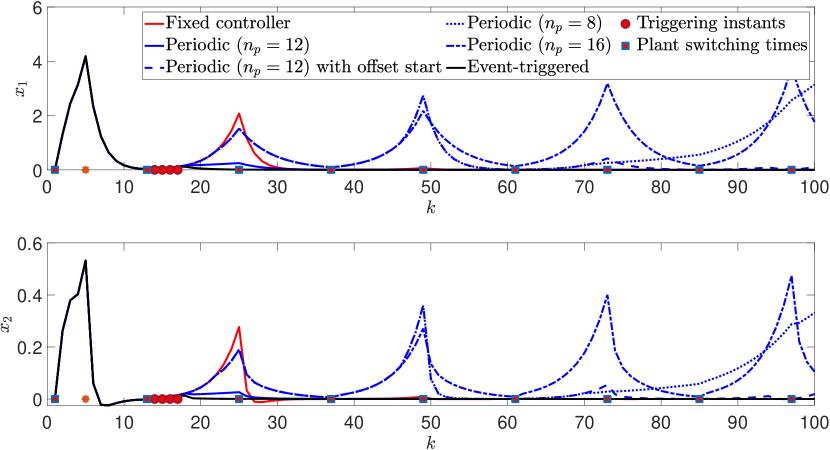
Figure 1: Closed-loop state response of (67) with different controllers (fixed, adaptive periodic time-triggered, and adaptive event-triggered).

The results in Figure 1 show that the event-triggered scheme (solid black curve) outperforms all the other schemes at regulating the system around the origin. From the reported triggering instants (cross markers) it can be seen that the scheme only triggers after the plant first switch has occurred (cross markers denote the plant switches) and does this only using observed data. On the other hand, the time-triggered strategy shows low robustness to inexact choice of period and first triggering instant. Indeed, while the performance of the oracle case (solid blue curve) is only slightly worse than the even-triggered case, the other three cases all display undesired oscillations and, in some cases, non-convergent behaviours. Note that in this case the non-adaptive solution using $K_{0}$ (solid red curve) leads to a converging response after some initial transient.

We then also consider the case where the switch affects the second column of the input matrix not only by changing its sign but also by scaling it up, that is

$$\begin{array}[]{rlll}B(k)&=\begin{cases}\begin{bmatrix}0.5&1\\ 0.1&0.2\\ \end{bmatrix},&k\in[1+p(z-1),pz],z=2n+1,\vspace{0.1in}\\ \begin{bmatrix}0.5&-\ell 1\\ 0.1&-\ell 0.2\\ \end{bmatrix},&k\in[1+p(z-1),pz],z=2n,\\ \end{cases}\end{array}$$ (68)

where $\ell=2.5$. The time-triggered solutions show similar trends, thus we compare in Figure 2 the non-adaptive case based on $K_{0}$ with the event-triggered solution. The former now clearly shows diverging behaviour, whereas the response of the adaptive even-triggered controlled system is qualitatively unchanged with respect to the case with $\ell=1$ (which is reported for reference in Figure 2 with a black dashed line).

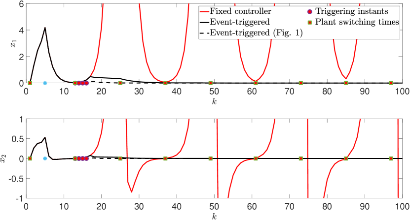
Figure 2: Closed-loop state response of the system with both sign switch and scaling change of the control matrix second column (68). Comparison between fixed and adaptive time-triggered controller.

Overall, these results show that the proposed event-triggered solution, without any prior knowledge of the time-variations, robustly addresses a challenging regulation problem where other more common approaches would fail or lack robustness.

8.3 Sinusoidal variations

We consider now the following perturbations to (66)

$$\begin{array}[]{rlll}A(k)&=\begin{bmatrix}1.1&0.1\\ 0.1&0.2\\ \end{bmatrix}\left(I_{2}+\delta_{a}\text{diag}(\cos{\frac{2\pi}{p}k},-\cos{\frac{2\pi}{p}k})\right),\vspace{0.1in}\\ B(k)&=B_{0}\;\forall k\in\mathbb{Z}_{\geq 0}\end{array}$$ (69)

with $\delta_{a}=0.8$. The input matrix is now constant and the state matrix undergoes a structured sinusoidal perturbation of period $p$ which determines a change up to $80\%$ for the diagonal values. Figure 3 shows the closed-loop the response of (69) with the event-triggered scheme for different values of $p$.

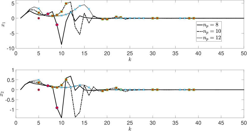
Figure 3: Closed-loop state response of system (69) for 3 values of $p$ controlled with the adaptive event-triggered controller.

The results show that in all cases the proposed controllers successfully regulate the system to the origin with a limited number of episodes (each triggering instant is denoted with a differently shaped marker on the corresponding curve). The simulation was carried out until $k=100$ but the $x$-axis is stopped before as all curves reached the origin and no further episode is triggered. The fixed controller $K_{0}$ led to unstable responses for all the considered values of $p$.

9 Conclusions

This work addresses the problem of data-based stabilization of linear time-varying systems by on-line adaptation of the feedback gain. We propose a hybrid systems framework, which casts the adaptation as a jump in the dynamics triggered by events depending on some relevant closed-loop properties. The control design uses robust LMI conditions based on the most recently collected data to guarantee a Lyapunov-like property for all the systems sufficiently close to those that generated the data. The formulation allows the problem of establishing how and when adaptation should take place to be formally addressed, and a closed-loop analysis of the resulting nonlinear feedback loop to be performed using nonlinear control techniques. We establish sufficient conditions under which the interconnection achieves different notions of stability, and we provide examples where this can be established under conditions related to the time-variations of the plant. Besides studying different triggering conditions, open research questions include the effect of both process and measurement noise, the addition of exploratory signals to guarantee richness of the collected data and the extension to nonlinear plants.

Appendix: Proof of Lemma 4

The proof is organized as follows. Under the full raw rank assumption on $Z$, we first prove the “only if” part of item (i), which we then exploit to show that item (ii) holds. We finally invoke item (ii) to establish the “if” part of item (i). We finally relax the assumption on the rank of $Z$ and prove items (iii) and (iv).

Item (i) (“only if”). Let $R:=Z^{\top}M^{-1}Z$. Since $Z$ has full row rank by assumption, $M$ is positive definite and therefore $R\succeq 0$. On the other hand,

$$\begin{array}[]{rlllll}\Delta&=XZ^{\top}M^{-1}ZX^{\top}-XX^{\top}+F\\ &=XRX^{\top}-XX^{\top}+F\\ &=X(R-I_{T})X^{\top}+F.\end{array}$$ (70)

We first show that

$$\Delta=\widetilde{D}(\mathrm{d},M_{A},M_{B})(R-I_{T})\widetilde{D}(\mathrm{d},M_{A},M_{B})^{\top}+F,\,\forall M_{A},M_{B}.$$ (71)

For this, we fix $M_{A}\in\mathbb{R}^{n_{x}\times n_{x}}$ and $M_{B}\in\mathbb{R}^{n_{u}\times n_{x}}$ and observe that (28), (32) and (34) yield

$$\begin{array}[]{rlllll}X&=M_{A}\widehat{X}(q)+M_{B}U-\widetilde{D}(\mathrm{d},M_{A},M_{B})\\ &=[M_{B}\,\,M_{A}]Z-\widetilde{D}(\mathrm{d},M_{A},M_{B}).\end{array}$$ (72)

Hence

$$\begin{array}[]{ll}(R-I_{T})X^{\top}=\\ -(R-I_{T})\widetilde{D}(\mathrm{d},M_{A},M_{B})^{\top}+(R-I_{T})Z^{\top}[M_{B}\,M_{A}]^{\top}.\end{array}$$ (73)

By definition of $R$ and $M$, we note that

$$\begin{array}[]{rlllll}\begin{aligned} &(R-I_{T})Z^{\top}[M_{B}\,M_{A}]^{\top}=\Big{(}Z^{\top}M^{-1}Z-I_{T}\Big{)}Z^{\top}[M_{B}\,M_{A}]^{\top}\\ &=Z^{\top}\Big{(}M^{-1}ZZ^{\top}-I_{T}\Big{)}[M_{B}\,M_{A}]^{\top}\\ &=Z^{\top}\Big{(}M^{-1}M-I_{T}\Big{)}[M_{B}\,M_{A}]^{\top}=0.\end{aligned}\end{array}$$ (74)

Consequently, in view of (73), we deduce $(R-I_{T})X^{\top}=-(R-I_{T})\widetilde{D}(\mathrm{d},M_{A},M_{B})^{\top}$, and thus, as $R$ is symmetric,

$$X(R-I_{T})=-\widetilde{D}(\mathrm{d},M_{A},M_{B})(R-I_{T}).$$ (75)

Applying these last two equations to (70) yields (71) as $M_{A}$ and $M_{B}$ have been arbitrarily selected.

We take $\left[M_{B}\,\,M_{A}\right]^{\top}\in\mathcal{E}(\mathrm{d},F)$, where the existence of such a pair is justified by the assumed non-emptiness of $\mathcal{E}(\mathrm{d},F)$. By (71),

$$\begin{array}[]{rlllll}\Delta&=\widetilde{D}(\mathrm{d},M_{A},M_{B})(R-I_{T})\widetilde{D}(\mathrm{d},M_{A},M_{B})^{\top}+F\\ &\succeq-\widetilde{D}(M_{A},M_{A})\widetilde{D}(\mathrm{d},M_{A},M_{B})^{\top}+F\succeq 0,\end{array}$$ (76)

where we first use that $R\succeq 0$ and then the fact that $\widetilde{D}(\mathrm{d},M_{A},M_{B})\widetilde{D}(\mathrm{d},M_{A},M_{B})^{\top}\preceq F$ as $[M_{B}\,M_{A}]^{\top}\in\mathcal{E}(\mathrm{d},F)$. We have proved the desired result.

Item (ii). Let $M_{A}$ and $M_{B}$ be of compatible dimensions, we have by (32) and (34)

$$\begin{array}[]{rllll}\widetilde{D}(\mathrm{d},M_{A},M_{B})&=&\left[M_{B}\,\,M_{A}\right]Z-X.\end{array}$$ (77)

Therefore

$$\begin{array}[]{rlllll}&\widetilde{D}(\mathrm{d},M_{A},M_{B})\widetilde{D}(\mathrm{d},M_{A},M_{B})^{\top}\preceq F\\ \Leftrightarrow&\left(\left[M_{B}\,\,M_{A}\right]Z-X\right)\left(Z^{\top}\left[M_{B}\,\,M_{A}\right]^{\top}-X^{\top}\right)\preceq F\\ \Leftrightarrow&\left[M_{B}\,\,M_{A}\right]ZZ^{\top}\left[M_{B}\,\,M_{A}\right]^{\top}-\left[M_{B}\,\,M_{A}\right]ZX^{\top}\\ &\hfill-XZ^{\top}\left[M_{B}\,\,M_{A}\right]^{\top}+XX^{\top}\preceq F.\\ \end{array}$$ (78)

Define now $N:=-ZX^{\top}$ and $C:=XX^{\top}-F$. Hence $\widetilde{D}(\mathrm{d},M_{A},M_{B})\widetilde{D}(\mathrm{d},M_{A},M_{B})^{\top}\preceq F$ if and only if $\left[M_{B}\,\,M_{A}\right]^{\top}\in\widetilde{\mathcal{E}}(\mathrm{d},F)$ where

$$\widetilde{\mathcal{E}}(\mathrm{d},F) :=\Big{\{}\widetilde{Z}\,:\,\widetilde{Z}^{\top}M\widetilde{Z}+\widetilde{Z}^{\top}N+N^{\top}\widetilde{Z}+C\preceq 0\Big{\}}.$$ (79)

This shows $\mathcal{E}(\mathrm{d},F)=\widetilde{\mathcal{E}}(\mathrm{d},F)$. Note that showing this equality does not require any assumption on the rank of $Z$. When $Z$ has full row rank, then $M\succ 0$ and $N^{\top}M^{-1}N-C=\Delta\succeq 0$ from item (i) because $\left[M_{B}\,\,M_{A}\right]^{\top}\in\mathcal{E}(\mathrm{d},F)$. Therefore $\widetilde{\mathcal{E}}(\mathrm{d},F)$ is a matrix ellipsoidal. The desired result is then obtained by noticing that the ellipsoidal set $\widehat{\mathcal{E}}(\mathrm{d},F)$ is equivalent to $\widetilde{\mathcal{E}}(\mathrm{d},F)$ in (37) by taking $Z_{c}=-M^{-1}N$ and $\Delta=N^{\top}M^{-1}N-C$.

Item (i) (“if”). If $\Delta\in\mathbb{S}^{n_{x}}_{\succeq 0}$, then set $\widehat{\mathcal{E}}(\mathrm{d},F)$ is non-empty as $Z_{c}\in\widehat{\mathcal{E}}(\mathrm{d},F)$. By item (ii), the equivalence (36) holds and thus set $\mathcal{E}(\mathrm{d},F)$ is also non-empty.

Item (iii). Define $\widetilde{V}^{\top}\in\mathbb{R}^{m\times n_{x}+n_{u}}$ and $\widetilde{W}^{\top}\in\mathbb{R}^{(n_{x}+n_{u}-m)\times n_{x}+n_{u}}$ as in the statement of the lemma. Using the range-null space decomposition, we can write any matrix $\widetilde{Z}\in\mathbb{R}^{(n_{x}+n_{u})\times n_{x}}$ as

$$\widetilde{Z}^{\top}=\widetilde{P}\widetilde{W}^{\top}+\widetilde{Q}\widetilde{V}^{\top}=\left[\widetilde{P}\,\,\widetilde{Q}\right]\begin{bmatrix}\widetilde{W}^{\top}\\ \widetilde{V}^{\top}\end{bmatrix}$$

for appropriate matrices $\widetilde{P},\widetilde{Q}$. Recall moreover that the equivalence $\mathcal{E}(\mathrm{d},F)=\widetilde{\mathcal{E}}(\mathrm{d},F)$ in item (ii) does not require any assumption on the rank of $Z$. For these reasons, we can write

$$\widetilde{\mathcal{E}}(\mathrm{d},F):=\Big{\{}\widetilde{Z}\,:\,\widetilde{Z}^{\top}M\widetilde{Z}+\widetilde{Z}^{\top}N+N^{\top}\widetilde{Z}+C\preceq 0\Big{\}},$$ (80)

$$=\Big{\{}[\widetilde{P}\,\,\widetilde{Q}]\in\mathbb{R}^{(n_{x}+n_{u})\times n_{x}}\,:\,[\widetilde{P}\;\;\widetilde{Q}]\begin{bmatrix}\widetilde{W}^{\top}\\ \widetilde{V}^{\top}\end{bmatrix}M(\star)+$$

$$\quad\quad+[\widetilde{P}\;\;\widetilde{Q}]\begin{bmatrix}\widetilde{W}^{\top}\\ \widetilde{V}^{\top}\end{bmatrix}N+N^{\top}(\star)+C\preceq 0\Big{\}},$$

$$=\Big{\{}[\widetilde{P}\,\,\widetilde{Q}]\,:\,\widetilde{Q}\widetilde{M}\widetilde{Q}^{\top}+\widetilde{Q}\widetilde{N}+\widetilde{N}^{\top}\widetilde{Q}^{\top}+C\preceq 0\Big{\}},$$

where we have defined $\widetilde{M}:=\widetilde{V}^{\top}M\widetilde{V}$ and $\widetilde{N}:=\widetilde{V}^{\top}N$. Note that $\widetilde{M}$ has full row rank by choice of $\widetilde{V}$, and the conditions defining (80) do not depend on $\widetilde{P}$. We can thus use the same arguments of item (ii) to show that $\widetilde{\mathcal{E}}(\mathrm{d},F)$ is equivalent to

$$\widehat{\mathcal{E}}(\mathrm{d},F):=\big{\{}[\widetilde{P}\,\,\widetilde{Q}]\,:\,(\widetilde{Q}^{\top}-\widetilde{Z}_{c})^{\top}\widetilde{M}(\widetilde{Q}^{\top}-\widetilde{Z}_{c})\preceq\widetilde{\Delta}\big{\}}$$ (81)

by taking $\widetilde{Z}_{c}=-\widetilde{M}^{-1}\widetilde{N}$ and $\widetilde{\Delta}=\widetilde{N}^{\top}\widetilde{M}^{-1}\widetilde{N}-C$, where the latter expression coincides with (38). This shows $\mathcal{E}(\mathrm{d},F)=\widetilde{\mathcal{E}}(\mathrm{d},F)=\widehat{\mathcal{E}}(\mathrm{d},F)$ and thus (81) characterizes $\mathcal{E}(\mathrm{d},F)$ when $Z$ is not full row rank. Moreover, following the same reasoning of item (ii), this set is non-empty if and only if $\widetilde{\Delta}\succeq 0$. Note that this set is either empty or unbounded, because if $[\widetilde{P}\,\,\widetilde{Q}]\in\widetilde{\mathcal{E}}(\mathrm{d},F)$ for $\widetilde{P},\widetilde{Q}$, then clearly $[\widehat{P}\,\,\widetilde{Q}]\in\widetilde{\mathcal{E}}(\mathrm{d},F)$ for all $\widehat{P}$ of compatible dimensions.

Appendix: Proof of Proposition 2

We rely on the next intermediate lemma.

Lemma 7

Under the conditions of Proposition 2, for any $\varepsilon\in\mathbb{R}_{\geq 0}$, $\left[M_{B}\,\,M_{A}\right]^{\top}\in\mathcal{E}(\mathrm{d},F+\varepsilon S^{-1})$ implies $S-(M_{A}+M_{B}K)^{\top}\Big{(}\star\Big{)}^{-1}(M_{A}+M_{B}K)\succ 0$, with $S=(\widehat{X}Y)^{-1}$, $\star=S^{-1}-H+(1+\varsigma^{-1})(F+\varepsilon S^{-1})$. $\Box$

Proof: The proof follows the main steps of [3, proof of Theorem 5] adapted to the LTV context of this work. Let $\mathrm{d}\in\mathcal{S}_{\mathrm{d}}$ be such that (40) holds. We restrict the controller $K$ we search over to be of the form

$$\begin{array}[]{rllll}\left[\begin{matrix}K\\ I_{n_{x}}\end{matrix}\right]&=&\left[\begin{matrix}U\\ \widehat{X}\end{matrix}\right]G,\end{array}$$ (82)

where $G\in\mathbb{R}^{T\times n_{x}}$. Let $M_{A}\in\mathbb{R}^{n_{x}\times n_{x}}$ and $M_{B}\in\mathbb{R}^{n_{u}\times n_{x}}$, we have from (82)

$$\begin{array}[]{rllll}M_{A}+M_{B}K&=&\big{[}\begin{matrix}M_{B}&M_{A}\end{matrix}\big{]}\left[\begin{matrix}K\\ I_{n_{x}}\end{matrix}\right]\vspace{0.2cm}\\ &=&\big{[}\begin{matrix}M_{B}&M_{A}\end{matrix}\big{]}\left[\begin{matrix}U\\ \widehat{X}\end{matrix}\right]G\\ &=&(M_{A}\widehat{X}+M_{B}U)G.\end{array}$$ (83)

We deduce from (32) and (40) that

$$\begin{array}[]{rllll}M_{A}+M_{B}K=(X+\widetilde{D}(q,M_{A},M_{B}))G.\end{array}$$ (84)

To ease the notation, we omit in the reminder the arguments of $\widetilde{D}$ unless necessary. The first main step of the proof consists in showing the existence of $P\in\mathbb{S}^{n_{x}}_{\succ 0}$ and $\widetilde{W}\in\mathbb{S}^{n_{x}}$ such that

$$\begin{array}[]{rlllll}(X+\widetilde{D})GPG^{\top}(X+\widetilde{D})^{\top}-P&\prec&-\widetilde{W}.\end{array}$$ (85)

To this end, we define $Y:=GP$. Then, from the second block row of (82) it follows that

$$P=\widehat{X}GP=\widehat{X}Y.$$ (86)

Using the second LMI in (41), this shows immediately that $\widehat{X}Y=P\succ 0$. Indeed, by Schur complement of the second LMI in (41), $\widehat{X}Y-Y^{\top}Y\succ 0$, and thus $\widehat{X}Y\succ Y^{\top}Y\succeq 0$.

Using the invertibility of $P$, we can write

$$GPG^{\top}=Y(\widehat{X}Y)^{-1}Y^{\top}.$$ (87)

Leveraging Young’s inequality we know that for any real matrices of compatible dimensions $M_{1},M_{2},N$ with $N\succ 0$ and any $\epsilon\in\mathbb{R}_{>0}$, $M_{1}NM_{2}^{\top}+M_{2}NM_{1}^{\top}\preceq\epsilon M_{1}NM_{1}^{\top}+\epsilon^{-1}M_{2}NM_{2}^{\top}$. We derive, by taking $M_{1}=XY(\widehat{X}Y)^{-1}$, $N=\widehat{X}Y$, $M_{2}=\widetilde{D}Y(\widehat{X}Y)^{-1}$ and $\epsilon=\varsigma$, and (86) and (87)

$$\begin{array}[]{llllll}(X+\widetilde{D})GPG^{\top}(X+\widetilde{D})^{\top}-P\\ \quad=(X+\widetilde{D})Y(\widehat{X}Y)^{-1}Y^{\top}(X+\widetilde{D})^{\top}-\widehat{X}Y\\ \quad\preceq(1+\varsigma)XY(\widehat{X}Y)^{-1}(XY)^{\top}\\ \quad\quad+(1+\varsigma^{-1})\widetilde{D}Y(\widehat{X}Y)^{-1}(\widetilde{D}Y)^{\top}-\widehat{X}Y.\end{array}$$ (88)

By Schur complement of the second LMI in (41), $I_{T}-Y(\widehat{X}Y)^{-1}Y^{\top}\succ 0$, equivalently

$$I_{T}\succ Y(\widehat{X}Y)^{-1}Y^{\top}.$$ (89)

As a consequence,

$$\begin{array}[]{llllll}(X+\widetilde{D})GPG^{\top}(X+\widetilde{D})^{\top}-P\\ \quad\quad\quad\quad\preceq(1+\varsigma)XY(\widehat{X}Y)^{-1}(XY)^{\top}\\ \quad\quad\quad\quad\quad+(1+\varsigma^{-1})\widetilde{D}\widetilde{D}^{\top}-\widehat{X}Y.\end{array}$$ (90)

Let $F\in\mathbb{S}_{\succ 0}^{n_{x}}$ be such that $F\prec\frac{\varsigma}{1+\varsigma}H$ and $\varepsilon\in\mathbb{R}_{\geq 0}$. Take $\big{[}M_{B}\,\,M_{A}\big{]}^{\top}\in\mathcal{E}(\mathrm{d},F+\varepsilon P)$, it holds that $\widetilde{D}(M_{A},M_{B})\widetilde{D}(q,M_{A},M_{B})^{\top}\preceq F+\varepsilon P$ and thus

$$(X+\widetilde{D})GPG^{\top}(X+\widetilde{D})^{\top}-P\preceq(1+\varsigma)XY(\widehat{X}Y)^{-1}(XY)^{\top}$$ (91)

$$+(1+\varsigma^{-1})(F+\varepsilon P)-\widehat{X}Y=:\Theta.$$

By Schur complement of the first LMI in (41), $\widehat{X}Y-\varsigma XX^{\top}-H-XY(\widehat{X}Y)^{-1}(XY)^{\top}\succ 0$, which we rewrite as, in view of the definition of $\Theta$ in (91), $(1+\varsigma)XY(\widehat{X}Y)^{-1}(XY)^{\top}+(1+\varsigma^{-1})(F+\varepsilon P)-\Theta-\varsigma XX^{\top}-H-XY(\widehat{X}Y)^{-1}(XY)^{\top}\succ 0$. Equivalently,

$$\begin{array}[]{rlllll}\Theta&\prec&\varsigma XY(\widehat{X}Y)^{-1}(XY)^{\top}+(1+\varsigma^{-1})(F+\varepsilon P)\\ &&-\varsigma XX^{\top}-H.\end{array}$$ (92)

From (89) we obtain

$$\begin{array}[]{rlllll}\Theta&\prec&(1+\varsigma^{-1})(F+\varepsilon P)-H.\end{array}$$ (93)

Define $W=H-(1+\varsigma^{-1})F$ and observe that $W\succ 0$ as $F\prec\frac{\varsigma}{1+\varsigma}H$. We can then write

$$\begin{array}[]{rlllll}\Theta&\prec&-W+(1+\varsigma^{-1})\varepsilon P=:-\widetilde{W}.\end{array}$$ (94)

Piecing together (91) and (94) yields (85).

Now, rewrite (85) as $(X+\widetilde{D})GPG^{\top}(X+\widetilde{D})^{\top}-(P-\widetilde{W})\prec 0$ and do a Schur complement to obtain

$$\left[\begin{matrix}P-\widetilde{W}&(X+\widetilde{D})G\\ \star&P^{-1}\end{matrix}\right]\succ 0.$$ (95)

Considering the other Schur complement of the matrix above, we get

$$P^{-1}-((X+\widetilde{D})G)^{\top}(P-\widetilde{W})^{-1}(X+\widetilde{D})G\succ 0,$$ (96)

note that $P-\widetilde{W}\in\mathbb{S}^{n_{x}}_{\succ 0}$ by definition of $\widetilde{W}$ and because from the first LMI in (41) we have $P\succ H$, as principal submatrices of positive definite matrices are positive definite.

Let $S=P^{-1}$, $\varepsilon\in\mathbb{R}_{\geq 0}$ and $\big{[}M_{B}\,\,M_{A}\big{]}^{\top}\in\mathcal{E}(\mathrm{d},F+\varepsilon S^{-1})$, by (96) and the definition of $\widetilde{W}$, $S-(M_{A}+M_{B}K)^{\top}(S^{-1}-W+(1+\varsigma^{-1})\varepsilon S^{-1})^{-1}(M_{A}+M_{B}K)\succ 0$. We have obtained the desired result. $\blacksquare$

We are now ready to prove Proposition 2. Let $\varepsilon\in\mathbb{R}_{\geq 0}$, $\left[M_{B}\,\,M_{A}\right]^{\top}\in\mathcal{E}(\mathrm{d},F+\varepsilon S^{-1})$ with $S$ as in Lemma 7, and $x\in\mathbb{R}^{n_{x}}$. By Lemma 7, $x^{\top}(M_{A}+M_{B}K)^{\top}(S^{-1}-\widetilde{W})^{-1}(M_{A}+M_{B}K)x-x^{\top}Sx\leq 0$ with $\widetilde{W}=H-(1+\varsigma^{-1})(F+\varepsilon S^{-1})$ as in the proof of Lemma 7, which we rewrite as

$$\begin{array}[]{llllll}x^{\top}(M_{A}+M_{B}K)^{\top}S(M_{A}+M_{B}K)x-x^{\top}Sx\leq\\ -x^{\top}(M_{A}+M_{B}K)^{\top}\big{[}\big{(}S^{-1}-\widetilde{W}\big{)}^{-1}-S\big{]}(M_{A}+M_{B}K)x.\end{array}$$ (97)

By taking $V(x,S)=x^{\top}Sx$ and $Q:=\big{(}S^{-1}-\widetilde{W}\big{)}^{-1}-S$, we obtain

$$V((M_{A}+M_{B}K)x,S)-V(x,S)\leq$$ (98)

$$\quad-x^{\top}(M_{A}+M_{B}K)^{\top}Q(M_{A}+M_{B}K)x.$$

We show next that there exists $\lambda(\varepsilon)\in(-1,+\infty)$ such that $Q\succeq\lambda(\varepsilon)S$. We note that $a=\max\big{\{}a^{\prime}\in\mathbb{R}_{\geq 0}\,:\,a^{\prime}S^{-1}\preceq W\big{\}}$ belongs to $(0,1)$ as $S,W\in\mathbb{S}^{n_{x}}_{\succ 0}$ and $P\succ H$ (from (41)) implies $S^{-1}-W\succ 0$. Take

$$\lambda(\varepsilon)=\frac{a-(1+\varsigma^{-1})\varepsilon}{1-a+(1+\varsigma^{-1})\varepsilon},$$ (99)

where the denominator is positive because $\varepsilon\in\mathbb{R}_{\geq 0}$, $a\in(0,1)$ and $\varsigma>0$. Moreover, it holds

$$\lambda(\varepsilon)+1 =\frac{1}{1-a+(1+\varsigma^{-1})\varepsilon}>0.$$ (100)

This proves that $\lambda(\varepsilon)\in(-1,+\infty)$. To show $Q\succeq\lambda(\varepsilon)S$, observe that

$$Q\succeq\lambda(\varepsilon)S \Leftrightarrow\left(S^{-1}-W+(1+\varsigma^{-1})\varepsilon S^{-1}\right)^{-1}\!-\!S\succeq\lambda(\varepsilon)S$$ (101)

$$\Leftrightarrow S^{-1}\!-\!W\!+\!(1+\varsigma^{-1})\varepsilon S^{-1}\!\!\preceq\tfrac{1}{1+\lambda(\varepsilon)}S^{-1}$$

$$\Leftrightarrow\big{(}1-\tfrac{1}{1+\lambda(\varepsilon)}+(1+\varsigma^{-1})\varepsilon\big{)}S^{-1}\preceq W$$

$$\Leftrightarrow\big{(}\tfrac{\lambda(\varepsilon)}{1+\lambda(\varepsilon)}+(1+\varsigma^{-1})\varepsilon\big{)}S^{-1}\preceq W.$$

By (99) and (100), $\tfrac{\lambda(\varepsilon)}{1+\lambda(\varepsilon)}+(1+\varsigma^{-1})\varepsilon=a$ therefore $Q\succeq\lambda(\varepsilon)S\Leftrightarrow aS^{-1}\preceq W$. The last inequality holds by definition of $a$. We deduce that $Q\succeq\lambda(\varepsilon)S$. We use this property together with (98) to derive that for all $\left[M_{B}\,\,M_{A}\right]^{\top}\in\mathcal{E}(\mathrm{d},F+\varepsilon S^{-1})$ $V((M_{A}+M_{B}K)x,S)-V(x,S)\leq-\lambda(\varepsilon)V((M_{A}+M_{B}K)x,S)$ and thus, by (100) $V((M_{A}+M_{B}K)x,S)\leq\frac{1}{1+\lambda(\varepsilon)}V(x,S)=(1-a+(1+\varsigma^{-1})\varepsilon)V(x,S)$. The desired result holds with $a_{1}=1-a\in(0,1)$ and $a_{2}=1+\varsigma^{-1}$.

References

[] Andrea Iannelli (Member, IEEE) is an Assistant Professor in the Institute for Systems Theory and Automatic Control at the University of Stuttgart. He completed his B.Sc. and M.Sc. degrees in Aerospace Engineering at the University of Pisa and received his PhD from the University of Bristol. He was also a postdoctoral researcher in the Automatic Control Laboratory at ETH Zurich. His main research interests are at the intersection of control theory, optimization, and learning, with a particular focus on robust and adaptive control, uncertainty quantification, and sequential decision-making. [] Romain Postoyan (Senior Member, IEEE) received the “Ingénieur” degree in Electrical and Control Engineering from ENSEEIHT (France) in 2005. He obtained the M.Sc. by Research in Control Theory & Application from Coventry University (United Kingdom) in 2006 and the Ph.D. in Control Engineering from Université Paris-Sud (France) in 2009. In 2010, he was a research assistant at the University of Melbourne (Australia). Since 2011, he is a CNRS researcher at CRAN (Nancy, France).

References

- [1] R. Sanfelice and A. Teel, “Dynamical properties of hybrid systems simulators,” Automatica, vol. 46, no. 2, pp. 239–248, 2010.
- [2] W. Heemels, K. Johansson, and P. Tabuada, “An introduction to event-triggered and self-triggered control,” in IEEE Conference on Decision and Control, pp. 3270–3285, 2012.
- [3] C. De Persis and P. Tesi, “Formulas for data-driven control: Stabilization, optimality, and robustness,” IEEE Trans. on Automatic Control, vol. 65, no. 3, pp. 909–924, 2020.
- [4] H. van Waarde, M. Camlibel, and M. Mesbahi, “From noisy data to feedback controllers: Nonconservative design via a matrix S-lemma,” IEEE Trans. on Automatic Control, vol. 67, no. 1, pp. 162–175, 2020.
- [5] J. Berberich, C. Scherer, and F. Allgöwer, “Combining prior knowledge and data for robust controller design,” IEEE Trans. on Automatic Control, vol. 68, no. 8, pp. 4618–4633, 2023.
- [6] M. Rotulo, C. De Persis, and P. Tesi, “Online learning of data-driven controllers for unknown switched linear systems,” Automatica, vol. 145, p. 110519, 2022.
- [7] S. Liu, K. Chen, and J. Eising, “Online data-driven adaptive control for unknown linear time-varying systems,” in IEEE Conference on Decision and Control, pp. 8775–8780, 2023.
- [8] B. Nortmann and T. Mylvaganam, “Direct data-driven control of linear time-varying systems,” IEEE Trans. on Automatic Control, vol. 68, no. 8, pp. 4888–4895, 2023.
- [9] M. Mazo, A. Anta, and P. Tabuada, “An ISS self-triggered implementation of linear controllers,” Automatica, vol. 46, no. 8, pp. 1310–1314, 2010.
- [10] X. Wang and M. Lemmon, “On event design in event-triggered feedback systems,” Automatica, vol. 47, no. 10, pp. 2319–2322, 2011.
- [11] A. Maass, W. Wang, D. Nešić, R. Postoyan, and W. Heemels, “Event-triggered control through the eyes of a hybrid small-gain theorem,” IEEE Trans. on Automatic Control, vol. 68, no. 10, pp. 5906–5921, 2023.
- [12] C. De Persis, R. Postoyan, and P. Tesi, “Event-triggered control from data,” IEEE Trans. on Automatic Control, vol. available on-line, 2023.
- [13] W.-L. Qi, K.-Z. Liu, R. Wang, and X.-M. Sun, “Data-driven -stability analysis for dynamic event-triggered networked control systems: A hybrid system approach,” IEEE Trans. on Industrial Electronics, vol. 70, no. 6, pp. 6151–6158, 2022.
- [14] X. Wang, J. Berberich, J. Sun, G. Wang, F. Allgöwer, and J. Chen, “Model-based and data-driven control of event-and self-triggered discrete-time linear systems,” IEEE Trans. on Cyb., vol. 53, no. 9, pp. 6066 – 6079, 2023.
- [15] R. Goebel, R. Sanfelice, and A. Teel, Hybrid Dynamical Systems. Princeton University Press, Princeton, U.S.A., 2012.
- [16] H. van Waarde, J. Eising, H. Trentelman, and M. Camlibel, “Data informativity: a new perspective on data-driven analysis and control,” IEEE Trans. on Automatic Control, vol. 65, no. 11, pp. 4753–4768, 2020.
- [17] J. C. Willems, P. Rapisarda, I. Markovsky, and B. D. Moor, “A note on persistency of excitation,” Syst. & Contr. Lett., vol. 54, no. 4, pp. 325–329, 2005.
- [18] A. Girard, “Dynamic triggering mechanisms for event-triggered control,” IEEE Trans. on Automatic Control, vol. 60, no. 7, pp. 1992–1997, 2015.
- [19] S. Benahmed, R. Postoyan, M. Granzotto, L. Buşoniu, J. Daafouz, and D. Nešić, “Stability analysis of optimal control problems with time-dependent costs,” Automatica, vol. 157, p. 111272, 2023.
- [20] A. Bisoffi, C. De Persis, and P. Tesi, “Trade-offs in learning controllers from noisy data,” Systems & Control Letters, vol. 154, 2021.
- [21] A. Bisoffi, C. De Persis, and P. Tesi, “Data-driven control via Petersen’s lemma,” Automatica, vol. 145, p. 110537, 2022.
- [22] D. Borgers, V. Dolk, G. Dullerud, A. Teel, and W. Heemels, “Time-regularized and periodic event-triggered control for linear systems,” in Control Subject to Computational and Communication Constraints, pp. 121–149, Springer, 2018.
- [23] M. Abdelrahim, R. Postoyan, J. Daafouz, and D. Nešić, “Robust event-triggered output feedback controllers for nonlinear systems,” Automatica, vol. 75, pp. 96–108, 2017.
- [24] P. Tallapragada and N. Chopra, “Event-triggered dynamic output feedback control for LTI systems,” in IEEE Conference on Decision and Control, Maui, U.S.A., pp. 6597–6602, 2012.
- [25] W. Wang, D. Nešić, R. Postoyan, I. Shames, and W. Heemels, “State-feedback event-holding control for nonlinear systems,” in IEEE Conf. on Decision and Control, Nice, France, pp. 1650–1655, 2019.
- [26] M. ApS, The MOSEK optimization toolbox for MATLAB manual. Version 9.0., 2019.
[![[Uncaptioned image]](/html/2405.14426/assets/x4.png) ]