The interplay between liquid-liquid and ferroelectric phase transitions in supercooled water

Abstract

The distinctive characteristics of water, evident in its thermodynamic anomalies, have implications across disciplines from biology to geophysics. Considered a valid hypothesis to rationalize its unique properties, a liquid-liquid phase transition in water below the freezing point, in the so-called supercooled regime, has nowadays been observed in several molecular dynamics simulations and is being actively researched experimentally. In this work, we highlight novel and far-reaching implications of water: the interplay between the liquid-liquid and a ferroelectric phase transition. Our results are based on the analysis of extensive molecular dynamics simulations and are explained in the context of a classical density functional theory in mean-field approximation valid for a polar liquid, where dipolar interaction is treated perturbatively. The theory underpins the potential role of ferroelectricity in promoting the liquid-liquid phase transition, being the density-polarization coupling inherent in the dipolar interaction potential. The existence of ferroelectric order in supercooled low-density liquid water is confirmed by the observation in molecular dynamics simulations of collective modes in space-time polarization correlation functions, traceable to spontaneous breaking of continuous rotational symmetry. Our work sheds light on water’s supercooled behavior and opens the door to new experimental investigations of the static and dynamic behavior of water’s polarization.

The identification of equilibrium water’s thermodynamic anomalies, notably density maximum at 277 K, compressibility, and specific heat minima around 310 K and 280 K, respectively [1], has immediately sparked broad scientific interest. A first-order liquid-liquid phase transition (LLPT) between a high-density liquid (LDL) and a low-density liquid (HDL) in the supercooled regime, was proposed [2] to explain equilibrium water’s anomalies and polyamorphism [3]. The first observation of HDL and LDL water in molecular dynamics (MD) simulations is reported in Ref. [2]. Recently, extensive MD simulations in realistic [4], as well as ab initio neural network [5], models of water have clearly supported the first-order LLPT existence. The first-order LLPT line ends at a second-order critical point (CP). Despite experimental hints [9], direct evidence is challenging due to water’s crystallization tendency near the MD simulations-predicted CP. The Widom line (WL) [6], located in the pressure-temperature thermodynamic plane ($p$, $T$) region above CP but yet in the supercooled state, has been observed via both MD simulations [6] and experiments [7]. Crossing the WL from high $T$, water transforms smoothly from HDL-like to LDL-like configurations [6, 7], while the isothermal compressibility ($K_{T}$) reaches a local maximum [8]. Beyond density, different order parameters have been proposed to characterize the LLPT and elucidate its physical origin, mostly based on local structure geometry [10, 11, 12]. Recent insights, furthermore, indicate that varying degrees of topological order of hydrogen-bond network can distinguish HDL from LDL [13].

The notion of ferroelectric phase transition in supercooled water stems from a 1977 proposal by Stillinger [14], following the observation of proton ordering in certain ice polymorphs [15]. During the same years, measurements of the dielectric constant of supercooled water emulsions at ambient $p$ down to T=238 K [16, 17] revealed an increase in dielectric constant as $T$ decreased. Ref. [17] emphasized that this trend aligns with divergence at 228 K, close to the WL [8, 7], albeit with a rather small critical exponent. Although the idea persisted over the years - Refs. [18, 19] explore the potential ferroelectricity of equilibrium water - the connection between ferroelectricity and LLPT in supercooled water was not thoroughly examined. A series of papers [20, 21, 22] deal with the proposal of a model for the Gibbs free energy of supercooled water, aligning with a ferroelectric phase transition. Supercooled water, however, was assumed to be a mixture of HDL and LDL, with only LDL presumed to undergo a ferroelectric phase transition [22]. Beyond ices polymorphs [15], incipient ferroelectricity has been observed in confined water [23]. Interestingly, electrofreezing of water at ambient conditions was observed recently by ab initio MD simulations, highlighting the existence of an amorphous ferroelectric ice [24]. On the other hand, dielectric measurements reveal distinct differences in the dielectric properties of high- and low-density amorphous ices (HDA/LDA) [25]. Extrapolated from Ref. [25], LDA and HDA dielectric constant is respectively $\sim 10$ at $T\sim$ 130 K and $p$=4000 bars, and $\sim$ 130 at same $T$ and $p$=6000 bars.

Reanalyzing the water MD simulations in Ref. [4], a distinct correlation between density ($\rho$) and total polarization magnitude ($P$) emerges: while HDL retains paraelectric characteristics, the trend of LDL polarization suggests a ferroelectric character. A similar result was recently observed in ab initio deep neural-network simulations [29], thereby freeing it from possible dependencies on the MD simulation’s potential and water’s model. Ref. [29] furthermore shows how the different topology of HDL and LDL hydrogen-bond network reflect into different $P$. Taking a step further, the dipolar degrees of freedom drawing $P$ being involved in the water’s microscopic potential interaction, occurrence that distinguishes $P$ from other proposed order parameters [10, 11, 12], the hypothesis can be advanced that $P$ plays an active role in the LLPT. An analogy akin to that of ferroeleastic phase transition in crystals [26, 27] or liquid crystals [28] can be envisioned. On this trail, we firstly obtained from MD simulations the $P$-$\rho$ phase diagram in the ($p$, $T$) plane, secondly, starting from the microscopic interaction potential and treating the dipole interaction perturbatively, we developed a classical density functional theory (DFT) in a mean-field approximation. Unlike previous treatments, such as the notable examples in the Stockmayer fluid [30], our theory uniquely features the emergence of coupling between $P$, the order parameter, and $\rho$, stemming directly from the characteristics of dipole interaction. Our developments aim rationalizing the LLPT in water, modeled as a dipolar liquid. It does not exclude that different systems or different water models with different microscopic interactions [31] could led to the same phenomenology. A similar DFT approach could, in these cases, be applied.

0.1 Ferroelectric character of the LLPT in supercooled water

The temporal evolution of $P$ and polarization components along the three spatial directions, $P_{i}$, obtained from extensive MD simulations of TIP4P/Ice water lasting up to 40 $\mu$s of Ref. [4], reveals a clear correlation with $\rho$. MD simulations employed isothermal-isobaric (NpT) ensemble with $N=1000$ molecules. For additional details, refer to Section 1 and Ref. [4]. In the LDL phase, all $P_{i}$’s maintain a non-zero value, while in the HDL phase, they show large fluctuations around a zero mean value. At CP = $(\bar{p}_{c},\bar{T}_{c})$, where the temporal series shows the characteristic bimodal behavior, the $\rho$ fluctuation between LDL and HDL coincides with a transition in $P$ and $P_{i}$’s trend. Analyses covering several ($p$, $T$) points are in Supplementary Note I.

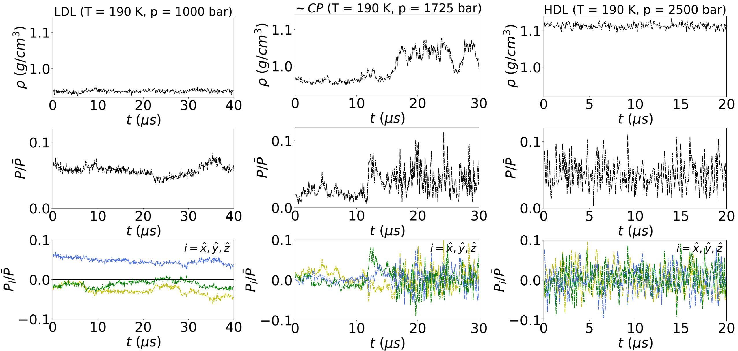
Figure 1: Temporal evolution of $\rho$ (top) $P$ (middle) and $P_{i}$ (bottom) across supercooled water in LDL phase (left), near CP (center) and in HDL phase (right) obtained from MD simulations suggests a paraelectric and ferroelectric character, respectively, for HDL and LDL. It is $\bar{P}=Nd$. The CP for TIP4P/Ice model has been evaluated [4] to be $(\bar{p}_{c}=1725\ bar,\bar{T}_{c}=188.6\ K)$.

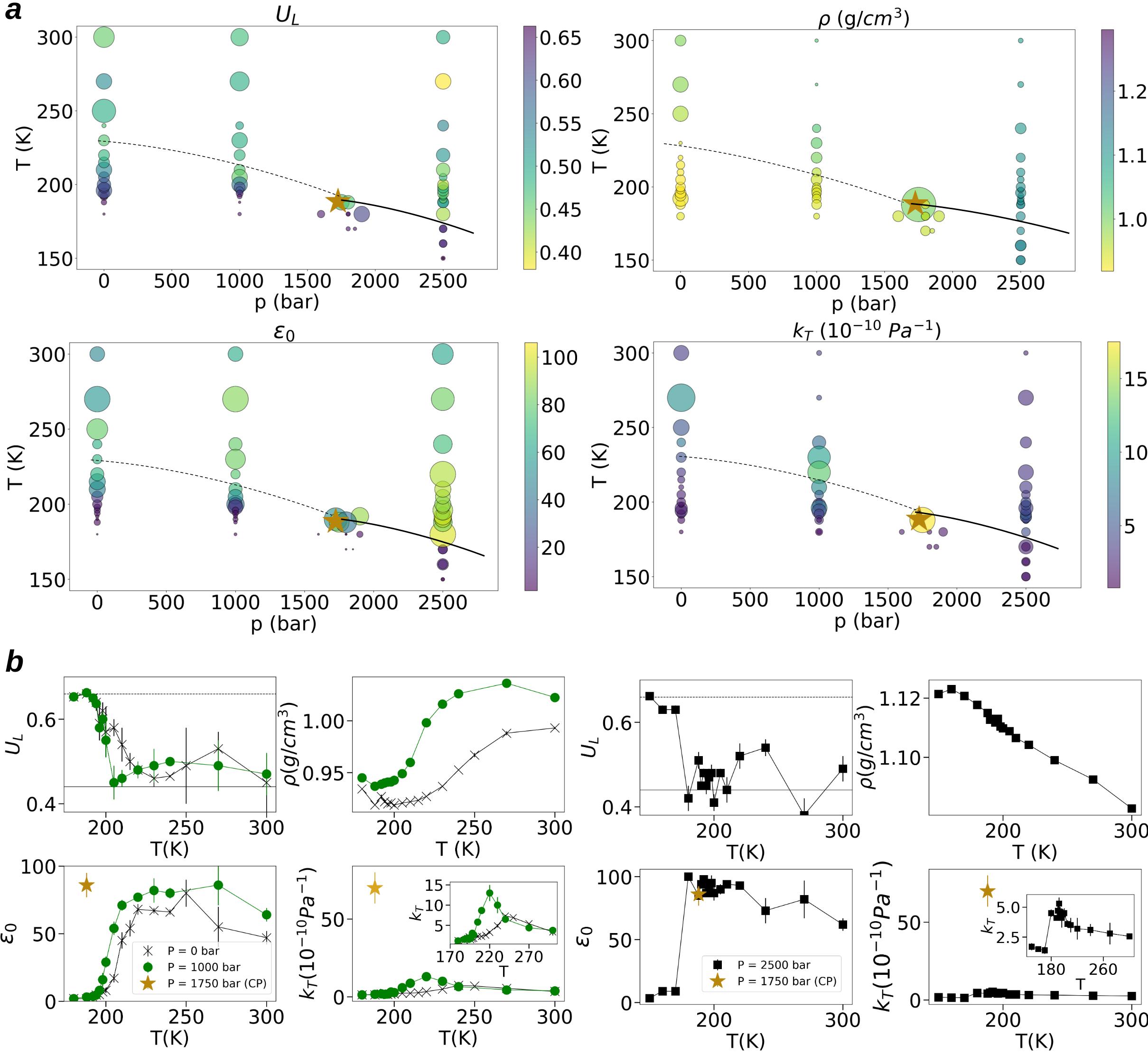
Figure 2: a, The figure depicts $U_{L}$, $\rho$, $\epsilon_{0}$, and $K_{T}$ across different points in the (T, p) plane obtained from MD simulations. The existence of the presumed ferroelectric phase transition accompanying the LLPT, as inferred from Fig. 1, is confirmed. Color scale represents the quantities value, symbol size is proportional to the associated error, obtained through block averaging. To improve clarity, the $K_{T}$ value closer to CP has been reduced by a factor of four. Full and dashed black lines serve as visual guidance, marking the first-order LLPT and WL, respectively. The star marks CP. b, $U_{L}$, $<\rho>$, $\epsilon_{0}$, and $K_{T}$ as functions of $T$ along constant-$p$ lines intersecting the WL ($p$=0 bar, 1000 bar, left) and the first-order LLPT line ($p$=2500 bar, right). The values of each quantity at CP are marked by a star. A gradual change is observed in $U_{L}$ and $\rho$ when crossing the WL, while a sudden shift in $U_{L}$ occurs at the first-order LLPT. line.

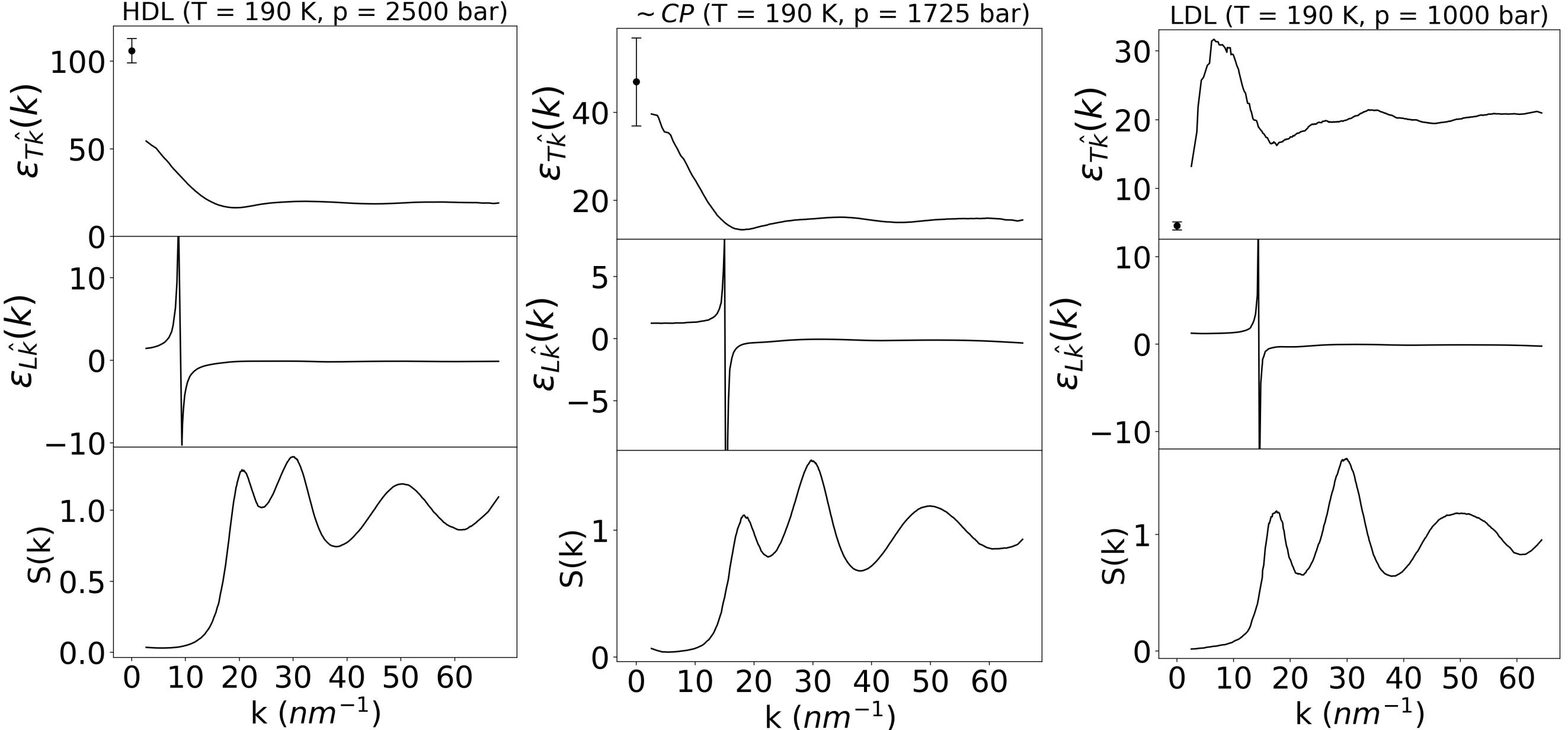
Figure 1: Non-local transverse (longitudinal) static dielectric functions, $\epsilon_{T(L)}(k)$ and static structure factor $S(k)$ in HDL, close to CP and in LDL. The black circle with the error bar, obtained by block averaging, in the upper graphs mark the value of $\epsilon_{0}$. The first peak in $S(k)$ corresponds to a minimum in $\epsilon_{T}(k)$, highlighting a possible link between the spatial arrangement of molecules’ center of mass and dipole orientation.

While there is never spontaneous magnetization in a finite system, the ferroelectric phase exhibits a nonzero $<P_{i}>$, as long as the box size $L$ of MD simulations exceeds the correlation length of the order parameter, as evident in Fig. 1. The brackets $<\ >$ denote ensemble average. Nevertheless, obtaining a full characterization of the polarization probability distribution is challenging because of spatial domains with varying polarization and orientation transitions. The $4th$ order cumulant of the polarization probability distribution, so-called Binder cumulant $U_{L}=1-\frac{1}{3}\frac{<P^{4}>}{<P^{2}>^{2}}$, has emerged as a powerful tool for discerning between paraelectric and ferroelectric phases [33, 34]. We derived $U_{L}$, $<\rho>$, the dielectric constant, $\epsilon_{0}$, and $K_{T}$ from MD simulations, as detailed in Section 1. It is $\epsilon_{0}=1+\chi$, where $\chi$ is the electric susceptibility. These quantities are shown in Fig. 2, supporting that the LLPT and the behavior at WL in supercooled water involves the dipolar degrees of freedom, as discussed below. (i) $U_{L}$ passes from about $4/9$, indicative of a paraelectric phase [34], to about $2/3$, indicative of a ferroelectric phase [34, 33], crossing from high $T$ both the WL (smooth transition) and the first order LLPT line (sharp transition). (ii) $<\rho>$ gradually decreases as it crosses the WL from high $T$, transitioning from typical values of HDL to LDL. The transitions of $<\rho>$ and $U_{L}$ co-occur. The $\rho$-transition expected when crossing the first-order LLPT line is obscured by the $<\rho>$-variation with $T$ at those p’s. (iii) Crossing the WL or the LLPT line from low $T$, $\epsilon_{0}$ increases to reach its maximum along the two lines. (iv) $K_{T}$ exhibits a maximum along the WL and the first-order LLPT line. Along the WL, the maximum value of $K_{T}$ increases as it approaches $\bar{p}_{c}$, where it diverges. Notably, unlike $K_{T}$, the peak value of $\epsilon_{0}$ remains almost unchanged along the WL and at CP. This evidences that, though coupled, $P$ and $\rho$ differently contribute to the free energy.

To characterize the local spatial distribution of masses and dipoles, Extended Data Fig. 1 shows the wavevector (k)-dependent transverse and longitudinal to k static dielectric functions, respectively $\epsilon_{T\hat{k}}(k)$ and $\epsilon_{L\hat{k}}(k)$, and the static structure factor, $S(k)$, in the HDL, LDL and close to CP. $\textbf{k}=k\hat{k}$ is the Fourier conjugate variable of the space variable r. Averages have been taken over different directions of k, as for all the quantities introduced in the following. Details are in Sec. 1. Extended Data Fig. 1 reveals divergences followed by negative $\epsilon_{L}$ values, akin to overscreening phenomena [39, 37]. Interestingly, in Ref. [40] water’s overscreening was attributed to $\rho$-$P$ fluctuations coupling.

0.2 A classical DFT for the ferroelectric LLPT

In one-component polar liquid, composed of non-polarizable molecules, the number density of particles at the point r having the unit vector $\hat{d}$ as dipole orientation is

$$\tilde{\rho}(\textbf{r},\hat{d})=\sum_{i=1}^{N}\delta(\hat{d}-\hat{d}_{i})\delta(\textbf{r}-\textbf{r}_{i})=\rho(\textbf{r})\zeta(\Omega,\textbf{r}),$$ (1)

where $\textbf{r}_{i}$ and $\hat{d}_{i}$ are respectively the center of mass position vector and dipole orientation of the $i$-th particle. $\rho(\textbf{r})$ and $\zeta(\textbf{r},\Omega)$ are respectively the particle number density without specified dipole orientation and the probability distribution of dipole orientation at point r. $\Omega$ is the solid angle element. To parameterize the Helmholtz free energy in terms of $\tilde{\rho}(\textbf{r})$, we decompose it into two parts: $F_{0}$, the free energy of a reference system devoid of dipole interaction, and the perturbative term $\mathcal{F}$, which incorporates dipole interaction. The structure of most liquids, especially at high density, is indeed primarily influenced by short-range hard-core pair interaction [35]. The perturbative effect will be treated via mean-field approximation, excluding from $\mathcal{F}$ contributions of $\tilde{\rho}(\textbf{r})$ correlations [35]. Assumption of spatial homogeneity fixes $\tilde{\rho}(\textbf{r})=\tilde{\rho}$. To facilitate comparison with MD simulations, the NpT ensemble [35] is used. The Gibbs free energy derived from the DFT, with detailed derivation in Sec. 1, is

$$G=\gamma_{0}(\bar{V})+\frac{a}{2}(T-T_{c})P^{2}+\frac{B}{4}P^{4}+\frac{B^{\prime}}{6}P^{6}+\frac{M}{2}\Delta V^{2}-p\beta\Delta VP^{2}+p\Delta V-\textbf{E}\cdot\textbf{P},$$ (2)

where $a$, $B$, $B^{\prime}$, $M$, and $\beta$ are positive constants, $\bar{V}$ is the equilibrium volume of the reference system, $\gamma_{0}$ is its Gibbs free energy, and $\Delta V$ is the difference between the system’s equilibrium volume ($V_{eq}$) and $\bar{V}$. The potential in Eq. 2 belongs to the class of potentials leading to tricritical points [27, 36], mirroring those of ferroelastic or magnetoelastic crystals [26, 27], where the deformation tensor replaces $p$.

The equilibrium values of P and $\Delta V$, $\textbf{P}{eq}$ and $\Delta V{eq}$, are determined through a variational principle,

$$\left.\frac{\partial G}{\partial\textbf{P}}\right|_{\textbf{P}=\textbf{P}_{eq}}=a(T-T_{c})\textbf{P}_{eq}+B\textbf{P}_{eq}^{3}+B^{\prime}\textbf{P}_{eq}^{5}-2p\beta\textbf{P}_{eq}\Delta V_{eq}-\textbf{E}=0;$$ (3)

$$\left.\frac{\partial G}{\partial\Delta V}\right|_{\Delta V=\Delta V_{eq}}=M\Delta V_{eq}-p\beta P_{eq}^{2}+p=0.$$ (4)

It follows

$$\Delta V_{eq}=-\frac{p}{M}(1-\beta P_{eq}^{2}).$$ (5)

The first term in Eq. 5 represents the liquid’s response to applied $p$, leading to compression, indicated by a negative contribution to $\Delta V_{eq}$. The second term shows that at a given $p$, $V_{eq}=\bar{V}+\Delta V_{eq}$ is larger when $P_{eq}\neq 0$ than when $P_{eq}=0$. Consequently, a ferroelectric phase exhibits lower density than a paraelectric phase. Eq. 5 formalizes the presence of a ferroelectric LDL phase and a paraelectric HDL. We are interested in the possible appearance of spontaneous polarization for $\textbf{E}=0$. The $P$-$\rho$ phase diagram in the ($p$, $T$) plane associated to Eq. 2 is obtained by analyzing the stability of solutions, Eqs. 3 and 4, set by the conditions $\chi,K_{T}>0$. See Section 1 and Supplementary Note II for detailed discussions. A schematic representation is shown in Fig. 3, with comments below.

1. Ferroelectric (first-order) LLPT. For constant $p>\bar{p}_{c}$ at $T=\hat{T}_{c}(p)$ a first-order ferroelectric LLPT is predicted. The following points support evidence for the first-order nature. (i) By lowering $T$ until $\hat{T}c$, $P$ switches abruptly from $P{eq}=0$ to $P_{eq}\neq 0$ (see Tab. 1 in Sec. 1), and the volume ($V$) shifts consequently from $V_{eq}=\bar{V}-\frac{p}{M}$ to $V_{eq}=\bar{V}-\frac{p}{M}(1-\beta P^{2}_{eq})$. (ii) There exists a $T$-range above and below $\hat{T}_{c}$ where the ferroelectric LDL and the paraelectric HDL, respectively, are metastable. (iii) Along the curve $T=\hat{T}_{c}(p)$ the two phases are both stable and coexist. (iv) At $T=\hat{T}_{c}(p)$, neither the $\chi$ nor $K_{T}$ diverges, but both reach a local maximum. (v) At $(\bar{T}_{c},\bar{p}_{c})$, the end point of the first-order phase transition, the $P$- and $V$-difference between the two phases goes to zero, while $\chi$ and $K_{T}$ diverge. Comparing with MD simulations in Sec. 0.1 identifies $T=\hat{T}_{c}(p)$ as the first-order LLPT curve.

   

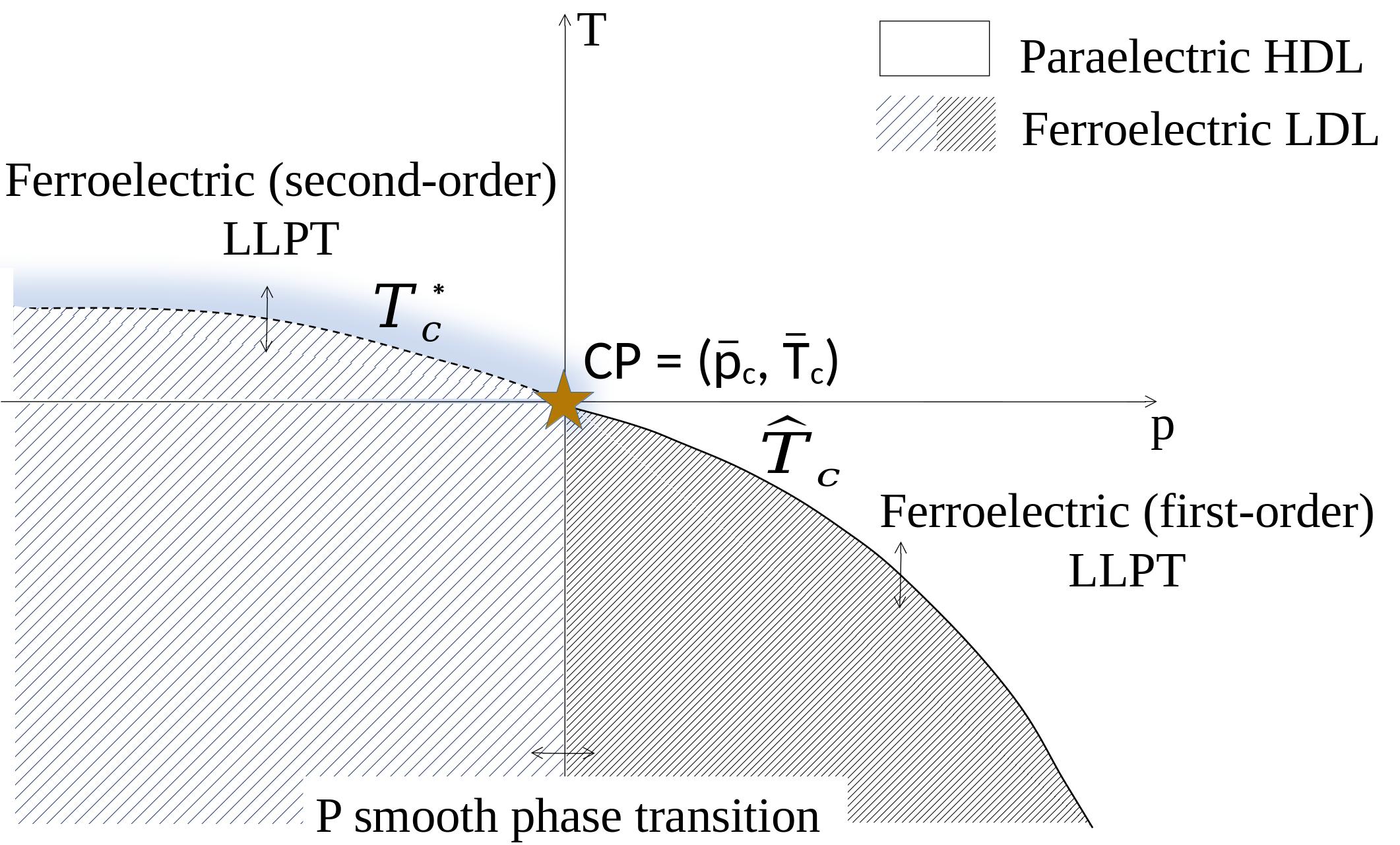
   Figure 3: Pictorial representation of the $P-\rho$ phase diagram of the polar liquid in the $($p,T$)$ plane obtained from DFT in mean field approximation. The critical point $CP=(\bar{p}_{c},\bar{T}_{c})$ is marked by a star. For $p<\bar{p}_{c}$ a first-order LLPT is predicted at $T=\hat{T}_{c}(p)$, represented by a full black line. For $p>\bar{p}_{c}$ a second-order ferroelectric LLPT is predicted at $T=T^{*}_{c}(p)$, marked by a black dashed line bordered by blue nuance. For $T<\bar{T}_{c}$ the theory predict a ferroelectric phase. A smooth transition in the $P$ value is predicted upon crossing the line $p=\bar{p}_{c}$. The two ferroelectric phases with different $P$ values are distinguished in the figure by varying degrees of line density within the texture.

2. Ferroelectric (second-order) continuous LLPT. At constant $p<\bar{p}_{c}$, the theory predicts a second-order ferroelectric phase transition at $T=T_{c}^{*}(p)$. The order parameter $P$ increases continuously from zero for $T<T_{c}^{*}$ (see Tab. 2 in Sec. 1). $V$ decreases continuously according to Eq. 5, indicating a simultaneous smooth $\rho$-transition. At $T=T_{c}^{*}(p)$, $\chi$ diverges. Relevantly, however, the theory predicts $K_{T}$ reaches a maximum rather than diverging at $T_{c}^{*}$. Along the curve $T=T_{c}^{*}(p)$, $K_{T}$ increases with increasing $p$ until it diverges at $\bar{p}_{c}$. Details are in Sec. 1. Though a finite scaling analysis is required to confirm $\epsilon_{0}$ divergence in MD simulations, the theory accurately predict the $K_{T}$, $U_{L}$ and $<\rho>$ trend at the WL. This consistency supports identifying the WL with the curve $T=T_{c}^{*}(p)$.

3. Smooth polarization magnitude phase transition. For $T<\bar{T}_{c}$, the system exhibits a ferroelectric phase. However, crossing the line $p=\bar{p}_{c}$ at a given $T<\bar{T}_{c}$ with increasing $p$, $P$ gradually increases and V decreases (refer to Tabs. 2 and 1 in Sec. 1). No singular behavior occurs in $\chi$ or $K_{T}$. Observing this transition in MD simulations is challenging due to the overlapping changes in $\Delta V$ and $\bar{V}$ when $p$ increases at fixed $T$. Also, measuring $P$ in MD simulations is demanding, as a non-zero average value is strictly only apparent in the macroscopic limit. Thus, we haven’t pursued this.

0.3 Ferroelectric order in LDL

MD simulations can uncover manifestations of the spontaneous breaking of the continuous symmetry group $O(3)$, characteristic of a ferroelectric phase, as outlined in the following. We opt for a reference system wherein one direction, $\hat{p}$, aligns with $\textbf{P}_{eq}$. (i) $\chi_{T\hat{p}}(k)$, the static susceptibility of the transverse to $\hat{p}$ polarization fluctuations, $\delta P_{T\hat{p}}$, diverges as $k^{-2}$ in the macroscopic limit $k\rightarrow 0$. (ii) So-called Goldstone modes emerge in $C_{T\hat{p}T\hat{p}}(k,t)$, the wavevector and time dependent correlation function of $\delta P_{T\hat{p}}$. Since polarization is conserved, the corresponding dispersion law approaches proportionality to $k^{2}$ in the small-$k$ limit. Detailed analysis is presented in Supplementary Note III in the framework of the Mori-Zwanzig memory function formalism [41]. (iii) Fluctuations in $\hat{p}$-longitudinal polarization, $\delta P_{L\hat{p}}$, can arise from fluctuations in $P$, $\delta P$, whose dynamics is empirically described by the Landau-Khalatnikov-Tani equation [42, 43]. This predicts collective modes, also known as Higgs-like modes [44], in the correlation function $C_{L\hat{p}L\hat{p}}(k,t)$ of $\delta P_{L\hat{p}}$, exhibiting propagating behavior with a linear dispersion relation at moderately small $k$ values [42], changing to constant as $k\rightarrow 0$. Goldstone-like and Higgs-like modes can coexists [44]. Coupling between $\delta P_{T\hat{p}}$ and $\delta P_{L\hat{p}}$ can arise from the constant-modulus principle [36], establishing that fluctuations in Gibbs free energy to lowest order in $\delta P_{T\hat{p}}$ satisfy the condition $\delta P^{2}=2P_{eq}\delta P_{L\hat{p}}+\delta P_{T\hat{p}}^{2}=0$ [36]. It implies that (i) the static $\hat{p}$-longitudinal polarization susceptibility, $\chi_{L\hat{p}}$, diverges for $k\rightarrow 0$ as $k^{-1}$ [36]. (ii) Propagating Goldstone-like modes persists in $C_{T\hat{p}T\hat{p}}(k,t)$ but they are not induced in $C_{L\hat{p}L\hat{p}}(k,t)$. (iii) Spontaneous fluctuations in $P$ generate a collective mode both in $C_{L\hat{p}L\hat{p}}(k,t)$ and $C_{T\hat{p}T\hat{p}}(k,t)$, with the same dispersion relation. Further details are provided in Supplementary Note III. Finally, if a collective mode emerges in $C_{L\hat{p}L\hat{p}}(r,t)$, it corresponds to a mode in the density correlation function $C_{\rho\rho}(k,t)$ due to the coupling between $P$ and $\rho$, see Eq. 2.

The predictions above find confirmation in the analysis of MD simulations. Specifically, (i) both $\chi_{T\hat{p}}$ and $\chi_{L\hat{p}}$ in Panel a of Fig. 4 show a significant enhancement for $k\rightarrow 0$, approximately following $k^{-2}$ and $k^{-1}$ law, respectively. (ii) $\delta P_{L\hat{p}}$, $\delta P_{T\hat{p}}^{2}$ and $\delta\rho$ correlate, as emphasized in Panel b of Fig. 4. (iii) A propagating mode in $C_{T\hat{p}T\hat{p}}(k,t)$, $C_{L\hat{p}L\hat{p}}(k,t)$ and $C_{\rho\rho}(k,t)$, reflecting in a their oscillatory behavior, is observed. Oscillations are significantly reduced in $C_{PP}(k,t)$, showing that the constant-modulus principle is approximately satisfied. The presence of a propagating mode in both $C_{T\hat{p}T\hat{p}}(k,t)$ and $C_{L\hat{p}L\hat{p}}(k,t)$, along with a preliminary assessment of the dispersion relation indicating linearity in $k$, suggests that the observed propagating mode originates from fluctuations in $P$. As shown in Supplementary Note IV, where different points of the ($T$, $p$) plane are analyzed, in HDL propagating modes vanish, and correlation functions decay to zero on a timescale much shorter than $\mu s$.

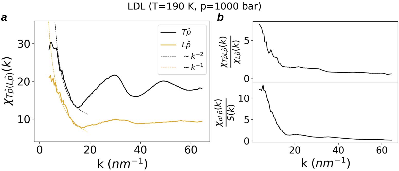
Figure 4: a: Static susceptibilities $\chi_{T\hat{p}(L\hat{p})}(k)$, in LDL as a function of $k$. Both $\chi_{T\hat{p}}$ and $\chi_{L\hat{p}}$ exhibit significant enhancement as $k\rightarrow 0$, roughly following $k^{-2}$ and $k^{-1}$, respectively, as indicated by the dashed lines, consistent with predictions for a ferroelectric phase with spontaneous breaking of $O(3)$ symmetry group. b, The upper graph illustrates the static correlation between $\delta P_{L\hat{p}}$ and $\delta P_{T\hat{p}}^{2}$, $\chi_{T\hat{p}L\hat{p}}(\textbf{k})\propto|<\hat{p}\cdot\delta\textbf{P}_{L\hat{p}}^{*}(\textbf{k})\delta\textbf{P}_{T\hat{p}}(\textbf{k})^{2}>|$, averaged on $\hat{k}$, over $\chi_{L\hat{p}}(k)$ in LDL. The lower graph depicts the static correlation between $\delta\rho$ and $\delta P_{L\hat{p}}$, $\chi_{\rho L\hat{p}}(\textbf{k})\propto|<\rho^{*}(\textbf{k})\hat{p}\cdot\delta\textbf{P}_{L\hat{p}}(\textbf{k})>|$, averaged on $\hat{k}$, over $S(k)$ in LDL. A correlation between $\delta P_{L\hat{p}}$, $\delta P_{T\hat{p}}^{2}$ and $\delta\rho$ emerges, in particular at moderately small $k$s.

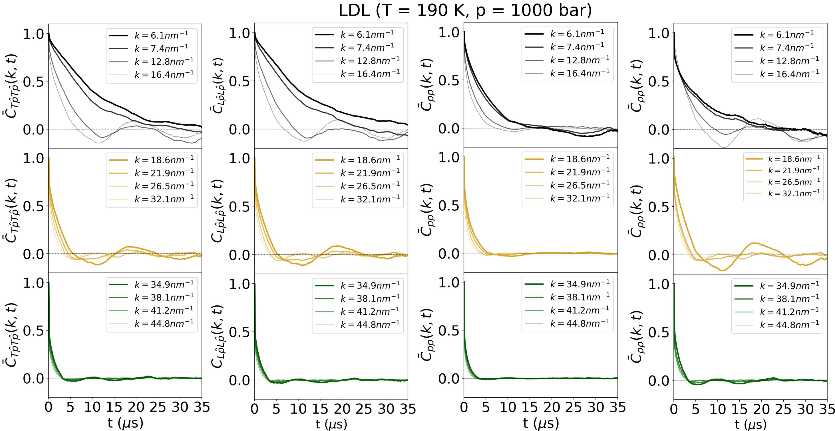
Figure 5: Correlation functions, from left to right, $C_{T\hat{p}T\hat{p}}(k,t)$, $C_{L\hat{p}L\hat{p}}(k,t)$, $C_{PP}(k,t)$, $C_{\rho\rho}(k,t)$ at different $k$ values. All quantities have been normalized to their value at $t=0$, being $\bar{C}(k,t)=C(k,t)/C(k,0)$. Oscillatory behavior in $C_{L\hat{p}L\hat{p}}(k,t)$ and $C_{T\hat{p}T\hat{p}}(k,t)$ indicates the presence of a collective propagating mode, consistent with the existence of a ferroelectric phase leading to the spontaneous breaking of the $O(3)$ symmetry group. Oscillations are significantly reduced in $C_{PP}(k,t)$, suggesting that the constant modulus principle is approximately satisfied. The observation of a propagating collective mode in $C_{\rho\rho}(k,t)$ highlights an existing correlation between $P$ and $\rho$, as also emphasized in Panel b of Fig. 4.

0.4 Conclusions

The analysis of MD simulations from Ref. [4] alongside the construction of a classical DFT for polar liquids under mean-field approximation highlighted the role of dipolar degrees of freedom in the first-order LLPT and the behavior around the WL. Consistently with a second-order ferroelectric phase transition, the theory predicts a $\chi$ divergence at the WL. A finite-size scaling analysis is needed to confirm the divergence of $\chi$ in MD simulations. The mean-field treatment proposed here is not expected, however, to describe the critical exponents properly [17]. Remarkably, it was recently shown that anharmonicity in the Gibbs free energy, akin to Eq. 2, in the ferroelectric phase can lead to $P$ fluctuations with a non-zero ensemble average. These fluctuations could reduce $P$ and, consequently, suppress the divergence of $\chi$. Another hypothesis, which might explain the possible lack of $\chi$ divergence, is the occurrence of an improper ferroelectric phase transition [26], where the order parameter has multiple components, and the low-$T$ phase exhibits pyroelectric properties. An interesting choice for the order parameter components could be classifiers of topological order degree, introduced in Ref. [13]. The lower entanglement of the hydrogen-bond network in LDL compared to HDL [13] could favor dipole alignment. Ref. [45] suggested a two-order-parameter description for supercooled liquids.

Our study suggests that experimental validation of the LLPT in water can involve analyzing dielectric properties. It can be, furthermore, investigated whether an electric field can induce LLPT in water [46], and its relationship with the $p$ and $T$-induced LLPT analyzed here.

Since Pauling in 1935, attributing residual entropy in hexagonal ice to configurational proton disorder [48], the concept of frustration and disorder in dipole-lattice models of ice [49] was introduced. It would be intriguing to explore whether positional and dipolar orders compete. A phase featuring dipolar order and structural disorder in LDL might correspond to one with structural order and dipolar disorder in hexagonal ice. Finally, An alternative perspective worth considering is a glass transition in the dipolar degrees of freedom, leading to the LDL phase. This aligns with observations that $U_{L}$ in systems with quenched spin disorder is comparable to that with ordered spins [47]. Nevertheless, existence of residual order must be considered, given the non-zero value of $P_{i}$. If a maximum rather than a divergence were confirmed in $\chi$, it would further bolster this idea. The observed propagating collective modes in the polarization correlation functions may be linked to the breakdown of replica symmetry, possibly accompanying the dipole glass transition [50].

1 Methods

1.1 MD simulations of TIP4P/ice water

The MD simulations analyzed are the same of Ref. [4], where further details can be found. The MD simulations, performed with GROMACS, employed the classical TIP4P/Ice water model [32] with $N=1000$ molecules in NpT ensemble, using a time-step of $2\ fs$. This model features rigid molecule geometry with a dipole moment of $d=2.426\ D$. Nosé–Hoover thermostat and the isotropic Parrinello–Rahman barostat were used with characteristic time scale around respectively 10 ps and 20 ps. Electrostatic interactions were calculated by the particle-mesh Ewald method with a cutoff distance of $0.9$ nm. Van der Waals interactions has the same cutoff.

1.2 Analysis of MD simulations

Electric susceptibility and isothermal compressibility are respectively obtained from MD simulations as follows:

$$\chi=\frac{<P^{2}>-<P>^{2}}{3e_{0}<V>K_{B}T};$$ (6)

$$K_{T}=\frac{<V^{2}>-<V>^{2}}{<V>K_{B}T}.$$ (7)

$K_{B}$ is the Boltzmann constant and $e_{0}$ the vacuum permittivity. The ensemble average is obtained from MD simulations by making use of the ergodicity hypothesis, thus $<O>=\bar{t}^{-1}\sum_{t=1}^{\bar{t}}O(t)$, where $O$ is a generic observable, $t=n\Delta t$ with $n\in\mathbb{N}$, $\Delta t$ is a time step and $\bar{t}$ is the time-length of MD simulations. In the present case $\Delta t\sim 8\ 10^{-2}ps$ for all the probed points in the ($p$, $T$) plane. The value of $U_{L}$ in a paraelectric and ferroelectric phase are established following the observations below. In the paraelectric phase, stochastic Gaussian fluctuations centered around a zero $P$ value result in $U_{L}\rightarrow\frac{2(n-1)}{3n}$ as $L\rightarrow\infty$ for $O(n)$ model [34]. In the present case with $n=3$, $U_{L}\rightarrow\frac{4}{9}$. In the ferroelectric phase, where a non-zero $P$ set in, $U_{L}\rightarrow\frac{2}{3}$, $\forall n$ [34, 33].

The static structure factor is obtained as

$$S(\textbf{k})=<\delta\rho^{*}(\textbf{k})\delta\rho(\textbf{k})>,$$ (8)

where the $\rho$ fluctuations $\delta\rho(\textbf{k})=\frac{1}{\sqrt{N}}\sum_{i=1}^{N}e^{i\textbf{k}\cdot\textbf{r}_{i}}$. The components of k are derived from the expression $k_{i}=\frac{2\pi}{L}$, with $i=x,y,z$. $L$ is the time-averaged simulation box size. Using instantaneous values of $L$ does not induce any substantial change. It is $L\sim 3.2$ nm, thus $\Delta k_{i}=2\pi/L\sim 1.9$ nm^-1. Averages have been taken over different directions of k. Further averaging within a $\pm\Delta k$ with $\Delta k=1.8\ nm^{-1}$ k-interval centered around a specific $k$ has been conducted to enhance the visual examination without altering the overall trends of the quantities represented. The same averaging procedure over k-directions and $\Delta k$ has been applied to all the static and dynamic correlation functions. Since $S(k\rightarrow 0)=\rho K_{B}TK_{T}$, at CP $S(k\rightarrow 0)$ should diverge. In Extended Data Fig. 1 it is observed a gradual rise in $S(k)$ for small $k$ values at the thermodynamic point close to CP. A more pronounced increase, indicative of a divergence as $k\rightarrow 0$, is observed at a $k$-scale smaller than what is attainable in the current MD simulations with $N=1000$ [4].

The k-dependent static susceptibilities, transverse and longitudinal to k, are obtained from MD simulations as:

$$\chi_{T\hat{k}(L\hat{k})}(\textbf{k})=\frac{<\delta\textbf{P}_{T\hat{k}(L\hat{k})}^{*}(\textbf{k})\cdot\delta\textbf{P}_{T\hat{k}(L\hat{k})}(\textbf{k})>}{e_{0}<V>K_{B}T},$$ (9)

where the symbol $"\cdot"$ represents the scalar product. $\delta\textbf{P}_{T\hat{k}}(\textbf{k})=\hat{k}\times\delta\textbf{P}(\textbf{k})$, $\delta\textbf{P}_{L\hat{k}}(\textbf{k})=\frac{\delta\rho_{c}}{k}\ \hat{k}$, with $\delta\textbf{P}(\textbf{k})=\sum_{i=1}^{N}e^{i\textbf{k}\cdot\textbf{r}_{i}}(\textbf{d}_{i}-<\textbf{d}_{i}>)$ and $\delta\rho_{c}=\sum_{i=1}^{N}\sum_{\alpha}e^{i\textbf{k}\cdot(\textbf{r}_{i}+\delta\textbf{r}_{i\alpha})}z_{\alpha}e$. The vectors $\textbf{d}_{i}=d\ \hat{d}_{i}$ and $\textbf{r}_{i}$ are respectively the dipole and vector position of the center of mass of the $i$-th particle, $\delta\textbf{r}_{i\alpha}$ are spatial coordinates of molecular sites, $z_{\alpha}$ is the partial charge of site $\alpha$, and $e$ the elementary charge. We prefer the definition of $\delta\textbf{P}_{L\hat{k}}(\textbf{k})$ provided above, rather than $\delta\textbf{P}_{L\hat{k}}(\textbf{k})=\hat{k}\cdot\delta\textbf{P}(\textbf{k})\ \hat{k}$, because it has been shown [37] that the latter yields less accurate results at finite $k$ due to the approximation of extended molecular dipoles as point dipoles. The symbol ^∗ states for complex conjugate. As for the definitions given above, $\chi_{T\hat{k}(L\hat{k})}(\textbf{k})$ are related to the space-dependent $P$ fluctuations. $\epsilon_{T(L)}(\textbf{k})$ are obtained from $\chi_{T\hat{k}(L\hat{k})}(\textbf{k})$ as follows: $\epsilon_{T}(\textbf{k})=1+\chi_{T\hat{k}}(\textbf{k})$ and $\epsilon_{L}(\textbf{k})=1/(1-\chi_{L\hat{k}}(\textbf{k}))$ [37, 38]. For $k\neq 0$, $\epsilon_{T}(k)$ holds only the physical meaning of a static correlation function, preserving $\epsilon_{T}(k)-1$ the quality of a response function only in the limit $k\rightarrow 0$, while $\chi_{L}(k)=1/(1-\epsilon_{L}(k))$ is a static response function [38]. This implies that for a thermodynamically stable system, $\epsilon_{L}(k)\geq 1$ or $\epsilon_{L}(k)<0$ [38, 37]. Additionally, a divergence occurs when $\epsilon_{L}=1$ as the one observed in Extended Data Fig. 1. Another divergence has been noted at higher $k$ values in ambient water conditions [37], ensuring the correct physical limit $\lim_{k\rightarrow\infty}\epsilon_{L}(k)=1$ [37].

The non-local static susceptibilities $\chi_{T\hat{p}(L\hat{p})}(\textbf{k})$ are obtained from the following expression

$$\chi_{T\hat{p}(L\hat{p})}(\textbf{k})=\frac{<\delta\textbf{P}_{T\hat{p}(L\hat{p})}^{*}(\textbf{k})\cdot\delta\textbf{P}_{T\hat{p}(L\hat{p})}(\textbf{k})>}{e_{0}<V>K_{B}T},$$ (10)

where $\delta\textbf{P}_{T\hat{p}}(\textbf{k})=\hat{p}\times\delta\bar{\textbf{P}}(\textbf{k})$, $\delta\textbf{P}_{L\hat{p}}(\textbf{k})=\hat{p}\cdot\delta\bar{\textbf{P}}(\textbf{k})\ \hat{p}$, $\delta\bar{\textbf{P}}(\textbf{k})=\sum_{i=1}^{N}e^{i\textbf{k}\cdot\textbf{r}_{i}}(\textbf{d}_{i}-\bar{\textbf{d}})$. Strictly, it holds that $\bar{\textbf{d}}=\textbf{P}{eq}/N$ and $\hat{p}=\textbf{P}{eq}/P_{eq}$. In finite-size systems we approximate $\textbf{P}_{eq}$ as $<\textbf{P}>$. Due to the assumption $\textbf{P}_{eq}=<\textbf{P}>$ , the value of $\chi_{T\hat{p}}(\textbf{k}=0)$ and $\chi_{T\hat{p}}(\textbf{k}=0)$ cannot be obtained from MD simulations. Instead, we have $\delta\bar{\textbf{P}}(k=0)=\delta\textbf{P}(k=0)$ defined above. Consequently, $\chi_{T\hat{p}}(\textbf{k}=0)+\chi_{L\hat{p}}(\textbf{k}=0)=\chi$. The electric susceptibility $\chi$ remains finite in the ferroelectric phase. The static correlation functions $\chi_{T\hat{p}L\hat{p}}(\textbf{k})$, $\chi_{\rho L\hat{p}}(\textbf{k})$, computed to unveil static correlation between $\delta\rho$, $\delta\textbf{P}_{L\hat{p}}$, $\delta\textbf{P}^{2}_{T\hat{p}}$ are obtained from MD simulations as:

$$\chi_{T\hat{p}L\hat{p}}(\textbf{k})=\frac{|<\hat{p}\cdot\delta\textbf{P}_{L\hat{p}}^{*}(\textbf{k})\delta\textbf{P}_{T\hat{p}}(\textbf{k})^{2}>|}{[e_{0}<V>K_{B}T]^{3/2}},$$ (11)

$$\chi_{\rho L\hat{p}}(\textbf{k})=\frac{|<\rho^{*}(\textbf{k})\hat{p}\cdot\delta\textbf{P}_{L\hat{p}}(\textbf{k})>|}{[e_{0}<V>K_{B}T]^{1/2}}.$$ (12)

The dynamic correlation functions are obtained from the expressions

$$C_{T\hat{p}T\hat{p}(L\hat{p}L\hat{p})}(\textbf{k},t)=<\delta\textbf{P}^{*}_{T\hat{p}(L\hat{p})}(\textbf{k},0)\cdot\delta\textbf{P}_{T\hat{p}(L\hat{p})}(\textbf{k},t)>,$$ (13)

$$C_{PP}(\textbf{k},t)=<\delta\textbf{P}^{*}(\textbf{k},0)\cdot\delta\textbf{P}(\textbf{k},t)>,$$ (14)

$$C_{\rho\rho}(\textbf{k},t)=<\delta\rho^{*}(\textbf{k},0)\delta\rho(\textbf{k},t)>.$$ (15)

The correlation functions are computed with a time interval $\Delta t\sim 8\ 10^{-2}\mu s$.

1.3 Setting the density functional theory of ferroelectric LLPT

The free energy of a reference system without dipole interaction, $F_{0}$, and the extra free energy term, $\mathcal{F}$, accounting for dipole interaction in mean field approximation, i.e. neglecting contribution of $\tilde{\rho}(\textbf{r},\hat{d})$ correlations [35] are, respectively,

$$F_{0}=\phi_{0}+T\int d\textbf{r}\ d\Omega\ \rho(\textbf{r})\zeta(\textbf{r},\Omega)\ln[4\pi\zeta(\textbf{r},\Omega)];$$ (16)

$$\mathcal{F}=\frac{1}{2}\int\int d\textbf{r}\ d\Omega\ d\textbf{r}^{\prime}\ d\Omega^{\prime}\ \rho(\textbf{r})\zeta(\textbf{r},\Omega)w_{p}(\textbf{r},\textbf{r}^{\prime},\Omega,\Omega^{\prime})\rho(\textbf{r}^{\prime})\zeta(\textbf{r}^{\prime},\Omega^{\prime}),$$ (17)

where $d\Omega$ is the infinitesimal element of solid angle and the integral is extended to the whole solid angle. To streamline the notation we assume here $K_{B}=1$. $\phi_{0}$ arises from the internal energy of the reference system along with the entropy term of the positional degrees of freedom. The second term on the right-hand side of Eq. 16 represents the dipole orientational entropy [30]. Though non-interacting, the dipoles are still present in the reference system. The dipole interaction in Eq. 17 is

$$w_{p}(\textbf{r},\textbf{r}^{\prime},\Omega,\Omega^{\prime})=-\frac{d^{2}}{R^{3}}[3(\hat{d}(\textbf{r})\cdot\hat{R})(\hat{d}(\textbf{r}^{\prime})\cdot\hat{R})-\hat{d}(\textbf{r})\cdot\hat{d}(\textbf{r}^{\prime})],$$ (18)

where $\textbf{R}=R\hat{R}=\textbf{r}-\textbf{r}^{\prime}$, $\hat{d}(\textbf{r})$ is a unit vector at the point r. Spatial homogeneity, leading to $\tilde{\rho}(\textbf{r},\hat{d})=\tilde{\rho,\hat{d}}$, is assumed. To solve the mean-field DFT model, specifically, to find the equilibrium value of $\tilde{\rho}$ through a variational principle, we use the following ansatz for the dipole orientation distribution

$$\zeta(\Omega,\textbf{r})=\zeta(\Omega)=\frac{1+\boldsymbol{\delta}\hat{d}}{4\pi}.$$ (19)

$\boldsymbol{\delta}=\delta\hat{\delta}$ satisfies $\int d\Omega\ \hat{d}(\Omega)\zeta(\Omega)=\boldsymbol{\delta}$. If $\delta\neq 0$, the polar liquid show a non-zero total polarization $\textbf{P}=d\int d\textbf{r}\rho(\textbf{r})\int\hat{d}(\Omega)d\Omega\zeta(\Omega)=dN\boldsymbol{\delta}$, otherwise the system is isotropic and $\zeta(\Omega)$ is the uniform distribution. $\delta$, is assumed to be small, i.e. small deviations from system’s isotropy are considered. The $\delta$-Taylor expansion around zero of $F_{0}$ and $\mathcal{F}$ in Eq. 16 and Eq. 17, respectively, yields:

$$F_{0}=\phi_{0}(\rho)+TN[A\delta^{2}+B\delta^{4}+B^{\prime}\delta^{6}];$$ (20)

$$\mathcal{F}=-N\beta(\rho)\rho\delta^{2}.$$ (21)

$A,B,B^{\prime}$, which are independent of both $T$ and $p$ as $\zeta(\Omega)$ is assumed to be so, are positive constants. We expanded $F_{0}$ up to sixth order in $P$ since lower-order coefficients can be zero. To obtain Eq. 21, due to positional disorder, a uniform distribution of the angle between $\hat{\delta}$ and $\hat{R}$ is assumed. This leads to a negative integral in Eq. 17, thus setting $\beta(\rho)>0$. There is no Taylor series truncation because given the functional form of the dipolar interaction higher order terms in $\delta$-powers are zero. Implicitly, $R\neq 0$ due to the repulsive short-range term in the reference system’s interaction potential, ensuring the integral over $R$ to be finite. $\rho$ slightly deviates from the reference system’s density, $\bar{\rho}$, because the dipole interaction is a slight perturbation to the pair interaction potential of the reference system. Consequently, $\phi(\rho)$ and $\mathcal{F}(\rho)$ in Eq. 20 and Eq. 21, respectively, can be given by a Taylor series in $\rho$. The $\rho$-Taylor expansion around $\bar{\rho}$ of $F_{0}$ and $\mathcal{F}$, truncated to lowest order, leads to

$$F_{0}=N\phi_{0}(\bar{\rho})+MN\Delta\rho^{2}+TN[A\delta^{2}+B\delta^{4}+B^{\prime}\delta^{6}];$$ (22)

$$\mathcal{F}=\mathcal{F}(\bar{\rho})+\frac{\partial\mathcal{F}}{\partial\rho}|_{\bar{\rho}}\Delta\rho=-N\beta_{0}(\bar{\rho})\bar{\rho}\delta^{2}+N\beta_{1}(\bar{\rho})\bar{\rho}\delta^{2}\Delta\rho.$$ (23)

It is $\Delta\rho=\rho-\bar{\rho}$. Since $\bar{\rho}$ is the equilibrium density of the reference system, $\phi^{\prime}(\bar{\rho})=0$, and $M=\frac{1}{2N}\phi^{\prime\prime}(\bar{\rho})>0$. The single and double prime notation denotes, respectively, the first and second derivatives of $\phi$ in $\rho$. It is $\beta_{0}(\bar{\rho}),\beta_{1}(\bar{\rho})>0$. $\frac{\partial\mathcal{F}}{\partial\rho}|_{\bar{\rho}}>0$ because an increase in $\rho$, resulting in a $V$ decrease, leads to an increment of the integral in Eq. 17, given Eq. 19 and the assumption of a uniform angle distribution between $\hat{\delta}$ and $\hat{R}$ endorsed above. Finally, considering that $\boldsymbol{\delta}\propto\textbf{P}$,

$$F/N=\phi_{0}(\bar{\rho})+M\Delta\rho^{2}+[TA-\beta_{0}(\bar{\rho})\bar{\rho}]P^{2}+TBP^{4}+TB^{\prime}P^{6}]+\beta_{1}(\bar{\rho})P^{2}\Delta\rho.$$ (24)

The constants in Eq. 24 have been redefined, retaining, however, the same names as before. The thermodynamic potential in the NpT ensemble [35], we want to use here, is the Gibbs free energy $G=F_{0}+\mathcal{F}+pN/\rho$. $\rho$ changes are induced by $V$ variations, yielding $\bar{\rho}=N/\bar{V}$ and $\Delta\rho=-\bar{\rho}\Delta V/\bar{V}$. Considering that $\boldsymbol{\delta}$ is proportional to the total polarization P, and featuring an external electric field E conjugate to P, we obtain Eq. 2, which we write below for clarity,

$$G=\gamma_{0}(\bar{V})+\frac{a}{2}(T-T_{c})P^{2}+\frac{B}{4}P^{4}+\frac{B^{\prime}}{6}P^{6}+\frac{M}{2}\Delta V^{2}-p\beta\Delta VP^{2}+p\Delta V-\textbf{E}\cdot\textbf{P}.$$ (25)

The term $\gamma_{0}(\bar{V})$ includes the additive term $p\bar{V}$. In Eq. 25 it has been assumed that for a given $p$ it exists a value of $T\equiv T_{c}:T_{c}A-\beta_{0}\bar{\rho}(T_{c},p)=0$. We neglect the $p$ dependence of $T_{c}$ for sake of simplicity. Since at $T_{c}$ the coefficient in front of $P^{2}$ becomes zero, for $T$ near $T_{c}$ we neglect the $T$ dependence of all the other coefficients. The $p$ dependence of $M$ is also irrelevant to our aim. Consequently, $a$, $B$, $B^{\prime}$, and $M$ are positive constants. $\beta_{1}(\bar{\rho})$ in Eq. 24 still depends on $p$. For sake of simplicity we assume $\beta_{1}=\beta p$ with $\beta>0$. The factors like $1/2$ in front of $a$ have been introduced for convenience.

1.4 The variational principle solution for the mean field model

With the thermodynamic potential provided in Eq. 2, the equilibrium values of P and $\Delta V$, $\textbf{P}{eq}$ and $\Delta V{eq}$ respectively, are determined through the variational principle establishing that at equilibrium the thermodynamic potential must be minimized. $\textbf{P}{eq}$ and $\Delta V{eq}$, are obtained by solving Eqs. 3 and 4. Eq. 5 further outlines the link existing between $\textbf{P}{eq}$ and $\Delta V{eq}$. By inserting the value of $\Delta V_{eq}$ in Eq. 5 it is obtained

$$a(T-T_{c}+\frac{2\beta}{aM}p^{2})\textbf{P}_{eq}+(B-\frac{2\beta^{2}}{M}p^{2})\textbf{P}_{eq}^{3}+B^{\prime}\textbf{P}_{eq}^{5}-2\beta\textbf{P}_{eq}\Delta V_{eq}-\textbf{E}=0.$$ (26)

It is convenient to define

$$T_{c}^{*}(p)=T_{c}-2\frac{\beta}{aM}p^{2};$$ (27)

$$B^{*}(p)=B-\frac{2\beta^{2}}{M}p^{2}.$$ (28)

$T_{c}^{*}$ is the temperature at which the term proportional to $\textbf{P}_{eq}$ in Eq. 26 disappears. There exists a $p$ at which $B^{*}=0$, causing, instead, the term proportional to $\textbf{P}_{eq}^{3}$ to become zero in Eq. 26. We further define

$$\bar{p}_{c}:B^{*}(\bar{p}_{c})=0;$$ (29)

$$\bar{T}_{c}=T_{c}^{*}(\bar{p}_{c}).$$ (30)

The solutions of Eqs. 3 and 4 are stable if for $P=P_{eq}$ and $\Delta V=\Delta V_{eq}$, $\chi$ and $K_{T}$ are positive, i.e.

$$\chi=\frac{\partial\textbf{P}}{\partial\textbf{E}}|_{N,T,p}>0;\ \ K_{T}=-\frac{1}{V}\frac{\partial V}{\partial p}|_{N,T,\textbf{E}}>0.$$ (31)

We are interested to the possible appearance of spontaneous polarization, thus to solutions of Eqs. 3 and 4 for $\textbf{E}=0$. From Eqs. 3, 4 and 31, it is found

$$\chi=\frac{1}{a(T-T_{c}^{*})+3B^{*}\textbf{P}_{eq}^{2}+5B^{\prime}\textbf{P}_{eq}^{4}};\ \ \ \$$ (32)

$$K_{T}=\bar{K}_{T}+\Delta K_{T}=-\frac{1}{V}\frac{\partial\bar{V}}{\partial p}+\frac{1}{VM}\frac{a(T-T_{c}^{*})+3B^{*}\textbf{P}_{eq}^{2}+5B^{\prime}\textbf{P}_{eq}^{4}+4\frac{(\beta p)^{2}}{M}\textbf{P}_{eq}^{2}}{a(T-T_{c}^{*})+3B^{*}\textbf{P}_{eq}^{2}+5B^{\prime}\textbf{P}_{eq}^{4}}.$$

(33)

$\bar{K}_{T}$ and $\Delta\bar{K}_{T}$ are implicitly defined in Eq. 33. It is $\bar{K}_{T}>0$ because $\bar{V}$ is the $V$ of a stable state of the reference system. The equilibrium values of $P$, obtained by solving Eqs. 3 and 4, satisfying the stability conditions given by Eqs. 31, are reported in Tab. 1 and Tab. 2 for $p$ respectively larger and smaller than $\bar{p}_{c}$. The corresponding value of $\Delta V_{eq}$ can be obtained from Eq. 5. For $p>\bar{p}_{c}$ two stable solutions are found in the $T$ ranges specified in Tab. 1, one of which is metastable as deduced by calculating the thermodynamic potential for each solution. For $p<\bar{p}_{c}$ only one stable solution exists for both $T>T_{c}^{*}$ and $T<T_{c}^{*}$. At a given $T<\bar{T}_{c}$, the difference $\Delta P^{2}_{eq}=P^{2}_{eq}(p>\bar{p}_{c})-P^{2}{eq}(p<\bar{p}_{c})=\frac{B^{*}(p)}{2B^{\prime}}\neq 0$ unless $p=\bar{p}_{c}$, where $B^{*}=0$. The value of $\hat{T}_{c}(p)$ and $\bar{T}$ in Tab. 1 are

$$\hat{T}_{c}(p)=\frac{3}{16}\frac{{B^{*}(p)}^{2}}{aB^{\prime}}+T_{c}^{*}(p);$$ (34)

$$\bar{T}(p)=\frac{1}{4}\frac{{B^{*}(p)}^{2}}{aB^{\prime}}+T_{c}^{*}(p)$$ (35)

Further details are reported in the Supplementary Note I. The behavior of $K_{T}$ at and along the WL is obtained in the following. For $T\rightarrow{T_{c}^{*}}^{-}$, $P_{eq}^{2}\simeq\frac{a(T_{c}^{*}-T)}{B^{*}}$. From Eq. 33 it is

$$\Delta K_{T}|_{T\rightarrow{T_{c}^{*}}^{-}}=\frac{1}{VM}[1+\frac{4(\beta p)^{2}}{MB^{*}}\frac{1}{2+5\frac{aB^{\prime}}{B^{*}}(T_{c}^{*}-T)}].$$ (36)

As $T\rightarrow{T_{c}^{*}}^{+}$, from Eq. 33, we find $\Delta K_{T}=\frac{1}{VM}$, indicating an increase in $\Delta K_{T}$ due to the $V$ reduction caused by the temperature decrease. As $T\rightarrow{T_{c}^{*}}^{-}$, according to Eq. 36, $\Delta K_{T}$ also increases. Furthermore, Eq. 36 demonstrates that $\Delta K_{T}$ remains finite at $T_{c}^{*}$, where it reaches a maximum, as inferred from the observations above. Along the curve $T=T_{c}^{*}$, where $\Delta K_{T}$ is maximum, $\Delta K_{T}|_{T=T_{c}^{*}}=\frac{1}{VM}[1+\frac{4(\beta p)^{2}}{MB^{*}}]$. Considering the definition of $B^{*}$ in Eq. 28, $\Delta K_{T}|_{T=T_{c}^{*}}$ increases by moving along the curve $T=T_{c}^{*}$ by increasing $p$ until it diverges at $\bar{p}_{c}$. We can assume $\bar{K}_{T}$ to be constant in a sufficiently small neighborhood of $T_{c}^{*}$.

Table 1: Equilibrium values of $P$ for the thermodynamic potential given by Eq. 2 for $p>\bar{p}_{c}$. A dash indicates that the solution is not stable. The value of $\hat{T}_{c}$ and $\bar{T}$ is reported in Eq. 34 and Eq. 35, respectively.

$p>\bar{p}_{c}$	$P^{2}_{eq}=$	$P^{2}_{eq}=$
	$-\frac{B^{*}}{2B^{\prime}}+\frac{1}{2B^{\prime}}\sqrt{{B^{*}}^{2}-4a(T-T_{c}^{*})B^{\prime}}$	0
$T<T_{c}^{*}$	stable	-
$T_{c}^{*}<T<\hat{T}_{c}$	stable	metastable
$\hat{T}_{c}<T<\bar{T}$	metastable	stable
$T>\bar{T}$	-	stable

Table 2: Equilibrium values of $P$ for the thermodynamic potential given by Eq. 2 for $p<\bar{p}_{c}$. A dash indicates that the solution is not stable.

$p<\bar{p}_{c}$	$P^{2}_{eq}=$	$P^{2}_{eq}=$
	$\frac{B^{*}}{2B^{\prime}}+\frac{1}{2B^{\prime}}\sqrt{{B^{*}}^{2}-4a(T-T_{c}^{*})B^{\prime}}$	0
$T>T_{c}^{*}$	-	stable
$T<T_{c}^{*}$	stable	-

Author Contribution

M. G. I. conceived the idea that ferroelectricity can play a role in the liquid-liquid phase transition. M. G. I., G. P., J. R. discussed, designed and projected research. M. G. I. performed MD simulations data analysis, interpretation and theoretical developments. M. G. I., G. P., J. R. discussed the results. M. G. I. wrote the paper. G. P., J. R. revised the paper.

2 Extended Data

References

- [1] Angell, C. A. in Water: A Comprehensive Treatise (ed. F. Franks) Vol. 7, Plenum, New York (1982)
- [2] Poole, P. H., Sciortino, F., Essmann, U., and Stanley, H. E. Phase behaviour of metastable water. Nature 360, 324–328 (1992)
- [3] Bellisent-Funel, M.-C., Teixeira, J., and Bosio, L. Structure of high-density amorphous water. II. Neutron scattering study. J. Chem. Phys. 87, 2231–2235 (1987)
- [4] Debenedetti, P. G., Sciortino, F., and Zerze, G. H. Second critical point in two realistic models of water. Science 369, 289-292 (2020)
- [5] Gartner III, T. E., Piaggi, P. M., Car, R., Panagiotopoulos, A. Z., and Debenedetti, P. G. Liquid-Liquid Transition in Water from First Principles. Phys. Rev. Lett. 129, 255702 (2022)
- [6] Xu, L., Kumar, P., Buldyrev, S. V., Chen, S.-H., Poole, P. H., Sciortino, F., and Stanley, H. E. Relation between the Widom line and the dynamic crossover in systems with a liquid–liquid phase transition. PNAS 102, 16558-16562 (2005)
- [7] Kim, K. H., Späh, A., Pathak, H., Perakis, F., Mariedahl, D., Amann-Winkel, K., Sellberg, J. A., Lee, J. H., Kim, S., Park, J., Nam, K. H., Katayama, T., and Nilsson, A. Maxima in the thermodynamic response and correlation functions of deeply supercooled water. Science 358, 1589-1593 (2017)
- [8] Sciortino, F., Poole, P. H., Essmann, U., and Stanley, H. E. Line of compressibility maxima in the phase diagram of supercooled water. Phys. Rev. E 55, 727 (1997)
- [9] Kim, K. H., Amann-Winkel, K., Giovambattista, N., Späh, A., Perakis, F., Pathak, H., Ladd Parada, M., Yang, C., Mariedahl, D., Eklund, T., Lane,T. J., You, S., Jeong, S., Weston, M., Hyuk Lee, J., Eom, I., Kim, M., Park, J., Hwan Chun, S., Poole, P. H., and Nilsson, A. Experimental observation of the liquid-liquid transition in bulk supercooled water under pressure. Science 370, 978-982 (2020)
- [10] de Oca, J. M. M., Sciortino, F., and Appignanesi, G. A. A structural indicator for water built upon potential energy considerations. J. Chem. Phys. 152, 244503 (2020)
- [11] Tanaka, H., Tong, H., Shi, R., and Russo, J. Revealing key structural features hidden in liquids and glasses. Nat. Rev. Phys. 1, 333–348 (2019)
- [12] Foffi, R., and Sciortino, F. Correlated fluctuations of structural indicators close to the liquid-liquid transition in supercooled water. Phys. Chem. B 127, 1, 378–386 (2023)
- [13] Neophytou, A., Chakrabarti, D., and Sciortino, F. Topological nature of the liquid–liquid phase transition in tetrahedral liquids. Nat. Phys. 18, 1248–1253 (2022)
- [14] Stillinger, F. H. Theoretical approaches to the intermolecular nature of water. Phil. Trans. R. Soc. Lotid. B. 278, 97-112 (1977)
- [15] Eisenberg, D., and Kauzmann, W. The structure and properties of water, Oxford University Press, Oxford (1969)
- [16] Hasted, J. B., and Shahidi, M. The low frequency dielectric constant of supercooled water. Nature 262, 777–778 (1976)
- [17] Hodge, I. M. and Angell, C. A. The relative permittivity of supercooled water. J. Chem. Phys. 68, 1363–1368 (1978)
- [18] Shelton, D. P. Are dipolar liquids ferroelectric? J. Chem. Phys. 123, 084502 (2005)
- [19] Pounds, M. A., and Madden P. Are dipolar liquids ferroelectric? Simulation studies. J. Chem. Phys. 126, 104506 (2007)
- [20] Men’shikov, L. I. and Fedichev, P. O. The possible existence of the ferroelectric state of supercooled water. Russ. J. Phys, Chem. A 85, 906-908 (2011)
- [21] Fedichev, P. O., Menshikov, L. I., Bordonskiy, G. S., and Orlov A. O. Experimental evidence of the ferroelectric nature of the point transition in liquid water. JETP Letters 94, 401 (2011)
- [22] Fedichev, P. O., and Menshikov, L. I. Liquid-liquid phase transition model incorporating evidence for ferroelectric state near the lambda-point anomaly in supercooled water, arXiv:1201.6193 (2012)
- [23] Gorshunov, B.P., Torgashev, V.I., Zhukova, E.S., Thomas, V.G., Belyanchikov, M.A.,Kadlec, C., Kadlec, F., Savinov, M., Ostapchuk, T., Petzelt, J., Prokleška, J., Tomas, P.V., Pestrjakov, E.V. Fursenko, D.A., Shakurov, G.S.,Prokhorov, A.S., Gorelik, V.S., Kadyrov, L.S., Uskov, V.V., Kremer, R.K., and Dressel, M. Incipient ferroelectricity of water molecules confined to nano-channels of beryl, Nat. Commun. 7, 12842 (2016)
- [24] Cassone, G., and Martelli, F. Electrofreezing of liquid water at ambient conditions. Nat. Commun. 15, 1856 (2024)
- [25] Andersson, O. Dielectric relaxation of the amorphous ices. J. Phys.: Condens. Matter 20, 244115 (2008)
- [26] Landau, L. D., Pitaevskii, L. P., Lifshitz, E.M. Course of theoretical physics Vol. 8: Electrodynamics of Continuous Media. 2nd edition Elsevier Butterworth-Heinemann (1960)
- [27] Chaikin, P.M., and Lubensky, T. C. Principles of condensed matter physics. Cambridge University Press (1995)
- [28] Sebastián, N., Cmok, L., Mandle, R. J., Rosario de la Fuente, M., Drevenšek Olenik, I., Čopič, M., and Mertelj, A. Ferroelectric-ferroelastic phase transition in a nematic liquid crystal, Phys. Rev. Lett. 124, 037801 (2020)
- [29] Malosso, C., Manko, N., Izzo, M. G., Baroni, S., Hassanali, A. Evidence of ferroelectric features in low-density supercooled water from ab initio deep neural-network simulations arXiv:2404.08338v1
- [30] Groh, B., and Dietrich, S. Ferroelectric phase in Stockmayer fluids, Phys. Rev. E 50, 3814 (1994)
- [31] Chan, H., Cherukara, M. J., Narayanan, B., Loeffler, T. D., Benmore, C., Gray, S. K., Sankaranarayanan, S. K. R. S. Machine learning coarse grained models for water. Nat. Comm. 10, 379 (2019)
- [32] Abascal, J. L. F., Sanz, E., García Fernández, R., Vega, C. A potential model for the study of ices and amorphous water: TIP4P/Ice. J. Chem. Phys. 122, 234511 (2005).
- [33] Binder, K. Finite size scaling analysis of Ising model block distribution functions. Z. Phys. B - Cond. Mat. 43, 119–140 (1981)
- [34] Holm, C., and Janke, W. Critical exponents of the classical three-dimensional Heisenberg model: A single-cluster Monte Carlo study. Phys. Rev. B 48, 936 (1993)
- [35] Hansen, J. P., and McDonald, I. Theory of Simple Liquids 4th edition, Academic Press, London (1990)
- [36] Patashinskii, A. Z., Pokrovskii, V. L. Fluctuation Theory of Phase Transitions. Pergamon Press (1979)
- [37] Bopp, P. A., Kornyshev A. A., and Sutmann, G. Frequency and wave-vector dependent dielectric function of water: Collective modes and relaxation spectra. J. Chem. Phys. 109, 1939 (1998)
- [38] Dolgov, O. V., Kirzhnits, D. A., and Maksimov, E. G. On an admissible sign of the static dielectric function of matter. Rev. Mod. Phys. 53, 81 (1981)
- [39] Fasolino, A., Parrinello, M., Tosi M. P. Static dielectric behavior of charged fluids near freezing, Phys. Lett. A 66, 119-121 (1978)
- [40] Kornyshev, A. A., Leikin, S., and Sutmann, G. ”Overscreening” in a polar liquid as a result of coupling between polarization and density fluctuations, Electrochimica Acta 5, 849-865 (1997)
- [41] Forster, D. Hydrodynamic fluctuations, broken symmatry, and correlation functions. The Benjamin/Cumings publishing company (1975)
- [42] Tang, P., Iguchi, R., Uchida, K., and Bauer, G. E. W. Excitations of the ferroelectric order. Phys. Rev. B 106, L081105 (2022)
- [43] Widom, A., Sivasubramanian, S., Vittoria, C., and Yoon, S., Srivastava, Y. N. Resonance damping in ferromagnets and ferroelectrics. Phys. Rev. B 81, 212402 (2010)
- [44] Prosandeev, S., Prokhorenko, S., Nahas, Y., Al-Barakaty, A., Bellaiche, L., Gemeiner, P., Wang, D., Bokov, A. A., Ye, Z.-G., and Dkhil, B. Evidence for Goldstone-like and Higgs-like structural modes in the model relaxor ferroelectric. Phys. Rev. B 102, 104110 (2020)
- [45] Tanaka, H. Two-order-parameter description of liquids: critical phenomena and phase separation of supercooled liquids, J. Phys.: Condens. Matter 11, L159 (1999)
- [46] Wexler, A. D., Fuchs, E. C., Woisetschläger, J., Vitiello, G. Electrically induced liquid–liquid phase transition in water at room temperature. Phys. Chem. Chem. Phys. 21, 18541 (2019)
- [47] Iniguez, D., Marinari, E., Parisi, G., and Ruiz-Lorenzo, J. J. textit3D spin glass and 2D ferromagnetic XY model: a comparison. Phys. A: Math. Gen. 30, 7337 (1999)
- [48] Pauling, L. The structure and entropy of ice and of other crystals with some randomness of atomic arrangement. J. Am. Chem. Soc. 57, 2680–2684 (1935)
- [49] Lasave, J., Koval, S., Laio, A., and Tosatti, E. Proton strings and rings in atypical nucleation of ferroelectricity in ice. PNAS 118, e2018837118 (2021)
- [50] Parisi, G., Urbani, P., Zamponi, F. Theory of simple glasses. Cambridge University Press (2020)
Acknowledgments
The authors acknowledge Francesco Sciortino for providing the MD simulations data and engaging in insightful discussions. The authors thank Enzo Marinari, Paolo Pegolo and Achille Giacometti for thoughtful discussions. M. G. I. acknowledges support from Ministero Istruzione Università Ricerca – Progetti di Rilevante Interesse Nazionale “Deeping our understanding of the Liquid-Liquid transition in supercooled water” COD. 2022JWAF7Y, CUP H53D23000800006.