Charged Particles Orbiting a Weakly Magnetized Black Hole Immersed in Quintessential Matter

Abstract

A new exact magnetized solution describing a Kiselev black hole immersed in a magnetic field is used for studying the dynamics of charged particles. For a weak magnetic induction, we employ a first-order perturbative approach to analyze the perturbed circular orbits near the minimum of the effective potential. We obtain an approximate solution for the bounded equatorial trajectory subjected to small radial and latitudinal oscillations. The shape of the trajectory localized near the stable circular orbit depends on the relation between the attractive gravitational force and the repulsive quintessence contribution.

1 Introduction

Radio observations of synchrotron emission and polarization provide valuable information on the structure of magnetic fields in the interstellar medium of both nearby and distant galaxies [1]. In case of black holes, there is a strong evidence for the presence of the electromagnetic field around them [2]. Even though, according to the ”no-hair theorem”, a black hole does not posses a magnetic field on its own, this can be generated by the moving charged particles in the accretion disk, or by the surrounded rotating matter [3]. The dynamo mechanism from the accretion disk is responsible for the creation of the magnetic field [4]. Moreover, the magnetic field plays an important role in the transfer of the radiation from the accretion disk to the jets [4, 5]. On the other hand, it has been found that the super massive black hole at the center of Milky Way, is surrounded by a strong magnetic field which is not correlated to the accretion disk [2].

The estimated value of the magnetic induction may be $B_{0}\sim 10^{4}$ G for supermassive black holes [6] and can reach $10^{8}$ G for stellar mass black holes [7]. Even though these values cannot change the spacetime geometry around the black holes, the corresponding Lorentz force acting on charged particles has a strong influence on their trajectories. In this respect, the case of an axisymmetric and uniform at the spatial infinity magnetic field has been analyzed in [4]. In the more complex situation of an external combined magnetic field, the equatorial and off-equatorial orbital motion of charged particles has been numerically investigated [8]. It has been pointed out that the dynamics of charged particles can be chaotic if the Lorenz force is comparable to the gravitational attraction of the black hole.

In what it concerns the spacetime in the vicinity of a black hole, the Ernst solution which describes a static Schwarzschild black hole immersed in an uniform magnetic field is the most popular one [9]. However, with the compelling evidence at all astrophysical scales for the existence of dark matter in galaxies [10], more complex solutions have been derived by taking into account the dark sector contribution. The observations of the closest S-star to the Galaxy center have reported that the upper limit on the total dark mass inside the orbit is less than $1\%$ of the Sgr A* [11].

Even though several scenarios have been proposed, the true nature of dark matter remains unclear. In case of quintessence [12, 13], the solution obtained by Kiselev [14] was extensively used for analyzing the null and timelike geodesics structure around the Schwarzschild black hole surrounded by quintessential matter [15, 16, 17]. As it is known, the Kiselev geometry is sourced by an anisotropic fluid which satisfies the equation $P=w\rho$, where $w\in[-1,-1/3]$ is the equation of state parameter. For $w=-2/3$, the Schwarzschild metric function $1-\frac{2M}{r}$ gets an additional linear contribution, $-kr$, where $k$ is the quintessence parameter. Recently, the Kiselev solution was reinterpreted as an exact solution of the so-called power-Maxwell theories [18].

As a remarkable result, in 2022, Cardoso et al. found an exact solution that may serve as a model for a supermassive black hole in the center of a galaxy surrounded by a dark matter halo [19]. The charged version of the Cardoso et al. solution was derived in [20], using the solution generating technique developed in [21]. More recently, this solution generating technique has been generalized for metrics with axial symmetry in [23]. In this work we shall make use of the above technique to add a poloidal magnetic field to a fluid solution using the results from [22], [23], [24].

The goal of this paper is to analyze the motion of charged particles around of a black hole immersed in a weak magnetic field, in the presence of quintessence. Firstly, we are deriving the corresponding field equations without assuming that the gravitational field of the black hole or the magnetic induction are weak. In this general case, the equations of motion are not integrable and the corresponding trajectories are obtained numerically. A special attention is given to the influence of the quintessential matter on the test particle’s motion.

Secondly, we turn our attention to an analytical approach. In this respect, we use a simplified form of the field equations by assuming that the magnetic field is too weak to have a gravitational backreaction on the spacetime metric. However, the Lorentz force has a significant influence on the charged particle’s trajectory [4] whose shape depends on the parameters $M$, $k$ and $B_{0}$.

In the three-dimensional case, the motion of charged particles is quasi-harmonic about the equatorial plane. In general, the obtained trajectories show a curly trochoid-like behavior [25]. In the vicinity of the black hole, the gravitational field is very strong and together with the Lorentz force acts on the test particle, whose motion may become chaotic.

Such theoretical studies on the dynamics of test particle can be compared to the available data on individual S2 stars orbiting around the massive and compact radio source located at the center of our Galaxy (see for example [11]).

2 Magnetically charged Kiselev BH

The Kiselev geometry is described by the following static four-dimensional line-element [14]:

$$ds^{2}=-f(r)dt^{2}+\frac{dr^{2}}{f(r)}+r^{2}(d\theta^{2}+\sin^{2}\theta d\varphi^{2})\;,$$ (1)

where

$$f(r)=1-\frac{2M}{r}-\frac{k}{r^{3w+1}}.$$ (2)

Here $w$ is the equation of state parameter and $k$ is a positive quintessence parameter, which is related to the fluid quintessence energy density $\rho$:

$$\rho_{0}=-\frac{3kw}{r^{3(w+1)}}\;,$$

while components of the anisotropic pressures can be written as $p_{r}^{0}=-\rho_{0}$ and the tangential pressures are given by:

$$p_{\theta}^{0} = p_{\varphi}^{0}=-\frac{3(3w+1)kw}{2r^{3(w+1)}}.$$ (3)

In order to have an accelerated expansion, the equation of state parameter $w$ should belong to the interval $w\in[-1,-1/3]$.

Using now the solution-generating technique developed in [22], [23] one obtains the following solution:

$$ds^{2}=\Lambda^{2}\bigg{[}-f(r)dt^{2}+\frac{dr^{2}}{f{r}}+r^{2}d\theta^{2}\bigg{]}+\frac{r^{2}\sin^{2}\theta}{\Lambda^{2}}d\varphi^{2},$$ (4)

where $\Lambda=1+B_{0}^{2}r^{2}\sin^{2}\theta$. The corresponding geometry is sourced by an anisotropic fluid with the density and pressure components of the form $\rho=\frac{\rho_{0}}{\Lambda^{2}}$ and

$$p_{r}=\frac{p_{r}^{0}}{\Lambda^{2}},\quad p_{\theta}=\frac{p_{\theta}^{0}}{\Lambda^{2}},\quad p_{\varphi}=\frac{p_{\varphi}^{0}}{\Lambda^{2}}-\frac{2\rho B_{0}^{2}r^{2}\sin^{2}\theta}{\Lambda}.$$

The magnetic field $B_{0}$ is generated by the electromagnetic potential component:

$$A_{\varphi}\,=\frac{B_{0}r^{2}\sin^{2}\theta}{\Lambda}.$$ (5)

In the followings, we focus on the special case of a magnetically charged BH surrounded by quintessential matter with $w=-\frac{2}{3}$, that is:

$$f(r)=1-\frac{2M}{r}-kr$$ (6)

The above expression contains, besides the Schwarzschild usual term, an additional linear contribution, of the form $-kr$, where $k$ is denoted here as the quintessence parameter. One may notice the existence of two horizons, one corresponding to the black hole event horizon and the other to the cosmological one:

$$r_{\pm}=\frac{1\pm\sqrt{1-8kM}}{2k}$$ (7)

with $k\leq 1/(8M)$. For $B_{0}=0$, the relation (4) with (6) is the usual Kiselev line element, while for $k=0$, we recover the Ernst solution [9], also known as the Schwarzschild–Melvin solution.

For a test particle with $\varepsilon=q/m_{0}$, the corresponding Lagrangian:

$${\cal L}=\frac{1}{2}\left\{-f(r)\Lambda^{2}\dot{t}^{2}+\frac{\Lambda^{2}}{f(r)}\dot{r}^{2}+\Lambda^{2}r^{2}\dot{\theta}^{2}+\frac{r^{2}\sin^{2}\theta}{\Lambda^{2}}\dot{\varphi}^{2}\right\}+\frac{\varepsilon B_{0}r^{2}\sin^{2}\theta}{\Lambda}\dot{\varphi},$$ (8)

with the constants of motion

$$E\,=\,f(r)\Lambda^{2}\dot{t}$$ (9)

and

$$L=\frac{r^{2}\sin^{2}\theta}{\Lambda^{2}}\dot{\varphi}+\frac{\varepsilon B_{0}r^{2}\sin^{2}\theta}{\Lambda}\;,$$ (10)

lead to the following Euler–Lagrange equations for the coordinates $r$ and $\theta$:

$$\ddot{r} = \left[-\frac{\Lambda,_{r}}{\Lambda}+\frac{f^{\prime}}{2f}\right]\dot{r}^{2}+fr^{2}\left[\frac{\Lambda,_{r}}{\Lambda}+\frac{1}{r}\right]\dot{\theta}^{2}-\frac{2\Lambda,_{\theta}}{\Lambda}\dot{r}\dot{\theta}-\frac{E^{2}}{\Lambda^{4}}\left[\frac{\Lambda,_{r}}{\Lambda}+\frac{f^{\prime}}{2f}\right]$$ (11)

$$-\frac{f}{r^{2}\sin^{2}\theta}\left[\frac{\Lambda,_{r}}{\Lambda}-\frac{1}{r}\right]\left[L-\frac{\varepsilon B_{0}r^{2}\sin^{2}\theta}{\Lambda}\right]^{2}-\frac{\varepsilon B_{0}f}{\Lambda}\left[\frac{\Lambda,_{r}}{\Lambda}-\frac{2}{r}\right]\left[L-\frac{\varepsilon B_{0}r^{2}\sin^{2}\theta}{\Lambda}\right]$$

and

$$\ddot{\theta} = \frac{\Lambda,_{\theta}}{fr^{2}\Lambda}\left[\dot{r}^{2}-\frac{E^{2}}{\Lambda^{4}}\right]-\frac{\Lambda,_{\theta}}{\Lambda}\dot{\theta}^{2}-2\left[\frac{\Lambda,_{r}}{\Lambda}+\frac{1}{r}\right]\dot{r}\dot{\theta}-\frac{1}{r^{4}\sin^{2}\theta}\left[\frac{\Lambda,_{\theta}}{\Lambda}-\cot\theta\right]\left[L-\frac{\varepsilon B_{0}r^{2}\sin^{2}\theta}{\Lambda}\right]^{2}$$ (12)

$$-\frac{\varepsilon B_{0}}{r^{2}\Lambda}\left[\frac{\Lambda,_{\theta}}{\Lambda}-2\cot\theta\right]\left[L-\frac{\varepsilon B_{0}r^{2}\sin^{2}\theta}{\Lambda}\right]$$

and to the relation

$$\dot{\varphi}=\frac{\Lambda^{2}}{r^{2}\sin^{2}\theta}\left[L-\frac{\varepsilon B_{0}r^{2}\sin^{2}\theta}{\Lambda}\right]$$ (13)

On the other hand, the proper time relation

$$-d\tau^{2}=-f(r)\Lambda^{2}dt^{2}+\frac{\Lambda^{2}}{f(r)}dr^{2}+\Lambda^{2}r^{2}d\theta^{2}+\frac{r^{2}\sin^{2}\theta}{\Lambda^{2}}d\varphi^{2}$$ (14)

with the constants of motion (9) and (10), leads to the equation

$$\Lambda^{4}\left[\dot{r}^{2}+f(r)r^{2}\dot{\theta}^{2}\right]=E^{2}-V_{eff}$$ (15)

The effective potential

$$V_{eff}=f(r)\Lambda^{2}\left[1+\frac{\Lambda^{2}}{r^{2}\sin^{2}\theta}\left(L-\frac{\varepsilon B_{0}r^{2}\sin^{2}\theta}{\Lambda}\right)^{2}\right],$$ (16)

in the equatorial plane, is represented in the left panel of the figure 1, for $f=1$ (the Melvin case), for $f(r)=1-2M/r$ (the Ernst spacetime) and for the metric function (6). Depending on the particle’s energy, the orbits can be of bound, escaping or capturing type. The turning points are given by the solutions of the equation $E^{2}=V_{eff}(r,\theta)$. As it is known, the Ernst solution is not asymptotically flat and, for large radial distances, it possess the characteristics of the Melvin spacetime. The effective potential corresponding to the Kiselev metric function (6) has a different behavior. It is defined for $r\in[r_{-},r_{+}]$ and vanishes in $r_{+}$ and $r_{-}$, where $r_{\pm}$ are the horizons given in (7). Together with the magnetic induction $B_{0}$, the quintessence parameter $k$ determines the nature of the orbits. As it can be noticed in right panel of the figure 1, for small values of $k$, there is a second maximum close to the cosmological horizon, and the particles with suitable energies can move on bounded stable trajectories. When $k$ increases, the second maximum vanishes and there is only one maximum, close to the black hole’s horizon which corresponds to an unstable circular orbit. Depending on the energy and on the starting point, the particle can either fall into the black hole or reach the cosmological horizon.

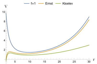
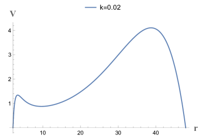
Figure 1: Left panel. The effective potential (16) in the equatorial plane for different metric functions. Right panel. The effective potential (16) in the equatorial plane for $k=0.02$ and $r\in[r_{-},r_{+}]$. The numerical values of the parameters are: $M=1$, $L=6$, $\varepsilon=1$, $B_{0}=0.04$.

One may discuss the trajectories for test particles evolving in the above potential, by numerically integrating the equations (11), (12) and (13), for specific orbital parameters.

In this respect, let us start with the case of the Melvin magnetic universe which has been largely discussed by [25]. In addition to the Lorentz interaction, the magnetic field exerts a gravitational force on the test particle. According to the author, there is not a significant difference to bound orbits in the absence of the black hole aside from a weaker gravitational force. Although some of the next results may be repetitive as done in previous work [25], they are given for comparison.

With $f=1$, the equations of motion (11) and (12) turn into the simpler expressions

$$\ddot{r} = -\frac{\Lambda,_{r}}{\Lambda}\left[\dot{r}^{2}+\frac{E^{2}}{\Lambda^{4}}\right]+r^{2}\left[\frac{\Lambda,_{r}}{\Lambda}+\frac{1}{r}\right]\dot{\theta}^{2}-\frac{2\Lambda,_{\theta}}{\Lambda}\dot{r}\dot{\theta}$$ (17)

$$-\frac{1}{r^{2}\sin^{2}\theta}\left[\frac{\Lambda,_{r}}{\Lambda}-\frac{1}{r}\right]\left[L-\frac{\varepsilon B_{0}r^{2}\sin^{2}\theta}{\Lambda}\right]^{2}-\frac{\varepsilon B_{0}}{\Lambda}\left[\frac{\Lambda,_{r}}{\Lambda}-\frac{2}{r}\right]\left[L-\frac{\varepsilon B_{0}r^{2}\sin^{2}\theta}{\Lambda}\right]$$

and

$$\ddot{\theta} = \frac{\Lambda,_{\theta}}{r^{2}\Lambda}\left[\dot{r}^{2}-\frac{E^{2}}{\Lambda^{4}}-r^{2}\dot{\theta}^{2}\right]-2\left[\frac{\Lambda,_{r}}{\Lambda}+\frac{1}{r}\right]\dot{r}\dot{\theta}-\frac{1}{r^{4}\sin^{2}\theta}\left[\frac{\Lambda,_{\theta}}{\Lambda}-\cot\theta\right]\left[L-\frac{\varepsilon B_{0}r^{2}\sin^{2}\theta}{\Lambda}\right]^{2}$$ (18)

$$-\frac{\varepsilon B_{0}}{r^{2}\Lambda}\left[\frac{\Lambda,_{\theta}}{\Lambda}-2\cot\theta\right]\left[L-\frac{\varepsilon B_{0}r^{2}\sin^{2}\theta}{\Lambda}\right]$$

and the effective potential (16) becomes:

$$V_{eff}(r,\theta)=\Lambda^{2}\left[1+\frac{\Lambda^{2}}{r^{2}\sin^{2}\theta}\left(L-\frac{\varepsilon B_{0}r^{2}\sin^{2}\theta}{\Lambda}\right)^{2}\right]$$ (19)

A numerical integration of the equations (17) and (18) allows us to display the polar plot of the bounded orbits of the test particle for different orbital parameters (see the figures 2 and 3). As it can be noticed in the figure 3, the particle can be confined to a bound orbit in the equatorial plane but under a small perturbation, the particle’s trajectory leaves the equatorial plane and describes a helicoid along the $z$ axis.

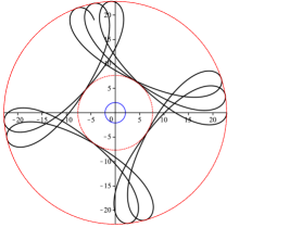
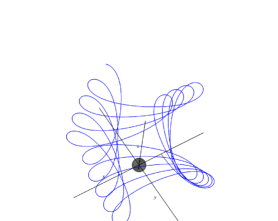
Figure 2: Left panel. Polar plot of bound orbits in the equatorial plane. Right panel. 3D plot of orbits. The numerical values are $\varepsilon=1$, $B_{0}=0.02$, $L=6$ and $E^{2}=1.22$.

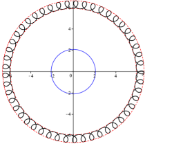
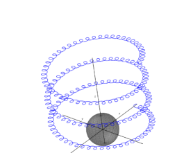
Figure 3: Left panel. Polar plot of bound orbits in the equatorial plane. Right panel. 3D plot of orbits. The numerical values are $\varepsilon=1$, $B_{0}=0.025$, $L=5$ and $E^{2}=1.06$.

An important characteristic which will be discussed in the following sections is that the particle’s timelike trajectory in the equatorial plane can curl up into a cycloidlike motion [25].

When the metric function in (4) describes a Schwarzschild BH, one deals with the Ernst spacetime [9] and the whole analysis becomes more complex. For an analytical investigation, one can take the range of the radial coordinate as being $r\gg 2M$ and employ a perturbative approach [4]. However, in the presence of quintessence, the linear term in the metric function (6) is linearly increasing with $r$ and this term might play a significant contribution for values of $r$ close to the cosmological horizon.

For the metric function (6) which is the aim of the present work, the particle’s trajectory can be obtained by numerically integrating the general equations (11), (12) and (13). As an example, in the figure 4, we represent the escape orbit of a particle and, for a comparison, we have kept the same numerical values as for the figure 2. Thus, the charged particles moving in the gravito-magnetic field in the presence of quintessence can escape the system in the $z-$direction or can be captured by the black hole.

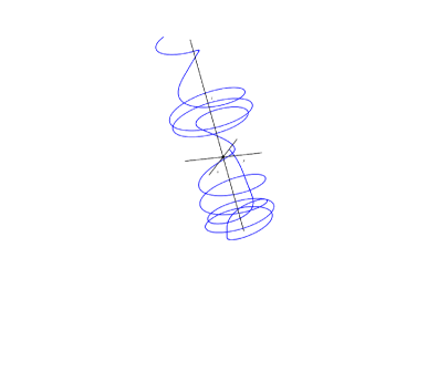
Figure 4: Escape orbit of a particle with energy $E^{2}=1.488$. Other numerical values are $M=1$, $k=0.01$, $\varepsilon=1$, $B_{0}=0.02$ and $L=6$.

At the end of this section, let us discuss the orbits in the equatorial plane for the metric function (6). For $\theta=\pi/2$, the function $\Lambda$ becomes:

$$\Lambda_{0}=1+B_{0}^{2}r^{2}$$ (20)

while the equations (13) and (11) have the expressions

$$\dot{\varphi}=\frac{\Lambda_{0}^{2}}{r^{2}}\left(L-\frac{\varepsilon B_{0}r^{2}}{\Lambda_{0}}\right)$$ (21)

and

$$\ddot{r}=\left(\frac{f^{\prime}}{2f}-\frac{\Lambda_{0}^{\prime}}{\Lambda_{0}}\right)\dot{r}^{2}-\frac{E^{2}}{\Lambda_{0}^{4}}\left(\frac{f^{\prime}}{2f}+\frac{\Lambda_{0}^{\prime}}{\Lambda_{0}}\right)+\frac{f}{r^{3}}\left(1-\frac{r\Lambda_{0}^{\prime}}{\Lambda_{0}}\right)\left(L-\frac{\varepsilon B_{0}r^{2}}{\Lambda_{0}}\right)^{2}$$

$$+\frac{f\varepsilon B_{0}}{\Lambda_{0}r}\left(2-\frac{r\Lambda_{0}^{\prime}}{\Lambda_{0}}\right)\left(L-\frac{\varepsilon B_{0}r^{2}}{\Lambda_{0}}\right)$$ (22)

The effective potential

$$V_{eff}(r)=f\Lambda_{0}^{2}\left[1+\frac{\Lambda_{0}^{2}}{r^{2}}\left(L-\frac{\varepsilon B_{0}r^{2}}{\Lambda_{0}}\right)^{2}\right]$$ (23)

is represented in the figure 5.

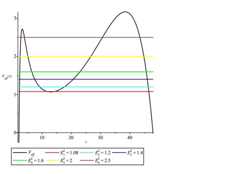
Figure 5: The effective potential (23) with parameters $M=1$,$k=0.02$, $\varepsilon=1$, $B=0.04$ and $L=9$.

As it can be noticed in the figures below, the potential (23) allows different different types of orbits, depending on the particle’s energy. The turning points are represented by dashed red circles, while the inner blue circle denotes the black hole horizon.

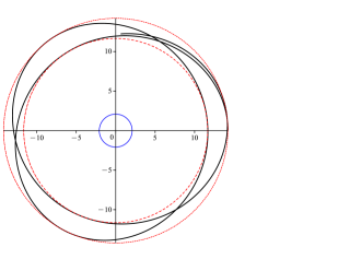
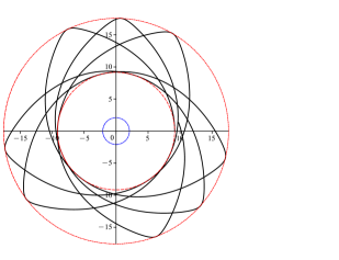
Figure 6: Left panel. Bound orbit of a particle with energy $E^{2}=1.08$ (red line in the Fig.5). Right panel. Bound orbit of a particle with energy $E^{2}=1.2$ (cyan line in the Fig.5)

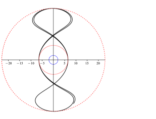
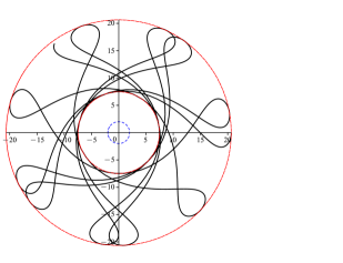
Figure 7: Left panel. Bound orbit of a particle with energy $E^{2}=1.4$ (blue line in the Fig. 5). Right panel. Bound orbit of a particle with energy $E^{2}=1.6$ (green line in the Fig.5)

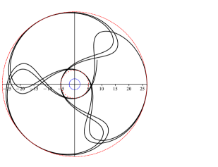
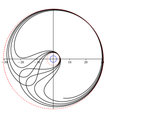
Figure 8: Left panel. Bound orbit of a particle with energy $E^{2}=2$ (yellow line in the Fig.5). Right panel. Bound orbit of a particle with energy $E^{2}=2.5$ (orange line in the Fig.5).

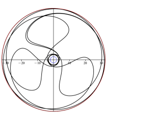
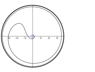
Figure 9: Left panel. First unstable circular orbit of a particle with energy $E^{2}=2.7167$. Right panel. Second unstable circular orbit of a particle with energy $E^{2}=3.1683$.

A particle moving near the first unstable circular orbit will either fall into the black hole or would evolve to a bound orbit between the outer turning point and the radius of first circular orbit as depicted in Fig 9, left panel. However in the case of the second unstable circular orbit, the particle either goes toward the cosmological horizon or falls into singularity, this solely depends upon the initial conditions, for instance see Fig. 9, right panel.

In the following section, we shall develop a purely analytic investigation and we consider ranges of the radial coordinate inbetween the two horizons where both $2M/r$ and $kr$ are acting like perturbations.

3 The weak magnetic field approximation

Near the horizon, the estimated strength of the magnetic field is much less the critical magnetic field that can influence the space-time of the black hole: $B\ll B_{G}\sim 10^{19}M_{S}/M$ (G) [6]. On the other hand, for charged test particles, the quantity $\varepsilon=q/m$ is very large and therefore the Lorentz force cannot be neglected even for weak magnetic fields.

Thus, in the followings, we consider the weak magnetic field approximation $\Lambda_{0}\approx 1$, meaning that the magnetic induction is too weak to influence the spacetime curvature but it acts on the charged particle through Lorentz interaction. In the equatorial plane $\theta=\pi/2$, the relations (13), (15) and (16) become

$$\dot{\varphi}=\frac{1}{r^{2}}\left[L-\varepsilon B_{0}r^{2}\right],$$ (24)

$$\dot{r}^{2}=E^{2}-V_{mag0}$$ (25)

and

$$V_{mag0}=f(r)\left[1+\frac{1}{r^{2}}\left(L-\varepsilon B_{0}r^{2}\right)^{2}\right]$$ (26)

with $f(r)$ given in (6). The particle’s trajectory can be obtained by integrating the relation

$$\frac{dr}{d\varphi}=r^{2}\sqrt{E^{2}-V_{mag0}}\left[L-\varepsilon B_{0}r^{2}\right]^{-1}$$ (27)

The potential (26) is reprersented in the left panel of the fig 10, for different values of the quintessence parameter $k$. One may notice that the effective potential is vanishing on the horizons. When the quintessence parameter $k$ is increasing, the second maximum of the potential disappears and the particle cannot be trapped on a bounded trajectory. An example of a bounded orbit in the equatorial plane is given in the right panel of the figure 10. The black circles correspond to the turning points $r_{1}$ and $r_{2}$, solutions of the equation $E^{2}=V_{mag0}$.

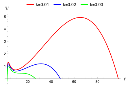
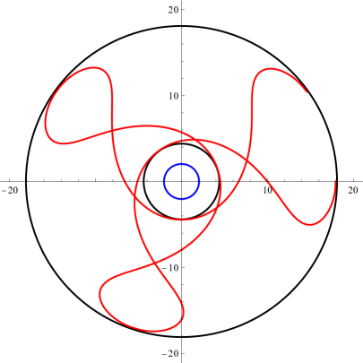
Figure 10: Left panel. The effective potential (26) for different values of the parameter $k$. Right panel. A bounded trajectory in the equatorial plane. The numerical values of the parameters are: $M=1$, $k=0.01$, $B_{0}=0.06$, $L=6$, $\varepsilon=1$, $E^{2}=1.1$.

As it can be noticed in the right panel of the figure 10, the presence of the magnetic field leads to a curly-type bounded orbit since $\dot{\varphi}$ defined in the equation (24) changes the sign in $r_{*}=\sqrt{L/(\varepsilon B_{0})}$ and $r_{*}\in[r_{1},r_{2}]$. For particles with positive $L$ and negative $\varepsilon$, $\dot{\varphi}$ is always positive and the corresponding trajectory has no curls.

3.1 Perturbed circular orbits in the equatorial plane

In the equatorial plane, the radial equation (11), in the weak field approximation $\Lambda_{0}=1$, can be written as

$$\ddot{r}\,=\frac{2f-rf^{\prime}}{2r^{3}}\left(L-\varepsilon B_{0}r^{2}\right)^{2}+\frac{2\varepsilon B_{0}f}{r}\left(L-\varepsilon B_{0}r^{2}\right)-\frac{M}{r^{2}}+\frac{k}{2}$$ (28)

One may notice that the Newtonian gravitational force $M/r^{2}$ directed along the radius toward the black hole considered in [4] is decreased by a constant quintessence contribution. In the particular case $\theta=\pi/2$ and $\Lambda_{0}=1$, one has the effective potential (26) and the relation (24).

The condition for a circular orbit $V^{\prime}_{mag0}(r_{0})=0$ leads to the following expression of the angular momentum

$$L=\left.\frac{r\left[-\varepsilon B_{0}r^{2}f^{\prime}\pm\sqrt{[4\varepsilon^{2}B_{0}^{2}f^{2}-{f^{\prime}}^{2}]r^{2}+2rff^{\prime}}\right]}{2f-rf^{\prime}}\right|_{r=r_{0}}$$

and one has to impose that the above expression is a real quantity for $f$ given in (6). A physical range for the circular orbit radius is $r_{0}\in[4M,\sqrt{2M/k}]$ and there are no constrains for $B_{0}$. Once $r_{0}>r_{*}=\sqrt{2M/k}$, the magnetic induction should exceed a minimum value so that $L$ is real. However, there is a maximum value of $B_{0}$ [26] and a maximum value of the quintessence parameter $k$ above which there are no stable circular orbits (see the left panel of the figure 10).

In the followings, we shall apply to (28) the procedure described in [4], where the Newtonian gravitational force $g=-M/r^{2}$ is considered as a perturbation for $r\gg 2M$. In our case, $g$ is replaced by $g_{k}=-M/r^{2}+k/2$ and we focus on the region of $r$ where bounded orbits exist and $g_{k}$ can be treated as a perturbation. For $r_{0}<r_{*}=\sqrt{2M/k}$, the quantity $g_{k}$ is negative, at $r_{0}=r_{*}$ it vanishes, while for $r_{0}>r_{*}$ it becomes positive.

As in [4], let us consider a point $(r_{0},\varphi_{0})$ and introduce the local Cartesian coordinates $(x,y)$ near it. For $x\ll r_{0}$ and $y\ll r_{0}$ one can work in the first order approximation

$$r\approx r_{0}+y\;,\quad\varphi\approx\varphi_{0}-x$$ (29)

with the radius $r_{0}$ obtained in the zero order approximation as being $r_{0}=\sqrt{L/(\varepsilon B_{0})}$. To first order in $x$, $y$ and $k$, the equations (28) and (24) lead to the following system of equations

$$\ddot{y}+\Omega^{2}y=-\gamma$$

$$\dot{x}=\frac{2\varepsilon B_{0}}{r_{0}}y$$ (30)

where we have introduced the notations

$$\gamma=\frac{M}{r_{0}^{2}}-\frac{k}{2}$$

$$\Omega^{2}=4\varepsilon^{2}B_{0}^{2}\left(1-\frac{2M}{r_{0}}-kr_{0}\right)$$ (31)

The solutions of the system (30) are given by the expressions

$$y(\tau)=-\frac{\gamma}{\Omega^{2}}+\eta\cos(\Omega\tau)$$

$$x(\tau)=-\frac{2\varepsilon B_{0}\gamma}{\Omega^{2}r_{0}}\tau+\frac{2\varepsilon B_{0}\eta}{\Omega r_{0}}\sin(\Omega\tau)$$ (32)

where $\eta$ is an integration constant and one has to consider $\eta\ll r_{0}$ so that the first order approximation is valid. The circular orbit is stable since the frequency $\Omega$ is real. One may notice that the quintessence parameter $k$ is affecting the frequency $\Omega$ and the value $\eta_{0}=\gamma/\Omega^{2}$ which separates the curly trajectory from the one without curls. For $r_{0}<r_{*}=\sqrt{2M/k}$, both $\gamma$ and $\eta_{0}$ are positive quantities, while for $r_{0}>r_{*}=\sqrt{2M/k}$, the parameters $\gamma$ and $\eta_{0}$ are negative. The line on the $(x,y)$ plane described by the solution (32) is called a trochoid and for $\eta=\eta_{0}$ it turns into a cycloid. In the left panel of the figure 11, we give the parametric plot of the trajectory corresponding to positive $\gamma$ defined in (31) and $\eta=2\eta_{0}=2\gamma/\Omega^{2}$. For a comparison, the blue line without curls corresponds to the case analyzed in [4], where $k=0$ so that $\gamma=M/r_{0}^{2}$ and $\Omega\approx 2\varepsilon B_{0}$. In the right panel we consider the case corresponding to $r>r_{*}$, for which $\gamma$ is negative and $\eta=\eta_{0}<0$.

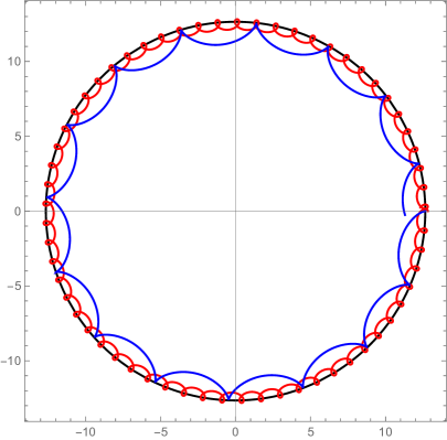
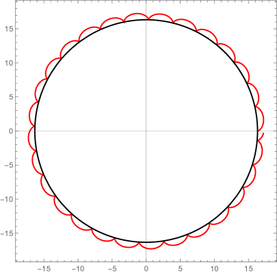
Figure 11: Left panel. The red graphic is the parametric plot of (29) with the solutions (32) for pozitive $\gamma$ defined in (31) and $\eta=2\eta_{0}=2\gamma/\Omega^{2}$. The numerical values of the parameters are: $k=0.01$, $L=8$, $\varepsilon=1$, $B_{0}=0.05$. The blue curve is for $k=0$ and $\eta=\eta_{0}$. Right panel. Parametric plot of (29) with the solutions (32) for $\gamma<0$. The numerical values of the parameters are: $k=0.01$, $L=8$, $\varepsilon=1$, $B_{0}=0.03$, $\eta=\eta_{0}<0$. The black circle represents the unperturbed circular orbit of radius $r_{0}=\sqrt{L/(\varepsilon B_{0})}$.

.

These curly trajectories are characteristic to charged particles moving in magnetic fields [25, 4]. One may notice in the figure 11 that the shape of the trajectory depends on how the terms $M/r_{0}^{2}$ and $k/2$ are related. As it can be noticed in the left panel of the figure 11, if the circular radius is $r_{0}<\sqrt{\frac{2M}{k}}$, the particle’s orbit would curl toward the black hole, as the attractive term dominates over the repulsive term.

In the particular situation when $r_{0}=\sqrt{\frac{2M}{k}}$ so that $\eta=0$, we recover the motion in a flat spacetime and the particle has a helicoidal trajectory as the one in the figure 3.

3.2 The three-dimensional approach

Secondly, let us analyze the more involved case of the general system of equations (11), (12) and (13), in the weak magnetic field approximation. For $\Lambda=1$, these equations get the expressions:

$$\ddot{r}\,=\,\frac{2f-rf^{\prime}}{2}r\dot{\theta}^{2}+\frac{2f-rf^{\prime}}{2r^{3}\sin^{2}\theta}\left[L-\varepsilon B_{0}r^{2}\sin^{2}\theta\right]^{2}+\frac{2\varepsilon B_{0}f}{r}\left[L-\varepsilon B_{0}r^{2}\sin^{2}\theta\right]-\frac{f^{\prime}}{2}$$

$$\ddot{\theta}\,=\,-\frac{2}{r}\dot{r}\dot{\theta}+\frac{\cot\theta}{r^{4}\sin^{2}\theta}\left[L-\varepsilon B_{0}r^{2}\sin^{2}\theta\right]^{2}+\frac{2\varepsilon B_{0}\cot\theta}{r^{2}}\left[L-\varepsilon B_{0}r^{2}\sin^{2}\theta\right]$$

$$\dot{\varphi}=\frac{1}{r^{2}\sin^{2}\theta}\left[L-\varepsilon B_{0}r^{2}\sin^{2}\theta\right]$$ (33)

and the effective potential reads

$$V=f(r)\left[1+\frac{\left(L-\varepsilon B_{0}r^{2}\sin^{2}\theta\right)^{2}}{r^{2}\sin^{2}\theta}\right]$$ (34)

In the first order approximation, one can consider

$$r\approx r_{0}+y\;,\quad\theta\approx\frac{\pi}{2}-z\;,\quad\varphi\approx\varphi_{0}-x$$ (35)

where $r_{0}=\sqrt{L/(\varepsilon B_{0})}$, in the zero order approximation. To first order in $x$, $y$ and $z$, the equations (33) lead to the system of equations (30) with the solutions (32) and to the $z-$equation

$$\ddot{z}=\frac{4\varepsilon^{2}B_{0}^{2}}{r_{0}}zy$$ (36)

i.e.

$$\ddot{z}+\frac{4\varepsilon^{2}B_{0}^{2}}{r_{0}}\left[\eta_{0}-\eta\cos(\Omega\tau)\right]z=0$$ (37)

where $\eta_{0}=\frac{\gamma}{\Omega^{2}}$. This is a Mathieu’s type equation whose general form is [27]

$$\ddot{z}+\left[a-2q\cos(2t)\right]z=0$$ (38)

the solutions being the Mathieu characteristic functions denoted as $ce_{n}(q,\tau)$ and $se_{n}(q,\tau)$, where $n$ is an integer. These are periodic functions, with the period $\pi$ or $2\pi$ and exist only for specific values of parameters $a$ and $q$.

In our case, the solutions of (37) are the Mathieu functions:

$$z(\tau)=C_{1}MathieuC\left[a,q,\frac{\Omega\tau}{2}\right]+C_{2}MathieuS\left[a,q,\frac{\Omega\tau}{2}\right]$$ (39)

with

$$a=\frac{16\varepsilon^{2}B_{0}^{2}\eta_{0}}{r_{0}\Omega^{2}}\;,\quad q=\frac{8\varepsilon^{2}B_{0}^{2}\eta}{r_{0}\Omega^{2}}.$$ (40)

The constants $a$ and $q$ are usually referred as characteristic number and parameter, respectively. From the general theory of the Mathieu’s functions [27], we know that these are of the form

$$u\sim e^{irx}g(x)\,,$$

where $g(x)$ is a periodic function. Depending on the parameters $a$ and $q$, the so-called Mathieu Characteristic Exponent $r$ may be real or imaginary. When $r$ becomes imaginary, the real and imaginary parts of the Mathieu functions are exponentially growing as a result of a parametric resonance. Even though there exists a comprehensive literature about the Mathieu equation and its solutions, the crucial problem is to find conditions for the parameters such that the solutions remain bounded. The stability charts give the transition curves in the parameters plane which separate the regions corresponding to a stable motion from those of instability.

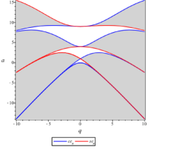
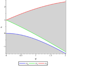
Figure 12: Stability chart for the Mathieu equation (38). Stability regions are the white areas, while the grey ones correspond to instability regions.

In our case, for a given value of $a$, using the diagrams as the ones represented in the figure 12, we find the range of $\eta$ so that the corresponding $q$ is in a stability region. For $r_{0}<r_{*}=\sqrt{2M/k}$, the parameters $a$ and $q$ are positive quantities and there are large regions of stability.

In the figure 13, in the left panel, we give the 3-dimensional parametric plot corresponding to the solutions (32, 39) and the projection on the $xy$ plane is given in the right panel. For the chosen numerical values, one has $a=0.077$ and $q=0.15$ and therefore we are in the first stability region.

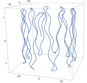
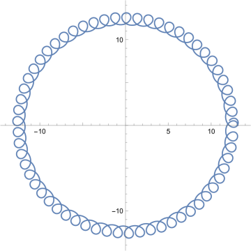
Figure 13: Left panel. Three dimensional parametric plot with the solutions (32, 39) . Right panel. The projection on the $xy-$plane. The numerical values of the parameters are: $k=0.01$, $L=8$, $\varepsilon=1$, $B_{0}=0.05$, $\eta=0.7>\eta_{0}$

Once $r_{0}>r_{*}$ and $\gamma$ in (31) becomes negative, the parameter $a$ of the Mathieu functions is also negative. In this situation, for a given $a-$ value, there are very narrow ranges for the parameter $q$ where the solutions are stable and bounded, as it can be noticed in the figure 12.

4 Conclusions

The present paper deals with charged particles motion around a Schwarzschild black hole immersed in an axisymmetric magnetic field, in the presence of quintessential matter. A comparison with the charged particles trajectories in the Melvin magnetic universe [25] is pointing out the existence, in both cases, of curly trajectories which is characteristic for the charged particles experiencing an inward gravitational force which is counteracted by an outwards Lorentz force.

Starting with the general Lagrangian (8), we derive the field equations and the effective potential whose plot gives us important information on the allowed regions of motion and equilibrium points. The field equations are not exactly solvable and we have used numerical methods to represent the trajectories in the figures 2, 3, and 4.

In particular cases, the explicit form of geodesic motion can be obtained in terms of elliptic integrals [28]. In our case, the equations (11), (12), (13) were solved numerically by using the Maple software and implementing a Runge-Kutta algorithm of 4th order. As a consistency check we used the relation (15).

A special attention is given to the case of a weak magnetic field which can be analytically treated. Firstly, we have considered the orbits in the equatorial plane. The gravitational force $M/r^{2}$ directed toward the black hole is decreased by a constant quintessence contribution and bounded trajectories exist only for low values of the quintessence parameter. For circular orbits, the perturbative approach reveals a cycloidlike or trochoidlike motion, similar to those found by Frolov [4] and Lim [25] in Ernst spacetime. However, one may notice in the figures 11 that the shape of the perturbed circular trajectory is dictated by the parameter $\gamma$ whose sign reflects the relation between the attractive gravitational force and the repulsive contribution induced by the presence of quintessential matter. The quintessence parameter value is affecting the frequency of the circular motion as well as the transition from a curly to a non-curly trajectory.

Secondly, we have turned to a three-dimensional investigation and worked out, in the first-order approximation, the general system of equations (33). The radial equation reduces to that of a harmonic oscillator driven by a periodic driving force, while the perturbed motion in the $\theta$ direction is governed by a Mathieu-type equation. For $r_{0}<r_{*}=\sqrt{2M/k}$, one may find large ranges for the model’s parameters for which the Mathieu’s functions are bounded and stable. This means that the corresponding orbit of radius $r_{0}$ is indeed stable even when the particles are perturbed slightly away from the equator (see the figure 13). On the other hand, when the quintessence contribution becomes dominant and $kr_{0}>2M/r_{0}$, there are very narrow stability ranges for the Mathieu’s parameters. Outside these stability regions, the Mathieu’s Characteristic Exponent is complex and the corresponding Mathieu’s functions are exponentially increasing. This means that even though the orbit of radius $r_{0}$ corresponds to a minimum value of the potential, the trajectory is unstable when the particle is slightly perturbed away from the equatorial plane.

Our results agree with the ones derived in [29, 30], where the small radial and latitudinal oscillations around a stable equatorial orbit have been discussed in detail. Also, the case of the movement confined in the equatorial plane has been investigated in [4]. The main conclusion is that even though there is a clear resemblance to the Larmor precession in a pure magnetic field, the effect of a weak external uniform magnetic field combined with a gravitational or/and a quintessence force may be substantial.

References

- [1] Planck Collaboration (N. Aghanim et al.), Astron. Astrophys. 596 (2016) A105
- [2] R. P. Eatough et al., Nature 501(7467) (2013) 391
- [3] R. M. Wald, Phys. Rev. D 10 (1974) 1680
- [4] V. P. Frolov and A. A. Shoom, Physical Review D, 82(8) (2010) 084034
- [5] J. C. McKinney and R. Narayan, Mon. Not. Roy. Astron. Soc. 375 (2007) 523
- [6] R. A. Daly, The Astrophysical Journal, 886 (1) (2019) 37
- [7] M. Yu. Piotrovich, A. G. Mikhailov, S. D. Buliga and T. M. Natsvlishvili. arXiv e-prints: arXiv:2004.07075 (2020)
- [8] S. Kenzhebayeva et al., Phys. Rev. D 109(6) (2024) 063005
- [9] F. J. Ernst, Journal of Mathematical Physics, 17(1) (1976) 54
- [10] D. Clowe et al., Astrophys. J. Lett. 648(2) (2006), L109
- [11] R. Abuter et al. (GRAVITY Collaboration), Astron. Astrophys. 636 (2020) L5
- [12] S. Capozziello et al., Class. Quant. Grav. 23(4) (2006) 1205
- [13] A. Vikman, Phys. Rev. D 71(2) (2005) 023515
- [14] V. V. Kiselev, Class. Quantum Gravity 20(6) (2003) 1187
- [15] S. Fernando, General Relativity and Quantum Cosmology 44 (2012) 1857
- [16] A. Al-Badawi, S. Kanzi and I. Sakalli, Eur. Phys. J. Plus 135(2) (2020) 219
- [17] M. A. Dariescu, V. Lungu, C. Dariescu, C. Stelea, Phys. Rev. D, 109 (1) (2024) 024021
- [18] M. A. Dariescu, C. Dariescu, V. Lungu and C. Stelea, Phys. Rev. D 106 (6) (2022) 064017
- [19] V. Cardoso et al., Phys. Rev. D 105 (6) (2022) L061501
- [20] C. Stelea, M. A. Dariescu and C. Dariescu Phys. Lett. B, 847 (2023) 138275
- [21] C. Stelea, M. A. Dariescu and C. Dariescu, Phys. Rev. D 98(12) (2018) 124022
- [22] C. Stelea, M. A. Dariescu and C. Dariescu, Phys. Rev. D 97 (10) (2018) 104059
- [23] C. Stelea, M. A. Dariescu and C. Dariescu, Phys. Rev. D 108 (8) (2023) 084034
- [24] S. S. Yazadjiev, Mod. Phys. Lett. A 20 (2005) 821
- [25] Y. K. Lim, Physical Review D, 91(2) (2015) 91.024048
- [26] E. P. Esteban, Il Nuovo Cimento B Series 11, 79(1) (1984) 76
- [27] M. Abramowitz and I. A. Stegun (Eds.). ”Mathieu Functions.” in Handbook of Mathematical Functions with Formulas, Graphs, and Mathematical Tables, 9th printing. New York: Dover, 1972
- [28] E. Battista and G. Esposito, Eur. Phys. J. C 82 (2022) 1088
- [29] M. Kolos, Z. Stuchlik and A. Tursunov, Class. Quant. Grav. 32 (2015) 165009
- [30] M. Kolos, M. Shahzadi and A. Tursunov, Eur. Phys. J.C 83 (4) (2023) 323.