Time-dependent Hamiltonians and Geometry of Operators Generated by Them

Abstract

We obtain the complexity geometry associated with the Hamiltonian of a quantum mechanical system, specifically in cases where the Hamiltonian is explicitly time-dependent. Using Nielsen’s geometric formulation of circuit complexity, we calculate the bi-invariant cost associated with these time-dependent Hamiltonians by suitably regularising their norms and obtain analytical expressions of the costs for several well-known time-dependent quantum mechanical systems. Specifically, we show that an equivalence exists between the total costs of obtaining an operator through time evolution generated by a unit mass harmonic oscillator whose frequency depends on time, and a harmonic oscillator whose both mass and frequency are functions of time. These results are illustrated with several examples, including a specific smooth quench protocol where the comparison of time variation of the cost with other information theoretic quantities, such as the Shannon entropy, is discussed.

I Introduction

The quantity computational complexity of a given quantum state roughly measures the minimum number of basic gates required to build the target state starting from an initial reference state. Among various measures to quantify computational complexity, one of the most commonly used is the one proposed by Nielsen and collaborators Nielsen1 ; Nielsen2 ; Nielsen3 . In this approach, the reference and target states correspond to two points on a curved manifold, and all the possible unitary transformations that connect these two points are assigned with a cost function. According to this geometric formulation, the path that minimises the cost function is nothing but the geodesic on that manifold of the unitary operator, and the length of the geodesic is called the Nielsen complexity (NC). This particular measure of complexity has been explored in significant detail in recent literature not only because it can shed light on fundamental aspects of the information contained in a quantum state Myers1 ; BSS ; KKS ; Myers2 ; HM ; BMS ; BS ; Caceres:2019pgf , but also due to the fact that NC can also be used an important probe of quantum quenches ABHKM ; Gautam:2022gci ; Pal:2022rqq ; Chandran:2022vrw ; Camargo:2018eof , quantum phase transitions LWCLTYGG ; JGS ; XYZ ; SK ; JGS2 ; PPS ; WH ; Roca-Jerat:2023mjs ; Jaiswal:2024yts ; Jayarama:2022xta , and quantum chaos BDKP1 ; BDKP2 ; HJU ; Qu:2022zwq , and has various other applications as well Pal:2021jtm ; Chowdhury:2023iwg ; Adhikari:2021ckk ; Basteiro:2021ene ; Camilo:2020gdf ; Erdmenger:2020sup . Specifically, typical behaviour of circuit complexity has been used in ABHKM ; Camargo:2018eof ; Pal:2022rqq ; Gautam:2022gci ; Chandran:2022vrw to understand the unitary dynamics of an isolated quantum system, when the system is taken out of equilibrium by means of a single or multiple sudden or smooth quenches thereby changing the parameters of the Hamiltonian according to different relevant time scales. It has also been used in various works as an important quantum information theoretic tool to detect the zero temperature quantum phase transition in various contexts and models, where typically the discontinuity of the complexity marks the quantum critical point LWCLTYGG ; JGS ; XYZ ; SK ; JGS2 ; PPS ; WH ; Roca-Jerat:2023mjs ; Jaiswal:2024yts ; Jayarama:2022xta . Apart from the NC, there are also other important measures of circuit complexity of quantum states which differ from Nielsen’s approach in many aspects (e.g., the one introduced in CHMP by using the Fubini-Study metric associated with a pure quantum state), however, in this paper, we shall mostly consider Nielsen’s formulation. For a recent review of different approaches to circuit complexity and its application in holography, we refer to Chapman:2021jbh .

It is important to note that, apart from the given target and reference states, the NC crucially depends on the choice of the cost function associated with each of the unitary paths on the manifold. Though the qualitative nature of NC in a quantum system strongly depends on the choice cost function, in Nielsen’s original formulation, this choice remains arbitrary (for an exposition on different cost functions used in this context, we refer to BMS ). Another built-in aspect of NC is the fact that the unitary complexity geometry associated with NC is either right or left invariant under a global transformation of the unitary operator which determines the geometry. As was pointed out in YK ; YK2 ; YANZK ; YANZK2 , for a physical quantum system, this fact is somewhat unsatisfactory since, e.g., the Nielsen complexity geometry corresponding to two Hamiltonians related by a unitary transformation would be different, and hence unacceptable from a physical point of view since they describe the same quantum system. Based on the assumption that NC and hence the cost function should be invariant under both left and right unitary transformation of the generator associated with a given path on the unitary manifold, the notion of bi-invariant complexity was proposed in YK ; YANZK ; YANZK2 . In this paper we mainly consider this bi-invariant formulation of the NC, and apply it to the Hamiltonians of some well known quantum mechanical systems.

Usually, in the problem of calculating NC (or other notions of circuit complexity), the following situation is considered - the reference and target quantum states are given (along with the chosen cost functional and penalty factors for any gate directions, if any), and one has to minimise the costs associated with all the relevant unitary curves to find the NC. However, in this problem, the instantaneous generator of the unitary curve is not commonly given specific importance because we are only interested in the length of the geodesic curve (i.e., complexity). Consider now a different posing of the above-mentioned problem, which is equally important: the time evolution of an initial reference under the Hamiltonian of a given quantum system. In that case, the unitary operator is the time evolution operator itself, and the target state is actually some time-evolved state for a particular value of time. Of course, any arbitrary target state may not be on the unitary curve generated by the system Hamiltonian, and consequently, those states are not achievable under this protocol. To explain further, suppose, one can choose only two from the three quantities: a reference state, a target state, and Hamiltonian that generates the evolution, and third one is naturally constrained by a unitary evolution. In the standard way of defining NC, the first two (i.e., reference and target states) are given, whereas here we are interested in the scenario where the first and third options (i.e., reference state and system Hamiltonian) are pre-assigned. As a natural consequence of the preceding statement, the nature of the parameter associated with the unitary curve connecting the reference and target state is different from the usual treatment of NC. Specifically, in this paper, we construct a bi-invariant geometry associated with the operators generated by the Hamiltonian of quantum mechanical systems. One of the most important such operators is the time evolution operator itself, and in that case, the parameter along the unitary path is time. In summary, our goal here is to calculate the cost of operators along the time evolution curve of a quantum mechanical system by using the framework of bi-invariant complexity geometry (CG).

The quantum mechanical systems we mainly focus on have Hamiltonians which are explicit functions of time, and their associated Hilbert space is infinite-dimensional. These two characteristics (explicit time dependence and infinite-dimensional Hilbert space) of the Hamiltonian have important bearings on the cost associated with time-evolution operators. Firstly, due to the fact the generator (here the Hamiltonian) is an explicit function of the parameter (the time), and since the CG is bi-invariant, the unitary curve is not a geodesic (note that the geodesic curves on a bi-invariant geometry are determined by generators which are constant along these trajectories). Therefore, in this set-up it is only meaningful to consider the total cost along the given curve, not the minimum among a set of such costs computed along a collection of trajectories connecting a given target and reference state. Secondly, due to the infinite-dimensional Hilbert space associated with the generator of the unitary curve, to obtain a meaningful expression of the cost we need to suitably regularise it. Here we roughly follow the method outlined in YK for the case of time-independent Hamiltonians and suitably generalise it for cases when the generator is explicitly time-dependent.

Summary of the paper. We now summarise the content and main results obtained in the rest of the paper. In the next section, we shall briefly review the geometric formulation of the circuit complexity pioneered by Nielsen. Also, we shall introduce the bi-invariant CG and the cost that will be used in the rest of the paper. In section III we use this cost function to obtain the CG associated with time-independent Hamiltonians, where we also discuss the procedure of regularising these costs. In that section we also show how the addition of an extra linear force term in the Hamiltonian can be interpreted as a trace regulator, thereby providing a physical justification for such method. Since for the examples considered in this section, the Hamiltonian is time-independent, the corresponding time-evolution is actually a geodesic in the bi-invariant geometry, and hence, the cost computed along such a trajectory is the bi-invariant complexity itself.

Section IV deals with the computation of the bi-invariant CG associated with a harmonic oscillator (HO) Hamiltonian whose frequency depends on time. One of the main ingredients of our analysis is the eigenfunctions of the time-dependent invariant operator which arises in a formulation developed by Lewis and Riesenfeld LR ; DR . By using the matrix elements of the Hamiltonian in such a wavefunction basis, we obtain a compact analytical formula for the regularised cost function (see eq. (57)), which constitutes one of the main results of this paper. We also show how this time-dependent cost reduces to the more familiar expression for the cost function of a usual HO in the appropriate limit and obtain a bound on the total cost evaluated along the time-evolution curve up to a certain finite time (see eq. (61)).

In Section V, we generalise the results of section IV for the case of the Hamiltonian of an oscillator whose both mass and frequency changes with time. For this Hamiltonian also, we are able to provide an analytical formula for the regularised cost function by using the Lewis - Riesenfeld theory of time-dependent invariant operators. The fact that such a Hamiltonian is actually an element of the $su(1,1)$ Lie algebra provides a way of directly obtaining the exact form of the time evolution operator using techniques of Lie group theory. Using this exact expression for the time-evolution operator, we show that suitably redefining the time parameter, it is possible to map the time evolution operator of an oscillator with time varying mass and frequency to an oscillator with unit mass but time varying frequency. Furthermore, we show that under the same reparametrisation, the total bi-invariant cost evaluated along the time-evolution curves of these two oscillators can be mapped to each other.

We discuss the significance of our results in section VI, and indicate a few possible future directions. This paper also contains two appendices: in Appendix. A we compute the bi-invariant cost and compare it with other measures, such as the change in Shannon entropy for one of the most common physical situations where time-dependent Hamiltonians are used, namely that of a smooth quantum quench, whereas in Appendix. B we provide some details of the computation of the time-evolution operator associated with Hamiltonians which are elements of the $su(1,1)$ Lie algebra.

II Cost functional and the circuit complexity in Nielsen’s approach

In this section we briefly review Nielsen’s geometric approach of calculating the circuit complexity Nielsen1 ; Nielsen2 ; Nielsen3 . Suppose, for a quantum system we are given a set of unitary operators, and we want to prepare a state $\big{|}\psi_{T}\big{>}$, known as the target state, starting from a given reference state $\big{|}\psi_{R}\big{>}$. In the problem of calculating the circuit complexity we consider the following question. What is the minimum number of operators within this set that we require to accomplish this transformation? This is known as the computational complexity of preparing the state $\big{|}\psi_{T}\big{>}$ from $\big{|}\psi_{R}\big{>}$ denoted as $\mathcal{C}\Big{(}\big{|}\psi_{R}\big{>}\rightarrow\big{|}\psi_{T}\big{>}\Big{)}$.

In Nielsen’s approach, one considers a state infinitesimally different from the reference state such that a unitary operator can produce the former starting from the latter with an infinite accuracy. We denote the unitary operator connecting the reference and the target state to be $O$, i.e. $\big{|}\psi_{T}\big{>}=O\big{|}\psi_{R}\big{>}$. Nielsen’s approach is to consider a space of such unitary operators on which the identity operator and the required operator $O$ can be thought to be connected by a continuous curve $c(s)$, parameterised by some affine parameter $s$. Thus, each point on such a curve represents a unitary operator $c(s)$, and we parameterise the path in such a way that its starting point (the identity operator) is at $s=0$ and the final point (the operator $O$) corresponds to $s=1$. Hence, $c(s=0)=\mathbf{I}$ and $c(s=1)=O$.

A quantity important for our purposes is the so-called instantaneous Hamiltonian $H(s)$ BMS , which is nothing but the generator of the infinitesimal translation along the curve $c(s)$ and hence, satisfies the usual relation

$$i\frac{dc(s)}{ds}=H(s)c(s)~{}.$$ (1)

Given an arbitrary state $\big{|}\psi(s)\big{>}$, the action on it by $H(s)$ takes it to a nearby state ($\big{|}\psi(s+ds)\big{>}$) infinitesimally different from it. Therefore, the instantaneous state $\big{|}\psi(s)\big{>}$ satisfies following the Schrodinger like equation

$$i\frac{d\big{|}\psi(s)\big{>}}{ds}=H(s)\big{|}\psi(s)\big{>}~{}.$$ (2)

For quantum systems, this equation is the same as the Schrodinger equation where the system Hamiltonian explicitly depends on time $t$ (in that case, the parameter we call $s$ is just the time) and equivalently, Eq. (1) is the same as that is satisfied by the time evolution operator $\mathcal{U}(t)$. This analogy with the time evolution operator directly indicates a way of writing the operator $c(s)$ as a path-ordered integral over the Hamiltonian $H(s)$ as

$$c(s)=\overleftarrow{\mathcal{P}}\exp\bigg{[}-i\int_{0}^{s}H(s^{\prime})\text{d}s^{\prime}\bigg{]}~{}.$$ (3)

This identification is very useful for our purposes since it enables us to calculate the NC of such time evolution operators generated by the Hamiltonians of the time-dependent quantum systems.

There are infinitely many different continuous paths connecting the identity with the desired operator $O$, and in Nielsen’s approach, the next step is to associate a certain computational cost with each of them by defining a cost function $F\big{(}c(s),~{}H(s)\big{)}$, which can, in general, depend on both the unitary curve and the generator. Then, the NC of creating the operator $O$ starting from the identity is obtained by minimising the cost functional (which is the integral of the cost function over a specific curve $c(s)$). Mathematically, to find out the NC of an operator $O$ starting from the identity operator we need to solve the following minimisation problem,

$$\mathcal{C}\big{(}O\big{)}=\min\int_{0}^{1}F\big{(}c(s),~{}H(s)\big{)}\text{d}s~{}~{}~{}\text{with}~{}~{}c(s=0)=\mathbf{I}~{},~{}\text{and}~{}~{}c(s=1)=O~{}.$$ (4)

Now there can be many such operators $O_{i}$, belonging to the general set $O$, which connects the final state $\big{|}\psi_{T}\big{>}$ with the initial state $\big{|}\psi_{R}\big{>}$. The NC of preparing $\big{|}\psi_{T}\big{>}$ from $\big{|}\psi_{R}\big{>}$ is the minimum value of the complexity of all such operators BS i.e.

$$\mathcal{C}\Big{(}\big{|}\psi_{R}\big{>}\rightarrow\big{|}\psi_{T}\big{>}\Big{)}=\min\Big{\{}\mathcal{C}(O_{i})~{}|~{}\forall O_{i}~{}\in O~{},~{}\big{|}\psi_{T}\big{>}=O\big{|}\psi_{R}\big{>}~{}~{}\Big{\}}~{}.$$ (5)

In this paper we mainly consider the NC and its associated geometry (to be described below) of those operators for which the generator in Eq. (3) is that of the Hamiltonian of some quantum system.

Though in Nielsen’s original formalism there are no physical principles by which these cost functions can be fixed, nevertheless, one can choose the cost function in such a way that it satisfies some generic properties such as smoothness, continuity, positivity, and positive homogeneity. Furthermore, $F$ can be chosen in such a way that it satisfies the triangle inequality for the sum of two Hamiltonians (see Nielsen1 ; Myers1 for a detailed discussion of these properties of the cost). When the cost is chosen so that it obeys these requirements the complexity in Eq. (4) actually represents the length of a geodesics on a Finsler manifold. However, even after imposing all these requirements on the cost, it is not unique. In literature there are many choices for these cost functions, which are sometimes chosen in such a way that the final expression for the NC comes with some required scaling behaviours, see, e.g., Myers1 ; Myers2 ; CHMP . For a summary and relative merits and demerits of different instantaneous state-independent and state-dependent cost functions used in the literature, see BMS .

As mentioned above, since the unitary operators we shall consider in this paper are generated by the Hamiltonian of some quantum system, we assume that the Hamiltonian can be written in terms of a basis $\{e_{I}\}$, with respective coefficients denoted as $Y^{I}$, i.e. $H=e_{I}Y^{I}$. In terms of these coefficients, two popular state-independent cost functions used widely in the literature are

$$F_{2}=\Big{[}\sum_{I}\Big{(}Y^{I}(s)\Big{)}^{2}\Big{]}^{1/2}~{}~{},~{}~{}\text{and}~{}~{}F_{\kappa}=\sum_{I}\big{|}Y^{I}(s)\big{|}^{\kappa}~{}~{}.$$ (6)

The first one of the above cost functions, as well as the second one with $\kappa=1$ were originally proposed by Nielsen, while the second class of costs with $\kappa>1$ were proposed in Myers1 . As pointed out in BMS , there is a problematic issue with all these costs, namely, unless one imposes certain extra criteria on the bases used in expanding the instantaneous Hamiltonian, the geometry resulting from two different choices of this basis do not in general coincide. The simplest such condition one can impose is $\text{Tr}\big{[}e_{I}.e_{J}\big{]}=N\delta_{IJ}$, $N$ being an overall normalization constant.

The construction described above naturally represents a geometry in the space of unitaries, known as the CG. To see this, we write down an element of the unitary curve in the following suggestive way (see Eq. (4))

$$\text{d}l^{2}=F^{2}\big{(}c(s),H(s)\big{)}\text{d}s^{2}=g\big{(}H(s),H(s)\big{)}\text{d}s^{2}~{}.$$ (7)

Written in terms of the basis $\{e_{I}\}$, defined above we then have the metric components of the CG to be

$$F^{2}\big{(}H(s)\big{)}=g_{IJ}Y^{I}Y^{J}~{}.$$ (8)

This formula clearly indicates that the cost function actually gives norm of the instantaneous Hamiltonian YK . Therefore, below, we sometimes use these two words interchangeably.

Now we come back to the problem of defining such a geometry uniquely. Besides the above mentioned problem of nonuniqueness of the CG, there is one additional feature of such constructions - the resulting geometry is only right (or left) invariant under a global transformation of the unitary operator. As discussed in detail in YANZK ; YANZK2 ; YK , this property is somewhat problematic for defining complexity associated with a quantum mechanical Hamiltonian, since a unitary transformed system is identical to that of the original system, in the sense that physical observables computed from both of them make identical predictions for the original system and the transformed one. Hence, it is very much desirable that for an arbitrary unitary operator $U(s)$, defined on the CG, the cost function or the norm should be such that it is invariant under the unitary transformation of the Hamiltonian, i.e.,

$$F\big{(}H(s)\big{)}=F\big{(}U(s)H(s)U^{\dagger}(s)\big{)}~{},$$ (9)

and as was shown in YANZK , this property, in turn, guarantees that the resulting NC is invariant under such a transformation. This property of the CG is called bi-invariance. By requiring that CG associated with a quantum system be bi-invariant, the following class of cost functions has been obtained in YANZK ; YANZK2

$$F\big{(}H(s)\big{)}=\lambda_{0}\bigg{[}\text{Tr}\Big{[}\big{(}H(s)H^{\dagger}(s)\big{)}^{p/2}\Big{]}\bigg{]}^{1/p}~{},$$ (10)

where the constant $p$ takes positive integer values, and $\lambda_{0}>0$ is an overall constant multiplier. The resulting cost function is known as the Schatten norm.

In this paper we shall consider the above norm with $p=2$, since as argued in YANZK2 , the expression for cost function (and the resulting expression for the NC) for different values of $p$ are quantitatively the same, only their numerical values are different. The aim of this paper is to calculate the cost of operators generated by the Hamiltonian of a quantum system, both time-independent and explicitly time-dependent cases, with a specific focus given to the latter case due to its more involved nature.

III Complexity geometry associated with time-independent Hamiltonians

We now discuss the construction of the bi-invariant CG of operators generated by the Hamiltonian of some well-known quantum systems. In this section we consider the case when the Hamiltonian is time-independent, while in the next section, and the rest of the paper, we deal with systems whose Hamiltonians are explicit functions of time. The instantaneous Hamiltonian appearing in Eq. (2) is the ordered Hermitian Hamiltonian operator (which we denote as $\mathbf{H}$ in the followings) of a given quantum system, and this equation is nothing but the Schrodinger equation for the time evolution of the state $\big{|}\psi(t)\big{>}$. Furthermore, the unitary operator of our concern is the time evolution operator generated by the system Hamiltonian. At this point, we stress that we want to evaluate the computational cost along the time evolution curve $\mathcal{U}(t)$, not the NC of a time evolved state (or an operator on the time evolution curve) - this fact makes our analysis different from other works where time evolution of NC corresponding to different quantum systems have been reported BDKP1 ; YK2 ; HJU . Specifically, in our set-up, the parameter $s$ characterising the curves in the space of unitary operators is time $t$.

When $p=2$, with the Hamiltonian operator as the generator, the cost functions in Eq. (10) reduce to

$$F^{2}\big{(}\mathbf{H}(s)\big{)}=\lambda_{0}^{2}\text{Tr}\big{[}\mathbf{H}^{2}(s)\big{]}~{}.$$ (11)

This cost represents the length on a Riemannian metric, which is nothing but the Cartan-Killing metric corresponding to the Lie group associated with the quantum system RG ; FSS . As we shall see, for the cases we consider in this paper, the Hamiltonian is an element of some Lie algebra, and the above mentioned Lie group is associated with this algebra. Clearly, to find out the CG using this cost, we need to calculate the trace of the squared Hamiltonian. However, the Hilbert spaces associated with the systems we are going to consider are infinite dimensional, and hence the trace can be divergent. A procedure of obtaining the CG by suitably regularizing the trace of the Hamiltonian operator using the Hurwitz $\zeta$ functions was described in YK . For later purposes, we first briefly review this procedure and its application to find out the CG of a generalised oscillator, as worked out in YK . We can also provide an alternative interpretation of this regularization in terms of a constant driving force present in the original Hamiltonian (see subsection III.2).

The first step is to calculate the “mean value” of the Hamiltonian $\mathbf{H}$ (denoted here by $a$), by imposing the following condition on the trace

$$\text{Tr}\big{[}\mathbf{H}-a\mathbf{I}\big{]}=0~{}.$$ (12)

We refer to this condition as the regularization condition in the following. Since this is an $U(1)$ transformation, the addition by $-a\mathbf{I}$ does not alter the CG, i.e. the bi-invariant geometry generated by the original Hamiltonian $\mathbf{H}$ is the same as the one generated by the displaced Hamiltonian $\tilde{\mathbf{H}}=\mathbf{H}-a\mathbf{I}$ YK . With $a$ determined from the above condition, the regularised value of the cost in Eq. (11) is given by the trace of the squared displaced Hamiltonian (the subscript $r$ implies regularised)

$$F^{2}_{r}\big{(}\mathbf{H}\big{)}=\lambda_{0}^{2}\text{Tr}\big{[}\big{(}\mathbf{H}-a\mathbf{I}\big{)}^{2}\big{]}~{}.$$ (13)

To evaluate this quantity, we first denote the diagonal matrix elements of $\mathbf{H}$ with respect to a complete set of orthonormal eigenfunctions $\big{|}\psi_{n}\big{>}$, which diagonalise the Hamiltonian, as $E_{nn}$. These are just the energy eigenvalues for time-independent Hamiltonians considered in this section. Then, one defines the analytic continuation of the sum

$$\zeta_{\mathbf{H}}(k)=\sum_{n=0}^{\infty}\frac{1}{\big{(}E_{nn}\big{)}^{k}}~{}$$ (14)

as the $\zeta$ function associated with the Hamiltonian. Now it is easy to see that the trace of the Hamiltonian is just $\zeta_{\mathbf{H}}(-1)$. Similarly, for the displaced Hamiltonian $\tilde{\mathbf{H}}=\mathbf{H}-a\mathbf{I}$, the associated $\zeta$ function can be written as

$$\zeta_{\tilde{\mathbf{H}}}(k)=\sum_{n=0}^{\infty}\frac{1}{\big{(}E_{nn}-a\big{)}^{k}}~{}~{}.$$ (15)

Hence, the regularised trace of the Hamiltonian is given by $\zeta_{\tilde{\mathbf{H}}}(-1)$. The last step of finding out the regularised cost is to recognise that it can be written in terms of the above zeta function as

$$F^{2}_{r}\big{(}\mathbf{H}\big{)}=\lambda_{0}^{2}\text{Tr}_{r}\big{[}\big{(}\mathbf{H}-a\mathbf{I}\big{)}^{2}\big{]}~{}~{}=\lambda_{0}^{2}\zeta_{\tilde{\mathbf{H}}}(-2)~{}.$$ (16)

As we shall see, the last two expressions can be evaluated in terms of the Hurwitz $\zeta$ function, which is defined as the analytic continuation of the sum

$$\zeta(k,q)=\sum_{n=0}^{\infty}\frac{1}{(n+q)^{k}}~{}~{}.$$ (17)

To illustrate the above procedure, the quantum systems we now consider are the following: the first one is a generalised oscillator and the second one is an isotonic oscillator where, apart from a simple harmonic term, an additional singular inverse square term is also present in the total potential. The CG generated by such Hamiltonians can be obtained by using the zeta-function regularization technique and their implications will be discussed. All the systems considered in this paper are one-dimensional.

III.1 Complexity geometry generated by a generalised oscillator Hamiltonian

We start with the Hamiltonian of a generalised oscillator

$$\mathbf{H}_{GO}\big{(}\mathbf{X},\mathbf{P}\big{)}=\frac{A_{0}}{2}\mathbf{X}^{2}+\frac{B_{0}}{2}\mathbf{P}^{2}+\frac{C_{0}}{4}\big{(}\mathbf{X}\mathbf{P}+\mathbf{P}\mathbf{X}\big{)}~{},$$ (18)

where $B_{0}\neq 0$ and all the coefficients are constants, and $\mathbf{X}$ and $\mathbf{P}$ denote position and momentum operator respectively. The term with mixed position and momentum dependence can be removed by performing the following unitary transformation on the above Hamiltonian

$$U_{1}(\mathbf{X})=\exp\bigg{[}i\frac{C_{0}}{4B_{0}}\mathbf{X}^{2}\bigg{]}~{}.$$ (19)

It can be checked that, this unitary transformation is actually equivalent to a quantum canonical transformation of the operators $\mathbf{X},\mathbf{P}$ to a new pair of operators. After this transformation, the Hamiltonian in (18) reduces to

$$\mathbf{H}_{HO}=U_{1}(\mathbf{X})\mathbf{H}_{GO}(\mathbf{X},\mathbf{P})U_{1}^{\dagger}(\mathbf{X})=\frac{A_{1}}{2}\mathbf{X}^{2}+\frac{B_{1}}{2}\mathbf{P}^{2}~{},~{}~{}~{}~{}~{}\text{where}~{}~{}~{}A_{1}=A_{0}-\frac{C_{0}^{2}}{4B_{0}}~{},~{}~{}\text{and}~{}~{}B_{1}=B_{0}~{}.$$ (20)

This is just the Hamiltonian of a HO with mass $m=1/B_{1}$ and frequency $\omega=\sqrt{A_{1}B_{1}}=\sqrt{A_{0}B_{0}-\frac{C_{0}^{2}}{4}}$. Since the two Hamiltonians $\mathbf{H}_{GO}$ and $\mathbf{H}_{HO}$ are related by the unitary transformation $U_{1}$, due to bi-invariance, the cost (11) of the operators generated by both of them are equal, and hence, to find out the CG generated by the generalised oscillator in Eq. (18) we just need to evaluate the zeta function Eq. (15) for the HO Hamiltonian for different values of $k$. In this case, it is given by

$$\zeta(k)_{\tilde{H}_{GO}}=\sum_{n=0}^{\infty}\Big{(}\omega\Big{(}n+\frac{1}{2}\Big{)}-a\Big{)}^{-k}=\omega^{-k}\zeta\Big{(}k,\frac{1}{2}-\frac{a}{\omega}\Big{)}~{}.$$ (21)

In the second expression the definition of the Hurwitz $\zeta$ function has been used. When this is evaluated for $k=-1$ (with $\omega\neq 0$), from the regularization criterion Eq. (12), we have the mean value $a$ to be (see YK )

$$\zeta\Big{(}-1,\frac{1}{2}-\frac{a}{\omega}\Big{)}=0~{},~{}~{}~{}\text{i.e.}~{}~{}~{}a=\pm\frac{\omega}{2\sqrt{3}}~{}.$$ (22)

With these values of the mean $a$, from Eq. (15) with $k=-2$, the bi-invariant cost is given by

$$F^{2}_{r}=\lambda_{0}^{2}\omega^{2}\zeta\Big{(}-2,\frac{1}{2}-\frac{a}{\omega}\Big{)}=\frac{\sqrt{3}\lambda_{0}^{2}}{108}\omega^{2}=\lambda_{1}^{2}\big{(}4A_{0}B_{0}-C_{0}^{2}\big{)}~{},$$ (23)

where $\lambda_{1}^{2}=\frac{\sqrt{3}\lambda_{0}^{2}}{432}$. Notice that since the cost can not be negative, from the two values of $a$, we need to take only the positive one. As we shall see, this conclusion would change when we add a singular perturbation to the HO Hamiltonian.

III.2 Complexity geometry generated by the generalised oscillator Hamiltonian with a constant driving force

So far we have regularised the trace of a Hamiltonian by introducing a regulator ($a$), and the regularisation criterion (in (12)) in turn, determines this constant. However, we need not always introduce any regular by hand; instead, when an extra constant driving force is present in the system, it can be interpreted as a trace regulator. To see this explicitly, once again consider the Hamiltonian of the generalised oscillator in Eq. (18), however, now with the addition of an extra potential term linear in the position coordinate

$$\mathbf{H}_{F}\big{(}\mathbf{X},\mathbf{P}\big{)}=\frac{A_{0}}{2}\mathbf{X}^{2}+\frac{B_{0}}{2}\mathbf{P}^{2}+\frac{C_{0}}{4}\big{(}\mathbf{X}\mathbf{P}+\mathbf{P}\mathbf{X}\big{)}-F_{0}\mathbf{X}~{}.$$ (24)

Since $F_{0}$ is a constant, the last term acts as a constant driving force in the classical equation of motion. We perform two successive unitary transformations on this Hamiltonian, so that the final transformation is given by,

$$U_{3}\big{(}\mathbf{X},\mathbf{P}\big{)}=U_{2}(\mathbf{P})U_{1}(\mathbf{X})=\exp\bigg{[}-i\frac{F_{0}}{A_{1}}\mathbf{P}\bigg{]}\exp\bigg{[}i\frac{C_{0}}{4B_{0}}\mathbf{X}^{2}\bigg{]}~{}~{}~{}~{}\text{with}~{}~{}~{}A_{1}=A_{0}-\frac{C_{0}^{2}}{4B_{0}}~{}.$$ (25)

The first transformation is just the one that appears in Eq. (19). The final form of the Hamiltonian, after these transformations are performed, can be written in the following simplified form

$$\mathbf{H}_{HO}\big{(}\mathbf{X},\mathbf{P}\big{)}=U_{3}\big{(}\mathbf{X},\mathbf{P}\big{)}\mathbf{H}_{F}\big{(}\mathbf{X},\mathbf{P}\big{)}U_{3}\big{(}\mathbf{X},\mathbf{P}\big{)}^{\dagger}=\frac{A_{1}}{2}\mathbf{X}^{2}+\frac{B_{1}}{2}\mathbf{P}^{2}-\frac{F_{0}^{2}}{2A_{1}}\mathbf{I}~{},$$ (26)

which, as the subscript above suggests, is just that of a HO with a constant term added. Notice that this constant term actually shifts the energy eigenvalues of the system, so that the analogues of the relations in Eq. (12) and Eq. (22) can be written without introducing the constant $a$ by hand, and are given by,

$$\text{Tr}\bigg{[}\mathbf{H}_{HO}-\frac{F_{0}^{2}}{2A_{1}}\mathbf{I}\bigg{]}=0~{}~{}~{}\rightarrow~{}~{}~{}\zeta\bigg{(}-1,\frac{1}{2}-\frac{F_{0}^{2}}{2A_{1}}\bigg{)}=0~{}~{}~{}\text{i.e.}~{}~{}~{}F_{0}^{2}=\frac{A_{1}\omega}{\sqrt{3}}~{}=\frac{B_{0}}{\sqrt{3}}\bigg{(}A_{0}-\frac{C_{0}^{2}}{4B_{0}}\bigg{)}^{2}~{}.$$ (27)

The cost evaluated using this $F_{0}$ is just the same as in Eq. (23) for generalised oscillator without the driving force.

This example actually indicates an alternative interpretation of the trace regularization condition (12) on the displaced Hamiltonian $\tilde{\mathbf{H}}=\mathbf{H}-a\mathbf{I}$, namely, it is not always necessary to introduce an additional term $-a\mathbf{I}$ in the original Hamiltonian, since the displaced one ($\tilde{\mathbf{H}}$) can be thought of as that of the Hamiltonian of an ordinary HO with shifted energy eigenvalues, which, in turn, can be obtained through successive unitary transformations from that of a generalised oscillator with an extra linear potential. The role played by the mean value $a$ is the same as that of the constant driving force $F_{0}$, and this can be chosen in such a way that both methods give identical values of the bi-invariant costs. Obviously, as can be seen by closely inspecting the Hamiltonian in Eq. (26), the constant force term $F_{0}$ does not change the quantitative value of the cost, rather its role is to provide an ‘in-build’ regulator of the norm.

The important role played by the unitary invariance of the cost functions in these arguments is to be noticed. Since the cost in Eq. (11) is unitary invariant, the cost of preparing the operators generated by the Hamiltonian of generalised oscillator in the presence of a constant driving force is the same as that of an HO with shifted energy values.

III.3 Complexity geometry generated by the isotonic oscillator Hamiltonian

We have seen in the previous section that all the coefficients present in the original Hamiltonian may not affect the numerical value of the norm; rather, they play different roles in determining the cost itself. To see a similar effect of the coefficients present in a quantum mechanical Hamiltonian, we consider a generalisation of the HO Hamiltonian with addition of a singular term, i.e. in the presence of a potential barrier at the origin. The resulting Hamiltonian, known as the isotonic oscillator, is written as

$$\mathbf{H}_{IO}=\frac{A_{0}}{2}\mathbf{X}^{2}+\frac{B_{0}}{2}\mathbf{P}^{2}+\frac{D_{0}}{2\mathbf{X}^{2}}~{}.$$ (28)

We can add a constant term in this Hamiltonian as well and interpret it, as explained above, as the displaced Hamiltonian, however here we omit it for convenience. The energy eigenvalues and the solutions of the corresponding Schrodinger equation for this Hamiltonian are well studied in the literature - see, e.g., YJ ; CPRS ; IS . For our purposes in this section we only need the energy eigenvalues, these are given by

$$E_{nn}=\big{(}2n+1+\epsilon\big{)}\omega_{is}~{},~{}~{}~{}\text{where}~{}~{}\omega_{is}=\sqrt{A_{0}B_{0}}~{},~{}~{}\text{and}~{}~{}~{}\epsilon=\frac{1}{2}\sqrt{1+\frac{4D_{0}}{B_{0}}}~{}.$$ (29)

Here $n=0,1,2.\cdots.$ can take only positive integer values. The energy eigenvalues are equidistant, just like those of HO, but it does depend on the strength of the singular potential term. Following the analogous procedure as that of the HO, we arrive at the $\zeta$ function associated with the displaced Hamiltonian $\tilde{\mathbf{H}}_{IO}=\mathbf{H}_{IO}-a\mathbf{I}$ (see Eq. (15))

$$\zeta_{\tilde{\mathbf{H}}_{IO}}(k)=\sum_{n=0}^{\infty}\frac{1}{\big{(}E_{nn}-a\big{)}^{k}}~{}~{}=\Big{(}\frac{\omega_{is}}{2}\Big{)}^{-k}\sum_{n=0}^{\infty}\bigg{(}\Big{(}n+\frac{1}{2}\big{(}\epsilon+1\big{)}\Big{)}-\frac{2a}{\omega_{is}}\bigg{)}^{-k}~{}=\Big{(}\frac{\omega_{is}}{2}\Big{)}^{-k}\zeta\bigg{(}k,\frac{1}{2}\big{(}\epsilon+1\big{)}-\frac{2a}{\omega_{is}}\bigg{)}~{}.$$ (30)

As before, the final expression is obtained through the definition of the Hurwitz $\zeta$ function. The criterion in Eq. (12) now implies that the mean value $a$ is

$$\zeta\bigg{(}-1,\frac{1}{2}\big{(}\epsilon+1\big{)}-\frac{2a}{\omega_{is}}\bigg{)}=0~{}~{}~{}\rightarrow~{}~{}a=\frac{\omega_{is}}{2}\bigg{(}\frac{\epsilon}{2}\pm\frac{1}{2\sqrt{3}}\bigg{)}~{}.$$ (31)

The norm of the Hamiltonian, in turn, is given by

$$F^{2}_{r}\big{(}\mathbf{H}_{IO}\big{)}=\lambda_{0}^{2}\text{Tr}_{r}\Big{[}\Big{(}\mathbf{H}_{IO}-a\mathbf{I}\Big{)}^{2}\Big{]}=\lambda_{0}^{2}\zeta_{\tilde{\mathbf{H}}_{IO}}(-2)=\lambda_{0}^{2}\Big{(}\frac{\omega_{is}}{2}\Big{)}^{2}\zeta\Big{(}-2,\frac{1}{2}\mp\frac{1}{2\sqrt{3}}\Big{)}~{}.$$ (32)

Since the norm should be always positive, we have the final expression for it to be

$$g_{IJ}Y^{I}Y^{J}=F^{2}_{r}\big{(}\mathbf{H}_{IO}\big{)}=\frac{\sqrt{3}\lambda_{0}^{2}}{108}\Big{(}\frac{\omega_{is}}{2}\Big{)}^{2}~{}~{}=\lambda_{1}^{2}\omega^{2}_{is}.$$ (33)

Though the expression for the norm in this case is formally similar to that of HO (the only difference between the second expression of (23) and the above cost is that the frequency of the HO is replaced by $\omega_{is}/2$ for an isotonic oscillator), it is important to notice the role played by the strength of the singular term $D_{0}$ in determining the mean value $a$ - unlike the previous case depending on the value of $\epsilon$ and hence $D_{0}$, the mean $a=\frac{\omega_{is}}{4}\Big{(}\epsilon-\frac{1}{\sqrt{3}}\Big{)}$ can be positive as well as negative.

III.4 Expression for the complexity

Due to the bi-invariance of the CG, the calculation of NC is exceptionally simple for the quantum systems considered in this section since, for these cases, the geodesic is generated by a constant generator Alexandrino - here the Hamiltonian. Thus, from the expression for the regularised norm derived in Eq. (13), we have the expression for the NC of a given operator to be YANZK2

$$\mathcal{C}(\mathcal{O})=F(H_{0})~{}~{}~{}~{}\text{where}~{}~{}~{}~{}\exp(-iH_{0})=\mathcal{O}~{}.$$ (34)

This completes our discussion of the CG of the operators generated by the time-independent quantum mechanical Hamiltonians, and we now turn to the cases where the Hamiltonian explicitly depends on the time parameter.

IV Complexity geometry of a harmonic oscillator with time-dependent frequency

From this section onward, we shall consider Hamiltonians, which are explicitly time-dependent. Our essential goal is to calculate the regularised cost function of the form $F^{2}_{r}\big{(}\mathbf{H}(t),t\big{)}=\lambda_{0}^{2}\text{Tr}\big{[}\big{(}\mathbf{H}(t)-a(t)\mathbf{I}\big{)}^{2}\big{]}$. Here we have introduced an additional argument $t$ in the expression for the cost to explicitly indicate that it is a function of time characterising the history of the evolution. We first obtain the diagonal and off-diagonal matrix elements of a time-dependent Hamiltonian in a suitable orthogonal basis, and use this to obtain the norm of the Hamiltonian which is the bi-invariant cost in subsection IV.1 and IV.2 respectively. This involves a regularisation procedure similar to the one discussed in the previous section, which we elaborate on in subsection IV.3. We finish this section with two illustrative analytical examples in IV.4 and IV.5 where the exact expression for the regularised cost can be written down in compact form.

IV.1 Matrix elements of the Hamiltonian

We start by considering one of the most commonly studied examples of quantum mechanical systems with explicit time dependence, namely that of a HO with time-dependent frequency (OTF for short from now on), whose Hamiltonian is given by

$$\mathbf{H}_{\Omega}(\mathbf{P},\mathbf{X},t)=\frac{1}{2}\Omega^{2}(t)\mathbf{X}^{2}+\frac{1}{2}\mathbf{P}^{2}~{},$$ (35)

where we have taken the mass of the oscillator to be unity. Our goal is to obtain the bi-invariant CG generated by the Hamiltonian of the OTF, i.e., we need to calculate the trace of the displaced time-dependent Hamiltonian. As before, we can add a pure time-dependent term with the above Hamiltonian from the beginning, and interpret it as the mean value used to regularise the trace of this Hamiltonian, and since it only adds a time-dependent pure phase factor in the total wavefunction, the displaced Hamiltonian $\tilde{\mathbf{H}}_{\Omega}(t)$ and the original one $\mathbf{H}_{\Omega}(t)$ correspond to the same CG. The classical equation of motion derived from the above Hamiltonian is given by the usual second order equation

$$\frac{d^{2}x_{c}(t)}{dt^{2}}+\Omega^{2}(t)x_{c}(t)=0~{}.$$ (36)

The quantum theory of an OTF has been studied extensively in the literature. It is well known that for such a system, by using the Lewis-Riesenfeld method, a class of exact time-dependent invariant operators (denoted here as $\mathcal{I}(t)$) can be found LR . Solving the eigenvalue equation for such an invariant operator, the time-dependent wavefunctions for an OTF can be obtained by using the fact that these wavefunctions are related to the eigenfunctions of the invariant operator by a time-dependent phase factor. Therefore, wavefunction of the $n$-th quantum state of the OTF ($\psi_{n}(x,t)$) are given in terms of the $n$th eigenfunctions ($\phi_{n}(x,t)$) of the corresponding invariant operator as

$$\big{|}\psi_{n}(t)\big{>}=\exp\big{[}i\Theta_{n}(t)\big{]}\big{|}\phi_{n}(t)\big{>}~{},$$ (37)

where the state $\big{|}\phi_{n}(t)\big{>}$ satisfies the eigenvalue equation $\mathcal{I}(t)\big{|}\phi_{n}\big{(}t\big{)}\big{>}=\Lambda_{n}\big{|}\phi_{n}(t)\big{>}$, with $n=0,1,2\cdots$. By defining suitable creation and annihilation operators to factorize $\mathcal{I}$, these eigenvalues can be found to be $\Lambda_{n}=\big{(}n+\frac{1}{2}\big{)}$. Furthermore, the expression for the time-dependent phase factor appearing in Eq. (37) is given by LR ; DR

$$\Theta_{n}(t)=-\Big{(}n+\frac{1}{2}\Big{)}\int_{0}^{t}\frac{1}{\rho^{2}(t^{\prime})}dt^{\prime}~{},$$ (38)

where the auxiliary function $\rho(t)$ satisfies the following differential equation

$$\ddot{\rho}(t)+\Omega^{2}(t)\rho(t)-\frac{1}{\rho(t)^{3}}=0~{}.$$ (39)

For our purpose of calculating the trace of the displaced Hamiltonian, it is important to know the matrix elements of $\mathbf{H}_{\Omega}$ with respect to $\big{|}\psi_{n}(t)\big{>}$. Since $\mathbf{H}_{\Omega}(t)$ does not contain any explicit time derivative, the diagonal matrix elements are the same as those with respect to $\big{|}\phi_{n}(t)\big{>}$. By using the same creation and annihilation operators as the once used to find out the eigenvalues of the invariant operator, these diagonal matrix elements, which we call $E_{nn}(t)$ for convenience, are given by

$$E_{nn}(t)=\big{<}\phi_{n}(t)\big{|}\mathbf{H}_{\Omega}(t)\big{|}\phi_{n}(t)\big{>}=\frac{1}{2}\Big{(}n+\frac{1}{2}\Big{)}f(t)~{}~{}~{}\text{with}~{}~{}f(t)=\dot{\rho}^{2}(t)+\Omega^{2}(t)\rho(t)^{2}+\frac{1}{\rho(t)^{2}}~{}.$$ (40)

The non-diagonal elements $E_{mn}(t)$ (for $m\neq n$) can be computed by following a similar procedure using the creation and annihilation operator, and are given by

$$\begin{split}E_{mn}(t)=\big{<}\phi_{m}(t)\big{|}\mathbf{H}_{\Omega}(t)\big{|}\phi_{n}(t)\big{>}=\frac{1}{4}\bigg{\{}\Big{(}g_{1}(t)-g_{2}(t)\Big{)}\sqrt{n\big{(}n-1\big{)}}\delta_{m+2,n}+\Big{(}g_{1}(t)+g_{2}(t)\Big{)}\sqrt{\big{(}n+2\big{)}\big{(}n+1\big{)}}\delta_{m,n+2}\bigg{\}}~{}~{}\\ \text{where}~{}~{}~{}g_{1}(t)=\dot{\rho}(t)^{2}-\rho(t)\ddot{\rho}(t)~{},~{}\text{and}~{}~{}g_{2}(t)=2i\frac{\dot{\rho}(t)}{\rho(t)}~{}.\hskip 56.9055pt\end{split}$$ (41)

The derivations of the above expressions for the diagonal and non-diagonal elements can be found in LR , and we do not repeat it here for brevity.

The function $f(t)$ and the instantaneous frequency. As we shall see, the time-dependent function $f(t)$ defined in Eq. (40) plays an important role in the derivation of the CG associated with the Hamiltonian $\mathbf{H}_{\Omega}(t)$. Therefore, before moving into the calculation for the trace and CG, here we discuss a few properties of this function. Firstly, we note the following relation connecting the three time-dependent functions $f(t),g_{1}(t)$ and $g_{2}(t)$ defined above:

$$g_{1}^{2}(t)-g_{2}^{2}(t)=f^{2}(t)-4\Omega^{2}(t)~{}.$$ (42)

This can be easily verified by using the definition of these functions as given above, and the differential equation (39) satisfied by the auxiliary function $\rho(t)$, and will be very useful later on. Furthermore, it can also be seen that both the sides of this equality are strictly positive, since the coefficients of the two delta functions above in Eq. (41) are complex conjugates of each other, i.e., each side of (42) are just two different representations of the absolute value of a time-dependent complex function.

An useful integral expression of the function $f(t)$ can be derived by multiplying Eq. (39) by $\dot{\rho}(t)$, and subsequently integrating the resulting expression. This is given by

$$f(t)=\dot{\rho}^{2}(t)+\Omega^{2}(t)\rho(t)^{2}+\frac{1}{\rho(t)^{2}}=2\int\text{d}t~{}\rho^{2}\Omega\dot{\Omega}~{}+c~{},$$ (43)

with $c$ being an integration constant. When the frequency of the oscillator is time-independent, this integral expression directly shows that $f(t)$ reduces to a constant.

Next, using this integral expression it is possible to provide an interpretation of the $f$-function in terms of the instantaneous frequency of the oscillator. First, write the solution of the classical equation of motion of the oscillator (Eq. (36)) as

$$x_{c}(t)=\rho(t)\cos\theta(t)~{}.$$ (44)

The time derivative of the function $\theta(t)$ is known as the instantaneous frequency of the OTF. Substituting this into the classical equation of motion we obtain a relation between the instantaneous frequency and the auxiliary function, namely, $\dot{\theta}(t)=1/\rho^{2}$ AD , as well as a differential equation for the evolution of $\rho(t)$, which, as one can easily check is nothing but the auxiliary equation given in Eq. (39). Furthermore, using these two relations, it can also be shown that the frequency $\Omega(t)$ can be written in terms of $\theta(t)$ as

$$\Omega^{2}(t)=\dot{\theta}(t)^{2}+\frac{1}{2}\{\theta(t),t\}~{},~{}~{}\text{where}~{}~{}\{\theta(t),t\}=\frac{\dddot{\theta}(t)}{\dot{\theta}(t)}-\frac{3}{2}\Big{(}\frac{\ddot{\theta}(t)}{\dot{\theta}(t)}\Big{)}^{2}~{}.$$ (45)

The quantity $\{\theta(t),t\}$ is known as the Schwarzian derivative, and vanishes only when $\theta(t)$ is a linear fractional function of $t$. The presence of the second term in the above expression indicates that the time variation of the frequency is different from the instantaneous frequency ($\dot{\theta}$), and hence the instantaneous frequency can not follow the time-dependent frequency ($\Omega(t)$) of the oscillator exactly.

Now substituting the expression for $\Omega(t)$ into the integral representation of $f(t)$ in Eq. (43) we obtain

$$f(t)=2\int\ddot{\theta}(t)~{}\text{d}t+\frac{1}{2}\int~{}\rho(t)^{2}\frac{d}{dt}\Big{(}\{\theta(t),t\}\Big{)}~{}\text{d}t+c~{}.$$ (46)

First consider the case when $\theta$ is a linear fractional transformation, so that $\{\theta(t),t\}=0$. When this condition is satisfied, the frequency of the oscillator matches exactly with the instantaneous frequency. In that case, it is easy to see that the function $f(t)$, given by

$$f(t)=\frac{2}{\rho(t)^{2}}+c~{}=2\Omega(t)+c~{},$$ (47)

is directly related to the time-dependent frequency. To understand the significance of this result, we notice that, when the Schwarzian derivative vanishes, it is possible to obtain an easy expression for the auxiliary function. Using the relation $\dot{\theta}(t)=1/\rho^{2}(t)$ in the expression for the Schwarzian derivative in Eq. (45), we see that condition that it vanishes is equivalent to $\ddot{\rho}(t)=0$. Thus in this case $\dot{\rho}(t)=l_{1}$ is a constant and $\rho(t)=l_{1}t+l_{2}$ is just a linear function of time. The validity of Eq. (47) can now also be directly checked using the definition of $f(t)$ given in Eq. (40) as well. Therefore, when the time-dependent frequency of the oscillator is of the form $\Omega(t)=1/(l_{1}t+l_{2})^{2}$, the auxiliary function is a linear function of time, and the instantaneous frequency perfectly follows the original time evolution. We shall come back to this important example later on after deriving the CG.

IV.2 Calculation of mean value of the Hamiltonian

We now go back to the computation of the mean value $a(t)$, which is obtained by imposing the criterion Eq. (12) on the Hamiltonian in Eq. (35) i.e. $\text{Tr}_{r}\big{[}\mathbf{H}_{\Omega}(t)-a(t)\mathbf{I}\big{]}=0$. Since the Hamiltonian is an explicit function of time, it is expected that the mean would generally depend on time, i.e., $a=a(t)$. To calculate the regularised trace, we need the diagonal matrix elements of the displaced Hamiltonian $\tilde{\mathbf{H}}_{\Omega}(t)$ with respect to the states $\big{|}\psi_{n}(t)\big{>}$. Since $\tilde{\mathbf{H}}_{\Omega}(t)$ does not contain any explicit time derivative, these are given by (from Eq. (40))

$$\tilde{E}_{nn}(t)=\big{<}\psi_{n}(t)\big{|}\tilde{\mathbf{H}}_{\Omega}(t)\big{|}\psi_{n}(t)\big{>}=E_{nn}(t)-a(t)=\frac{1}{2}\Big{(}n+\frac{1}{2}\Big{)}f(t)-a(t)~{}.$$ (48)

By using a similar procedure as that of the HO, we can define the zeta function corresponding to that of $\tilde{\mathbf{H}}_{\Omega}(t)$ as the analytical continuation of the following sum

$$\zeta_{\tilde{\mathbf{H}}_{\Omega}}(k)=\sum_{n=0}^{\infty}\frac{1}{\big{(}E_{nn}(t)-a(t)\big{)}^{k}}~{}~{}=\bigg{(}\frac{f(t)}{2}\bigg{)}^{-k}\sum_{n=0}^{\infty}\bigg{(}\Big{(}n+\frac{1}{2}\Big{)}-\frac{2a(t)}{f(t)}\bigg{)}^{-k}~{}=\bigg{(}\frac{f(t)}{2}\bigg{)}^{-k}\zeta\bigg{(}k,\frac{1}{2}-\frac{2a(t)}{f(t)}\bigg{)}~{}.$$ (49)

We now choose $a(t)$ in such a way that the quantity $a(t)/f(t)$ is a constant which we call $\gamma$. As before, the regularisation criterion fixes this constant to be

$$\zeta\Big{(}-1,\frac{1}{2}-2\gamma\Big{)}=0~{}~{}~{}\rightarrow~{}~{}~{}\gamma=\frac{a(t)}{f(t)}=\pm\frac{1}{4\sqrt{3}}~{}.$$ (50)

IV.3 The complexity geometry

We now turn to the calculation of the norm of this Hamiltonian, which is later used to obtain the CG of the operator generated by it. For this, we need to evaluate the quantity

$$F^{2}_{r}\big{(}\mathbf{H}_{\Omega}(t)\big{)}=\lambda_{0}^{2}\text{Tr}_{r}\Big{[}\Big{(}\mathbf{H}_{\Omega}(t)-a(t)\mathbf{I}\Big{)}^{2}\Big{]}~{}.$$ (51)

Contrary to the previous cases of the time-independent Hamiltonians, since in this case there are nonzero non-diagonal matrix elements of $\mathbf{H}_{\Omega}(t)$, it is profitable to write the above quantity explicitly in terms of the basis of the states $\big{|}\psi_{n}(t)\big{>}$. This expansion is given by

$$\begin{split}F^{2}_{r}\big{(}\mathbf{H}_{\Omega}(t)\big{)}=\lambda_{0}^{2}\sum_{n,m}\big{<}\psi_{n}(t)\big{|}\big{(}\mathbf{H}_{\Omega}(t)-a(t)\mathbf{I}\big{)}\big{|}\psi_{m}(t)\big{>}\big{<}\psi_{m}(t)\big{|}\big{(}\mathbf{H}_{\Omega}(t)-a(t)\mathbf{I}\big{)}\big{|}\psi_{n}(t)\big{>}~{}\\ =\lambda_{0}^{2}\sum_{n}\Big{\{}\big{<}\psi_{n}(t)\big{|}\big{(}\mathbf{H}_{\Omega}(t)-a(t)\mathbf{I}\big{)}\big{|}\psi_{n}(t)\big{>}\Big{\}}^{2}+\lambda_{0}^{2}\sum_{n,m\neq n}\big{<}\psi_{n}(t)\big{|}\mathbf{H}_{\Omega}(t)\big{|}\psi_{m}(t)\big{>}\big{<}\psi_{m}(t)\big{|}\mathbf{H}_{\Omega}(t)\big{|}\psi_{n}(t)\big{>}~{}.\end{split}$$ (52)

The first term above, which we call $T_{1}$ for convenience, is evaluated following the method given for the time-independent Hamiltonians in the previous section, and utilising the diagonal matrix elements given in Eq. (40) we can express it as

$$T_{1}=\lambda_{0}^{2}\sum_{n}\Big{(}E_{nn}-a(t)\Big{)}^{2}=\lambda_{0}^{2}\bigg{(}\frac{f(t)}{2}\bigg{)}^{2}\zeta\bigg{(}-2,\frac{1}{2}+\frac{1}{2\sqrt{3}}\bigg{)}~{}=\lambda_{1}^{2}f^{2}(t)~{},$$ (53)

where in the last expression we have defined the constant $\lambda_{1}^{2}=\frac{\sqrt{3}}{432}\lambda_{0}^{2}~{}$. Notice that, in writing the final form of $T_{1}$ we have chosen the negative value of $\gamma$. However, since the expression for the norm of the Hamiltonian in Eq. (52) actually given by the addition of two terms, and as we shall see in a moment, the second term is positive; therefore, even if we choose the positive value of $\gamma$, the resulting cost could come out to be positive. We can resolve this ambiguity by imposing the natural condition that the final expression of the norm of $\mathbf{H}_{\Omega}(t)$ (which we derive below) should reduce to that of HO in the limit of constant frequency. As we shall see below, in the limit of constant frequency, the second term in Eq. (52) vanishes, so that to make this expression positive in this limit, and hence, to match with that of the HO result, we need to choose $\gamma$ to be negative.

To evaluate the second term $T_{2}$ we use the nondiagonal matrix elements of $\mathbf{H}_{\Omega}(t)$ given in Eq. (41) and proceed as follows

$$\begin{split}T_{2}=\frac{\lambda_{0}^{2}}{16}\Big{(}g_{1}^{2}(t)-g_{2}^{2}(t)\Big{)}\sum_{n,m\neq n}\bigg{\{}\sqrt{n\big{(}n-1\big{)}}\sqrt{(m+1)\big{(}m+2\big{)}}\delta_{m,n-2}\delta_{n,m+2}\\ +\sqrt{\big{(}n+1\big{)}\big{(}n+2\big{)}}\sqrt{m\big{(}m-1\big{)}}\delta_{m,n+2}\delta_{n,m-2}\bigg{\}}~{}.\end{split}$$ (54)

Notice that the relative phase difference between different terms, of the form $\exp[\Theta_{mn}]=\exp[\Theta_{m}-\Theta_{n}]$, cancels with each other in the above expression. After simplification, we finally obtain

$$\begin{split}T_{2}=\frac{\lambda_{0}^{2}}{8}\Big{(}g_{1}^{2}(t)-g_{2}^{2}(t)\Big{)}\sum_{n=0}^{\infty}\Big{(}n^{2}+n+1\Big{)}~{}~{}=\frac{\lambda_{0}^{2}}{8}\Big{(}f^{2}(t)-4\Omega^{2}(t)\Big{)}\sum_{n=0}^{\infty}\Big{(}\big{(}n+\frac{1}{2}\big{)}^{2}+\frac{3}{4}\Big{)}~{}.\end{split}$$ (55)

The series in this expression is an example of the generalised Epstein-Hurwitz series, defined as EE

$$E_{1}(s,\alpha,\beta)=\sum_{n=0}^{\infty}\Big{(}\big{(}n+\alpha\big{)}^{2}+\beta^{2}\Big{)}^{-s}~{}.$$ (56)

What we need here to evaluate the cost is the numerical value of this series for $\alpha=1/2,\beta^{2}=3/4,s=-1$. Such series and its derivatives are well studied in the literature; see, e.g., EE for an extensive review. The asymptotic expansions of this series both for large and small values of the parameter $\beta$ are available which provide good numerical approximations of the series.

Finally substituting the expressions in Eq. (53) and Eq. (55) into Eq. (52) we obtain the following compact expression for cost function

$$F^{2}_{r}\big{(}\mathbf{H}_{\Omega}(t)\big{)}=\lambda_{1}^{2}f^{2}(t)+\lambda_{2}^{2}\Big{(}f^{2}(t)-4\Omega^{2}(t)\Big{)}~{}=~{}\lambda_{12}^{2}f^{2}(t)-4\lambda_{2}^{2}\Omega^{2}(t)~{},$$ (57)

where $\lambda_{1}^{2}$ and $\lambda_{2}^{2}$ are two constants that incorporate the numerical factors from the first and second terms, respectively, and we have also renamed $\lambda_{12}^{2}=\lambda_{1}^{2}+\lambda_{2}^{2}$ in the second expression. Clearly, the role of the last term in the second expression above (which is a part of the contribution of the non-diagonal matrix elements of the Hamiltonian towards the norm) is to reduce the total cost. An alternative expression for the cost function can be obtained in terms of the expectation value of the Hamiltonian in the state $\big{|}\phi_{0}(t)\big{>}$ (and the frequency) by noting that the function $f(t)$ is related to it by Eq. (40) so that we have,

$$F^{2}_{r}\big{(}\mathbf{H}_{\Omega}(t)\big{)}=16\lambda_{12}^{2}\Big{(}\big{<}\phi_{0}(t)\big{|}\mathbf{H}_{\Omega}(t)\big{|}\phi_{0}(t)\big{>}\Big{)}^{2}-4\lambda_{2}^{2}\Omega^{2}(t)~{}.$$ (58)

After deriving this expression for the cost we need to show that in an appropriate limit this reduces to the expression for the HO obtained in YK and discussed in sec- III.1. To check this, we notice that in the limit $\Omega(t)=\omega=\text{constant}$, it is possible to directly integrate Eq. (39) to obtain a first integral of motion (this can be directly seen from the general formula derived in Eq. (43) by putting $\dot{\Omega}=0$). With the integration constant written as $2\omega$ (with $\omega>0$) we have LR

$$f(t)=\bigg{(}\dot{\rho}^{2}(t)+\Omega^{2}(t)\rho(t)^{2}+\frac{1}{\rho(t)^{2}}\bigg{)}_{\Omega(t)=\omega}=2\omega~{},$$ (59)

so that the second term in the (first expression of the) cost in Eq. (57) vanishes, and we recover the result obtained in YK , i.e., that the cost is proportional to the square of the frequency of a HO. It is important to note that the constant $2\omega$ is not the most general choice one can make. In fact, it is possible to write the most general first integral of Eq. (39) at the limit of constant $\Omega$ to be equal to $f(t)=2\omega\cosh\delta$. However, as it has been shown in LR , if one assumes that in the limit $\Omega(t\rightarrow\pm\infty)=\omega$, the auxiliary function reduces to a constant, i.e., $\rho(t\rightarrow\pm\infty)=\omega^{-1/2}$, it necessarily implies $\delta=0$, and we recover $f(t)=2\omega$ in the limit of constant frequency.

A bound on the cost: We now derive an interesting bound on the total cost of the time evolution by using the Cauchy-Schwarz inequality for square-integrable functions. Substituting the expression for the cost function from Eq. (57) in the expression for the cost functional, with the endpoint being an arbitrary point on the time evolution curve (denoted as $T$), we can proceed as follows,

$$\Big{(}\mathcal{C}\big{(}\mathbf{H}_{\Omega}(t)\big{)}\Big{)}^{2}=\bigg{[}\int_{0}^{T}\sqrt{\lambda_{12}^{2}f^{2}(t)-4\lambda_{2}^{2}\Omega^{2}(t)}~{}\text{d}t\bigg{]}^{2}\\ ~{}\leq~{}T\bigg{[}\int_{0}^{T}\bigg{(}\lambda_{12}^{2}f^{2}(t)-4\lambda_{2}^{2}\Omega^{2}(t)\bigg{)}~{}\text{d}t\bigg{]}~{}\leq~{}\lambda_{12}^{2}T\int_{0}^{T}~{}f^{2}(t)~{}\text{d}t=\lambda_{12}^{2}T^{2}\overline{f^{2}(t)}~{},$$ (60)

with $\overline{f^{2}}$ denoting the time average of the function $f(t)$. Combining the final and the initial expressions above, we have, for an arbitrary point on the unitary evolution curve generated by a OTF, the following upper bound on the total cost

$$\mathcal{C}\big{(}\mathbf{H}_{\Omega}(t)\big{)}~{}\leq~{}\lambda_{12}T\sqrt{\overline{f^{2}(t)}}~{}=~{}\lambda_{12}T\sqrt{\overline{\Big{(}\big{<}\phi_{0}(t)\big{|}\mathbf{H}_{\Omega}(t)\big{|}\phi_{0}(t)\big{>}\Big{)}^{2}}}~{}.$$ (61)

Therefore, the upper bound of the total cost is proportional to the square root of time average of the square of the expectation value of the Hamiltonian in the lowest quantum state of the oscillator. Furthermore, we can also formally invert the above expression to obtain a lower bound on the time required to reach a given value of total cost:

$$T~{}\geq~{}\frac{\mathcal{C}\big{(}\mathbf{H}_{\Omega}(t)\big{)}}{\lambda_{12}\sqrt{\overline{f^{2}(t)}}}~{}=~{}\frac{\mathcal{C}\big{(}\mathbf{H}_{\Omega}(t)\big{)}}{\lambda_{12}\sqrt{\overline{\Big{(}\big{<}\phi_{0}(t)\big{|}\mathbf{H}_{\Omega}(t)\big{|}\phi_{0}(t)\big{>}\Big{)}^{2}}}}~{}.$$ (62)

Inequality such as this often appears in the context of the quantum speed limit, which is usually defined as the minimum amount of time required to prepare a quantum state with unit fidelity. See, e.g. Bukov , where such a geometric bound for the quantum speed limit has been conjectured.

To illustrate the results presented so far in this section, we now consider some OTF models that are commonly studied in the literature. Later in Appendix. A, we discuss one further example of a time-dependent protocol, namely a quantum quench scenario, which is one of the most popular protocols for studying non-equilibrium dynamics in quantum systems, and find out the behaviour of different physical quantities in adiabatic as well as fast quench regimes.

IV.4 Example-1 : Instantaneous frequency with non-vanishing Schwarzian derivative

As the first example consider the following time-dependent frequency profile

$$\Omega(t)=\frac{1}{b_{1}+b_{2}t}~{},$$ (63)

where $b_{1}$ and $b_{2}$ are two positive real constants. For this frequency profile we need a solution of the auxiliary Eq. (39) for two different ranges for the constant $b_{2}$, namely $0<b_{2}<2$ and $b_{2}=2$ SAHM .

Case-1 : $0<b_{2}<2$ . In this case, the solution for Eq. (39) is given by

$$\rho(t)=c_{1}\sqrt{b_{1}+b_{2}t}~{}~{},~{}~{}\text{with}~{}~{}~{}c_{1}=\Big{(}1-\frac{b_{2}^{2}}{4}\Big{)}^{-1/4}~{}.$$ (64)

Clearly, this solution is not valid for the value of the constant $b_{2}=2$ for which $c_{1}=0$, and therefore we need to consider this case separately (as we describe below). Using this solution in Eq. (57), it is easy to see that the norm of the Hamiltonian is

$$F^{2}_{r}\big{(}\mathbf{H}_{\Omega}(t)\big{)}=\frac{16\lambda_{1}^{2}+4(b_{2}\lambda_{2})^{2}}{\big{(}4-b_{2}^{2}\big{)}\big{(}b_{1}+b_{2}t\big{)}^{2}}~{}=\big{(}16\lambda_{1}^{2}+4(b_{2}\lambda_{2})^{2}\big{)}\frac{\Omega^{2}(t)}{\big{(}4-b_{2}^{2}\big{)}}=\lambda_{3}^{2}\Omega^{2}(t)~{},$$ (65)

where we have defined the new constant $\lambda_{3}$ whose form can be obtained by comparing the last two expressions above. Therefore, the norm of the Hamiltonian is proportional to the square of the time-dependent frequency - an observation that will be important later on. Moreover, in the limit of infinite time, the frequency vanishes, making the Hamiltonian that of a free particle, so that the norm also goes to zero in that limit.

For this particular example, the limit of a HO is easy to check as well; this is just the limit $b_{2}\rightarrow 0$. In this limit $\Omega\rightarrow 1/b_{1}$ and $\rho(t)\rightarrow\sqrt{b_{1}}$, so that $f(t)=2/b_{1}$ and thus the condition in Eq. (59) is satisfied, and the expression for the cost reduces to that of the HO with frequency $\omega=1/b_{1}$. Clearly, the actual values of the constants $\lambda_{1}^{2}$ and $\lambda_{2}^{2}$ are not important in this case since they only affect the overall magnitude of the norm, not its time dependence, and the bi-invariant construction only determines it upto this overall constant multiplier.

The exact expression for the total cost can also be obtained by substituting the above cost function in Eq. (4) with the endpoint taken as a general point (denoted as $t_{f}$) of time evolution

$$\mathcal{C}\big{(}\mathbf{H}_{\Omega}(t_{f})\big{)}=\int_{0}^{t_{f}}~{}F_{r}\big{(}\mathbf{H}_{\Omega}(t)\big{)}~{}\text{d}t=\frac{\lambda_{3}}{b_{2}}\ln\big{[}1+\frac{b_{2}}{b_{1}}t_{f}\big{]}~{}.$$ (66)

Therefore, for large values of time, the total cost evaluated along the time evolution curve grows logarithmically. Here the total cost is actually proportional to the average frequency of the oscillator. It can also be checked, using the definition given in sec - IV.1, for this example, the instantaneous frequency ($\dot{\theta}$) is different from the time-dependent frequency of the oscillator, i.e. the Schwarzian derivative of the phase $\theta(t)$ is non-zero.

Case-2 : $b_{2}=2$. In this case a solution for the Eq. (39) can be written as SAHM

$$\rho(t)=\sqrt{b_{1}+2t}\bigg{\{}1+\Big{(}\ln\sqrt{b_{1}+2t}\Big{)}^{2}\bigg{\}}^{1/2}~{},$$ (67)

so that the expression for the cost is given by

$$F^{2}_{r}\big{(}\mathbf{H}_{\Omega}(t)\big{)}=\frac{1}{\big{(}b_{1}+2t\big{)}^{2}}\Big{[}\mathcal{G}(t)\big{(}\lambda_{1}^{2}+\lambda_{2}^{2}\big{)}-\lambda_{2}^{2}\Big{]}~{},~{}~{}~{}\text{where}~{}~{}\mathcal{G}(t)=\frac{1}{4}\bigg{(}6+2\ln\big{[}b_{1}+2t\big{]}+\Big{(}\ln\big{[}b_{1}+2t\big{]}\Big{)}^{2}\bigg{)}^{2}~{}.$$ (68)

Once again, we see that this expression is proportional to $\Omega^{2}(t)$; however, unlike the previous case, the time dependence is not solely given by the frequency. An analytical expression for the total cost can be calculated as before, though this expression is quite lengthy, and we do not reproduce it here for brevity.

IV.5 Example-2 : Instantaneous frequency with vanishing Schwarzian derivative

As the second example, we come back to the special case discussed towards the end of sec- IV.1, i.e., when the time-dependent frequency is taken to be of the following form

$$\Omega(t)=\frac{1}{(l_{1}t+l_{2})^{2}}~{},$$ (69)

where $l_{1}$ and $l_{2}$ are two positive real constants. In this case, the Schwarzian derivative in Eq. (45) vanishes, and the expression for the function $f(t)$ has been already obtained in Eq. (47). Substituting this in the expression for the norm we have

$$F^{2}_{r}\big{(}\mathbf{H}_{\Omega}(t)\big{)}=\lambda_{1}^{2}(2\Omega(t)+c)^{2}+\lambda_{2}^{2}\Big{(}(2\Omega(t)+c)^{2}-4\Omega^{2}(t)\Big{)}~{}=\lambda_{12}^{2}(2\Omega(t)+c)^{2}-4\lambda_{2}^{2}\Omega^{2}(t)~{}.$$ (70)

This expression has been written formally in terms of $\Omega(t)$, however, unlike the one in Eq. (65), the expression for the norm is not entirely proportional to the time-dependent frequency. In this example it is also possible to compute the total cost up to a time $t_{f}$ of time evolution by integrating the bi-invariant cost, however, the analytical formula for it is quite lengthy, and therefore, we omit it here.

V Complexity geometry of a generalised time-dependent oscillator

V.1 Computation of the norm

In the previous section we have studied the CG generated by the Hamiltonian of an OTF and discussed a few examples where the corresponding bi-invariant cost can be evaluated. In this section we shall construct the CG generated by the Hamiltonian of the generalised time-dependent oscillator of the following form

$$\mathbf{H}_{GO}\big{(}\mathbf{X},\mathbf{P},t\big{)}=\frac{A_{0}(t)}{2}\mathbf{X}^{2}+\frac{B_{0}(t)}{2}\mathbf{P}^{2}+\frac{C_{0}(t)}{4}\big{(}\mathbf{X}\mathbf{P}+\mathbf{P}\mathbf{X}\big{)}~{}.$$ (71)

As we show later in this section, the cost associated with this Hamiltonian has a close connection with that of an OTF considered in the previous section. This Hamiltonian in (71) is of the same form as that of (18) considered previously, but now all the three constants $A_{0}(t),B_{0}(t),C_{0}(t)$ depend on time. We assume the following time dependence for $B_{0}(t)$ and $C_{0}(t)$: $B_{0}(t)=c_{1}g(t),C_{0}(t)=c_{2}g(t)$, where $c_{1}$ and $c_{1}$ are two constants and $g(t)$ is an arbitrary function of time. These forms for the coefficients have been chosen so that the ratio of these two coefficients is a constant. The reason for this particular restriction on these coefficients will be explained shortly.

Let us now consider the following unitary operator

$$U_{1}=\exp\bigg{[}i\frac{C_{0}(t)}{4B_{0}(t)}\mathbf{X}^{2}\bigg{]}~{}=\exp\bigg{[}i\frac{c_{1}}{4c_{2}}\mathbf{X}^{2}\bigg{]}~{},$$ (72)

which transforms the above Hamiltonian to a new one of the form

$$\mathbf{H}_{m_{1}\Omega_{1}}\big{(}\mathbf{X},\mathbf{P},t\big{)}=\frac{A_{1}(t)}{2}\mathbf{X}^{2}+\frac{B_{1}(t)}{2}\mathbf{P}^{2}~{},~{}~{}~{}~{}~{}\text{where}~{}~{}~{}A_{1}(t)=A_{0}(t)-\frac{C_{0}^{2}(t)}{4B_{0}(t)}~{}~{}\text{and}~{}~{}B_{1}(t)=B_{0}(t)~{}.$$ (73)

We see that the transformed Hamiltonian is the same as that of Eq. (20) and the unitary transformation is the same as that of Eq. (19), and the resulting Hamiltonian is that of the HO whose mass ($m_{1}(t)=1/B_{1}(t)$) and frequency ($\Omega_{1}(t)=\sqrt{A_{1}(t)B_{1}(t)}$) both depend on time. The reason for choosing those particular forms of the functions $B_{0}(t)$ and $C_{0}(t)$ is that, for this choice, the above unitary transformation is time-independent, and as a result, the transformed Hamiltonian is of the form of a HO with time-dependent mass and frequency (OTMF). For a general time-dependent transformation the final form of the Hamiltonian would have been different. Furthermore, it is important to note that since the two Hamiltonians in Eqs. (73) and (71) are related by the time-independent unitary transformation $U_{1}$, due to unitary invariance of the CG in eq. (11), the norms of both the Hamiltonians are equivalent. For a unitary transformation, which is a general function of time, the bi-invariant cost would no longer be invariant.

The quantum theory of an oscillator whose mass and frequency are functions of time is well-studied in the literature. Once again, we can use the Lewis-Riesenfeld method of finding exact time-dependent invariant operators ($\mathcal{I}(t)$) from an explicitly time-dependent Hamiltonian. Using the operator formalism, the eigenvalue problem of such an operator can be solved and, in turn, can be used to find the solutions of the time-dependent Schrodinger equation for the Hamiltonian in Eq. (73). See, e.g., IAP ; CK for further details of this procedure - we shall use only the relevant results here.

We introduce the following creation and annihilation operators, written in terms of an auxiliary function ($\rho(t)$),

$$\mathcal{A}=\frac{1}{\sqrt{2}}\bigg{[}\bigg{(}\frac{1}{\rho(t)}-i\frac{\dot{\rho}(t)}{B_{1}(t)}\bigg{)}\mathbf{X}+i\rho(t)\mathbf{P}\bigg{]}~{},~{}\mathcal{A}^{\dagger}=\frac{1}{\sqrt{2}}\bigg{[}\bigg{(}\frac{1}{\rho(t)}+i\frac{\dot{\rho}(t)}{B_{1}(t)}\bigg{)}\mathbf{X}-i\rho(t)\mathbf{P}\bigg{]}~{},$$ (74)

where the auxiliary function now satisfies the following differential equation IAP ; CK

$$\ddot{\rho}(t)-\frac{\dot{B_{1}}(t)}{B_{1}(t)}\dot{\rho}(t)+A_{1}(t)B_{1}(t)\rho(t)-\frac{B_{1}^{2}(t)}{\rho(t)^{3}}=0~{}.$$ (75)

These operators satisfy the usual commutation relation $[\mathcal{A},\mathcal{A}^{\dagger}]=1$. Note that we have denoted the auxiliary function by $\rho(t)$ in this case also for convenience, but it should not be confused with that of the one used previously in the context of OTF, since that satisfies the differential equation in (39), which is different from the one written above. Inverting the relations in Eq. (74) the position and momentum operators can be written in terms of the creation and annihilation operators, and these can be subsequently substituted in the Hamiltonian in Eq. (73) to get the following expression for it

$$\begin{split}\mathbf{H}_{m_{1}\Omega_{1}}\big{(}\mathbf{X},\mathbf{P},t\big{)}=\frac{1}{4}\Big{[}f_{1}(t)\mathcal{A}^{2}+f_{2}(t)(\mathcal{A}^{\dagger})^{2}+f_{3}(t)(\mathcal{A}\mathcal{A}^{\dagger}+\mathcal{A}^{\dagger}\mathcal{A})\Big{]}~{},\end{split}$$ (76)

where we have defined three time-dependent functions as

$$\begin{split}f_{1}(t)=A_{1}(t)\rho^{2}-\biggl{\{}B_{1}(t)-\frac{(\rho\dot{\rho})^{2}}{B_{1}(t)}+2i\rho\dot{\rho}\biggr{\}}\frac{1}{\rho^{2}}~{},\\ ~{}f_{2}(t)=A_{1}(t)\rho^{2}-\biggl{\{}B_{1}(t)-\frac{(\rho\dot{\rho})^{2}}{B_{1}}-2i\rho\dot{\rho}\biggr{\}}\frac{1}{\rho^{2}}~{},~{}~{}\text{and}~{}~{}\\ f_{3}(t)=\frac{\dot{\rho}^{2}}{B_{1}(t)}+A_{1}(t)\rho^{2}+\frac{B_{1}(t)}{\rho^{2}}~{}.\end{split}$$ (77)

Since all the time-dependent coefficients of the Hamiltonian are real, and the function $\rho(t)$ is real as well (we need to choose the real solution of the auxiliary equation), the functions $f_{1}(t)$ and $f_{2}(t)$ are actually complex conjugate to each other. This indicates that their product $f_{1}(t)f_{2}(t)$ is a real quantity - a fact that will be useful later on. With this form of the Hamiltonian, and using the standard properties of the creation and annihilation operators when acted on an eigenstate $\big{|}\phi_{n}(t)\big{>}$ of the invariant operator, it is now easy to calculate the matrix elements of $\mathbf{H}_{m_{1}\Omega_{1}}$. The diagonal and nondiagonal matrix elements are respectively given by CK

$$\begin{split}\big{<}\phi_{n}(t)\big{|}\mathbf{H}_{m_{1}\Omega_{1}}(t)\big{|}\phi_{n}(t)\big{>}=\frac{1}{2}\Big{(}n+\frac{1}{2}\Big{)}f_{3}(t)~{},~{}~{}~{}~{}\text{and}~{}~{}\hskip 68.28644pt\\ \big{<}\phi_{m}(t)\big{|}\mathbf{H}_{m_{1}\Omega_{1}}(t)\big{|}\phi_{n}(t)\big{>}=\frac{1}{4}\bigg{(}f_{1}(t)\sqrt{n\big{(}n-1\big{)}}\delta_{m+2,n}+f_{2}(t)\sqrt{\big{(}n+2\big{)}\big{(}n+1\big{)}}\delta_{m,n+2}\bigg{)}~{},~{}~{}~{}\text{for}~{}m\neq n~{}.\end{split}$$ (78)

For later purposes we record an important relation between the time-dependent functions $f_{1},f_{2}$ and $f_{3}$ defined above:

$$f_{1}(t)f_{2}(t)=f_{3}^{2}(t)-4A_{1}(t)B_{1}(t)~{}.$$ (79)

This can be easily checked by using the differential equation in Eq. (75) satisfied by the auxiliary function. Notice that, all the relations derived so far in this section reduced to that of those obtained in the previous section for an OTF, when we put $B_{1}=1$ and appropriately adjust the notations.

Following the general procedure described in the previous section we now proceed to the calculation of the norm

$$F^{2}_{r}\big{(}\mathbf{H}_{m_{1}\Omega_{1}}(t)\big{)}=\lambda_{0}^{2}\text{Tr}_{r}\Big{[}\Big{(}\mathbf{H}_{m_{1}\Omega_{1}}(t)-a(t)\mathbf{I}\Big{)}^{2}\Big{]}~{},$$ (80)

and arrive at a relation analogous to the second expression of Eq. (52). Calling the first term as $T_{1}$ as before, we obtain its value to be

$$T_{1}=\lambda_{0}^{2}\bigg{(}\frac{f_{3}(t)}{2}\bigg{)}^{2}\zeta\Big{(}-2,\frac{1}{2}+\frac{1}{2\sqrt{3}}\Big{)}~{}=\lambda_{1}^{2}f_{3}^{2}(t)~{}.$$ (81)

Note that, we have used the regularisation criterion $\text{Tr}_{r}\big{[}\mathbf{H}_{m_{1}\Omega_{1}}(t)-a(t)\mathbf{I}\big{]}=0$ to fix the the function $a(t)$ such that $\gamma=\frac{a(t)}{f_{3}(t)}$ is a constant, and equal to $\pm\frac{1}{4\sqrt{3}}$, and have subsequently chosen negative value of $\gamma$. Similarly, the final expression for the second term, after some algebraic simplifications are made and the relation in Eq. (79) is used, can be written as

$$\begin{split}T_{2}=\frac{\lambda_{0}^{2}}{8}f_{1}(t)f_{2}(t)\sum_{n=0}^{\infty}\Big{(}n^{2}+n+1\Big{)}~{}~{}=\frac{\lambda_{0}^{2}}{8}\Big{(}f_{3}^{2}(t)-4A_{1}(t)B_{1}(t)\Big{)}\sum_{n=0}^{\infty}\bigg{(}\Big{(}n+\frac{1}{2}\Big{)}^{2}+\frac{3}{4}\bigg{)}~{}.\end{split}$$ (82)

The infinite summation above is once again an example of the generalised Epstein-Hurwitz series, and we call its numerical value (including the factor of $\lambda_{0}^{2}$) to be $\lambda_{2}^{2}$, so that the final expression for the norm is given by

$$F^{2}_{r}\big{(}\mathbf{H}_{m_{1}\Omega_{1}}(t)\big{)}=\lambda_{1}^{2}f^{2}_{3}(t)+\lambda_{2}^{2}\Big{(}f^{2}_{3}(t)-4A_{1}(t)B_{1}(t)\Big{)}~{}.$$ (83)

Finally substituting back the coefficients $A_{1}(t)$ and $B_{1}(t)$ from Eq. (73) in terms of the original ones in $A_{0}(t)$ and $B_{0}(t)$, we have the norm of the original Hamiltonian of the time-dependent generalised oscillator to be

$$F^{2}_{r}\big{(}\mathbf{H}_{m_{1}\Omega_{1}}(t)\big{)}=\lambda_{1}^{2}f^{2}_{3}(t)+\lambda_{2}^{2}\Big{(}f^{2}_{3}(t)-4A_{0}(t)B_{0}(t)+C_{0}^{2}(t)\Big{)}~{},$$ (84)

where the function $f_{3}(t)$, defined in Eq. (77) above, can be written in terms of the original time-dependent coefficients as

$$f_{3}(t)=\frac{\dot{\rho}^{2}}{B_{0}(t)}+\Big{(}A_{0}(t)-\frac{C_{0}^{2}(t)}{4B_{0}(t)}\Big{)}\rho^{2}+\frac{B_{0}(t)}{\rho^{2}}~{}.$$ (85)

V.2 Example - Complexity geometry associated with the Caldirola–Kanai Hamiltonian

As an illustrative example of the general result derived above, we now find out the CG generated by the damped Caldirola–Kanai (CK) oscillator PC ; EK . For this Hamiltonian the coefficients in Eq. (73) are given by

$$A_{1}(t)=M\omega^{2}\exp\big{[}\Delta t\big{]}~{},~{}~{}B_{1}(t)=\frac{1}{M}\exp\big{[}-\Delta t\big{]}~{},$$ (86)

where $M,\omega,\Delta$ are three positive constants. In the limit of $\Delta\rightarrow 0$, this Hamiltonian reduces to that of a HO of mass $M$ and frequency $\omega$. With these coefficients, a solution of the auxiliary equation Eq. (75) can be written as CK

$$\rho(t)=\frac{1}{\sqrt{M\omega_{0}}}\exp\big{[}-\Delta t/2\big{]}~{},~{}~{}\text{where}~{}~{}\omega_{0}^{2}=\omega^{2}-\frac{\Delta^{2}}{4}~{}.$$ (87)

Using this solution of the auxiliary in expression (83), we see that the norm of the CK Hamiltonian is given by

$$F^{2}_{r}\big{(}\mathbf{H}_{CK}\big{)}=4\omega^{2}\bigg{(}\lambda_{12}^{2}\frac{\omega^{2}}{\omega_{0}^{2}}-\lambda_{2}^{2}\bigg{)}~{},~{}~{}~{}\lambda_{12}^{2}=\lambda_{1}^{2}+\lambda_{2}^{2}~{}.$$ (88)

Therefore, even though the Hamiltonian itself is an explicit function of time, the associated bi-invariant cost function is actually independent of time. This fact is, of course, not true in general. Here, it is related to the fact that the matrix elements of the CK Hamiltonian are time-independent in the basis of the invariant operator eigenfunctions. This result makes the computation of the cost functional, i.e. the total cost along a given path on the space of unitaries rather trivial, and in this case the total cost along the path generated by the damped CK Hamiltonian is equal to $F_{r}\big{(}\mathbf{H}_{CK}\big{)}$ itself. Notice that the above statement does not imply that it is the minimum value of the cost of the evolution operator, since the curve along the cost is evaluated is generated by a time-dependent generator, and hence, it may not be the geodesics - which is generated by a constant generator. Comparing the norm in Eq. (88) with the second expression in Eq. (23), we also note that the cost function associated with a CK oscillator Hamiltonian is formally the same as that of the HO of unit mass and frequency $\omega_{eq}=\frac{\omega}{\lambda_{1}}\sqrt{\Big{(}\lambda_{12}^{2}\frac{\omega^{2}}{\omega_{0}^{2}}-\lambda_{2}^{2}\Big{)}}$.

V.3 $su(1,1)$ algebra and the time evolution operator

From now on, we exclusively consider the time-evolution operator and bi-invariant cost of preparing an arbitrary operator on the unitary time evolution curve. This is the solution given in Eq. (3) of the corresponding Schrodinger equation (1), with the path order replaced by the usual time ordering. In many cases, a compact expression for the time evolution operator ($\mathcal{U}(t)$) can be derived with the help of the Lie group theory Dattoli:1988zza ; CFL . Below, we see that the Hamiltonian of OTMF is one such example, and thus, it is possible to obtain a compact expression for the corresponding time evolution operator and study various aspects of its associated bi-invariant cost.

First we notice that the Hamiltonian in (73) is an element of the $su(1,1)$ Lie algebra. This can be easily seen by introducing the following operators written in terms of the position and the momentum operators as

$$K_{+}=\frac{i}{2}\mathbf{X}^{2}~{},~{}~{}K_{0}=\frac{i}{4}\big{(}\mathbf{X}\mathbf{P}+\mathbf{P}\mathbf{X}\big{)}~{},~{}~{}K_{-}=\frac{i}{2}\mathbf{P}^{2}~{},$$ (89)

and noticing that Hamiltonian of an OTMF (in (73)), with $m_{1}(t)=1/B_{1}(t)$ and $\Omega_{1}(t)=\sqrt{A_{1}(t)B_{1}(t)}$, can be rewritten as

$$\begin{split}\mathbf{H}_{m_{1}\Omega_{1}}(t)=a_{+}(t)K_{+}+a_{0}(t)K_{0}+a_{-}(t)K_{-}~{},~{}~{}\text{with}~{}\\ ~{}a_{+}(t)=-im_{1}(t)\Omega_{1}(t)^{2}~{},~{}~{}a_{0}(t)=0~{},~{}~{}\text{and}~{}~{}a_{-}(t)=\frac{-i}{m_{1}(t)}~{}~{}.\end{split}$$ (90)

By using the commutation relation between the position and momentum operators, it is easy to check that $K_{i}$ are the generators of the $su(1,1)$ Lie algebra, and they satisfy the usual commutation relations

$$\big{[}K_{+},K_{-}\big{]}=-2K_{0}~{}~{},~{}~{}\big{[}K_{0},K_{\pm}\big{]}=\pm K_{\pm}~{}.$$ (91)

The fact that the Hamiltonian is an element of the $su(1,1)$ algebra naturally indicates that the corresponding time evolution operator is an element of the $SU(1,1)$ group. Hence, it can be written as the following two equivalent forms

$$\mathcal{U}(t,0)=\exp\Big{[}b_{0}(t)K_{0}+b_{+}(t)K_{+}+b_{-}(t)K_{-}\Big{]}\equiv\exp\Big{[}c_{+}(t)K_{+}\Big{]}\exp\Big{[}c_{0}(t)K_{0}\Big{]}\exp\Big{[}c_{-}(t)K_{-}\Big{]}~{},$$ (92)

where $b_{i}$ and $c_{i}$ are functions of time. It is possible to determine the relationship between these two classes of functions by using the so-called decomposition formulas, and are given by the following Ban

$$\begin{split}c_{0}(t)=-2\ln\big{[}g(\chi)\big{]}~{},~{}~{}c_{\pm}=\frac{b_{\pm}\sin\chi}{\chi g(\chi)}~{},~{}\text{where}~{}~{}\\ g(\chi)=\cos\chi-\frac{b_{0}}{2\chi}\sin\chi~{},~{}\text{and}~{}~{}\chi^{2}=b_{+}b_{-}-\frac{b_{0}^{2}}{4}~{}.\end{split}$$ (93)

These relations can also be established by using a $2\times 2$ matrix representation of the corresponding group element. Given the time dependence of the mass and angular frequency of the OTMF, we can determine the functions $c_{i}$ by using the following relations CFL

$$\begin{split}c_{+}(t)=m_{1}(t)\frac{d\ln x_{c}(t)}{dt}~{},\quad\text{with}\quad c_{+}(t=0)=0~{},\\ c_{0}(t)=-2\ln\bigg{|}\frac{x_{c}(t)}{x_{c}(0)}\bigg{|}~{},\quad\text{and}\quad c_{-}(t)=-x_{c}^{2}(0)\int_{0}^{t}\text{d}t^{\prime}\frac{1}{m_{1}(t^{\prime})x_{c}^{2}(t^{\prime})}~{},\end{split}$$ (94)

where the function $x_{c}(t)$ is a solution of the classical equation of motion for the OTMF

$$\frac{d^{2}x_{c}(t)}{dt^{2}}+\xi(t)\frac{dx_{c}(t)}{dt}+\Omega_{1}^{2}(t)x_{c}^{2}(t)=0~{},\quad\text{with}\quad\xi=\frac{d\ln m_{1}(t)}{dt}~{},$$ (95)

and $x_{c}(0)$ denoting the value of $x_{c}$ at the initial time $t=0$. The condition at $t=0$, i.e., $c_{+}(t=0)=0$ is chosen in such a way that the time evolution operator satisfies the criterion $\mathcal{U}(0,0)=1$. Given a solution to this equation, using the above relations, we can obtain the required functions $c_{i}$s and hence the time evolution operator. Also, one can, in principle, invert the relations given in Eq. (93) to obtain the functions $b_{i}$s as well. However, in most cases, these are rather difficult to invert.

V.4 Equivalence between OTF and OTMF under time reparametrisation

We now discuss an interesting equivalence between the OTF (whose Hamiltonian $\mathbf{H}_{\Omega}(\tau)$ is given in Eq. (35)) and OTMF (having the Hamiltonian $\mathbf{H}_{m_{1}\Omega_{1}}(t)$ written in Eq. (73)) in terms of the quantities discussed so far (such as the auxiliary differential equations, the functions $f(t)$ and $f_{3}(t)$ appearing in the expressions for the cost, etc). For clarity, we have denoted the time parameters in the Hamiltonian to be different in two cases ($\tau$ and $t$, for OTF and OTMF, respectively), and furthermore, we also assign the corresponding time evolution operators different symbols, $\mathcal{\tilde{U}}(\tau)$ for OTF and $\mathcal{U}(t)$ for OTMF, respectively. As we shall see, these two unitary operators map to each other under suitable mapping between the respective time parameters $\tau$ and $t$. In the next subsection we shall discuss the importance of this equivalence for calculating total costs associated with these time evolution operators.

To proceed further, we first note that the Schrodinger equation for an OTMF with mass $m_{1}(t)$ and frequency $\Omega_{1}(t)$ can be mapped to that of an OTF with unit mass and time-dependent frequency $\Omega(\tau(t))=m_{1}(t)\Omega_{1}(t)$ by redefining the time parameter as

$$\text{d}\tau=B_{1}(t)\text{d}t=\frac{\text{d}t}{m_{1}(t)}~{}~{}\rightarrow~{}~{}\tau=\int\frac{\text{d}t}{m_{1}(t)}+c_{3}~{},$$ (96)

and vice versa. Here, $c_{3}$ is an integration constant. In the following, we assume that the integral above can be performed for the range of the parameter $t$ of our interest and the resulting expression for $\tau$ can be inverted to obtain the function $t(\tau)$. This is certainly the case for the examples we have discussed in this paper. For example, for the CK oscillator considered in the sec - V.2, these two parameters are related by the formula

$$\tau=-\frac{1}{\delta M}\exp\big{[}-\delta t\big{]}+c_{3}~{}\quad\rightarrow\quad t=-\frac{1}{\delta}\ln[\delta M(c_{3}-\tau)]~{}.$$ (97)

A change of the time scale of the form (96) can be thought of as type of generalised canonical transformation (see e.g., Leach for a discussion).

We now check the effect of this transformation on other quantities considered so far in this paper. First consider the behaviour of the auxiliary equation Eq. (75) under the transformation (96). It can be easily checked that, since $B_{1}(t)\neq 0$, under the reparametrisation (96) the auxiliary equation reduces to the following

$$\frac{d^{2}\rho(\tau)}{d\tau^{2}}+\frac{A_{1}(\tau)}{B_{1}(\tau)}\rho(\tau)-\frac{1}{\rho(\tau)^{3}}=0~{},$$ (98)

and this subsequently can be recognised as the auxiliary differential equation (Eq. (39)) corresponding to that of an OTF with mass and frequency, respectively, given by

$$m=1~{},~{}~{}~{}~{}\text{and}~{}~{}~{}\Omega(\tau(t))=m_{1}(t)\Omega_{1}(t)=\sqrt{\frac{A_{1}(\tau)}{B_{1}(\tau)}}~{}.$$ (99)

Similarity, the function $f_{3}(t)$, which appears in the expression for the norm transforms as

$$f_{3}(t)=\frac{\dot{\rho}^{2}}{B_{1}(t)}+A_{1}(t)\rho^{2}+\frac{B_{1}(t)}{\rho^{2}}\rightarrow~{}B_{1}(t(\tau))\Bigg{[}\Bigg{(}\frac{d\rho(\tau)}{d\tau}\Bigg{)}^{2}+\frac{A_{1}(\tau)}{B_{1}(\tau)}\rho(\tau)^{2}+\frac{1}{\rho(\tau)^{2}}\Bigg{]}=B_{1}(\tau)f(\tau)\Bigg{|}_{\Omega(\tau)=\sqrt{\frac{A_{1}(\tau)}{B_{1}(\tau)}}}~{}.$$ (100)

As indicated by the last expression, we have identified the expression inside the square bracket as the function $f(\tau)$ defined in Eq. (40) for OTF with frequency given in Eq. (99).

By using the Lewis- Riesenfeld theory of invariant operators, the wave function of both the systems OTF and OTMF can be obtained in terms of the corresponding auxiliary function $\rho$ and its derivative (see, for example, IAP ; CK ). Using these wavefunctions it can be easily checked that under change of the time parameter in Eq. (96), they map to each other when $\Omega(t)$ is taken to be equal to $m_{1}(t)\Omega_{1}(t)=\sqrt{A_{1}(t)B_{1}^{-1}(t)}$.

The above results clearly indicate that, as far as different quantities of interest are concerned, under the transformation in Eq. (96) the OTMF (with Hamiltonian $\mathbf{H}_{m_{1}\Omega_{1}}(t)$) having mass $m_{1}(t)$ and frequency $\Omega_{1}(t)$ maps to a unit mass OTF ($\mathbf{H}_{\Omega}(\tau)$) whose frequency is related to $m_{1}(t)$ and $\Omega(t)$ through the relation in (99).

Finally, we establish equivalence between the time evolution operators generated by the Hamiltonians of the two systems. The time evolution operator generated by OTMF is given by Eq. (92), with the expressions for the functions appearing in that form given in Eq. (94). Under the reparametrization in Eq. (96), these functions transform to

$$\begin{split}c_{+}(\tau)=\frac{d\ln x_{c}(\tau)}{d\tau}~{},~{}~{}\text{with}~{}~{}~{}c_{+}(\tau_{0})=0~{},\\ ~{}c_{0}(\tau)=-2\ln\bigg{|}\frac{x_{c}(\tau)}{x_{c}(\tau_{0})}\bigg{|}~{},~{}\text{and}~{}~{}c_{-}(\tau)=-x_{c}^{2}(0)\int_{\tau_{0}}^{\tau_{1}}\text{d}\tau^{\prime}\frac{1}{x_{c}^{2}(\tau^{\prime})}~{},\end{split}$$ (101)

which are just those of an OTF having unit mass. Similarly, the differential equation satisfied by the function $x_{c}(t)$,

$$\frac{d^{2}x_{c}(\tau)}{d\tau^{2}}+m_{1}^{2}(\tau)\Omega_{1}^{2}(\tau)x_{c}^{2}(\tau)=0~{},$$ (102)

is just the classical equation of motion of an OTF with $\Omega(\tau)=m_{1}(\tau)\Omega_{1}(\tau)$. Here $\tau_{0}$ and $\tau_{1}$, respectively, are the values of $\tau(t)$ at the points $t=0$ and $t=1$. Thus, the classical equation of motion of an OTMF with mass $m_{1}(t)$ and frequency $\Omega_{1}(t)$ reduces to the equation of motion of the OTF with unit mass and time-dependent frequency $\Omega(\tau)=m_{1}\Omega_{1}(t)$ under the same time reparametrisation as before. Hence, the time evolution operator in Eq. (92) transforms to

$$\mathcal{\tilde{U}}(\tau,\tau_{0})=\exp\big{[}c_{+}(\tau)K_{+}\big{]}\exp\big{[}c_{0}(\tau)K_{0}\big{]}\exp\big{[}c_{-}(\tau)K_{-}\big{]}~{},$$ (103)

which is just the time evolution operator generated by an OTF Hamiltonian. This completes our demonstration that under the reparametrisation of time two systems, an OTMF and an OTF are equivalent.

V.5 Equivalence between the cost functional of the time evolution operators for the OTF and OTMF

Having established that under the change of time parameter given by Eq. (96), different quantities associated with two systems under consideration map to each other, we now derive a similar equivalence between the total bi-invariant cost associated with operators generated by the two Hamiltonians. Let us first write down the corresponding cost functional evaluated along the given curve $\mathcal{U}(t)$ (generated by $\mathbf{H}_{m_{1}\Omega_{1}}(t)$), which, as we have just shown, maps to $\mathcal{\tilde{U}}(\tau)$ (generated by $\mathbf{H}_{\Omega}(\tau)$) under the said transformation. For an OTF, from the expression for the cost function derived in Eq. (57), we see that the total cost of preparing an operator $\tilde{O}$ starting from the identity $\mathbf{I}$ along a curve $\mathcal{\tilde{U}}(\tau)$ is given by

$$\begin{split}\mathcal{D}_{\Omega}\big{(}\tilde{O}\big{)}=\int_{0}^{1}F\big{(}\mathcal{\tilde{U}}(\tau),~{}\mathbf{H}_{\Omega}(\tau)\big{)}\text{d}\tau~{}=~{}\int_{0}^{1}\sqrt{\lambda_{1}^{2}f^{2}(\tau)+\lambda_{2}^{2}\Big{(}f^{2}(\tau)-4\Omega^{2}(\tau)\Big{)}}~{}\text{d}\tau~{}\\ ~{}\text{with}~{}~{}\mathcal{\tilde{U}}(\tau=0)=\mathbf{I}~{},~{}\text{and}~{}~{}\mathcal{\tilde{U}}(\tau=1)=\tilde{O}~{},\end{split}$$ (104)

while for an OTMF, using Eq. (83) the total cost of creating an operator $\mathcal{O}$ starting from the identity $\mathbf{I}$ along the curve $\mathcal{U}(t)$ can be similarly written as

$$\begin{split}\mathcal{D}_{m_{1}\Omega_{1}}\big{(}O\big{)}=\int_{0}^{1}F\big{(}\mathcal{U}(t),~{}\mathbf{H}_{m_{1}\Omega_{1}}(t)\big{)}\text{d}t~{}=\int_{0}^{1}\sqrt{\lambda_{1}^{2}f^{2}_{3}(t)+\lambda_{2}^{2}\Big{(}f^{2}_{3}(t)-4A_{1}(t)B_{1}(t)\Big{)}}~{}\text{d}t~{}\\ \text{with}~{}\mathcal{U}(t=0)=\mathbf{I}~{},~{}\text{and}~{}~{}\mathcal{U}(t=1)=O.\end{split}$$ (105)

The explicit form of the operators $\mathcal{O}$ and $\mathcal{\tilde{O}}$ can be obtained by evaluating the expressions for the time evolution operators given above in Eqs. (92) and (103) at $t=1$ and $\tau=1$ respectively.

We now apply the change of parameter in Eq. (96) to the expression for the cost in Eq. (105). By a little manipulation using Eq. (100) and finally comparing with Eq. (104) we can rewrite it in the following suggestive form

$$\begin{split}\mathcal{D}_{m_{1}\Omega_{1}}\big{(}O\big{)}=\int_{\tau_{0}}^{\tau_{1}}\sqrt{\lambda_{1}^{2}f^{2}(\tau)+\lambda_{2}^{2}\Big{(}f^{2}(\tau)-4\frac{A_{1}(\tau)}{B_{1}(\tau)}\Big{)}}~{}\text{d}\tau~{}=\mathcal{D}_{\Omega}\big{(}O\big{)}\\ \text{with}~{}\mathcal{U}(t=0)\equiv\mathcal{U}(\tau_{0})=\mathbf{I}~{},~{}\text{and}~{}~{}\mathcal{U}(t=1)\equiv\mathcal{U}(\tau_{1})=O.\end{split}$$ (106)

Here, as before, $\tau_{0}$ and $\tau_{1}$ respectively, are the values of $\tau(t)$ at the points $t=0$ and $t=1$, and we have used the fact that the time evolution operators of the two systems maps to each other under the said reparametrisation. In general, the values of $\tau(t)$ do not coincide with those of $t$ at the two points of the given unitary. However, by choosing the integration constant $c_{3}$ in Eq. (96), we can initialise both to be zero at the starting point of the given unitary curve. This essentially means that at $t=0$ and $\tau=0$, the corresponding unitary time evolution operators are unity - a condition automatically satisfied by the evolution operator with the expressions given in the previous section.

The relation derived in (106) indicates that the total cost of creating an operator $O$ evaluated along the given curve $\mathcal{U}(t(\tau))$, when we consider it to be generated by the Hamiltonian $\mathbf{H}_{m_{1}\Omega_{1}}(t)$, is equal to the total cost when it is generated by the Hamiltonian $\mathbf{H}_{\Omega}(\tau)$, with the relations between the time-dependent parameters of these two Hamiltonian are the same as the one we have derived in Eq. (99) from the mapping between different quantities associated with the two systems.

In view of this relation between the total costs, here we notice the following points:

1. This equivalence between the cost functionals implies that the total cost of creating a given unitary operator $O$ starting from the identity does not depend on which of the two Hamiltonians (and also the respective parametrisation) we choose to use. Furthermore, it is to be kept in mind that in both the cases, the cost has to be calculated between the same two points along the path, i.e. between identity and the operator $O$ under considerations. Suppose we known the unitary time evolution curve $\mathcal{U}(t)$ generated by Hamiltonian $\mathbf{H}_{m_{1}\Omega_{1}}(t)$ (as we have just seen this can be obtained using Lie algebraic methods), then we can obtain the curve $\mathcal{\tilde{U}}(\tau)$ generated by $\mathbf{H}_{\Omega}(\tau)$ as well. Since $\tau=1$, in general, does not coincide with the point $t=1$, the point $\tau=1$ corresponds to a different operator (say $O_{1}$) on the unitary curve than the operator we want to create, i.e. $O$. As mentioned before, even if we choose the constant $c_{3}$ in such a way that the initial point of the curve corresponds to $t=\tau=0$, one must still be careful to distinguish the problem of calculating the cost of the operator $O$ from that of creating $O_{1}$.

2. It is also important to notice that the relation between the total costs we have established is not an artifact of the unitary invariance of the cost function. The cost functionals are equivalent even if the two Hamiltonians are not related by any time-independent unitary transformation. In fact, the two Hamiltonians in question are not related by any time-independent unitary transformation. The equivalence of costs directly follows from the definitions of the time evolution operator itself. During the calculation of the cost of creating a certain operator generated by a quantum mechanical Hamiltonian we can always perform such a reparametrisation of $t$, however, unlike the “special” transformation given in Eq. (96), corresponding norms of the generators do not have any physical meaning as the Hamiltonian operator of certain quantum mechanical system as such. Furthermore, it will be interesting to find out whether such mapping of costs can be found for other pairs of generators, i.e. whether it is possible to find out other pairs of ‘cost-equivalent’ generators such that other quantities (e.g., wavefunction or the time evolution operator) also map to each other under the same reparametrisation which makes costs equivalent to each other.

3. Before moving on, we observe two more points related to this mapping between two systems. Firstly, the norms of the two Hamiltonians do not map to each other under the said transformation; it is only their integrals, i.e. the cost functional or the total cost of creating a certain operator which map to each other. The norms of the Hamiltonians themselves can be quite different from each other. In this context we also want to point out the importance of the relation in Eq. (100) : The presence of the extra factor of $B_{1}$ in this relation cancels out the $1/B_{1}$ factor from the time reparametrisation in the total cost so that the equivalence between the cost functional holds.

The next point to notice is that the Hamiltonians $\mathbf{H}_{m_{1}\Omega_{1}}(t)$ in Eq. (35) and $\mathbf{H}_{\Omega}(\tau)$ in Eq. (73) can be formally connected to each other through suitable unitary transformations (see e.g. Mostafazadeh:1998hq where such transformations were derived). However, these unitary transformations are time-dependent, and therefore, the bi-invariant costs of these two Hamiltonians are not equivalent.

V.6 Cost and complexity along the time evolution curve generated by time-dependent Hamiltonians

The central problem considered in this paper, namely, establishing the CG of operators generated by the time-dependent Hamiltonian of a quantum mechanical system, the instantaneous Hamiltonian (and hence the unitary evolution along which the cost has to be evaluated) is the quantity which we assume to be given. This is in contrast with the standard problem of calculating the circuit complexity of some specified operator starting from the identity (or a target state wavefunction from a reference state wavefunction), where the instantaneous generator or the specific unitary curve is not specified beforehand. In that case, one needs to find the generator and minimize the cost among all the possible curves connecting two points on the unitary to calculate the complexity. However, here, we only want to calculate the total cost between two points of the specified curve generated by the given time-dependent Hamiltonian, since only this is the meaningful quantity in this case.

It may be possible that the two points in question are connected by many other curves on the space of unitaries and computational cost along some of those are smaller than the ones computed along the given unitary. However, here we are only interested in the cost alone, not the minimum of such costs, and, furthermore, by our assumption, the given unitary is not geodesic on the bi-invariant CG since the Hamiltonian generator of this curve is not constant. In fact, the minimum cost i.e., the complexity, is obtained by evaluating the cost along the geodesic, which, according to the bi-invariance, is generated by a constant Hamiltonian.

For the time evolution operators considered in this and the previous section, we can actually find out the constant generator $H_{0}$ corresponding to the geodesic from the expression of an operator $\mathcal{O}$ at a given point of the evolution curve (say, corresponding to the point $t=1$). For an OTMF, from the expression for the time evolution operator given in eq. (92) we see that

$$\mathcal{O}=\mathcal{U}(1,0)=\exp\Big{[}b_{0}(1)K_{0}+b_{+}(1)K_{+}+b_{-}(1)K_{-}\Big{]}~{},$$ (107)

hence, the constant generator which generates the geodesic is given simply by

$$H_{0}=i\Big{[}b_{0}(1)K_{0}+b_{+}(1)K_{+}+b_{-}(1)K_{-}\Big{]}~{}.$$ (108)

This is just the Hamiltonian of a generalised oscillator with constant coefficients considered in section III, where the values of these coefficients can be read by comparing the above expression and the Hamiltonian in Eq. (18) and using Eq. (89) for the generators of the $su(1,1)$ Lie algebra in terms of the position and momentum. We have already considered the bi-invariant CG of the operators generated by this type of Hamiltonian in section III, and the expression for the cost and complexity can be read off from Eqs. (23) and (34) respectively.

To summarise, according to the discussions in the previous two subsections, given a unitary curve generated by the Hamiltonian of the OTMF, we can calculate the total cost of creating an operator on this curve from the bi-invariant CG. Furthermore, this cost is the same as that of an operator on the time evolution curve generated by the Hamiltonian of the OTF whose frequency is related to the mass and frequency of the OTMF. However, since the specified curve is not a geodesic of the bi-invariant geometry, this cost is not the minimum one, i.e., it does not correspond to the complexity of the given operator. In this case, the minimum cost is actually along a curve whose generator is the Hamiltonian of a generalised oscillator (as in Eq. (108)).

Before concluding this section we note the following: Given a particular operator at an arbitrary point on the time evolution curve, it would be interesting to define a efficiency associated with the evolution, following, e.g., Anandan , as the ratio of the minimum (geodesic) distance computed along the path connecting the identity and the final operator (or the initial and the final states), and the length of the actual path generated by the time-dependent Hamiltonian under consideration. The difference between the efficiency introduced in Anandan and our proposal is that the former uses the Fubini-Study metric defined on the space pure quantum state to measure the distance, while our definition uses the bi-invariant CG to measure the same. It will be interesting to study this quantity further in a future work.

VI Summary and discussions

In this paper we have discussed a method of obtaining the bi-invariant CG of the operator generated by the time-dependent Hamiltonian of a quantum mechanical system. The procedure we have followed makes use of a regularisation scheme in which the norm of an infinite dimensional Hamiltonian is obtained by first imposing a condition on its trace and subsequently using the resultant mean value ($a$) in the calculation of the cost function. For time-independent Hamiltonians (which we had considered in section III), this mean value is also a constant, and therefore, the cost itself is independent of time. However, for explicitly time-dependent Hamiltonians considered in later sections, this mean value is itself a function of time, and as a result, the computation of the regularised cost is more involved. Another feature of the calculation where the computation of the cost of the two types of systems differs is that, for time-independent Hamiltonians, one only needs to know the energy eigenvalues to calculate the cost, whereas since a time-dependent Hamiltonian has no stationary eigenstates, both diagonal as well as non-diagonal matrix elements of this Hamiltonian in a suitable basis are required for the computation of the cost. To this end, we have used the well known Lewis-Riesenfeld method of time-dependent invariant operators since the eigenfunctions of this operator can be directly used to efficiently find out both the diagonal and non-diagonal matrix elements of the Hamiltonian in question, and hence the norm can be calculated in terms of these matrix elements. This is the strategy we have followed in section IV and V to obtain the regularised norm of time-dependent Hamiltonians, where the generic properties of the obtained results are also discussed.

As emphasised in the main text, we again want to stress the importance of looking at the familiar problem of computational complexity from a slightly different viewpoint: rather than finding a minimum of all unitary curves connecting the two given operators (which is the standard framework of Nielsen’s approach), calculating the total cost of evolution along a specified path on a CG is also important, since the time-dependent Hamiltonian of a quantum mechanical system may itself generate such unitary curve. The assumption of bi-invariant geometry and the regularisation procedure used to find out the norm for an infinite dimensional Hilbert space are two key ingredients of our analysis, and both have strong effects on the final form of the cost function we have derived.

Among various examples of explicitly time-dependent systems, in this paper, we have focused on two particular Hamiltonians, which are widely studied in the literature due to their importance in modelling various physical phenomena. These are, respectively, an oscillator of unit mass whose frequency of oscillation explicitly depends on time and an oscillator whose both mass and frequency change with time. For both these cases, using the Lewis-Riesenfeld method, we have obtained compact analytical expressions for the cost of the time evolution operator generated by these two Hamiltonians. We have also obtained a formal equivalence between the two separate cases considered so that expression for various quantities of two systems can be mapped to one another by a time reparametrisation, and demonstrated the implications of this duality in terms of the total bi-invariant cost. Finally, another important example of time-dependent quantum system, namely a smooth quench of the Hamiltonian parameters is considered in Appendix A. For a time-dependent frequency oscillator model, using the exact analytical expressions available in the literature, we have studied information theoretic quantities, e.g., change of the Shannon entropy, and compared them with the cost of the time-evolution operator derived here. In both cases we have shown that different quench regimes and their associated characteristics can be effectively probed by these quantifiers.

Before concluding, we mention a few possible future directions. Firstly, in this paper we have mainly considered the generalised oscillator and other Hamiltonians which can be connected to it by unitary transformations. Extending our analysis to systems beyond this class, specifically systems that are classically chaotic, can be one important direction that can be pursued. Secondly, the bi-invariant CG we have discussed in this paper is invariant under unitary transformations between the generators which are independent of the parameter describing the unitary curve, e.g., as we have discussed in V.1, the unitary transformation $U_{1}$ in (72) connecting the Hamiltonians of a generalised oscillator and an OTMF is time-independent, hence, the cost is the same for both the Hamiltonians. However, if we consider two Hamiltonians which are related through a time-dependent unitary transformation, the CG of Eq. (11) is no longer invariant under such transformation (this is the reason why the costs associated with OTF and OTMF are not the same). Determining an invariant CG generated by Hamiltonians related through general time-dependent unitary transformations is an interesting problem, and we hope to come back to it in a future work.

Acknowledgments

We sincerely thank Hugo A. Camargo, Yichao Fu, Viktor Jahnke, Keun-Young Kim, and Run-Qiu Yang for useful discussions on this and other related works, as well as comments on a draft version of the manuscript. We would also like to thank the organisers of the workshop “Student Talks in Trending Topics in Theory” (ST⁴ -2023), during which parts of the present work were carried out. The work of Kunal Pal is supported by the National Research Foundation of Korea under Grants No. 2017R1A2A2A05001422 and No. 2020R1A2C2008103.

Appendix A Quantum quenches - an exact example of time-dependent scenarios

As a concrete example of the application of the formula for the cost function and the associated total cost derived in section IV.3, here we discuss a quantum quench scenario. Consider the following profile for the frequency of an OTF, which has been recently proposed in KA :

$$\begin{split}\Omega(t)=\Omega_{0}=\frac{\delta}{\eta^{2}}\quad\text{for}\quad t\leq 0~{},\\ =\frac{\delta}{t^{2}+\eta^{2}}\quad\text{for}\quad t>0~{}.\end{split}$$ (109)

Here, $\eta$ and $\delta$ are two constants. The system therefore is described by the usual HO up to a time $t_{0}=0$, after which the frequency of the oscillator is changed continuously with time from a maximum value at $t=0$. In the limit of infinite time, the time-dependent frequency approaches to zero. Quantum quenches where the frequency exhibits this kind of time dependence are known as the end-critical protocol in the literature. For this particular form of the frequency, the exact solution of the auxiliary equation (39) is known and can be written in terms of elementary functions. The evolution of different entanglement measures such as the Shannon entropy, Entanglement entropy, out-of-time order correlator, different measures of circuit complexity were studied in such models (an OTF whose frequency starts changing with time after some initial time) by different authors, see, e.g., Chandran:2022vrw ; KA ; Pal:2022rqq ; Ghosh:2017nlk ; DiGiulio:2021oal ; Camargo:2018eof for a selection of references.

To find out the values of the constants appearing in the expression for $\rho(t)$ we use the following initial conditions,

$$\rho(t=0)=\frac{1}{\sqrt{\Omega_{0}}}~{},\quad\text{and}\quad\dot{\rho}(t_{0}=0)=0~{}.$$ (110)

These conditions ensure that at the initial time $t_{0}=0$, just before the start of the quench, the wavefunctions of the OTF match with those of the eigenstate of the instantaneous Hamiltonian $\mathbf{H}_{\Omega}(t_{0}=0)$. The solution of the auxiliary equation for the entire range of time, which satisfies the conditions listed above, is given by

$$\begin{split}\rho(t)=\frac{\eta}{\sqrt{\delta}}\quad\text{for}\quad t\leq 0~{},\\ =\frac{\eta}{\sqrt{\delta}}\bigg{[}\frac{t^{2}+\eta^{2}}{\delta^{2}+\eta^{2}}\bigg{(}\cos^{2}\Big{[}\lambda\arctan\Big{(}\frac{t}{\eta}\Big{)}\Big{]}+\frac{\delta^{2}}{\eta^{2}}\bigg{)}\bigg{]}^{1/2}\quad\text{for}\quad t>0~{},\end{split}$$ (111)

where $\lambda=\big{(}1+\frac{\delta^{2}}{\eta^{2}}\big{)}$. As can be easily checked, by using the well-known solutions of the time-dependent Schrodinger equations for OTF LR , the initial conditions ensure that these wavefunctions match with the eigenfunctions of a HO with frequency $\delta/\eta^{2}$ at the time $t=0$.

Here our goal is to find out the cost function and the total cost of the time evolution operator and compare it with other well-known measures of quantum information such as the Shannon entropy (SE).

A.1 Change in the Shannon entropy

Let us first discuss the evolution of the SE for this profile in this quench protocol. For the $n$-th state wavefunction $\big{|}\psi_{n}(t)\big{>}$, one can show, by using the standard formula for the SE, it actually depends on $n$ CKKMMN . However, as recently observed in KA , the difference of SE before and after the start of the quench at $t=0$ does not depend on $n$ and is given by the simple formula

$$\Delta S_{n}(t)=S_{n}(t)-S_{n}(t_{0})=\ln\big{(}\sqrt{\Omega_{0}}\rho(t)\big{)}~{}.$$ (112)

We study the properties of this quantity in various cases, such as slow and fast quench scenarios and early and late times. First we introduce the dimensionless time parameter $s=t/\eta$, and furthermore, denote $\delta=\alpha\eta^{2}$ and $\beta=\alpha\eta$. Then the solution for $\rho(t)$ for $t>0$ can be rewritten as

$$\rho(t)=\sqrt{\frac{\eta}{\beta}\bigg{(}\frac{s^{2}+1}{1+\beta^{2}}\bigg{)}}\bigg{(}\cos^{2}\Big{[}\sqrt{1+\beta^{2}}\arctan[s]\Big{]}+\beta^{2}\bigg{)}^{1/2}~{}.$$ (113)

We now consider two different cases, respectively $\beta\gg 1$, and $\beta\ll 1$ at late times, and analyse properties of the SE in these limits.

Case-1: $\beta\gg 1$: In this limit we first need to find the KZ time ($t_{KZ}$) where the adiabaticity breaks down. This is determined by the Landau criterion $\frac{|\dot{\Omega}(t)|}{|\Omega^{2}(t)|}\sim 1$. For the above frequency profile, we can easily determine it to be $t_{KZ}\sim\frac{\alpha\eta^{2}}{2}$, i.e. in terms of dimensionless time $s_{KZ}\sim\beta$. The initial time evolution before this time scale is adiabatic.

In the adiabatic approximation we then have $\rho(s_{KZ})=\frac{1}{\sqrt{\Omega(s_{KZ})}}$. Thus, the adiabatic approximation predicts the difference between the SE before and after the quench at $t=0$ (from Eq. (112)) to be

$$\Delta S_{n}\sim\frac{1}{2}\ln\big{(}\beta^{2}+1\big{)}~{}=\frac{1}{2}\ln\big{(}s_{KZ}^{2}+1\big{)}~{}.$$ (114)

Since at $s_{KZ}$ the adiabatic approximation breaks down, this result is valid for times earlier than $s_{KZ}$ i.e. for $s<s_{KZ}\sim\beta$. For fixed values of $s$ before the KZ time, the change in SE can be written as

$$\Delta S_{n}(s)\sim\frac{1}{2}\ln\big{(}s^{2}+1\big{)}\quad\text{for}\quad\beta>s~{}.$$ (115)

We graphically compare this approximate formula with the exact result for fixed values of $s$. In fig - 2, we have plotted both the exact expression for the change in SE using Eqs. (113) and (112) (indicated by solid curves), as well as the one obtained using the adiabatic approximation (indicated by the dot-dashed lines) for different fixed values of the time parameter $s$. The approximate results are valid up to a time before the KZ time. From the exact result it can be seen that for relatively small values of $\beta$, the change in SE grows and then shows oscillatory behavior, however these oscillations dry out quickly, and $\Delta S_{n}$ takes a fixed constant value for large $\beta$ which can be predicted quite accurately by using the adiabatic approximation (the dot-dashed lines merge with the solid ones for large $\beta$). A comparison of plots with different fixed $s$ shows that with increasing values of $s$, the oscillations around the fixed adiabatic value increase and occur more rapidly.

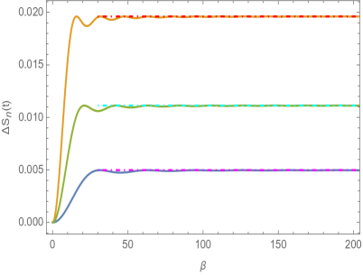
Figure 1: Comparison of exact (solid curves) and approximate expressions for the change in SE with adiabatic approximation, i.e. before the KZ time (dot-dashed lines), for fixed values of $s$ at early times. Dot-dashed lines: magenta ($s=0.1$), cyan ($s=0.15$) and red ($s=0.2$). Solid curves are plotted with the same values $s$ as their associated approximated counterparts.

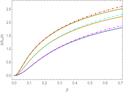
Figure 2: Comparison of exact (solid curves) and approximate expressions (dot-dashed curves) of the change in SE at late times for small $\beta$, with fixed values of $s$. Dot-dashed: magenta ($s=10$), cyan ($s=15$) and red ($s=20$). Solid curves are plotted with the same values $s$ as their associated approximated counterparts.

Case-2. late times and $\beta\ll 1$: In the limit $\beta\ll 1$, and $t\gg\beta$ i.e. $s\gg 1$, expanding the exact expression for $\rho^{2}$ in Eq. (113) and neglecting terms of order $\beta^{2}$ and higher we get KA

$$\rho^{2}(s)\simeq\frac{\eta}{\beta}+\eta\Big{(}s^{2}-\frac{s\pi}{2}+1\Big{)}\beta+\mathcal{O}(1/s)~{}.$$ (116)

The corresponding expression for the change in the SE is therefore given by

$$\Delta S_{n}(t)\sim\frac{1}{2}\ln\Big{(}1+\Big{(}s^{2}-\frac{s\pi}{2}+1\Big{)}\beta^{2}\Big{)}\quad\text{for}\quad\beta\ll 1~{},~{}~{}\text{and}~{}~{}s\gg 1~{}.$$ (117)

In fig - 2, the change in SE is plotted with small $\beta$ and at late times and is compared with the exact expression. It can be seen that for sufficiently small $\beta$, Eq. (117) provides quite a good approximation to the change in SE for different times.

A.2 Cost of the time evolution operator

Next, we compute the cost of the time evolution operator for this frequency profile with the help of the formula derived in section IV and study its various limits. The expression for the time-dependent function $f(t)$, obtained by using the solution of the auxiliary function written above (see Eq. (113)) into Eq. (40), is given in terms of the dimensionless time $s$  by the formula

$$f(s)=\frac{1}{2\beta\eta(1+s^{2})(1+\beta^{2})}\Big{(}(1+2\beta^{2})(1+2\beta^{2}+s^{2})+(s^{2}-1)\cos(\Theta(s))-2s\sqrt{1+\beta^{2}}\sin(\Theta(s))\Big{)}~{},$$ (118)

where we have defined $\Theta(s)=2\sqrt{1+\beta^{2}}\arctan(s)$. Substituting this expression in Eq. (57) we get the expression for the cost. However, this expression is too cumbersome to reproduce here, and therefore we resort to approximate and graphical analysis. To understand the behaviour of the cost function as a function of $s$, first consider its expansion with respect to $s$ around the initial time ($s=0$). This, upto $\mathcal{O}(s^{4})$, can be written as

$$F_{N}^{2}(s)\simeq 4\lambda_{1}^{2}\beta^{2}-8\lambda_{1}^{2}\beta^{2}s^{2}+4\beta^{2}(4\lambda_{1}^{2}+\lambda_{2}^{2})s^{4}+\mathcal{O}(s^{6})~{}.$$ (119)

Here we have written down the expansion of $F_{N}^{2}(s)=\eta^{2}F_{r}^{2}(s)$, instead of just $F_{r}^{2}(s)$, so that the resultant expression is actually independent of $\eta$. In this expansion, only even powers of the dimensionless time parameter $s$ appear, and for small values of it $F_{N}^{2}(s)$ grows quadratically with $\beta$. In fact, as can be easily checked, for $0<s<1$, the cost is always an increasing function of $\beta$. For $s>1$, the behaviour of the cost is more non-trivial. For small values of $\beta$, within the range $0<\beta<1$, irrespective of the value of $s$, the cost grows with $\beta$. While, for $\beta>1$ the nature of the cost depends on the exact value of $s$ as well. Roughly, for large $\beta$, the cost decreases towards zero for large values $s$, while for small values of $s$, the cost, after reaching a minimum value, keeps increasing for large $\beta$. Thus, there is a transition in the behaviour of the cost as we keep increasing $s$ above $1$. These features can be viewed from the plots of $F_{N}^{2}(s)$ shown in Fig. 4, where we have taken $\lambda_{1}^{2}\approx 0.004$ and $\lambda_{2}^{2}\approx 0.05$ for illustration. Note that, even though for the range of $\beta$ shown in this plot, the curve with $s=20$ seems to be decreasing at large $\beta$, it would actually increase for sufficiently large $\beta$. Therefore, unlike the change in the SE, the cost does not saturate to a constant value for large $\beta$, irrespective of the value of $s$.

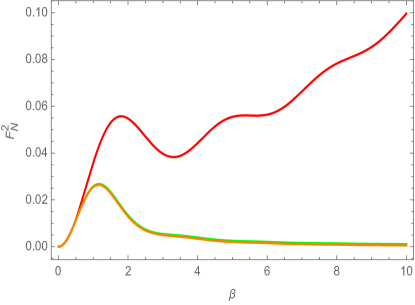
Figure 3: Variation of the cost ($F_{N}^{2}(s)=\eta^{2}F_{r}^{2}(s)$) with respect to $\beta$ for different values of $s$. Here the fixed values of the dimensional time are $s=2$ (red), $s=20$ (green), and $s=200$ (orange).

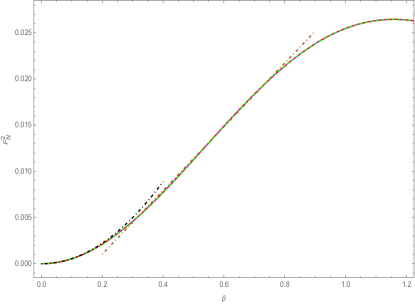
Figure 4: Scaling of the cost ($F_{N}^{2}(s)=\eta^{2}F_{r}^{2}(s)$) at late times for fast quenches. The dashed green curve represents the approximate cost obtained using Eq. (116), while the solid red is the exact one. Quadratic and linear scaling are also shown by dot-dashed black and brown fittings. Here, we have fixed dimensional time $s=200$.

We can obtain a scaling behaviour of the cost at late times ($s\gg 1$) and for $\beta\ll 1$ (i.e., for the case-2 considered for the SE above). Using the expansion of the auxiliary function given in Eq. (116) for late times and small $\beta$, in the expression for the cost, we can obtain an approximate variation of $F_{N}^{2}(s)$ in this limit. This is plotted in Fig. 4 (the dashed green curve), along with the exact expression (red plot), and as can be seen, the truncated expression provides a good approximation for the cost function. Furthermore, in this plot, we have also shown the initial quadratic scaling of the cost for small $\beta$, which later matches with a linear scaling. For the fittings shown in Fig. 4, the numerically obtained equations for the curves are: quadratic scaling $F_{N}^{2}=\beta^{2}/18$ (shown by the dot-dashed black curve), and for linear scaling $F_{N}^{2}=0.0345(\beta-0.17)$ (shown by dot-dashed brown line).

On the other hand, to study the behaviour of the cost at late times, and arbitrary $\beta$, we can expand the cost with respect to $1/s$, keeping $\beta$ fixed, to get the following expression

$$F_{N}^{2}(s)\simeq\frac{\lambda_{1}^{2}+\lambda_{2}^{2}}{(1+\beta^{2})^{2}}\Big{[}1+2\beta^{2}+\cos\Big{(}\pi\sqrt{1+\beta^{2}}\Big{)}\Big{]}^{2}\Big{(}\frac{1}{4\beta^{2}}+\frac{1}{s^{2}}\Big{)}+\mathcal{O}\big{(}\frac{1}{s^{3}}\big{)}~{}.$$ (120)

Therefore, with fixed values of $\beta$, at late times after the quench, the cost always takes constant values, whose magnitude depends on the fixed $\beta$. Also, notice that, at the start of the quench at $s=0$, the cost has the same value as that of a constant frequency HO, as can be seen from the general expression for the cost derived in Eq. (57).

Appendix B Decomposition formula for the time evolution operator of an OTMF

In this appendix we briefly show the derivation of an exact form of the time-evolution operator for an OTMF, and obtain the decomposition formulas by using a $2\times 2$ matrix representation of the generators of the corresponding Lie algebra. We consider the following matrix representation of the $su(1,1)$ Lie algebra generators

$$K_{0}=\frac{1}{2}\left(\begin{array}[]{ccc}-1&0\\ 0&1\end{array}\right)~{},~{}~{}K_{+}=\left(\begin{array}[]{ccc}0&0\\ 1&0\end{array}\right)~{},~{}~{}\text{and}~{}~{}K_{-}=\left(\begin{array}[]{ccc}0&-1\\ 0&0\end{array}\right)~{}.$$ (121)

As can be easily checked, these generators satisfy the commutation relations given in Eq. (91). Using these forms for the generators in the decomposed form for the time evolution operator for an OTMF (see the second expression in Eq. (92)) we obtain an exact matrix representation for it to be of the form

$$\mathcal{U}(t,0)=\exp\Big{[}c_{+}(t)K_{+}\Big{]}\exp\Big{[}c_{0}(t)K_{0}\Big{]}\exp\Big{[}c_{-}(t)K_{-}\Big{]}~{}=\left(\begin{array}[]{ccc}e^{-\frac{c_{0}(t)}{2}}&-c_{-}(t)e^{-\frac{c_{0}(t)}{2}}\\ c_{+}(t)e^{-\frac{c_{0}(t)}{2}}&e^{\frac{c_{0}(t)}{2}}-c_{+}c_{-}e^{-\frac{c_{0}(t)}{2}}\end{array}\right)~{}.$$ (122)

On the other hand, from the first expression for the evolution operator in (92), we can also obtain

$$\mathcal{U}(t,0)=\exp\Big{[}b_{0}(t)K_{0}+b_{+}(t)K_{+}+b_{-}(t)K_{-}\Big{]}~{}=\left(\begin{array}[]{ccc}\cos\chi-\frac{b_{0}}{2\chi}\sin\chi&-\frac{b_{-}}{\chi}\sin\chi\\ \frac{b_{+}}{\chi}\sin\chi&\cos\chi+\frac{b_{0}}{2\chi}\sin\chi\end{array}\right)~{},$$ (123)

where $\chi=(b_{+}b_{-}-\frac{b_{0}^{2}}{4})^{1/2}$ . Comparing these two matrix representations of the time evolution operator, we obtain the relations between two sets of time-dependent coefficients as given in Eq. (93).

References

- (1) M. A. Nielsen, arXiv:quant-ph/0502070 [quant-ph].
- (2) M. A. Nielsen, M. R. Dowling, M. Gu, and A. M. Doherty, Science 311 (2006) 1133.
- (3) M. A. Nielsen and M. R. Dowling, arXiv:quant-ph/0701004 [quant-ph].
- (4) R. Jefferson and R. C. Myers, JHEP 1710, 107 (2017).
- (5) A. Bhattacharyya, A. Shekar, and A. Sinha, JHEP 10, 140 (2018).
- (6) R. Khan, C. Krishnan, and S. Sharma, Phys. Rev. D 98, 126001 (2018).
- (7) L. Hackl and R. C. Myers, JHEP 07 (2018) 139.
- (8) M. Guo, J. Hernandez, R. C. Myers and S. M. Ruan, JHEP 1810, 011 (2018).
- (9) A. Brown, L. Susskind, Phys. Rev. D 100, 046020 (2019).
- (10) E. Caceres, S. Chapman, J. D. Couch, J. P. Hernandez, R. C. Myers and S. M. Ruan, JHEP 03 (2020), 012.
- (11) P. Bueno, J. M. Magan, and C. S. Shahbazi, arXiv:1908.03577 [hep-th].
- (12) H. A. Camargo, P. Caputa, D. Das, M. P. Heller and R. Jefferson, Phys. Rev. Lett. 122 (2019) no.8, 081601.
- (13) T. Ali, A. Bhattacharyya, S.S. Haque, E.H. Kim, and N. Moynihan, JHEP. 04 (2019) 087.
- (14) M. Gautam, N. Jaiswal, A. Gill and T. Sarkar, J. Stat. Mech. 2305 (2023), 053104.
- (15) S. M. Chandran and S. Shankaranarayanan, Phys. Rev. D 107 (2023) no.2, 025003 [arXiv:2205.13338 [hep-th]].
- (16) K. Pal, K. Pal, A. Gill and T. Sarkar, J. Stat. Mech. 2305 (2023), 053108.
- (17) F. Liu, S. Whitsitt, J. B. Curtis, R. Lundgren, P. Titum, Z. C. Yang, J. R. Garrison and A. V. Gorshkov, Phys. Rev. Res. 2, no. 1, 013323 (2020).
- (18) N. Jaiswal, M. Gautam and T. Sarkar, Phys. Rev. E 104, no.2, 024127 (2021).
- (19) Z. Xiong, D.-X. Yao, and Z. Yan, Phys. Rev. B 101, 174305(2020).
- (20) U. Sood, M. Kruczenski, J. Phys. A 55 (2022) 18, 185301 [arXiv- 2106.12648 [quant-ph]].
- (21) N. Jaiswal, M. Gautam and T. Sarkar, J. Stat. Mech. 2207 (2022) no.7, 073105 [arXiv:2110.02099 [quant-ph]].
- (22) K. Pal, K. Pal and T. Sarkar, Phys. Rev. E 105 (2022) no.6, 064117 [arXiv:2106.11842 [quant-ph]].
- (23) S. Roca-Jerat, T. Sancho-Lorente, J. Román-Roche and D. Zueco, SciPost Phys. 15 (2023) no.5, 186.
- (24) W.-H. Huang, arXiv - 2112.13066 [hep-th].
- (25) N. Jaiswal, M. Gautam, A. Gill and T. Sarkar, Eur. Phys. J. B 97 (2024) no.1, 5.
- (26) N. C. Jayarama and V. Svensson, Phys. Rev. B 107 (2023) no.7, 075122.
- (27) V. Balasubramanian, M. Decross, A. Kar and O. Parrikar, JHEP 01 (2020) 134.
- (28) V. Balasubramanian, M. DeCross, A. Kar, Y.C. Li and O. Parrikar,
- (29) S. S. Haque, C. Jana and B. Underwood, Phys. Rev. D 106 (2022) no.6, 063510 [arXiv:2110.08356 [hep-th]].
- (30) L. C. Qu, H. Y. Jiang and Y. X. Liu, JHEP 12 (2022), 065.
- (31) K. Pal, K. Pal and T. Sarkar, Phys. Rev. E 105 (2022) no.6, 064117.
- (32) S. Chowdhury, M. Bojowald and J. Mielczarek, [arXiv:2307.13736 [quant-ph]].
- (33) K. Adhikari, S. Choudhury, S. Kumar, S. Mandal, N. Pandey, A. Roy, S. Sarkar, P. Sarker and S. S. Shariff, Symmetry 15 (2023) no.1, 31 [arXiv:2109.09759 [hep-th]].
- (34) P. Basteiro, J. Erdmenger, P. Fries, F. Goth, I. Matthaiakakis and R. Meyer, Phys. Rev. D 106 (2022) no.6, 065016 [arXiv:2109.01152 [hep-th]].
- (35) G. Camilo and D. Teixeira, Phys. Rev. B 102 (2020) no.17, 174304 [arXiv:2009.00069 [quant-ph]].
- (36) J. Erdmenger, M. Gerbershagen and A. L. Weigel, JHEP 11 (2020), 003 [arXiv:2004.03619 [hep-th]].
- (37) S. Chapman, M. P. Heller, H. Marrochio and F. Pastawski, Phys. Rev. Lett. 120, no. 12, 121602 (2018).
- (38) S. Chapman and G. Policastro, Eur. Phys. J. C 82 (2022) no.2, 128.
- (39) R. Q. Yang, Y. S. An, C. Niu, C. Y. Zhang and K. Y. Kim, Eur. Phys. J. C 79 no.2, 109 (2019).
- (40) R. Q. Yang, Y. S. An, C. Niu, C. Y. Zhang and K. Y. Kim, JHEP 03 (2019) 161.
- (41) R-Q. Yang, K-Y. Kim, JHEP 03 (2019) 010.
- (42) R-Q. Yang, and K-Y.Kim, JHEP 05 (2020) 045.
- (43) H. R. Lewis, W. B. Riesenfeld, J. Math. Phys. 10, 1458, (1968).
- (44) W. Dittrich, M. Reuter, Classical and quantum dynamics, Springer, 2001.
- (45) B. Craps, M. De Clerck, O. Evnin, P. Hacker and M. Pavlov, SciPost Phys. 13 (2022) no.4, 090 [arXiv:2202.13924 [quant-ph]].
- (46) R. Gilmore, Lie Groups, Lie Algebras, and Some of Their Applications, Wiley, 1974.
- (47) L. Frappat, A. Sciarrino, P. Sorba, Dictionary of Lie Algebras and Superalgebras, Academic Press, 2000.
- (48) Y. Weissman, J. Jortner, Phys. Lett. 70A, 177 (1979).
- (49) J. F. Carinena, A. M. Perelomov, M. F. Ranada, M Santander, J. Phys. A: Math. Theor. 41 085301 (2008).
- (50) S. M. Ikhdair, R. Sever, J. Math. Phys. 52, 122108 (2011).
- (51) M.M. Alexandrino and R.G. Bettiol, Lie Groups with Bi-invariant Metrics, Springer International Publishing, (2015).
- (52) A. Davydov, Int J Theor Phys. 50 1451–1467 (2011).
- (53) E. Elizalde, Ten physical applications of spectral zeta functions, Springer, 2012.
- (54) M. Bukov, D. Sels, A. Polkovnikov, Phys. Rev. X 9, 011034 (2019).
- (55) F. Soto-Eguibar, F. A. Asenjo, S. A. Hojman and H. M. Moya-Cessa, arXiv- 2101.05907.
- (56) J. Choi, M.-S. Kim, D. Kim , M. Maamache, S. Menouar, I. Nahme, Ann. Phys. 326 (2011) 1381.
- (57) I. A. Pedrosa, Phys. Rev. A 55, 3219 (1997).
- (58) J. R. Choi, B. H. Kwoen, Int. J. Mod. Phy. B, Vol. 16, No. 31 (2002) 4733–4742.
- (59) P. Caldirola, Nuovo Cimento 18, 393 (1941).
- (60) E. Kanai, Prog. Theor. Phys. 3, 440 (1948).
- (61) G. Dattoli, J. C. Gallardo and A. Torre, Riv. Nuovo Cim. 11N11 (1988), 1-79.
- (62) C. F. Lo, Phys. Rev. A 43, 404 (1991).
- (63) P. G. L. Leach, J. Phys. A: Math. Gen. 16 3261 (1983).
- (64) A. Mostafazadeh, J. Phys. A 31 (1998), 6495-6503 [arXiv:quant-ph/9807002 [quant-ph]].
- (65) M. Ban, J. Opt. Soc. Am. B 10, 1347 (1993).
- (66) J. Anandan and Y. Aharonov, Phys. Rev. Lett. 65, 1697 (1990).
- (67) C Cafaro, S Ray, PM Alsing, Phys. Rev. A 102, 052607 (2020).
- (68) K. Andrzejewski, Quant.Inf.Proc. 21 (2022) 3, 117 [ arXiv:2108.00975].
- (69) G. Di Giulio and E. Tonni, JHEP 05 (2021), 022 [arXiv:2102.02764 [hep-th]].
- (70) S. Ghosh, K. S. Gupta and S. C. L. Srivastava, EPL 120 (2017) no.5, 50005 [arXiv:1709.02202 [quant-ph]].