Gradient Transformation: Towards Efficient and Model-Agnostic Unlearning for Dynamic Graph Neural Networks

Abstract

Graph unlearning has emerged as an essential tool for safeguarding user privacy and mitigating the negative impacts of undesirable data. Meanwhile, the advent of dynamic graph neural networks (DGNNs) marks a significant advancement due to their superior capability in learning from dynamic graphs, which encapsulate spatial-temporal variations in diverse real-world applications (e.g., traffic forecasting). With the increasing prevalence of DGNNs, it becomes imperative to investigate the implementation of dynamic graph unlearning. However, current graph unlearning methodologies are designed for GNNs operating on static graphs and exhibit limitations including their serving in a pre-processing manner and impractical resource demands. Furthermore, the adaptation of these methods to DGNNs presents non-trivial challenges, owing to the distinctive nature of dynamic graphs. To this end, we propose an effective, efficient, model-agnostic, and post-processing method to implement DGNN unlearning. Specifically, we first define the unlearning requests and formulate dynamic graph unlearning in the context of continuous-time dynamic graphs. After conducting a role analysis on the unlearning data, the remaining data, and the target DGNN model, we propose a method called Gradient Transformation and a loss function to map the unlearning request to the desired parameter update. Evaluations on six real-world datasets and state-of-the-art DGNN backbones demonstrate its effectiveness (e.g., limited performance drop even obvious improvement) and efficiency (e.g., at most 7.23$\times$ speed-up) outperformance, and potential advantages in handling future unlearning requests (e.g., at most 32.59$\times$ speed-up).

1 Introduction

To eliminate the impact of target data from the deployed machine learning models, machine unlearning [1, 2] is steadily attracting the attention of academic researchers and industry professionals. It is motivated by practical needs such as (1) compliance with laws for AI governance (e.g., the “right to be forgotten" in GDPR [3]), and (2) removing the adverse effects of identified backdoor or undesired data [4, 5, 6]. Ideally, the model developer could retrain a fresh model on the new data, which is obtained by deleting the unlearning data from the original training data. However, retraining from scratch requires huge source costs (e.g., time and computational source), especially when the model architecture is complex and the training data is on a large scale.

To this end, various methods have been proposed to implement effective and efficient unlearning for independent and identically distributed (IID) data (e.g., tabular or image data) [7]. In the context of graph data, current approaches such as the SISA method (e.g., GraphEraser [8]) and influence function-based methods (e.g., GIF [9], CEU [10]) introduce special designs to deal with the edge between nodes, which breaks the IID assumption in general unlearning methods.

Recently, dynamic graph neural networks (DGNNs) have emerged and been widely deployed due to their impressive learning ability to capture spatial and temporal information included in dynamic graphs [11, 12], which excel in representing complex data in various real-world applications (e.g., traffic networks [13], recommender systems [11]). Nevertheless, to the best of our knowledge, how to perform dynamic graph unlearning has never been explored. Therefore, our research question (RQ) in this paper is “Could we design an effective, efficient, model-agnostic, and post-processing method to implement unlearning for diversified dynamic graph neural networks?” To answer this question, it is not trivial to apply incremental adaptations to the current (static) graph unlearning methods, as the following limitations of these methods and unique challenges exist in dynamic graph unlearning.

Existing Studies. Current unlearning methods for graph data include the SISA method, influence function-based methods, the fine-tuning method, and other methods [7]. (1) For the SISA method [8, 14], it divides the training data into several subsets, each of which is used to train separate submodels. These submodels are then aggregated to deliver services to users. Upon receiving a request for unlearning, the model developer is required to identify the subset that contains the request, remove the data to be unlearned from this subset, and retrain the relevant submodel using the revised subset. (2) For influence function-based methods, it studies how a training sample affects the parameter of a machine learning model [15, 16]. When unlearning requests arise, it calculates the gradient of unlearning samples and the Hessian matrix of the target model to obtain the estimated parameter update for unlearning. (3) For the fine-tuning method (e.g, GraphGuard [6]), it fine-tunes the parameter of the target model by increasing the model loss on the unlearning samples while reducing the loss on the remaining samples, where the model unlearning is achieved by reducing the model accuracy on unlearning samples. (4) In addition to the methods mentioned above, alternative techniques are also applicable for graph unlearning. Specifically, for linear GNNs, the Projector method [17] suggests projecting the model parameters onto a subspace that does not relate to the unlearning sample [17]. In contrast to this model-specific approach, GNNDelete [18] employs a strategy that modifies the architecture by incorporating an additional trainable layer into every layer of the target GNN, which is then trained to achieve the unlearning objectives. Refer to Appendix B.2 for more details on these (static) graph unlearning methods.

Table 1: Comparison between our method and existing methods

Methods	Graph Type	Attributes
		Mod. Agn.	Pos. Pro.	Arc. Inv.
GraphEraser [8]	S
RecEraser [14]	S
GUIDE [19]	S
CGU [20]	S
GIF [9]	S
CEU [10]	S
Projector [17]	S
GNNDelete [18]	S
GraphGuard [6]	S
Ours	D

• In this table, “S” and “D” denotes the static and dynamic graph, respectively.  indicates “Not covered",  indicates “Partially covered",  indicates “Fully covered". “Mod. Agn.", “Pos. Pro”, and “Arc. Inv." indicate “Model-agnostic", “Post-processing”, and “Architecture Invariant", respectively. Refer to Appendix B.2 for more details on the principle and limitations of existing graph unlearning methods.

As shown in Table 1, due to the following limitations of the above static graph unlearning methods, they are not suitable for the unlearning of dynamic graph neural networks (DGNNs). (1) Serving in the pre-processing manner. The SISA method can only be used in the initial development stage. Considering that many DGNNs have been deployed to serve users [21], SISA methods cannot be adapted for post-processing unlearning of these DGNNs, limiting their practicability and applications. (2) Model-specific design. For influence function-based methods, their parameter update estimations are generally established for simple GNN models (e.g., linear GCN model in CEU [10]), whose estimation accuracy is potentially limited due to the complexity and diversity of current state-of-the-art DGNN architectures [22]. Furthermore, these methods are potentially sensitive to the number of GNN layers (e.g., GIF [9]), which further makes these methods dependent on the target model architecture. (3) Unpractical resource requirements. Although influence function-based methods can be used in a post-processing manner, calculations about the Hessian matrix of parameters typically incur high memory costs, particularly when the size of the model parameters is large. For instance, unlearning a state-of-the-art DGNN model named DyGFomer (comprising 4.146 MB floating point parameters) demands a substantial 4.298 TB of storage space, far surpassing the capabilities of common computational (GPU) resources, (4) Changing model architecture. Some methods (e.g., GNNDelete [18]) introduce additional neural layers to target models, which makes them impractical in scenarios where the device space for model deployment is limited (e.g., edge computing devices [23]). (5) Overfitting unlearning samples. The fine-tuning method (e.g., GraphGuard [6]) optimises the parameter of the target model in a post-processing manner. However, the fine-tuning method is prone to overfitting unlearning samples, which potentially harms the model performance on remaining data [24].

Our proposal. To address the limitations of existing methods, we propose a method called Gradient Transformation to implement unlearning of DGNNs. Specifically, we first define the unlearning request and formulate the design goal of dynamic graph unlearning. In this paper, we consider the target DGNN as a tool at hand that natively handles dynamic graph and current model architecture during the unlearning process. For limitations (1) (2) (4) of existing graph unlearning methods, we propose a gradient-based post-processing model to obtain the desired parameter updates w.r.t. unlearning of DGNNs, without changing the architecture of target DGNNs. With specially designed architecture and loss functions, our unlearning paradigm avoids the requiring unpractical resource issue (i.e., limitation (3)) and obviously alleviates the overfitting of fine-tuning methods (i.e., limitation (5)), respectively. Table 1 shows the differences between our method and typical unlearning methods for graph data, and our contributions are as follows.

• For the first time, we study the unlearning problem in the context of dynamic graphs, and formally define the unlearning requests and design goal of dynamic graph neural network unlearning.

• We propose a novel method “Gradient Transformation” with a specialised loss function, which duly handles the intricacies of unlearning requests, remaining data, and DGNNs in the dynamic graph unlearning process.

• We empirically compare our approach with baseline methods on six real-world datasets, evaluation results demonstrate the outperformance of our method in terms of effectiveness and efficiency.

• In addition to the model-agnostic, post-processing, and architecture-invariant characteristics, our learning-based unlearning paradigm potentially highlights a new avenue of graph unlearning study.

2 Preliminaries

Given a time point $t$, a static graph ${G=\{\mathcal{V},\mathcal{E}\}}$ at time $t$ comprises a node set ${\mathcal{V}=\{v_{1},\ldots,v_{|\mathcal{V}|}\}}$ and an edge set ${\mathcal{E}=\{...,(v_{i},v_{j}),...\}}$, which delineates the relational structure among nodes. Generally, a static graph can also be expressed as ${G=(\mathbf{A},\mathbf{X})}$. ${\mathbf{X}\in\mathbb{R}^{|\mathcal{V}|\times d}}$ ($d$ indicates the dimensionality of node features) and ${\mathbf{A}_{i,j}=1}$ if ${e_{ij}=(v_{i},v_{j})\in\mathcal{E}}$, otherwise ${\mathbf{A}_{i,j}=0}$. Due to the need to study the change of graph data over time in some practical scenarios, numerous studies have emerged to explore dynamic graphs and capture their evolving patterns during a time period [25]. Depending on the characterisation manner, dynamic graphs can be categorised into discrete-time dynamic graphs and continuous-time dynamic graphs [21]. In this paper, we focus on continuous-time dynamic graphs. The definition of discrete-time dynamic graphs can be found in the Appendix A.

Continuous-time Dynamic Graphs (CTDG). Given an initial static graph $G_{0}$ and a series of events $\mathcal{O}$, a continuous-time dynamic graph is defined as $S=\{G_{0},\mathcal{O}\}$, where ${\mathcal{O}=[o_{1},...,o_{N}]}$ represents a sequence of observations on graph update events. For example, an event observation sequence with size 3 (i.e., ${N=3}$) could be $\mathcal{O}=[(\textit{add edge},(v_{1},v_{3}),\textit{24-Dec-2023}),$ $(\textit{add node},v_{6},$25-Dec-2023$),$ $(\textit{Feature update},$ $(v_{2},[1,0,1,0]),$ $\textit{25-Dec-2023})]$, where each event $o$ indicates an observation of graph updates. For example, $o_{1}$ indicates that an edge between $v_{1}$ and $v_{3}$ is added to $G_{0}$ on 24-Dec-2023. Note that the symbol $[\cdot]$ in $\mathcal{O}$ indicates that the event order is vital for $S$, as the following dynamic graph neural networks are designed to learn the temporal evolution patterns included in $S$.

Dynamic Graph Neural Networks (DGNNs). For static graphs, various methods (e.g., GCN [26]) have been proposed to capture both node features and graph structures. In addition to these two aspects of information, DGNNs are devised to learn the additional and complex temporal changes in dynamic graphs. For example, in DGNNs [21], the message function designed for an edge event (e.g., (add edge, ($v_{i}$, $v_{j}$), $t$)) could be

$$\mathbf{m}_{i} =msg(\mathbf{s}_{i}(t^{-}),\mathbf{s}_{j}(t^{-}),\Delta t,\mathbf{e}_{i,j}(t)),$$ (1)

$$\mathbf{m}_{j} =msg(\mathbf{s}_{j}(t^{-}),\mathbf{s}_{i}(t^{-}),\Delta t,\mathbf{e}_{i,j}(t)),$$

where $\mathbf{s}_{i}(t^{-})$ represents the latest embedding of $v_{i}$ before time $t$, $\Delta t$ indicates the time lag between current and last events on ($v_{i}$, $v_{j}$), and $\mathbf{e}_{i,j}(t)$ denotes possible edge features in this event. Following this way, various dynamic graph neural networks have been proposed to obtain node representations that capture both spatial and temporal information in dynamic graphs [12].

Tasks on Dynamic Graphs. Two common tasks on dynamic graphs are node classification and link prediction. Generally, given a dynamic graph $S$, a DGNN serve as the encoder to obtain the embedding of nodes, followed by a decoder (e.g., MLP) to complete downstream tasks. Here, we use $f$ to denote the entire neural network that maps a dynamic graph $S$ to the output space desired by the task. In node classification tasks, the parameter $\theta$ of $f$ is trained to predict the label of the nodes at time $t$. In link prediction tasks, $f$ is trained to infer if there is an edge between any two nodes $v_{i}$ and $v_{j}$ at time $t$. Taking the link predictions as an example, the optimal parameter $\theta^{*}$ is obtained by

$$\theta^{*}=\mathcal{A}_{f}(S)=\operatorname{argmin}_{\theta}\ell\left(\mathbf{A}_{t}\mid f_{\theta}(S)\right),$$ (2)

where $\mathcal{A}_{f}$ is the algorithm (e.g., Gradient Descent Method) used to obtain the optimal parameter $\theta^{*}$ of $f$, $\mathbf{A}_{t}$ denotes the true adjacency matrix at time $t$, and $\ell$ represents a loss function (e.g., cross entropy loss). After training from scratch with $\mathcal{A}_{f}$ and $S$ ($t\leq T_{S}$), the $f_{\theta^{*}}$ could be used to make predictions in the future (i.e., $t>T_{S}$), where $T_{S}$ indicates the maximum event time in $S$.

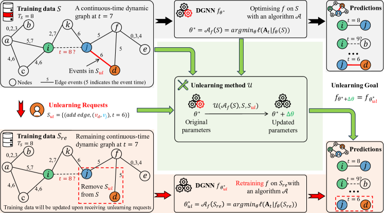
Figure 1: An overview of the unlearning of DGNNs. (1) In the upper half, given a dynamic graph $S$ (maximum event time $T_{S}=8$) and a DGNN $f$, the model developer uses an algorithm $\mathcal{A}_{f}$ to obtain the optimal $f_{\theta^{*}}$, which can make accurate predictions on both training ($t\leq T_{S}$) and test ($t>T_{S}$) data. (2) The lower half illustrates the ideal unlearning process. The left dashed box indicates the change in the training data, and the right dashed box highlights the desired prediction change w.r.t. unlearning. Upon receiving the unlearning request $S_{ul}$, the model developer removes $S_{ul}$ from $S$ and retrains $f$ from scratch to obtain the ideal DGNN $f_{\theta_{ul}^{*}}$. However, retraining from scratch requires huge source costs (e.g., time and computational source). (3) To this end, this paper aims to devise an effective and efficient unlearning method $\mathcal{U}$ to approximate the parameter obtained from retraining, as indicated by the green arrows.

3 Problem Formulation

As shown in Figure 1, a DGNN $f_{\theta^{*}}$ is optimised to learn from its training dataset $S$ ($T_{S}=8$) and then serve users. When a small amount of data $S_{ul}$ ($S_{ul}\subset S$) needs to be removed from the original training dataset (e.g., privacy concerns [1]), unlearning requires that the model $f_{\theta^{*}}$ optimised on $S$ must be updated to forget the knowledge learnt from $S_{ul}$. Specifically, an unlearning method $\mathcal{U}$ aims to update the parameter of $f$ to satisfy

$$\mathtt{dis}(P(\mathcal{U}(\mathcal{A}_{f}(S),S,S_{ul})),P(\mathcal{A}_{f}(S_{re})))=0,$$ (3)

where $\mathtt{dis}(\cdot,\cdot)$ denotes a distance measurement, $P(\cdot)$ indicates the parameter distribution. $\mathcal{A}_{f}(S_{re})$ represents retraining from scratch with the remaining dataset $S_{re}$, where $S_{re}=S\setminus S_{ul}$, $S=S_{re}\cup S_{ul}$, and $S_{re}\cap S_{ul}=\emptyset$.

Unlearning Requests. To clarify the unlearning of DGNNs, here we define the common unlearning requests. Note that the CTDG definition in Section 2 demonstrates the conceptual capability to capture spatial-temporal changes in dynamic graphs [21], while real-world datasets for dynamic link prediction are commonly only composed by adding edge events such as $(\textit{add edge},(v_{1},v_{5}),\textit{26-Dec-2023})$ [27]. Taking into account this fact, we propose the following definition of edge unlearning requests. An edge unlearning request $S_{ul}$ is made up of edge-related events that come from the original training data $S$. For example, $S_{ul}=\{(\textit{add edge},(v_{1},v_{3})$, $\textit{24-Dec-2023}),(\textit{add edge},(v_{1},$ $v_{5}),\textit{26-Dec-2023}),$ $(\textit{add edge},(v_{2},v_{5}),$ $\textit{25-Dec-2023})\}$ requests to forget 3 different “add edge” events. $\{\cdot\}$ suggests that $S_{ul}$ is not sensitive to the order of events, since $S_{ul}$ is only used to indicate which events should be forgotten. Edge unlearning requests are common in real-world applications. For example, a set of users would like to withdraw their negative reviews of some products [28], which have been learnt by the target DGNN $f$ for product recommendations. They can issue edge unlearning requests once their concerns have been addressed.

Remark. Additional types of unlearning request may also occur in DGNNs. For example, $S_{ul}$ is called a node unlearning request if all events in it are related to all activities of specific nodes in the original training dataset $S$. For example, node unlearning requests potentially occur in cases where users arise de-registration or migration requests in a platform (e.g., Reddit [29]), where their historical interactions (i.e., edge events) are expected to be forgotten. Note that, considering that current real-world datasets for dynamic link prediction are commonly only composed of edge events, the above node unlearning request can be transferred into the corresponding unlearning edge events. Additionally, these practical datasets typically consist solely of adding edge events [30]. Hence, this study concentrates on the frequently encountered unlearning requests on adding edge events.

Design Goal. Our objective is to design an unlearning method $\mathcal{U}$ as follows. Given a dynamic graph $S$, a DGNN $f_{\theta^{*}}$ trained on it, and an unlearning request $S_{ul}$, the unlearning method $\mathcal{U}$ takes them as input and outputs the desired parameter update of $f$, i.e., $\Delta\theta=\mathcal{U}_{\varphi}\left(\mathcal{A}_{f}(S),S,S_{ul}\right)$. The $\varphi$ indicates the parameter of $\mathcal{U}$, and it is expected to satisfy

$$\min_{\varphi}\mathtt{dis}(f_{(\theta^{*}+\Delta\theta)},f_{\theta^{*}_{ul}}),$$ (4)

where $\theta^{*}_{ul}=\mathcal{A}_{f}(S_{re})$ indicates the ideal parameter and ${\theta^{*}+\Delta\theta}$ represents the estimated parameter.

4 Gradient Transformation for Unlearning

By analysing $\Delta\theta=\mathcal{U}\left(\mathcal{A}_{f}(S),S,S_{ul}\right)$, we find that the inputs of $\mathcal{U}$ play different roles in the process of unlearning. Generally, $S_{ul}$ issues unlearning requests, $S_{ul}$ and $\mathcal{A}_{f}$ determine the direction of parameter update w.r.t. unlearning. However, directly applying the parameter update derived only from $S_{ul}$ to $f_{\theta^{*}}$ will generally lead to overfitting on $S_{ul}$ and huge performance drops on $S_{re}$. Therefore, $S_{re}$ and $\mathcal{A}_{f}$ work together to improve the direction of parameter update, avoiding the adverse effects of using only $S_{ul}$. This role analysis suggests that a transformation exists which maps the initial gradient to the ultimate parameter updates during the unlearning.

Overview. Given the above intuition, we propose a method called Gradient Transformation to implement dynamic graph unlearning. (1) For the mapping process, we take the initial gradient $\nabla\theta$ w.r.t. $S_{ul}$ as input and transform it with a two-layer MLP-Mixer model to obtain the desired parameter update $\Delta\theta$, i.e., $\mathcal{U}_{\varphi}:\nabla\theta\rightarrow\Delta\theta$. (2) Note that the ideal parameter $\theta^{*}_{ul}$ is not known by $\mathcal{U}_{\varphi}$ in Eq. 4. Thus, we propose a loss function to simulate the desired prediction behaviours of an ideal model $f_{\theta^{*}_{ul}}$.

Gradient Transformation model. Given a dynamic graph $S$, the optimal parameter $\theta^{*}$ of a dynamic graph neural network $f$ is obtained by solving $\theta^{*}=\operatorname{argmin}_{\theta}\ell\left(Y\mid f_{\theta}(S)\right)$. As shown in Figure 2, after receiving unlearning requests $S_{ul}$, we first calculate the corresponding gradient $\nabla\theta$ w.r.t. the desired unlearning goal. Specifically,

$$\nabla\theta=\frac{d}{d\theta}\ell(\widehat{Y_{ul}}\mid f_{\theta^{*}},S_{ul}),$$ (5)

where $\widehat{Y_{ul}}$ indicates the desired prediction results on the unlearning samples $S_{ul}$. For example, in the context of link prediction tasks and given $S_{ul}=\{o_{1},...,o_{n}\}$ consists of “add edge” events, the initial gradient information is obtained by ${\nabla\theta=\frac{d}{d\theta}\sum_{o\in S_{ul}}\ell(\mathbf{A}_{t;i,j}=0\mid f_{\theta^{*}})}$, where $i$, $j$ and $t$ represent the nodes and time involved in the event $o=(\textit{add edge},$ $(v_{i},v_{j}),t)$. ${\mathbf{A}_{t;i,j}=0}$ indicates that $f$, which predicts $\mathbf{A}_{t;i,j}=1$, is expected to forget the existence of $S_{ul}$ in its original training data $S$.

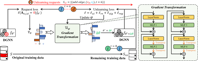
Figure 2: The overview of our Gradient Transformation method.

Given the initial gradient $\nabla\theta$, our gradient transformation model $\mathcal{U}$ takes it as input and outputs the desired parameter update $\Delta\theta$ of the target model $f$. Combined with the original parameter $\theta^{*}$, the updated parameter is obtained by applying $\theta^{*}+\Delta\theta=\theta^{*}+\mathcal{U}(\Delta\theta)$, where $f_{\theta^{*}+\Delta\theta}$ is expected to behave the same as $f_{\theta^{*}_{ul}}$. In this paper, we use a two-layer MLP-Mixer to serve as the unlearning model $\mathcal{U}$. As shown in Figure 2, given the initial gradient as input (i.e., $\nabla\theta\rightarrow\mathbf{H}_{\mathtt{in}}$), the operation of $\mathcal{U}$ is presented as follows

$$\mathbf{H}_{\mathtt{tok}}^{(1)} =\mathbf{H}_{\mathtt{in}}+\mathbf{W}_{\mathtt{tok}}^{(2)}\mathtt{GeLU}\left(\mathbf{W}_{\mathtt{tok}}^{(1)}\mathtt{LN}(\mathbf{H}_{\mathtt{in}})\right),\mathbf{H}_{\mathtt{cha}}^{(1)}=\mathbf{H}_{\mathtt{tok}}^{(1)}+\mathtt{GeLU}\left(\mathtt{LN}(\mathbf{H}_{\mathtt{tok}}^{(1)})\mathbf{W}_{\mathtt{cha}}^{(1)}\right)\mathbf{W}_{\mathtt{cha}}^{(2)},$$ (6)

$$\mathbf{H}_{\mathtt{tok}}^{(2)} =\mathbf{H}_{\mathtt{cha}}^{(1)}+\mathbf{W}_{\mathtt{tok}}^{(4)}\mathtt{GeLU}\left(\mathbf{W}_{\mathtt{tok}}^{(3)}\mathtt{LN}(\mathbf{H}_{\mathtt{cha}}^{(1)})\right),\mathbf{H}_{\mathtt{cha}}^{(2)}=\mathbf{H}_{\mathtt{tok}}^{(2)}+\mathtt{GeLU}\left(\mathtt{LN}(\mathbf{H}_{\mathtt{tok}}^{(2)})\mathbf{W}_{\mathtt{cha}}^{(3)}\right)\mathbf{W}_{\mathtt{cha}}^{(4)},$$

where $\mathtt{GeLU}$ indicates the active function and $\mathtt{LN}$ denotes the layer normalisation. With $\Delta\theta=\mathcal{U}(\Delta\theta)$ (i.e., $\mathbf{H}_{\mathtt{cha}}^{(2)}\rightarrow\Delta\theta$), we obtain the unlearned target model $f_{\theta^{*}+\Delta\theta}$. In this paper, all parameters of Eq. (6) are denoted as $\varphi$, and $\mathcal{U}_{\varphi}$ is optimised by the following loss function.

Unlearning Loss Function. Unlearning $S_{ul}$ has the following potential impacts on DGNN $f_{\theta^{*}}$, and the corresponding loss functions describe the desired behaviours of $f_{\theta^{*}_{ul}}$.
(1) Changed predictions on invariant representations. An event $o_{i}$ in $S_{ul}$ could have observed a series of events that remained in $S_{re}$ before its occurrence time, while the unlearning expects $f$ to predict differently on the same representations. Therefore, the unlearning loss is defined as

$$\ell_{ul}=\ell(\widehat{Y_{ul}}\mid f_{\theta^{*}+\Delta\theta},S_{ul}),$$ (7)

(2) Invariant predictions on changed representations. For an even $o\in S_{re}$, its involved nodes may have different representations because their neighbours are potentially different before and after removing $S_{ul}$, while it requires $f$ to make unchanged predictions (as shown by $(v_{i},v_{j})$ at $t=8$ in Figure 4). Thus, the performance loss for $S_{re}$ is defined as

$$\ell_{re}=\ell(Y_{re}\mid f_{\theta^{*}+\Delta\theta},S_{re}),$$ (8)

(3) Avoiding the performance drop caused by unlearning. Due to the data-driven nature of current machine learning methods, the size deduction of $S$ caused by the removal of unlearning data $S_{ul}$ could potentially harm the performance of $f$ on the test data $S_{te}$. Considering that $l_{re}$ is focused on maintaining model performance in training data $S_{re}$, we propose another loss to improve generalisability of $f$ in test data $S_{te}$ as

$$\ell_{reg}=d(Y_{re},Y_{val})=||\mathbb{E}(Y_{re})-\mathbb{E}(Y_{val})||_{2}+\sum_{i=2}^{k}||\mathbb{E}(Y_{re}-\mathbb{E}(Y_{re}))^{i}-\mathbb{E}(Y_{val}-\mathbb{E}(Y_{val}))^{i}||_{2}$$ (9)

where $Y_{re}$ and $Y_{val}$ indicate the predictions of $f_{\theta^{*}+\Delta\theta}$ on $S_{re}$ and validation dataset $S_{val}$, respectively. $d$ indicates the central moment discrepancy function [31] that measures the distribution difference.
(4) Avoiding the overfitting caused by unlearning. Due to the ResNet-like design of Gradient Transformation, our method $\mathcal{U}_{\varphi}$ may be prone to overfit $S_{ul}$ w.r.t. its desired label $\widehat{Y_{ul}}$. Although this behaviour is desired by unlearning requests, it potentially harms the generalisation ability of $f$ on $S_{ul}$, i.e., the $f$ retrained on $S_{re}$ could perform/generalise well on $S_{ul}$ due to its knowledge learnt from $S_{re}$. Refer to Appendix D for examples. To avoid this potential adverse effect, a generalisation regularisation w.r.t. unlearning is defined as

$$\ell_{ulg}=d(\widehat{Y_{ul}},Y_{ul}^{c})$$ (10)

where $\widehat{Y_{ul}}$ denotes the desired predictions on $S_{ul}$, and $Y_{ul}^{c}$ indicates the prediction of $f_{\theta^{*}+\Delta\theta}$ on the counterpart of $S_{ul}$, which could be any event related to nodes in $S_{ul}$ (e.g., $v_{d}$ or $v_{j}$) that does not occur at $t=6$ (e.g., $S_{ul}^{c}=\{(\textit{add edge},(v_{d},v_{e}),t=6),(\textit{add edge},(v_{j},v_{e}),t=6)\}$).

In this paper, our unlearning method Gradient Transformation $\mathcal{U}_{\varphi}$ is trained by the following loss

$$\ell=\ell_{re}+\alpha\ell_{reg}+\beta\ell_{ul}+\gamma\ell_{ulg}$$ (11)

Discussions. (1) Our method can be used in a post-processing and model-agnostic manner to implement DGNN unlearning. It is independent of one specific architecture (e.g., Transformer-based model DyGFormer [30]) and maintains the invariant architecture of target DGNN models, which overcomes the model-specific and changing architecture limitations of current methods for (static) graph unlearning. (2) For resource concern, the influence function-based methods ask for $O(n^{2})$ space to store the Hessian matrix, where $n$ denotes the parameter number of target models. In contrast, the space requirement of our method is $O(nd_{W})$, where $d_{W}$ indicates the average embedding dimension in Eq. (6) and $d_{W}<<n$. Although this design greatly reduces the resource requirement of our method, it potentially faces a resource bottleneck when handling large DGNN models in the future, which will be the future work of this paper. (3) Note that, with the aim of unlearning DGNNs, this paper is motivated to address the limitations of exiting static graph unlearning methods. Although the model-agnostic advantage enables its potential in unlearning other models (e.g., models for static graphs or images), this paper focusses on dynamic graph neural networks for link predictions.

5 Experiments

5.1 Experimental Setup

Datasets, DGNNs, and Unlearning Requests. We evaluated our method on six commonly used datasets for dynamic link prediction [27], including Wikipedia, Reddit, MOOC, LastFM [11], UCI [32], and Enron [33]. We use two state-of-the-art DGNNs, i.e., DyGFormer [30] and GraphMixer [34], as the backbone models in our evaluations (See Appendix E for more details). For data partition and DGNN training, we followed previous work DyGLib [30]. In our evaluations, we set $k=2$ in the moment discrepancy function (see Eq. (9) and (10)). The channel/token dimension (i.e., Eq. (6)) is set to 32. For the loss function (11), we set $\alpha=1.0$, $\beta=0.1$, and $\gamma=0.1$. For the generation of unlearning data, we first randomly sample a fixed number of events as anchor events and use their historically observed events (e.g., 621445 events in (LastFM, DyGFormer)) as unlearning data $S_{ul}$. For each (dataset, DGNN) combination, we ran five times on RTX 3090 GPUs to obtain the evaluation results. More details about experiments can be found in our code.
Baselines. In this paper, we focus on evaluating post-processing and model-agnostic unlearning methods for dynamic graph neural networks. Baseline methods include retraining, fine-tuning, and fine-tuning only with unlearning requests. Also, we use retraining from scratch as the gold standard to evaluate unlearning methods. As a typical post-processing method, the fine-tuning method uses the loss $\ell_{re}+\ell_{ul}$ to update the DGNN parameters. To evaluate how overfitting a model will be when only using unlearning requests, we use a variant of fine-tuning that only uses $\ell_{ul}$. Note that current SISA and influence function-based methods are not suitable as baselines for DGNNs. This is because the former is designed as a pre-processing method, while the resource-intensive issue of the latter invalidates its practicability in the unlearning of DGNNs. Refer to Section B.2 for more details.
Metrics. We use the retrained model as the criterion, and the unlearned model $f_{(\theta^{*}+\Delta\theta)}$ is expected to perform similarly to or better than $f_{\theta^{*}_{ul}}$. Specifically, the evaluation of an unlearning method includes three different aspects of metrics, i.e., model effectiveness, unlearning effectiveness, and unlearning efficiency.

(1) Model Effectiveness. A DGNN $f$ is trained to serve its users in downstream tasks, where its performance is vital during its inference period. In this paper, we use $\Delta\mathtt{AUC}(S_{te})=\mathtt{AUC}(Y,f_{\theta^{*}+\Delta\theta}(S_{te}))-\mathtt{AUC}(Y,f_{\theta^{*}_{ul}}(S_{te}))$ as the metric, where $S_{te}$ represents the test dataset and $\mathtt{AUC}$ indicates the numeric value of the area under the ROC curve (AUC). A higher $\Delta\mathtt{AUC}(S_{te})$ indicates a better unlearning method. Similarly, we also use $\Delta\mathtt{Acc}(S_{re})$ to evaluate unlearning methods w.r.t. model performance on the remaining data $S_{re}$, where $\mathtt{Acc}$ indicates the accuracy function.
(2) Unlearning Effectiveness. According to the data-driven nature of DGNNs, a well-retrained model $f_{\theta^{*}_{ul}}$ could generalise well on unseen samples (e.g. $S_{ul}$) because it has learnt knowledge from $S_{re}$ and the same data patterns potentially exist in both $S_{re}$ and $S_{ul}$. Therefore, this paper uses $|\Delta\mathtt{Acc}(S_{ul})|$ to evaluate the effectiveness of unlearning. A lower value indicates a better unlearning method.
(3) Unlearning Efficiency. We compare the average time cost $\mathtt{t}_{ave}$ (seconds) and the degree of speed-up of different methods to evaluate their efficiency.

5.2 Model Performance on test data ${S_{te}}$

Table 2: $\mathtt{AUC}(S_{te})$ comparison between our method and baseline methods ($\Delta\mathtt{AUC}(S_{te})\uparrow$).

[flushleft] Methods Retraining Fine-tuning-ul Fine-tuning Ours Datasets DyGFormer Wikipedia 0.9862 ± 0.0004 0.8491 ± 0.1855 0.9542 ± 0.0334 0.9859 ± 0.0004 UCI 0.9422 ± 0.0005 0.7855 ± 0.2867 0.7850 ± 0.2864 0.9396 ± 0.0020 Reddit 0.9885 ± 0.0006 0.6459 ± 0.1049 0.9479 ± 0.0068 0.9902 ± 0.0001 MOOC 0.7477 ± 0.0289 0.5342 ± 0.0986 0.7949 ± 0.0275 0.8509 ± 0.0032 LastFM 0.8675 ± 0.0154 0.4409 ± 0.0967 0.5846 ± 0.0679 0.7953 ± 0.0523 Enron 0.8709 ± 0.0312 0.3109 ± 0.1018 0.8240 ± 0.0568 0.8452 ± 0.0867 Datasets GraphMixer Wikipedia 0.9632 ± 0.0017 0.9576 ± 0.0032 0.9578 ± 0.0031 0.9683 ± 0.0016 UCI 0.9089 ± 0.0052 0.9174 ± 0.0072 0.9182 ± 0.0068 0.9149 ± 0.0069 Reddit 0.9650 ± 0.0001 0.9434 ± 0.0093 0.9444 ± 0.0086 0.9717 ± 0.0004 MOOC 0.8257 ± 0.0060 0.8179 ± 0.0062 0.8179 ± 0.0062 0.8367 ± 0.0056 LastFM 0.7381 ± 0.0020 0.7304 ± 0.0011 0.7304 ± 0.0011 0.7358 ± 0.0014 Enron 0.8462 ± 0.0009 0.8495 ± 0.0035 0.8495 ± 0.0035 0.8490 ± 0.0036

• In this table, the values indicate the average and variance results of five runs, and the results with largest $\Delta\mathtt{AUC}(S_{te})$ among Fine-tuning-ul, Fine-tuning, and our method is highlighted in bold.

As the prediction quality is vital for DGNNs in serving users, we first evaluate their performance on $S_{te}$. Table 2 confirms the outperformance of our method w.r.t. $\Delta\mathtt{AUC}(S_{te})\uparrow$. Moreover, we have the following observations. (1) Due to the complex Transformer-based design, the retrained DyGFormer outperforms other backbone models in most cases, which is consistent with previous research [30]. (2) Among all unlearning methods, the fine-tuning-ul only uses the unlearning loss $\ell_{ul}$ (see Eq. (7)) to obtain the target DGNN parameters, which harms their performance in test data $S_{te}$. For example, with the DyGFormer, the average $\mathtt{AUC}$ score on the Enron dataset is only 0.3109, which is extremely below that of retraining, i.e., 0.8709. This observation indicates that it is vital to take into account the remaining training data $S_{re}$ to reduce the performance cost of unlearning methods. (3) As an integrated version, the fine-tuning method performs better on the test data $S_{te}$ than the fine-tuning-ul method due to the use $\ell_{re}+\ell_{ul}$ as the loss in optimising model parameters. However, the performance compromise still exists in most cases. (4) Note that even in the cases where our method is not the best, it still has competitive performance. This can be attributed to $\ell_{reg}=d(Y_{re},Y_{val})$ in the loss function, which helps $f$ generalise well on the test data $S_{te}$.

Table 3: $\mathtt{Acc}$ comparison between our method and baseline methods.

[flushleft] Datasets Methods DyGFormer GraphMixer $\mathtt{Acc}(S_{re})/\Delta\mathtt{Acc}\uparrow$ $\mathtt{Acc}(S_{ul})/|\Delta\mathtt{Acc}|\downarrow$ $\mathtt{Acc}(S_{re})/\Delta\mathtt{Acc}\uparrow$ $\mathtt{Acc}(S_{ul})/|\Delta\mathtt{Acc}|\downarrow$ Wikipedia Retraining 0.9507 ± 0.0004 0.1470 ± 0.0435 0.9105 ± 0.0028 0.2050 ± 0.0078 Fine-tuning-ul 0.7541 ± 0.1463 0.1574 ± 0.1005 0.9112 ± 0.0056 0.1666 ± 0.0146 Fine-tuning 0.9062 ± 0.0545 0.3962 ± 0.0797 0.9117 ± 0.0056 0.1640 ± 0.0111 Ours 0.9529 ± 0.0008 0.1773 ± 0.0330 0.9307 ± 0.0016 0.1339 ± 0.0145 UCI Retraining 0.8458 ± 0.0008 0.2056 ± 0.0097 0.8685 ± 0.0003 0.1361 ± 0.0080 Fine-tuning-ul 0.7552 ± 0.1427 0.3850 ± 0.3515 0.8705 ± 0.0036 0.1246 ± 0.0066 Fine-tuning 0.7572 ± 0.1437 0.4006 ± 0.3408 0.8710 ± 0.0034 0.1235 ± 0.0080 Ours 0.8484 ± 0.0020 0.2057 ± 0.0028 0.8737 ± 0.0019 0.1258 ± 0.0055 Reddit Retraining 0.9460 ± 0.0012 0.0540 ± 0.0033 0.9009 ± 0.0003 0.0477 ± 0.0028 Fine-tuning-ul 0.6665 ± 0.0817 0.3116 ± 0.2221 0.8874 ± 0.0058 0.3361 ± 0.0512 Fine-tuning 0.8592 ± 0.0104 0.2433 ± 0.0727 0.8879 ± 0.0060 0.3342 ± 0.0516 Ours 0.9487 ± 0.0006 0.0476 ± 0.0014 0.9326 ± 0.0005 0.0212 ± 0.0021 MOOC Retraining 0.8176 ± 0.0124 0.0452 ± 0.0389 0.8171 ± 0.0033 0.1240 ± 0.0068 Fine-tuning-ul 0.6090 ± 0.1116 0.4962 ± 0.3865 0.8161 ± 0.0053 0.0552 ± 0.0110 Fine-tuning 0.7510 ± 0.0252 0.4804 ± 0.0595 0.8161 ± 0.0053 0.0552 ± 0.0110 Ours 0.7950 ± 0.0036 0.0472 ± 0.0164 0.8222 ± 0.0026 0.0630 ± 0.0130 LastFM Retraining 0.8738 ± 0.0049 0.3110 ± 0.1099 0.6583 ± 0.0006 0.2918 ± 0.0075 Fine-tuning-ul 0.5578 ± 0.0660 0.5322 ± 0.2697 0.6593 ± 0.0024 0.3059 ± 0.0071 Fine-tuning 0.7590 ± 0.0163 0.9103 ± 0.0232 0.6597 ± 0.0024 0.2980 ± 0.0030 Ours 0.8198 ± 0.0224 0.2834 ± 0.1714 0.6632 ± 0.0015 0.3009 ± 0.0080 Enron Retraining 0.9321 ± 0.0119 0.2101 ± 0.0399 0.8007 ± 0.0009 0.2866 ± 0.0215 Fine-tuning-ul 0.5012 ± 0.0007 0.9953 ± 0.0059 0.8109 ± 0.0015 0.2938 ± 0.0569 Fine-tuning 0.9015 ± 0.0329 0.2759 ± 0.1047 0.8110 ± 0.0015 0.2771 ± 0.0498 Ours 0.8226 ± 0.1652 0.2324 ± 0.2934 0.8100 ± 0.0012 0.2944 ± 0.0341

• $\mathtt{Acc}(S_{re})$ results represent the model performance on remaining training data, and the results (excluding the retraining method) with largest $\Delta\mathtt{Acc}$ is highlighted in bold. $\mathtt{Acc}(S_{ul})$ results indicate the model performance on unlearning data, and the results with the smallest $|\Delta\mathtt{Acc}|$ are highlighted in bold. Underline points out the result where there is an extreme overfitting on $S_{ul}$.

5.3 Model Performance on remaining data ${S_{re}}$ and unlearning data ${S_{ul}}$

Table 3 showcases the prediction accuracy comparison among unlearning methods on $S_{re}$ and $S_{ul}$. Specifically, (1) although baselines are potentially at the cost of the model performance, our method still generally performs better in the remaining training dataset $S_{re}$ w.r.t. $\mathtt{Acc}(S_{re})\uparrow$. For example, for DyGFormer on the Reddit dataset, the $\Delta\mathtt{Acc}$ of the fine-tuning method is $-0.0868$ while our method still maintains the same level of prediction performance (i.e., $\Delta\mathtt{Acc}=+0.0017$). (2) For the unlearning request $S_{ul}$, a retrained model can still predict well on unseen samples $S_{ul}$ due to its generalisation ability. However, as indicated by the underline results, when comparing with the retraining method, we observed that the fine-tuning and fine-tuning-ul methods have extreme overfitting to $S_{ul}$. In contrast, our method performs similarly to the retraining method w.r.t. $|\Delta\mathtt{Acc}(S_{ul})|\downarrow$, which highlights the outperformance of our method in approximating unlearning.

5.4 Unlearning Efficiency

Figure 3 demonstrates the time cost of different methods to implement unlearning on the Wikipedia dataset. We observe that (1) Due to the use of additional $S_{re}$ in the unlearning process, the fine-tuning method is generally slower than the fine-tuning-ul method. (2) Although the baselines are able to make the unlearning process efficient, the overfitting on $S_{ul}$ limits their speed to obtain their optimal solutions, where it is not trivial to navigate between the unlearning effectiveness and model performance. On the contrary, our method is always more efficient than all other baselines. The time cost on other datasets can be found in Figure 6.

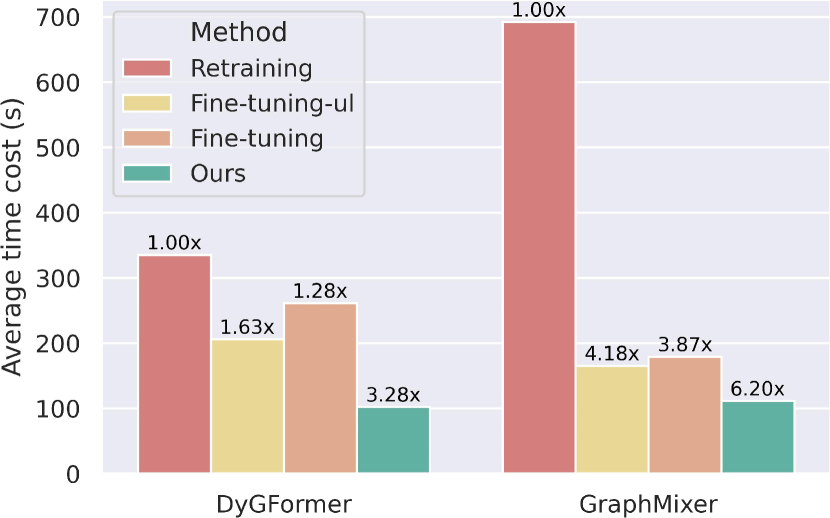
Figure 3: Time cost ($\mathtt{t}_{ave}$) comparison on the Wikipedia dataset. The numerical values on the bars (e.g., $6.20\times$) indicate the degree of acceleration relative to the retraining approach.

5.5 Other Evaluations

Membership Inference. We conducted membership inference evaluations to evaluate the extent of unlearning. Evaluation results indicate that our method achieves an average unlearning rate $81.33\%$ on the test data (See Appendix F.1).

Independent of DGNN Architecture. As shown in Table 5, we further verify that our method is independent of the DGNN architecture by evaluating it on the CAWN model [35], whose random walking-based architecture is different from that of DyGFormer and GraphMixer.

Potential Benefits. The learning nature of our method brings potential benefits when handling future unlearning requests. Using the gradient of new unlearning requests as input, our method could directly output the desired parameter update. Table 6 shows that our method obtains almost the same unlearning results as the retraining method. For example, besides performance increments, the largest $|\Delta\mathtt{Acc}(S_{ul})|$ is only 0.0208 while the speed-up is at least 25$\times$. However, this benefit of our method could be limited due to the complex relationships between $S_{re}$ and $S_{ul}$ and the lack of ground truth $\Delta\theta$ in the training of our method. In cases where the benefit is limited, model developers can rerun our method in Figure 2 to conduct future unlearning.

6 Conclusion

In this paper, we study dynamic graph unlearning and propose a method called Gradient Transformation, which is effective, efficient, model-agnostic, and can be used in a post-processing manner. Empirical evaluations on real-world datasets confirm the effectiveness and efficiency outperformance of our method, and we also demonstrate its potential advantages in handling future unlearning requests. In our future research, we plan to investigate the causal relationships between events from the perspective of unlearning, while also delving into the intricate interplay between the remaining data and the unlearning data.

Appendix A Concepts

Discrete-time Dynamic Graphs (DTDG). Given a benign sequence of static graphs with time length ${T=t-1}$, a discrete-time dynamic graph is denoted as $S=\{G_{1},G_{2},\ldots,G_{t-1}\}$, where ${G_{k}=\{\mathcal{V}_{k},\mathcal{E}_{k}\}}$ denotes the $k$-th snapshot of a dynamic graph. In the form of ${G_{k}=(\mathbf{A}_{k},\mathbf{X}_{k})}$, ${\mathbf{A}_{k;i,j}=1}$ if there is a link from $v_{i}$ pointing to $v_{j}$ in the $k$-th snapshot, otherwise ${\mathbf{A}_{k;i,j}=0}$; $\mathbf{X}_{k;i}$ represents the node feature of $v_{i}$ in $G_{k}$, and $\mathbf{X}_{k;i,j}$ indicates its $j$-th feature value. Thus, a discrete-time dynamic graph can also be depicted as ${S=\{(\mathbf{A}_{1},\mathbf{X}_{1}),(\mathbf{A}_{2},\mathbf{X}_{2}),\ldots,(\mathbf{A}_{t-1},\mathbf{X}_{t-1})\}}$.

Appendix B Related Work

B.1 Dynamic Graph Neural Networks

The dynamic graph is a powerful data structure that depicts both spatial interactions and temporal changes in practical data from various real-world applications (e.g., traffic prediction [36]). Dynamic graph neural networks (DGNNs) are proposed to learn the complex spatial-temporal patterns in these data [25, 12, 37]. Next, we will present some representative methods to introduce how dynamic graph neural networks learn from dynamic graphs.

Depending on the type of dynamic graph (as shown in Section 2), current methods can be categorised into DGNNs for discrete-time and continuous-time dynamic graphs [30].
(1) For discrete-time methods, they generally employ a GNN model for static graphs to learn spatial representations and an additional module (e.g., RNN [38]) to capture the temporal changes of the same node in different static snapshot graphs. In this paper, we focus on DGNNs designed for continuous-time dynamic graphs. Unlike discrete-time dynamic graphs, this type of data naturally records dynamic changes (i.e., fine-grained order of different changes) without determining the time interval among the snapshots in discrete-time dynamic graphs [39]
(2) Some typical continuous-time methods are RNN-based models (e.g., JODIE [11]), temporal point process models (e.g., DyRep [40]), time embedding-based models (e.g., TGAT [39], TGN [41]), and temporal random walk methods [35, 12].

B.2 Unlearning Methods

Retraining. Intuitively, for the target model to be unlearned, deleting the unlearning data from the original training data and retraining from scratch will directly meet the requirement from the perspective of unlearning. However, retraining from scratch comes at the cost of huge time and computational resources, given large-scale training data or complex model architectures. To this end, various methods have been proposed to satisfy the efficiency requirement of unlearning. Current methods designed for GNNs focus on static graph unlearning, including SISA methods, influence function methods, and other approaches.

SISA Methods. Referring to “Sharded, Isolated, Sliced, and Aggregated”, the SISA method represents a type of ensemble learning method and is not sensitive to the architecture of target models (i.e., model-agnostic). Specifically, SISA first divides the original training data $\mathcal{D}_{o}$ into $k$ different and disjoint shard datasets, i.e., $\mathcal{D}_{o}^{1},...,\mathcal{D}_{o}^{k}$, which are used to train $k$ different submodels $f^{1},...,f^{k}$ separately. To obtain the final prediction on a sample $v_{i}$, SISA aggregates $f^{1}(v_{i}),...,f^{k}(v_{i})$ together to obtain a global prediction. Upon receiving the unlearning request for a sample $v_{j}$, SISA first removes $v_{j}$ from the shard $\mathcal{D}_{o}^{j}$ that includes it and only retrains $f^{j}$ to obtain the updated model, which significantly reduces the time cost compared with retraining the whole model from scratch on $\mathcal{D}_{o}\setminus v_{j}$ (i.e., the dataset with removing $v_{j}$).

Typical methods. The SISA method divides the training dataset into several subsets and trains submodels on them, followed by assembling these submodels to serve users. In the context of graph unlearning, it is not trivial to directly split a whole graph into several subgraphs, as imbalanced partition (e.g., imbalance of node class) potentially leads to decreased model performance. To this end, GraphEraser [8] and RecEraser [14] propose balanced graph partition frameworks and learning-based aggregation methods. Unlike the transductive setting of GraphEraser, Wang et al. [19] propose a method called GUIDE in the inductive learning setting, which takes the fair and balanced graph partitioning into consideration.

Limitations. The weakness of SISA methods mainly includes the following two aspects.
(1) Efficacy Issue on A Group of Unlearning Requests. The SISA method faces the efficiency issue when dealing with a group/batch of unlearning requests. Note that the efficiency of SISA methods in facilitating unlearning stems from the fact that retraining a single submodel is more efficient than retraining the entire model that was trained on the whole dataset, which is suitable for implementing unlearning of a single sample. However, the SISA method will have to retrain all submodels when a group of unlearning requests binds to all shards, limiting its unlearning efficiency capacity.
(2) Serving in A Pre-processing Manner. Note that SISA methods can only be used in the initial phase of model development. Once the machine learning models are deployed, the current SISA methodology cannot implement unlearning on them in a post-processing manner.

Influence Function based Methods. Current research on the influence function studies how a training sample impacts the learning of a machine learning model [15, 16]. Generally, given a model $f$, its optimal parameter is obtained by ${\theta^{*}=\operatorname{argmin}_{\theta}\sum_{v\in\mathcal{D}_{o}}\ell\left(f_{\theta}\mid\mathcal{D}_{o}\right)}$, where $\ell$ indicates a convex and twice-differential loss function. For the unleraning request on a training sample $v_{j}$, the desired model parameter $\theta^{*}_{ul}$ is defined as ${\theta^{*}_{ul}=\operatorname{argmin}_{\theta}\sum_{v\in\mathcal{D}_{o}\setminus v_{j}}\ell\left(f_{\theta}\mid{\mathcal{D}_{o}\setminus v_{j}}\right)}$. Without retraining $f$, current influence function-based methods are designed to estimate the parameter change $\Delta\theta$ and use it to approximate $\theta^{*}_{ul}$ (i.e., ${\theta^{*}_{ul}\approx\theta^{*}+\Delta\theta}$). The estimation can be obtained by ${\Delta\theta=\mathbf{H}^{-1}_{\theta^{*}}\nabla_{\theta^{*}}\ell\left(f_{\theta}\mid v_{j}\right)}$, where ${\mathbf{H}^{-1}_{\theta^{*}}=\sum_{v\in\mathcal{D}_{o}}\nabla_{\theta^{*}}^{2}\ell\left(f_{\theta}\mid\mathcal{D}_{o}\right)}$ denotes the Hessian matrix.

Typical methods. Current research on the influence function studies how a training sample affects the learning of a machine learning model [15, 16]. In the context of graph unlearning, the influence function is more complex since the edges between nodes break the independent and identically distributed assumption of training samples in the above formulations. Therefore, the multi-hop neighbours of an unlearning node or nodes involved in an unlearning edge have been considered to correct the above estimation of $\Delta\theta$, and more details can be found in recent works called Certified Graph Unlearning (CGU) [20], GIF [9], CEU [10], and an unlearning method based on Graph Scattering Transform (GST) [42]. Note that these methods generally rely on the static graph structure to determine the scope of nodes that need to be involved in the final influence function, which cannot be directly adapted to dynamic graphs.

Limitations. The weakness of influence function-based methods mainly includes the following two aspects.
(1) Model-specific design. Current estimations of $\Delta\theta$ in graph unlearning are generally established on simple GNN models (e.g., linear GCN model in CEU [10]), whose estimation accuracy is potentially limited due to the complexity and diversity of current state-of-the-art GNN architectures (e.g., Graph Transformer Networks [22]). Furthermore, these methods are not strictly model-agnostic, since they need access to the architecture of target models (e.g., layer information) to determine the final influence function (e.g., GIF [9]), that is, they are sensitive to GNN layers.
(2) Resource intensive. Although influence function-based methods can be used in a post-processing manner, the calculation of the inverse of a Hessian matrix (i.e., $\mathbf{H}^{-1}_{\theta^{*}}$) generally has a high time complexity and memory cost when the model parameter size is large. For example, for a DyGFormer model [30] with single precision floating point format parameters, it requires 4.298 TB space to store the Hessian matrix when the parameter size is 4.146 MB (i.e., the model on Wikipedia dataset). This resource issue severely limits the practicability of influence function-based methods in the unlearning of dynamic graph neural networks.

Others. Recently, the PROJECTOR method proposes mapping the parameter of linear GNNs to a subspace that is irrelevant to the nodes to be forgotten [17]. However, it is a model-specific method and cannot be applied to the unlearning of other non-linear GNNs. Unlike existing model-specific methods, GNNDelete [18] introduces an architecture modification strategy, where an additional trainable layer is added to each layer of the target GNN. Although this method is model-agnostic, the requirement of additional architecture space reduces its practicability in scenarios where the deployment space is limited (e.g., edge computing devices [23]). Another model-agnostic method called GraphGuard [6] uses fine-tuning to make the target GNN forget the unlearning samples, where both the remaining and unlearning data are involved in the loss function to fine-tune the model parameter. However, the fine-tuning method is prone to overfitting unlearning samples [24], which potentially harms the model performance.

Appendix C Unlearning Requests of DGNNs

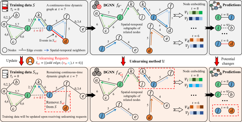
Figure 4: An overview of the complex interaction between $S_{re}$ and $S_{ul}$. (1) In the upper half, given a dynamic graph $S$ (maximum event time $T_{S}=8$) and a DGNN $f$, we use an algorithm $\mathcal{A}_{f}$ to obtain the optimal $f_{\theta^{*}}$, which can make accurate predictions on both training ($t\leq T_{S}$) and test ($t>T_{S}$) data. (2) Green/blue/brown arrows indicate the spatial and temporal neighbours of node $v_{i}$/$v_{j}$/$v_{d}$ in the last 2 historical time points. As shown in the middle column, DGNNs generally use the derived spatial-temporal subgraphs to obtain the node embedding. By combining the embedding of two nodes, $f$ can predict whether there is an edge between them at specific time points. (3) In the lower half, upon receiving the unlearning request $S_{ul}$, an unlearning method aims to approximate the parameter obtained from retraining $f$ with $S_{ul}$. (4) The dashed box on the left indicates the change in training data. The middle dashed box identifies the changed spatial-temporal subgraph of node $v_{j}$, potentially resulting in changed embedding at time $t=8$. The right dashed box highlights the desired prediction change from the perspective of unlearning.

Any data change needs in the training data $S$ could potentially raise unlearning requests. Besides the unlearning requests in Section 3, other unlearning needs also exist in real-world applications for various reasons. For example, users may expect to unlearn some specific features (e.g., forgetting the gender and age information for system fairness) or labels (e.g., out-of-date tags of interest) [5].

Interaction between $S_{ul}$ and $S_{re}$. In AI systems for general data (e.g., image or tabular data), $S_{ul}$ and $S_{re}$ are independent of each other, since the samples in the training dataset are independent and identically distributed (IID). However, for (static) graph data, $S_{ul}$ and $S_{re}$ can potentially interact with each other [7]. For example, given an unlearning node $v_{i}\in S_{ul}$, its connected neighbour nodes may belong to the remaining dataset $S_{re}$. Due to the message passing mechanism and stacking layer operation in most GNNs, existing studies have proposed to consider multi-hop neighbours when unlearning is performed for GNNs [10].

As shown in Figure 4, DGNNs are designed to learn both spatial and temporal information in dynamic graphs, making the interaction between $S_{ul}$ and $S_{re}$ in dynamic graphs more complex than that in static graphs. For example, in a dynamic graph neural network $f$ for CTDG data, the embedding of a node at time $t$ is obtained by taking into account its spatial and historical neighbour nodes. In the context of unlearning a DGNN $f_{\theta^{*}}$, i.e., obtaining the desired parameter $\theta^{*}_{ul}$ with an unlearning method $\mathcal{U}$, the complex interaction between $S_{ul}$ and $S_{re}$ includes:

• Changed predictions on invariant representations. Before and after removing $S_{ul}$ from $S$, an event $o_{i}$ in $S_{ul}$ may have observed the same series of events that remained in $S_{re}$ before its occurrence time, where spatial-temporal subgraphs are prone to generating almost invariant node embedding. However, the unlearning method $\mathcal{U}$ expects $f$ to make different predictions (e.g., $(v_{d},v_{j})$ at $t=6$).

• Invariant predictions on changed representations. Due to the removal of $S_{ul}$, the spatial-temporal neighbours of an event $o_{j}\in S_{re}$ are potentially different (e.g., $v_{j}$ at $t=8$), while the unlearning method $\mathcal{U}$ expects $f$ to make invariant predictions (e.g., there is an edge $(v_{i},v_{j})$ at $t=8$). Note that it is also not trivial to identify exactly the events in $S_{re}$ that are influenced by the unlearning request $S_{ul}$.

Appendix D Examples of Avoiding Overfitting Unlearning Data

As shown in Figure 5, in the remaining training data $S_{re}$, there is an edge event between $v_{a}$ and $v_{i}$ at time $t=5/7$ because they share a common neighbour node at the last time point (i.e., there are edges $(v_{a},v_{c})$ and $(v_{i},v_{c})$ at $t=4/6$). Although samples with the same pattern have been included in $S_{ul}$ (e.g., the edge $(v_{j},v_{d})$ at $t=6$ because they share the same neighbour $v_{f}$ in $t=5$), a well-retrained model $f$ can generalise well on $S_{ul}$ when a lot of samples with the same patterns have been kept in the remaining data $S_{re}$. Therefore, focussing on $100\%$ unlearning of $S_{ul}$ (e.g., there is no edge prediction in $S_{ul}$ with $100\%$ accuracy) potentially harms the performance of DGNNs on $S_{re}$.

The example in Figure 5 and the practical evaluation results on $S_{ul}$ by retraining (i.e., Tables 3 and 5) support us in using the results from the retraining method as the only gold standard to evaluate other unlearning methods. Our efforts to alleviate overfitting $S_{ul}$ also include setting $\beta=0.1$ in the loss function (11).

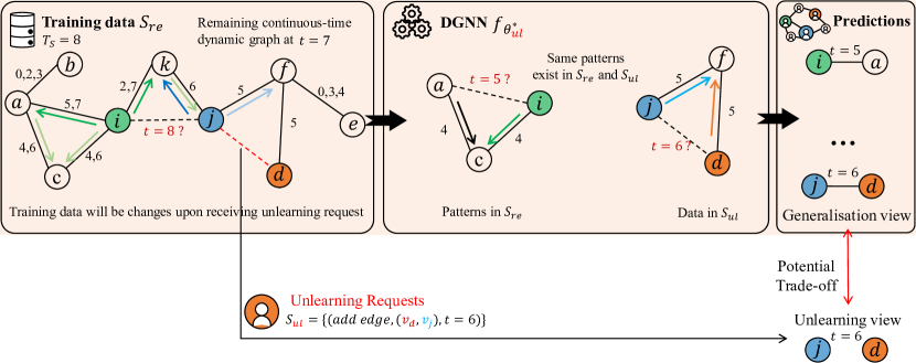
Figure 5: An illustration of the potential trade-off between model generalisation and unlearning requests on the training dataset. See Appendix D for more details.

Appendix E Datasets and Backbone DGNNs

Datasets. The six datasets in this paper are commonly used in the current study of dynamic graph neural networks [27, 30], and these datasets can be publicly accessed at the zenodo library. Table 4 presents the basic statistics of these datasets.

Table 4: Statistics of the datasets in this paper.

Datasets	Domains	#Nodes	#Links	Bipartite	Duration	Unique Steps	Time Granularity
Wikipedia	Social	9,227	157,474	True	1 month	152,757	Unix timestamps
UCI	Social	1,899	59,835	False	196 days	58,911	Unix timestamps
Reddit	Social	10,984	672,447	True	1 month	669,065	Unix timestamps
Enron	Social	184	125,235	False	3 years	22,632	Unix timestamps
MOOC	Interaction	7,144	411,749	True	17 months	345,600	Unix timestamps
LastFM	Interaction	1,980	$1,293,103$	True	1 month	$1,283,614$	Unix timestamps

DGNNs. In this paper, we focus on the following DGNN methods, which have different types of architecture, to evaluate the performance of unlearning methods.

• DyGFormer. Motivated by the fact that most existing methods overlook inter-node correlations within interactions, a method called DyGFormer [30] proposes a transformer-based architecture, which achieves the SOTA performance on dynamic graph tasks like link prediction and node classification.

• GraphMixer. In GraphMixer [34], a simple MLP-mixer architecture is used to achieve faster convergence and better generalisation performance, excluding complex modules such as recurrent neural networks and self-attention mechanisms, which are employed as de facto techniques to learn spatial-temporal information in dynamic graphs.

Appendix F Additional Evaluation Results

F.1 Original Model vs Unlearned Model Classification

As far as we know, there are no inference methods designed for dynamic graph neural networks, which can infer if an edge is in the training data of the model for link prediction. To evaluate the degree of unlearning, we compare the prediction similarity between the models obtained by our method and the retrained/original model, based on which we assign a class label to the prediction results derived from our method.

According to the motivation of machine unlearning [2], unlearning methods aim to remove the influence of the unlearning data and make the target model forget the knowledge learnt from these data, which can be used to serve users during the inference time of models. Therefore, we consider the predictions from the test data $Y_{te}^{(our)}$, $Y_{te}^{(ori)}$, $Y_{te}^{(retrain)}$ as inputs of Eq. (12) to evaluate the unlearning effectiveness from the perspective of ultimate unlearning goal (i.e., $f_{{\theta^{*}+\Delta\theta}}(S_{te})=f_{\theta^{*}_{ul}}(S_{te})$). Here, we compare the predictions with the test data, on which the unlearned model will be employed to serve users.

Classification Method. Assume that the predictions obtained from the original model, retrained model, and the model using our method are denoted as $Y^{(ori)}$, $Y^{(retrain)}$, and $Y^{(our)}$, respectively. If $Y^{(our)}$ is regarded as coming from the original model $f_{\theta^{*}}$, the assigned class label $\mathtt{C}$ for $Y^{(our)}$ will be $\mathtt{C}(Y^{(our)})=\mathtt{C}(Y^{(ori)})=\mathtt{C}_{\theta^{*}}$; otherwise, $\mathtt{C}(Y^{(our)})=\mathtt{C}(Y^{(retrain)})=\mathtt{C}_{\theta^{*}_{ul}}$. Specifically, (1) we obtain the prediction similarity by calculating the percentage of the same predictions, that is, $\mathtt{Acc}(Y^{(our)},Y^{(ori)})$ and $\mathtt{Acc}(Y^{(our)},Y^{(retrain)})$. (2) We treat $Y^{(ori)}$ and $Y^{(retrain)}$ as the class centre, and use the 1-nearest neighbor method to categorise $Y^{(our)}$ into the original or unlearned model class. Therefore, the label of $Y^{(our)}$ is obtained by

$$\mathtt{C}(Y^{(our)})=\begin{cases}\mathtt{C}_{\theta^{*}_{ul}},&if\ \mathtt{Acc}(Y^{(our)},Y^{(retrain)})>\mathtt{Acc}(Y^{(our)},Y^{(ori)})\\ \mathtt{C}_{\theta^{*}},&if\ \mathtt{Acc}(Y^{(our)},Y^{(retrain)})\leq\mathtt{Acc}(Y^{(our)},Y^{(ori)})\\ \end{cases}$$ (12)

Classification Results. Our approach successfully generates an unlearned model with an average likelihood of $81.33\%$, based on predictions from test data across all (dataset, DGNN) combinations, where each case is executed five times. These results further validate the effectiveness of our method in conducting an approximate unlearning of DGNNs.

F.2 Other Results

F.2.1 Evaluations on additional DGNN architecture

To further verify that our method is independent of the DGNN architecture, we evaluate the performance of our method on the CAWN model [35]. To obtain node embeddings, CAWN [35] samples random walks for each node and uses the anonymous identity to denote the nodes in these walks, which helps capture and extract multiple causal relationships in dynamic graphs. Table 5 shows the comparison between our method and baseline methods on the CAWN model.

F.2.2 Evaluations on future unlearning requests

Table 5: Comparison between our method and baseline methods on the CAWN model

[flushleft] Datasets Methods $\mathtt{Acc}(S_{re})/\Delta\mathtt{Acc}\uparrow$ $\mathtt{Acc}(S_{ul})/|\Delta\mathtt{Acc}|\downarrow$ $\mathtt{AUC}(S_{te})/\Delta\mathtt{AUC}\uparrow$ $\mathtt{t}_{ave}(s)$ Speed-up Wikipedia Re-training 0.9491 ± 0.0006 0.1159 ± 0.0048 0.9841 ± 0.0002 1903.3736 1 $\times$ Fine-tuning-ul 0.9485 ± 0.0015 0.1191 ± 0.0091 0.9820 ± 0.0014 526.8222 3.61$\times$ Fine-tuning 0.9485 ± 0.0015 0.1133 ± 0.0074 0.9814 ± 0.0021 568.0133 3.35$\times$ Ours 0.9486 ± 0.0007 0.1086 ± 0.0046 0.9829 ± 0.0001 263.2861 7.23$\times$ Reddit Re-training 0.9429 ± 0.0009 0.0411 ± 0.0029 0.9890 ± 0.0002 7449.4465 1$\times$ Fine-tuning-ul 0.6599 ± 0.0971 0.4201 ± 0.2954 0.6759 ± 0.1405 2500.3047 2.98$\times$ Fine-tuning 0.9041 ± 0.0034 0.4559 ± 0.0402 0.9640 ± 0.0013 3623.2015 2.06$\times$ Ours 0.9481 ± 0.0012 0.0303 ± 0.0022 0.9897 ± 0.0001 1329.4738 5.60$\times$ Enron Re-training 0.9094 ± 0.0018 0.1192 ± 0.0061 0.8758 ± 0.0094 1334.3856 1$\times$ Fine-tuning-ul 0.5399 ± 0.0744 0.6818 ± 0.3898 0.5970 ± 0.0591 537.0440 2.48$\times$ Fine-tuning 0.8600 ± 0.0190 0.2534 ± 0.0708 0.8403 ± 0.0221 612.8398 2.18$\times$ Ours 0.9162 ± 0.0007 0.1120 ± 0.0026 0.9024 ± 0.0007 291.0586 4.58$\times$

• $\mathtt{Acc}(S_{re})$ results represent the model performance on remaining training data, and the results (excluding the retraining method) with largest $\Delta\mathtt{Acc}$ is highlighted in bold. $\mathtt{Acc}(S_{ul})$ results indicates the model performance on unlearning data, and the results with smallest $|\Delta\mathtt{Acc}|$ are highlighted in bold. Underline points out the result where there is extremely overfitting on unlearning requests. $\mathtt{AUC}(S_{te})$ results show the model performance on test data, and the the results (excluding the retraining method) with largest $\Delta\mathtt{AUC}$ is highlighted in bold.

Table 6: Comparison between our method and retraining methods on the Wikipedia dataset when implementing future unlearning requests

[flushleft] $\mathtt{Acc}(S_{re})$ $\mathtt{Acc}(S_{ul})$ $\mathtt{AUC}(S_{te})$ $\mathtt{t}_{ave}$(s) Speed-up Retraining 0.9525 ± 0.0009 0.0514 ± 0.0035 0.9869 ± 0.0005 506.4784 1 $\times$ DyGFormer Ours 0.9569 ± 0.0065 0.0722 ± 0.0099 0.9853 ± 0.0004 16.2926 31.09 $\times$ Retraining 0.9077 ± 0.0056 0.0977 ± 0.0079 0.9610 ± 0.0031 500.6417 1 $\times$ GraphMixer Ours 0.9278 ± 0.0119 0.0803 ± 0.0296 0.9600 ± 0.0137 19.9474 25.10 $\times$ Retraining 0.9495 ± 0.0007 0.0749 ± 0.0013 0.9837 ± 0.0002 1594.1584 1 $\times$ CAWN Ours 0.9570 ± 0.0047 0.0803 ± 0.0199 0.9830 ± 0.0002 48.9181 32.59 $\times$

As shown in Table 6, we compared our method with the retraining method in the Wikipedia dataset when implementing future unlearning requests, which indicates the additional benefits of our method. Due to the training of our method in the previous unlearning process, the evaluation results suggest that it can potentially be used to directly infer the desired parameter update w.r.t. future unlearning requests. Table 6 shows that, in response to future unlearning requests, our approach can produce an unlearned model with a prediction accuracy comparable to the retraining method across the remaining, unlearning, and test data. Importantly, for such unlearning requests, our method can achieve an impressive speed increase, ranging from $25.10\times$ to $32.50\times$.

F.2.3 Evaluations on unlearning efficiency

Figure 6 demonstrates the efficiency advantage of our method. For most (dataset, DGNN) combination cases, our method obtained obvious efficiency advantages such as $6.36\times$ speeding up in the case (Reddit, GraphMixer). However, in the (LastFM, DyGFormer) case, the slight slowness can be attributed to the following reasons.

• The time cost increases when the amount of unlearning samples increases. Note that one typical advantage of our method is that it can deal with a batch of unlearning requests at once. After checking the code, we found that almost half of the training events (48%, unlearn 621445 events, while the total event number is 1293103) are used to compare the performance of different unlearning methods in this case. Compared with only limited unlearning samples (for example, one unlearning sample at a time [8]), the retraining method has fewer training dataset (i.e., the remaining data) when the amount of unlearning sample is larger.

• There is a potential trade-off between the unlearning samples and the remaining samples (as shown in Figure 5). Compared with the retraining method, which only focusses on improving model performance in 52% of the remaining data, other unlearning methods navigating the balance between remaining data and unlearning data generally have a slower rate of convergence, especially when the size difference between remaining and unlearning data is small.

Note that this harsh case (i.e., almost half of the training samples need to be unlearned) is not common in practical scenarios where only a limited ratio of training samples need to be unlearned. As shown in Figure 6, our method has an obvious efficiency advantage in most cases when unlearning a group of requests.

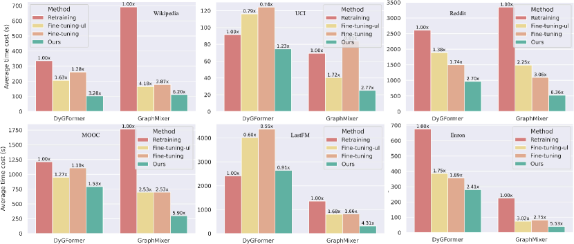
Figure 6: The time cost comparison between our Gradient Transformation method and baseline methods. The numerical values on the bars (e.g., $6.20\times$) indicate the degree of acceleration relative to the retraining approach.

References

- [1] Thanh Tam Nguyen, Thanh Trung Huynh, Phi Le Nguyen, Alan Wee-Chung Liew, Hongzhi Yin, and Quoc Viet Hung Nguyen. A survey of machine unlearning. CoRR, abs/2209.02299, 2022.
- [2] Heng Xu, Tianqing Zhu, Lefeng Zhang, Wanlei Zhou, and Philip S. Yu. Machine unlearning: A survey. ACM Comput. Surv., 56(1):9:1–9:36, 2024.
- [3] European Union. Right to be Forgotten, General Data Protection Regulation. https://gdpr-info.eu/issues/right-to-be-forgotten/, 2021.
- [4] Jinyin Chen, Haiyang Xiong, Haibin Zheng, Jian Zhang, and Yi Liu. Dyn-backdoor: Backdoor attack on dynamic link prediction. IEEE Trans. Netw. Sci. Eng., 11(1):525–542, 2024.
- [5] Alexander Warnecke, Lukas Pirch, Christian Wressnegger, and Konrad Rieck. Machine unlearning of features and labels. In NDSS. The Internet Society, 2023.
- [6] Bang Wu, He Zhang, Xiangwen Yang, Shuo Wang, Minhui Xue, Shirui Pan, and Xingliang Yuan. Graphguard: Detecting and counteracting training data misuse in graph neural networks. In NDSS, 2024.
- [7] Anwar Said, Tyler Derr, Mudassir Shabbir, Waseem Abbas, and Xenofon D. Koutsoukos. A survey of graph unlearning. CoRR, abs/2310.02164, 2023.
- [8] Min Chen, Zhikun Zhang, Tianhao Wang, Michael Backes, Mathias Humbert, and Yang Zhang. Graph unlearning. In CCS, pages 499–513. ACM, 2022.
- [9] Jiancan Wu, Yi Yang, Yuchun Qian, Yongduo Sui, Xiang Wang, and Xiangnan He. GIF: A general graph unlearning strategy via influence function. In WWW, pages 651–661. ACM, 2023.
- [10] Kun Wu, Jie Shen, Yue Ning, Ting Wang, and Wendy Hui Wang. Certified edge unlearning for graph neural networks. In KDD, pages 2606–2617. ACM, 2023.
- [11] Srijan Kumar, Xikun Zhang, and Jure Leskovec. Predicting dynamic embedding trajectory in temporal interaction networks. In KDD, pages 1269–1278. ACM, 2019.
- [12] Joakim Skarding, Bogdan Gabrys, and Katarzyna Musial. Foundations and modeling of dynamic networks using dynamic graph neural networks: A survey. IEEE Access, 9:79143–79168, 2021.
- [13] Zonghan Wu, Shirui Pan, Guodong Long, Jing Jiang, and Chengqi Zhang. Graph wavenet for deep spatial-temporal graph modeling. In IJCAI, pages 1907–1913. ijcai.org, 2019.
- [14] Chong Chen, Fei Sun, Min Zhang, and Bolin Ding. Recommendation unlearning. In WWW, pages 2768–2777. ACM, 2022.
- [15] Zizhang Chen, Peizhao Li, Hongfu Liu, and Pengyu Hong. Characterizing the influence of graph elements. In ICLR. OpenReview.net, 2023.
- [16] Yang Zhang, Zhiyu Hu, Yimeng Bai, Fuli Feng, Jiancan Wu, Qifan Wang, and Xiangnan He. Recommendation unlearning via influence function. CoRR, abs/2307.02147, 2023.
- [17] Weilin Cong and Mehrdad Mahdavi. Efficiently forgetting what you have learned in graph representation learning via projection. In AISTATS, volume 206 of Proceedings of Machine Learning Research, pages 6674–6703. PMLR, 2023.
- [18] Jiali Cheng, George Dasoulas, Huan He, Chirag Agarwal, and Marinka Zitnik. Gnndelete: A general strategy for unlearning in graph neural networks. In ICLR. OpenReview.net, 2023.
- [19] Cheng-Long Wang, Mengdi Huai, and Di Wang. Inductive graph unlearning. In USENIX Security Symposium, pages 3205–3222. USENIX Association, 2023.
- [20] Eli Chien, Chao Pan, and Olgica Milenkovic. Certified graph unlearning. In NeurIPS 2022 Workshop: New Frontiers in Graph Learning, 2022.
- [21] M. Seyed Kazemi. Dynamic graph neural networks. In Lingfei Wu, Peng Cui, Jian Pei, and Liang Zhao, editors, Graph Neural Networks: Foundations, Frontiers, and Applications, pages 323–349. Springer Singapore, Singapore, 2022.
- [22] Seongjun Yun, Minbyul Jeong, Raehyun Kim, Jaewoo Kang, and Hyunwoo J. Kim. Graph transformer networks. In NeurIPS, pages 11960–11970, 2019.
- [23] Ao Zhou, Jianlei Yang, Yeqi Gao, Tong Qiao, Yingjie Qi, Xiaoyi Wang, Yunli Chen, Pengcheng Dai, Weisheng Zhao, and Chunming Hu. Brief industry paper: optimizing memory efficiency of graph neural networks on edge computing platforms. In RTAS, pages 445–448. IEEE, 2021.
- [24] Nicola De Cao, Wilker Aziz, and Ivan Titov. Editing factual knowledge in language models. In EMNLP (1), pages 6491–6506. Association for Computational Linguistics, 2021.
- [25] Seyed Mehran Kazemi, Rishab Goel, Kshitij Jain, Ivan Kobyzev, Akshay Sethi, Peter Forsyth, and Pascal Poupart. Representation learning for dynamic graphs: A survey. J. Mach. Learn. Res., 21:70:1–70:73, 2020.
- [26] Thomas N. Kipf and Max Welling. Semi-supervised classification with graph convolutional networks. In ICLR (Poster). OpenReview.net, 2017.
- [27] Farimah Poursafaei, Shenyang Huang, Kellin Pelrine, and Reihaneh Rabbany. Towards better evaluation for dynamic link prediction. In NeurIPS, 2022.
- [28] Shenyang Huang, Farimah Poursafaei, Jacob Danovitch, Matthias Fey, Weihua Hu, Emanuele Rossi, Jure Leskovec, Michael M. Bronstein, Guillaume Rabusseau, and Reihaneh Rabbany. Temporal graph benchmark for machine learning on temporal graphs. CoRR, abs/2307.01026, 2023.
- [29] Edward Newell, David Jurgens, Haji Mohammad Saleem, Hardik Vala, Jad Sassine, Caitrin Armstrong, and Derek Ruths. User migration in online social networks: A case study on reddit during a period of community unrest. In ICWSM, pages 279–288. AAAI Press, 2016.
- [30] Le Yu, Leilei Sun, Bowen Du, and Weifeng Lv. Towards better dynamic graph learning: New architecture and unified library. In NeurIPS, 2023.
- [31] Werner Zellinger, Thomas Grubinger, Edwin Lughofer, Thomas Natschläger, and Susanne Saminger-Platz. Central moment discrepancy (CMD) for domain-invariant representation learning. In ICLR (Poster). OpenReview.net, 2017.
- [32] Pietro Panzarasa, Tore Opsahl, and Kathleen M. Carley. Patterns and dynamics of users’ behavior and interaction: Network analysis of an online community. J. Assoc. Inf. Sci. Technol., 60(5):911–932, 2009.
- [33] Jitesh Shetty and Jafar Adibi. The enron email dataset database schema and brief statistical report. Information sciences institute technical report, University of Southern California, 4(1):120–128, 2004.
- [34] Weilin Cong, Si Zhang, Jian Kang, Baichuan Yuan, Hao Wu, Xin Zhou, Hanghang Tong, and Mehrdad Mahdavi. Do we really need complicated model architectures for temporal networks? In ICLR. OpenReview.net, 2023.
- [35] Yanbang Wang, Yen-Yu Chang, Yunyu Liu, Jure Leskovec, and Pan Li. Inductive representation learning in temporal networks via causal anonymous walks. In ICLR. OpenReview.net, 2021.
- [36] Hao Peng, Bowen Du, Mingsheng Liu, Mingzhe Liu, Shumei Ji, Senzhang Wang, Xu Zhang, and Lifang He. Dynamic graph convolutional network for long-term traffic flow prediction with reinforcement learning. Inf. Sci., 578:401–416, 2021.
- [37] Guotong Xue, Ming Zhong, Jianxin Li, Jia Chen, Chengshuai Zhai, and Ruochen Kong. Dynamic network embedding survey. Neurocomputing, 472:212–223, 2022.
- [38] Joshua Fan, Junwen Bai, Zhiyun Li, Ariel Ortiz-Bobea, and Carla P. Gomes. A GNN-RNN approach for harnessing geospatial and temporal information: Application to crop yield prediction. In AAAI, pages 11873–11881. AAAI Press, 2022.
- [39] Da Xu, Chuanwei Ruan, Evren Körpeoglu, Sushant Kumar, and Kannan Achan. Inductive representation learning on temporal graphs. In ICLR. OpenReview.net, 2020.
- [40] Rakshit Trivedi, Mehrdad Farajtabar, Prasenjeet Biswal, and Hongyuan Zha. Dyrep: Learning representations over dynamic graphs. In ICLR (Poster). OpenReview.net, 2019.
- [41] Emanuele Rossi, Ben Chamberlain, Fabrizio Frasca, Davide Eynard, Federico Monti, and Michael M. Bronstein. Temporal graph networks for deep learning on dynamic graphs. CoRR, abs/2006.10637, 2020.
- [42] Chao Pan, Eli Chien, and Olgica Milenkovic. Unlearning graph classifiers with limited data resources. In WWW, pages 716–726. ACM, 2023.