Exact Gauss-Newton Optimization
for Training Deep Neural Networks
| Mikalai Korbit† and Adeyemi D. Adeoye† and Alberto Bemporad† and Mario Zanon† |
| DYSCO (Dynamical Systems, Control, and Optimization)† |
| IMT School for Advanced Studies Lucca, Italy |
Abstract
We present EGN, a stochastic second-order optimization algorithm that combines the generalized Gauss-Newton (GN) Hessian approximation with low-rank linear algebra to compute the descent direction. Leveraging the Duncan-Guttman matrix identity, the parameter update is obtained by factorizing a matrix which has the size of the mini-batch. This is particularly advantageous for large-scale machine learning problems where the dimension of the neural network parameter vector is several orders of magnitude larger than the batch size. Additionally, we show how improvements such as line search, adaptive regularization, and momentum can be seamlessly added to EGN to further accelerate the algorithm. Moreover, under mild assumptions, we prove that our algorithm converges to an -stationary point at a linear rate. Finally, our numerical experiments demonstrate that EGN consistently exceeds, or at most matches the generalization performance of well-tuned SGD, Adam, and SGN optimizers across various supervised and reinforcement learning tasks.
1 Introduction
Optimization plays a pivotal role in Machine Learning (ML), with gradient-based methods being at the forefront. Stochastic Gradient Descent (SGD) [61], a first-order stochastic optimization algorithm, and its accelerated versions such as momentum-based approaches [51, 67, 44, 16], adaptive learning rates [22, 30, 81], and a combination of the two [36, 21, 80], have been instrumental in numerous ML applications. For example, in Computer Vision (CV) ResNets [29] are trained with SGD, AdaGrad [22] is used for training recommendation systems [50], language models GPT-3 [12] and LLaMA [69] are optimized with Adam [36] and AdamW [43], respectively. Despite their cheap and relatively easy-to-implement updates, first order-methods (FOMs) suffer from several shortcomings. FOMs are sensitive to hyper-parameter selection, and the optimal hyper-parameter set typically does not transfer well across different problems which leads to a costly procedure of hyper-parameter tuning. Also, FOMs are slow to converge in the flat regions of the loss landscape, where the Hessian is ill-conditioned [62].
Second-order methods (SOMs) incorporate the (approximate) curvature information into the update in order to effectively precondition the gradient vector. In contrast to first-order algorithms, SOMs are shown to be robust to the selection of hyper-parameters [77] and to potentially offer faster convergence [2, 6]. So far, the adoption of second-order methods for ML problems has been limited due to the complexity in calculating and storing the Hessian and the computational load of solving the linear system , where is the (approximate) Hessian matrix, is the gradient of the loss function, and is the descent direction. Addressing these computational challenges, most approaches use a combination of Hessian approximation and an efficient algorithmic technique for solving the linear system. Common approximations to the Hessian include diagonal scaling [78, 42], the empirical Fisher matrix [60], the quasi-Newton approach [65, 14, 5], and the Gauss-Newton (GN) approximation [24, 70, 13].
In this work, we follow the Gauss-Newton approach to Hessian approximation. Our innovation is in the use of an efficient exact linear algebra identity—the Duncan-Guttman (DG) formula [23, 26]—to speed up the inversion of the Hessian matrix. Compared to Hessian-free optimization (HFO) [46, 47, 37] and Inexact Gauss-Newton (iGN) [70], Exact Gauss-Newton (EGN) solves the system exactly with the same algorithmic complexity burden. The closest approach to EGN, to the best of our knowledge, is the application of the Sherman–Morrison-Woodbury (SMW) formula [60]. As we outline below, by using a different matrix identity we are able to solve for the descent direction in fewer matrix operations than SWM, thus reducing the algorithmic complexity.
Our contributions are as follows.
-
•
We propose the EGN algorithm, which relies on a regularized Gauss-Newton Hessian matrix and exploits the Duncan-Guttman identity to efficiently solve the linear system.
-
•
We provide a theoretical analysis of the EGN algorithm and establish an algorithmic upper bound on the complexity of EGN in finding an -stationary point.
-
•
We evaluate the performance of EGN on several supervised learning and reinforcement learning tasks using various neural network architectures.
2 Preliminaries
2.1 Notation
We use boldface letters to denote vectors and matrices. The identity matrix is denoted by , and we omit the subscript when the size is clear from the context. The subscript represents the iteration within the optimization loop, and may be omitted to avoid overloading the notation. We define the standard inner product between two vectors as . The standard Euclidean norm is denoted by , and the expected value of a random variable is denoted by .
2.2 Problem Formulation
We adopt the Empirical Risk Minimization (ERM) framework [49] and consider the problem of finding the weights of a parametric function , e.g., a neural network, such that it minimizes the empirical risk over a dataset consisting of pairs where is a vector of features and , is a target vector. We want to solve the following optimization problem:
| (2.1) |
where is a random variable with distribution . The objective function is expressed as a finite-sum of functions over the realization of , and
| (2.2) |
is the empirical risk with – a loss function, involving a single pair only.
We assume all these functions to be twice differentiable with respect to . Note that, while this assumption could be partially relaxed, we stick to it for the sake of simplicity.
2.3 Gradient-based Optimization
Problem (2.1) is typically solved by variations of the Stochastic Gradient Descent (SGD) method by sampling mini-batches from rather than processing the entire dataset in each iteration. We denote the loss on a mini-batch as
| (2.3) |
where is the batch size. The iterations take the form
| (2.4) |
where is a learning rate and is a descent direction obtained from the gradient. In general, we have where is a preconditioning matrix that scales, rotates, and shears the gradient of the mini-batch loss . Notice that by setting , and we recover the incremental SGD update [61]. In practice, the preferred training algorithm is often an accelerated version of mini-batch SGD.
Minimizing the quadratic approximation of the batch loss leads to the following linear system
| (2.5) |
where is the Hessian matrix of the mini-batch loss. Finding the direction by solving the system (2.5) using or its approximation defines the broad spectrum of second-order methods. Setting results in Newton’s method. This method suffers from several drawbacks: (a) one needs to compute second-order derivatives with respect to ; (b) has to be positive-definite to ensure descent; (c) the linear system (2.5) must be solved, which in general scales cubically with the dimension of ; and (d) since is a noisy estimate of the true Hessian of the empirical risk , can result in suboptimal conditioning. These issues and the fact that is of rather large dimension have made the direct application of Newton’s method practically irrelevant in ML applications. Indeed, for problems like Large Language Model (LLM) pre-training [71, 12, 69] or CV tasks [29], can be extremely high-dimensional, e.g., parameters for Grok-1 [76] model, to parameters for LLaMA-family models [69] and to parameters for ResNets [29], which explains why accelerated first-order methods are usually preferred.
In order to make SOMs scalable for ML applications one could instead approximate the inverse Hessian, i.e., . Examples of such preconditioning include diagonal scaling (e.g., with Hutchinson method [78, 42]) with the idea of extracting the (approximate) diagonal elements of while neglecting the off-diagonal terms; the quasi-Newton approach [14, 5] that approximates the Hessian using the information from past and current gradients; and the Gauss-Newton method [24, 60] that leverages the Jacobian of the residuals, neglecting second-order cross-derivatives, particularly suitable for loss functions structured as (2.2). In this paper, we use the Gauss-Newton Hessian approximation which is shown to provide a good approximation of the true Hessian for ML applications [62, 56].
2.4 Generalized Gauss-Newton Hessian Approximation
We consider the Generalized Gauss-Newton (GGN) Hessian approximation scheme [64, 8, 56] which is suited for both regression and multi-class classification tasks.
The GGN Hessian approximation is constructed using only first-order sensitivities (see derivation in Appendix B) to obtain
| (2.6) |
where we vertically stack individual Jacobians for each sample in the batch to form and construct a block diagonal matrix , where . As pointed out in [63], approximation (2.6) is justified since the true Hessian is dominated by the term . Using the inverse of the GGN Hessian as a preconditioner yields the following direction
| (2.7) |
which, by defining , corresponds to the solution of the quadratic program
| (2.8) |
The Gauss-Newton step (2.7) solves issues (a) and, partially, (b), since no second-order derivatives need to be computed and the Hessian approximation is positive semi-definite by construction provided that the loss function is convex. A positive-definite Hessian approximation can easily be obtained from , e.g., by adding to it a small constant times the identity matrix. This approach is called Levenberg-Marquardt (LM) [53] and is often used in practice, such that
| (2.9) |
with . The regularizer serves a dual purpose: it ensures that the approximate Hessian matrix is invertible and also it helps to avoid over-fitting [49].
The Gauss-Newton update, however, still potentially suffers from issue (c), i.e., the need to solve a linear system, which can be of cubic complexity, and (d) the noise in the Hessian estimate. Since issue (c) is a centerpiece of our method, and issue (d) is an inherent part of stochastic sampling we defer the discussion on both of them to Section 3.
We conclude by examining the GGN update in two common machine learning tasks—regression and multi-class classification—and how it is derived in each case.
Regression
Regression is a predictive modeling task where the objective is to predict a scalar numeric target. For regression tasks we define the loss function as the mean squared error (MSE)
| (2.10) |
We can show (see Appendix B.2) that the gradient and the GN Hessian for the MSE loss read
| (2.11) |
where is a matrix of stacked Jacobians, and is a vector of residuals defined as .
Multi-class Classification
The task of multi-class classification is to predict a correct class from classes given a vector of features . For such problems the output of the neural network is a -dimensional vector of prediction scores (logits) and the target vector is a one-hot encoded vector , where denotes column of the identity matrix and is the index of the correct class. We define the loss function as a softmax cross-entropy loss (CE)
| (2.12) |
where , and are -th elements of vectors and respectively.
As shown in Appendix B.3, the gradient and the GN Hessian for the CE loss are
| (2.13) |
where is a matrix of stacked Jacobians, is a vector of (pseudo-)residuals defined as , and is a block diagonal matrix of stacked matrices that each have across the diagonal and off-diagonal.
3 Algorithm
We are now ready to present the EGN algorithm. First, we will discuss how one can efficiently solve the linear system. Then, we will discuss further enhancements to the basic algorithm.
Next, we address issue (c), i.e., the problem of finding the solution of the symmetric linear system . Substituting the exact Hessian with the regularized Gauss-Newton Hessian yields
| (3.1) |
where for the MSE loss and . Solving (3.1) for requires one to factorize matrix , carrying a complexity of . We notice, however, that in practice one often has , i.e., the parameter vector is of very high dimension, e.g., . In that case, the GN Hessian matrix (2.6) is low-rank by construction. That allows us to transfer the computationally expensive inversion operation from the high-dimensional space (which is the original dimension of the Hessian) to the low-dimensional space.
Theorem 3.1
Assuming and are full-rank matrices, the following identity holds
| (3.2) |
By observing that Equation (3.1) defining the direction has the form of the left-hand side of the identity (3.2) we state the following (see proof in Appendix B.4).
Lemma 3.2
The key property of Algorithm 1 is that the system (2.5) is solved exactly in contrast to approximate (or inexact) solutions that underpin algorithms such as HFO [46, 37], Newton-SGI [6], LiSSA [2], SGN [24] and iGN [70]. The benefits of having the exact solution are analyzed in [6] with exact Newton methods enjoying faster convergence rates than inexact ones. Our experiments (Section 5) also demonstrate that the exact Gauss-Newton solver (EGN) consistently outperforms the inexact version (SGN) across the majority of the problems. The complexity of Algorithm 1 is dominated by the matrix multiplication that costs as well as solving the linear system of size with complexity . Assuming , the overall complexity of Algorithm 1 is .
An alternative approach to solve Equation (3.1) exactly is the SWM formula employed in [60, 13, 31, 4]. Solving (3.1) with the SWM formula yields . As with EGN, the dominating term is . However, even with efficient ordering of operations, there are at least two matrix multiplications while EGN requires just one. Another important consideration is the non-regularized case, i.e., when . Assuming is invertible, EGN produces a valid solution while SWM is not defined in that case. That makes Algorithm 1 a preferred choice for finding the direction (B.6) exactly.
For completeness, we note here that another option to solve (3.1) exactly is through a QR factorization of (see Appendix C). The complexity of such an approach is also , dominated by the economy size QR decomposition of . However, performing a QR decomposition is significantly more expensive than performing matrix-matrix multiplications and, in practice, EGN is preferred.
The CG method is an essential part of, e.g., HFO [46, 37], SGN [24], Newton-CG [6], LM [59], and Distributed Newton’s method with optimal shrinkage [82]. The complexity of CG approximately solving Equation (3.1) is where is the number of CG iterations [53]. A typical number of CG iterations ranges from in [37] to in [15]. Note that, unless the number of classes is high (which is one of the limitations of EGN addressed in Section 5.3), we have , such that EGN solves the system both exactly and faster than CG.
Besides estimating the Hessian-adjusted direction, most state-of-the-art SOMs employ strategies to reduce variance of gradient and Hessian estimates, safeguard against exploding gradients, and dynamically adjust hyper-parameters to training steps. In Appendix C we discuss several enhancements to EGN, including momentum acceleration [36, 37, 78] to mitigate issue (d), i.e., the noise in Hessian estimates; line search [17, 72, 59] to ensure steps are sufficiently short to decrease the loss; and adaptive regularization [37, 59, 60] to obtain faster convergence and simplify hyper-parameter tuning. The pseudocode for EGN is outlined in Algorithm 5 in Appendix C.
4 Convergence Analysis
In this section, we analyze the convergence of EGN (Algorithm 1) in the general non-convex setting. In EGN, we consider the sequence of iterates where each is computed via (2.4) with . We aim to minimize the function using, for each realization , the Hessian estimator and the gradient estimator . Then, at each iteration , the mini-batch estimates and of the gradient and Hessian are
| (4.1) |
In our analysis, we make use of the following assumptions.
Assumption 4.1
The function is lower-bounded on its domain, i.e., . In addition, is twice differentiable with Lipschitz continuous first-order derivatives, i.e., such that
| (4.2) |
Assumption 4.2
At any iteration , is an unbiased estimator of , i.e.,
| (4.3) |
Moreover, we have
| (4.4) |
where is a variance parameter.
Assumption 4.3
At any iteration , with . Moreover, satisfying such that for all .
Assumption 4.4
At any iteration , and for any random matrix satisfying with , , where .
In Lemma 4.1, we prove a descent lemma for EGN under the given conditions (see Appendix B.5 for the proof).
Lemma 4.1
Assumption 4.4 is necessary to prove the result in Lemma 4.1 due to the correlation between and . If these quantities were not correlated, then one could exploit Assumptions 4.2–4.3: by taking the expected value and using (4.3), one could then bound to obtain the desired bound with . Clearly, that would yield different constants in our next results, but their nature would remain unaltered. Note that this observation could suggest alternative versions of EGN, in which the correlation is removed by construction at the expense of an increased computational burden. A thorough investigation of such schemes is beyond the scope of this paper.
We next show the iteration complexity estimate of EGN to reach an -stationary point. We provide the proof in Appendix B.6.
Theorem 4.2
Let the assumptions in Lemma 4.1 hold, and assume is fixed for all . Let be a positive number such that holds for all . Then, if the mini-batch size is such that , the sequence , with , satisfies
| (4.6) |
Corollary 4.3
Suppose that the assumptions in Theorem 4.2 hold. Then, for any , the sequence satisfies after at most iterations, provided that .
5 Experiments
We conduct a series of experiments to measure the performance of EGN on several supervised learning and reinforcement learning tasks. We select three baseline solvers: SGD [61], Adam [36], and SGN [24]. SGD acts as a most basic baseline with the computationally cheapest update; Adam is a widely used accelerated FOM for training DNNs; SGN is an inexact Gauss-Newton solver against which we evaluate the practical advantages of solving the system (2.5) exactly. Since first-order methods typically require less computations per iterate, in order to obtain a fair comparison we monitor the wall time instead of the number of iterations. The learning rates are selected as the best performing after a grid search in the logspace . Additionally, for SGN we search for the optimal “number of CG iterations” within the set . For EGN we introduce two extra hyper-parameters: “line search” and “momentum” . The best performing sets of hyper-parameters as well as detailed description of the datasets are available in Appendix D. The size of the mini-batch for all problems is . All the experiments are conducted on the Tesla T4 GPU in the Google Colab environment with float32 precision.
5.1 Supervised Learning
For the regression task, we select three datasets: California Housing [55], Superconductivity [27], and Diamonds [74] with , , and training samples, respectively. For classification, we use the IMDB Reviews dataset [45] containing instances of movie reviews. Across all problems, the model is a Feedforward Neural Network (FFNN) with three dense layers of , and units followed by the ReLU activation function with a total of parameters (). The loss function during the training is a least-squares loss (2.10) for regression and softmax cross-entropy loss (2.12) for classification. The datasets are split into training and test sets in the proportion of percent. Numerical features are scaled and categorical features are one-hot encoded. To measure the performance, we plot the evolution of the evaluation metric on unseen data (test set) with respect to wall time (in seconds). The evaluation metric is Root Mean Squared Error (RMSE) for regression and accuracy for classification.
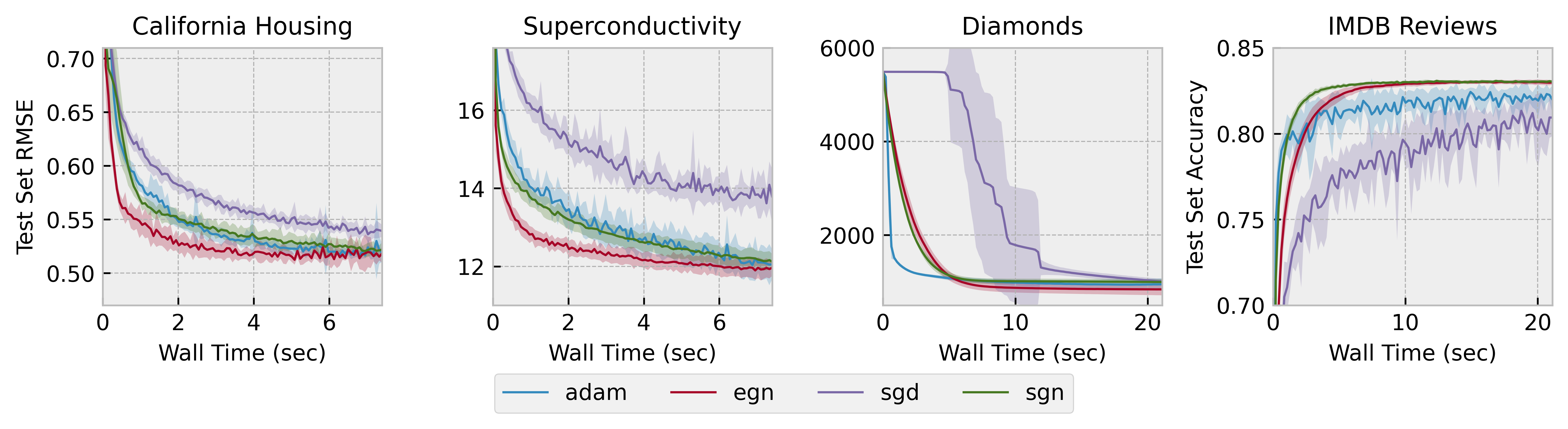
| Optimizer | California Housing | Superconduct | Diamonds | IMDB Reviews |
|---|---|---|---|---|
| SGD | 0.539 0.006 | 13.788 0.698 | 1008.936 54.940 | 0.809 0.011 |
| Adam | 0.519 0.009 | 12.052 0.381 | 947.258 130.079 | 0.820 0.008 |
| EGN | 0.518 0.009 | 11.961 0.207 | 840.500 126.444 | 0.830 0.001 |
| SGN | 0.522 0.007 | 12.121 0.196 | 998.688 61.489 | 0.830 0.001 |
The results are presented in Figure 1 and Table 1. On all but the IMDB Reviews dataset EGN has achieved both faster convergence and lower test set error than any other optimization algorithm. On IMDB Reviews SGN is faster than EGN, however, the two solvers achieve the same accuracy after reaching convergence.
5.2 Reinforcement Learning
We demonstrate the application of EGN to reinforcement learning in two scenarios: continuous action spaces with Linear-Quadratic Regulator (LQR) and discrete action spaces using Deep Q-Network (DQN) [48].
Learning LQR Controllers
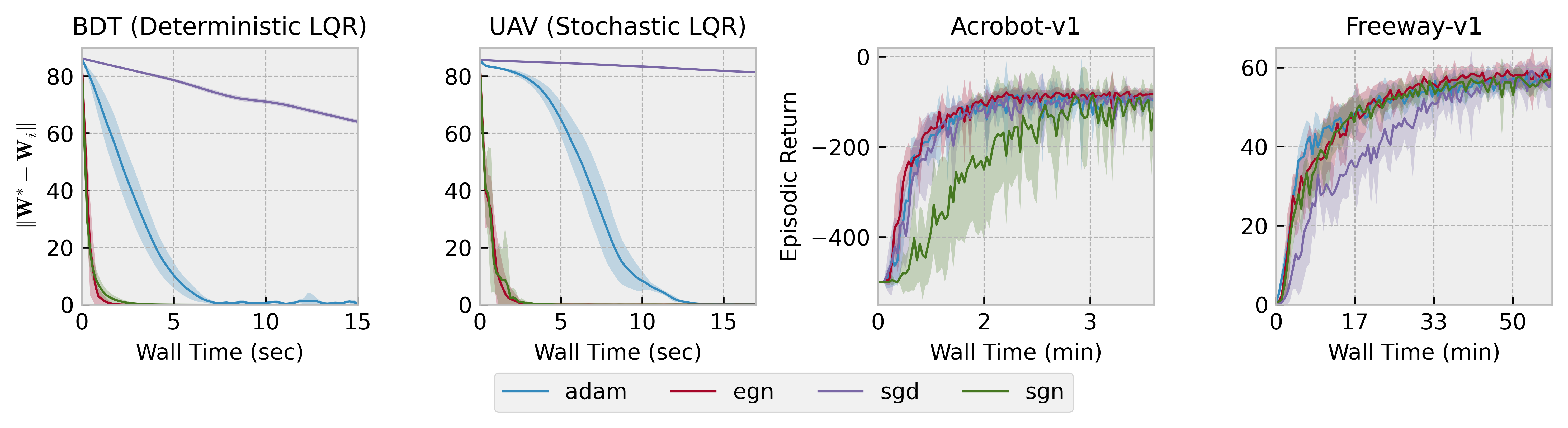
Given a discrete time-invariant linear system with continuous states and actions, and a quadratic reward function our task is to learn the optimal value function and the optimal policy such that we maximize the cumulative return. Such problems can be solved in a data-driven fashion with the policy iteration procedure [10] (outlined in Appendix D.2). It is well known that the optimal value function is quadratic and the optimal policy function is linear [28]. Consequently, we define as a quadratic function of states and actions. We track the norm of the difference between the optimal LQR controller calculated analytically knowing the system matrices and the learned weights of the model.
We select two linear systems from the Compleib set of benchmarks [39]. The first system is a deterministic model of a binary distillation tower (BDT) [18], and the second one represents the linearized vertical plane dynamics of an aircraft (UAV) with noise [34]. The results are displayed in the two leftmost charts of Figure 2 and Table 2. Both EGN and SGN outperform first-order methods by a considerable margin, with EGN enjoying slightly faster convergence in both cases, while SGN achieves a marginally lower error on the stochastic LQR upon reaching convergence.
Reinforcement Learning with DQN
Adopting the problem formulation of [48], we aim to learn the weights of a neural network that represents a -value function that maps states and actions into scores (-values) for a discrete set of actions. Once training is complete, the optimal policy is formed by calculating the -value of each action and choosing the highest-scoring action.
We build upon CleanRL [33] framework for running RL experiments, selecting two environments: Acrobot-v1 and Freeway-v1. Acrobot-v1 is an OpenAI gym [11] environment with a -dimensional state vector and a set of discrete actions where the goal is to swing the free end of the connected joints above a given height in as few steps as possible. Freeway-v1 is a MinAtar [79] environment that emulates the original Freeway Atari game. The state is represented by a image and there are discrete actions available. For Acrobot-v1 the network is a FFNN with three dense layers of , and units followed by the ReLU activation function with a total of parameters. For Freeway-v1 we design a compact CNN, comprising of a convolutional layer with sixteen filters and ReLU activation, followed by flattening, a -unit dense layer with ReLU, and a final dense layer outputting -values for all actions ().
| Optimizer | BDT | UAV | Acrobot-v1 | Freeway-v1 |
|---|---|---|---|---|
| SGD | ||||
| Adam | ||||
| EGN | 0.000 0.000 | -81.796 11.778 | 58.916 1.946 | |
| SGN | 0.000 0.000 | 0.033 0.019 |
The cumulative returns from each completed episode are recorded and displayed in the rightmost charts of Figure 2. The results for both Acrobot-v1 and Freeway-v1 show no distinct advantage among the solvers, as they all reach similar episodic returns. We notice, however, that EGN slightly outperforms other optimizers by achieving a higher return level at convergence (see Table 2).
5.3 Limitations
While delivering promising results, EGN also has some limitations, as we discuss below.
Explicit gradients
Unlike first-order methods that rely on the average gradient of the batch loss, Gauss-Newton methods require the full Jacobian matrix, which contains the gradients of each sample. As a result, backpropagation for EGN is more time-consuming than for FOMs. Moreover, this can lead to increased GPU memory usage, especially with high-dimensional parameter vectors.
Large batch sizes
In our experiments we observed that the cost of computing the derivatives and the subsequent cost of computing the step are approximately the same. However, for large batch sizes () and parameter dimensions (), we observed that the computational times increased significantly. We suspect this to be related to hardware limitations, and future research will aim to investigate this aspect in further detail.
Large number of classes for multi-class classification
By incorporating the softmax function into the loss equation (2.12) we introduce coupling between the individual outputs of in the denominator , which makes the Jacobian a dense matrix. Speeding up the calculation of remains an open research question and constitutes a major obstacle in using Gauss-Newton methods for tasks involving a large number of classes, e.g., LLM pre-training. One possible solution could consist in moving the softmax function directly into the model as the last layer of the network and then only computing the Jacobian wrt the correct class, resulting in . This approach, however, yields a Hessian approximation that becomes singular close to the solution, which results in numerical instabilities that hinder convergence [25]. Another possibility suggested in [54] consists in replacing the softmax cross-entropy loss with the multi-class hinge loss. Although the computation becomes faster for the hinge loss, empirical evidence shows that the test set accuracy upon training completion is higher for the CE loss. Finally, a promising approach is the Gauss-Newton-Bartlett (GNB) estimator proposed by [42], which replaces the exact LM Hessian with an approximation obtained by sampling the subset of predicted labels.
6 Conclusions and Future Work
We presented the EGN algorithm, a stochastic second-order method that efficiently estimates the descent direction by using a low-rank Gauss-Newton Hessian approximation and leveraging the Duncan-Guttman matrix identity. We demonstrated that EGN solves the system exactly with less computational burden than other exact Gauss-Newton methods, as well as inexact methods that rely on conjugate gradient iterates. We also proved that under mild assumptions our algorithm converges to an -stationary point at a linear rate. Our empirical results show that EGN consistently matches or exceeds the generalization performance of well-tuned SGD, Adam, and SGN optimizers across various supervised and reinforcement learning tasks.
Future work will focus on addressing the shortcomings of EGN in classification problems with a large number of classes. A promising direction is to approximate the Gauss-Newton Hessian matrix to avoid computing the full Jacobian of the network, e.g., using techniques such as the Gauss-Newton-Bartlett estimator [42]. Another direction is to study the performance of EGN on larger datasets and more complex models.
References
- [1] Adeyemi D Adeoye and Alberto Bemporad. SCORE: approximating curvature information under self-concordant regularization. Computational Optimization and Applications, 86(2):599–626, 2023.
- [2] Naman Agarwal, Brian Bullins, and Elad Hazan. Second-order stochastic optimization for machine learning in linear time. The Journal of Machine Learning Research, 18(1):4148–4187, 2017.
- [3] Shun-Ichi Amari. Natural gradient works efficiently in learning. Neural computation, 10(2):251–276, 1998.
- [4] Michael Arbel, Romain Menegaux, and Pierre Wolinski. Rethinking Gauss-Newton for learning over-parameterized models. Advances in Neural Information Processing Systems, 36, 2024.
- [5] Albert S Berahas, Jorge Nocedal, and Martin Takác. A multi-batch L-BFGS method for machine learning. Advances in Neural Information Processing Systems, 29, 2016.
- [6] Raghu Bollapragada, Richard H Byrd, and Jorge Nocedal. Exact and inexact subsampled Newton methods for optimization. IMA Journal of Numerical Analysis, 39(2):545–578, 2019.
- [7] Aleksandar Botev, Hippolyt Ritter, and David Barber. Practical Gauss-Newton optimisation for deep learning. In International Conference on Machine Learning, pages 557–565. PMLR, 2017.
- [8] Léon Bottou, Frank E Curtis, and Jorge Nocedal. Optimization methods for large-scale machine learning. SIAM review, 60(2):223–311, 2018.
- [9] Steven J Bradtke and Andrew G Barto. Linear least-squares algorithms for temporal difference learning. Machine learning, 22(1):33–57, 1996.
- [10] Steven J Bradtke, B Erik Ydstie, and Andrew G Barto. Adaptive linear quadratic control using policy iteration. In Proceedings of 1994 American Control Conference-ACC’94, volume 3, pages 3475–3479. IEEE, 1994.
- [11] Greg Brockman, Vicki Cheung, Ludwig Pettersson, Jonas Schneider, John Schulman, Jie Tang, and Wojciech Zaremba. OpenAI Gym, 2016.
- [12] Tom B. Brown, Benjamin Mann, Nick Ryder, Melanie Subbiah, Jared Kaplan, Prafulla Dhariwal, Arvind Neelakantan, Pranav Shyam, Girish Sastry, Amanda Askell, Sandhini Agarwal, Ariel Herbert-Voss, Gretchen Krueger, Tom Henighan, Rewon Child, Aditya Ramesh, Daniel M. Ziegler, Jeffrey Wu, Clemens Winter, Christopher Hesse, Mark Chen, Eric Sigler, Mateusz Litwin, Scott Gray, Benjamin Chess, Jack Clark, Christopher Berner, Sam McCandlish, Alec Radford, Ilya Sutskever, and Dario Amodei. Language models are few-shot learners. 2020.
- [13] Johannes J Brust. Nonlinear least squares for large-scale machine learning using stochastic Jacobian estimates. arXiv preprint arXiv:2107.05598, 2021.
- [14] Richard H Byrd, Samantha L Hansen, Jorge Nocedal, and Yoram Singer. A stochastic quasi-Newton method for large-scale optimization. SIAM Journal on Optimization, 26(2):1008–1031, 2016.
- [15] Olivier Chapelle, Dumitru Erhan, et al. Improved preconditioner for Hessian free optimization. In NIPS Workshop on Deep Learning and Unsupervised Feature Learning, volume 201. Citeseer, 2011.
- [16] John Chen, Cameron Wolfe, Zhao Li, and Anastasios Kyrillidis. Demon: improved neural network training with momentum decay. In ICASSP 2022-2022 IEEE International Conference on Acoustics, Speech and Signal Processing (ICASSP), pages 3958–3962. IEEE, 2022.
- [17] Frank E Curtis and Katya Scheinberg. Adaptive stochastic optimization: A framework for analyzing stochastic optimization algorithms. IEEE Signal Processing Magazine, 37(5):32–42, 2020.
- [18] Edward J Davison. Benchmark problems for control system design. Report of the IFAC Theory Committee, 1990.
- [19] Aaron Defazio, Francis Bach, and Simon Lacoste-Julien. Saga: A fast incremental gradient method with support for non-strongly convex composite objectives. Advances in neural information processing systems, 27, 2014.
- [20] Nikita Doikov, Martin Jaggi, et al. Second-order optimization with lazy Hessians. In International Conference on Machine Learning, pages 8138–8161. PMLR, 2023.
- [21] Timothy Dozat. Incorporating Nesterov momentum into Adam. 2016.
- [22] John Duchi, Elad Hazan, and Yoram Singer. Adaptive subgradient methods for online learning and stochastic optimization. Journal of machine learning research, 12(7), 2011.
- [23] William Jolly Duncan. Lxxviii. some devices for the solution of large sets of simultaneous linear equations: With an appendix on the reciprocation of partitioned matrices. The London, Edinburgh, and Dublin Philosophical Magazine and Journal of Science, 35(249):660–670, 1944.
- [24] Matilde Gargiani, Andrea Zanelli, Moritz Diehl, and Frank Hutter. On the promise of the stochastic generalized Gauss-Newton method for training DNNs. arXiv preprint arXiv:2006.02409, 2020.
- [25] Roger Grosse. Taylor approximations. Neural Network Training Dynamics. Lecture Notes, University of Toronto, 2021.
- [26] Louis Guttman. Enlargement methods for computing the inverse matrix. The annals of mathematical statistics, pages 336–343, 1946.
- [27] Kam Hamidieh. Superconductivty Data. UCI Machine Learning Repository, 2018. DOI: https://doi.org/10.24432/C53P47.
- [28] Elad Hazan and Karan Singh. Introduction to online nonstochastic control. arXiv preprint arXiv:2211.09619, 2022.
- [29] Kaiming He, Xiangyu Zhang, Shaoqing Ren, and Jian Sun. Deep residual learning for image recognition. In Proceedings of the IEEE conference on computer vision and pattern recognition, pages 770–778, 2016.
- [30] Geoffrey Hinton, Nitish Srivastava, and Kevin Swersky. Neural networks for machine learning. Lecture 6a overview of mini-batch gradient descent. Cited on, 14(8):2, 2012.
- [31] Yuxi Hong, Houcine Bergou, Nicolas Doucet, Hao Zhang, Jesse Cranney, Hatem Ltaief, Damien Gratadour, Francois Rigaut, and David E Keyes. Stochastic Levenberg-Marquardt for solving optimization problems on hardware accelerators. Submitted to IEEE, 2020.
- [32] Matthew Honnibal, Ines Montani, Sofie Van Landeghem, Adriane Boyd, et al. spaCy: Industrial-strength natural language processing in Python. 2020.
- [33] Shengyi Huang, Rousslan Fernand Julien Dossa, Chang Ye, and Jeff Braga. Cleanrl: High-quality single-file implementations of deep reinforcement learning algorithms. arXiv preprint arXiv:2111.08819, 2021.
- [34] YS Hung and AGJ MacFarlane. Multivariable control: A quasiclassical approach, 1982.
- [35] Rie Johnson and Tong Zhang. Accelerating stochastic gradient descent using predictive variance reduction. Advances in neural information processing systems, 26, 2013.
- [36] Diederik P Kingma and Jimmy Ba. Adam: A method for stochastic optimization. arXiv preprint arXiv:1412.6980, 2014.
- [37] Ryan Kiros. Training neural networks with stochastic Hessian-free optimization. arXiv preprint arXiv:1301.3641, 2013.
- [38] Frederik Kunstner, Philipp Hennig, and Lukas Balles. Limitations of the empirical Fisher approximation for natural gradient descent. Advances in neural information processing systems, 32, 2019.
- [39] F Leibfritz. Compleib: Constrained matrix optimization problem library, 2006.
- [40] Quentin Lhoest, Albert Villanova del Moral, Yacine Jernite, Abhishek Thakur, Patrick von Platen, Suraj Patil, Julien Chaumond, Mariama Drame, Julien Plu, Lewis Tunstall, Joe Davison, Mario Šaško, Gunjan Chhablani, Bhavitvya Malik, Simon Brandeis, Teven Le Scao, Victor Sanh, Canwen Xu, Nicolas Patry, Angelina McMillan-Major, Philipp Schmid, Sylvain Gugger, Clément Delangue, Théo Matussière, Lysandre Debut, Stas Bekman, Pierric Cistac, Thibault Goehringer, Victor Mustar, François Lagunas, Alexander Rush, and Thomas Wolf. Datasets: A community library for natural language processing. In Proceedings of the 2021 Conference on Empirical Methods in Natural Language Processing: System Demonstrations, pages 175–184, Online and Punta Cana, Dominican Republic, November 2021. Association for Computational Linguistics.
- [41] Chengchang Liu and Luo Luo. Quasi-Newton methods for saddle point problems. Advances in Neural Information Processing Systems, 35:3975–3987, 2022.
- [42] Hong Liu, Zhiyuan Li, David Hall, Percy Liang, and Tengyu Ma. Sophia: A scalable stochastic second-order optimizer for language model pre-training. arXiv preprint arXiv:2305.14342, 2023.
- [43] Ilya Loshchilov and Frank Hutter. Decoupled weight decay regularization. arXiv preprint arXiv:1711.05101, 2017.
- [44] James Lucas, Shengyang Sun, Richard Zemel, and Roger Grosse. Aggregated momentum: Stability through passive damping. arXiv preprint arXiv:1804.00325, 2018.
- [45] Andrew L. Maas, Raymond E. Daly, Peter T. Pham, Dan Huang, Andrew Y. Ng, and Christopher Potts. Learning word vectors for sentiment analysis. In Proceedings of the 49th Annual Meeting of the Association for Computational Linguistics: Human Language Technologies, pages 142–150, Portland, Oregon, USA, June 2011. Association for Computational Linguistics.
- [46] James Martens et al. Deep learning via Hessian-free optimization. In ICML, volume 27, pages 735–742, 2010.
- [47] James Martens and Ilya Sutskever. Learning recurrent neural networks with Hessian-free optimization. In Proceedings of the 28th international conference on machine learning (ICML-11), pages 1033–1040, 2011.
- [48] Volodymyr Mnih, Koray Kavukcuoglu, David Silver, Alex Graves, Ioannis Antonoglou, Daan Wierstra, and Martin Riedmiller. Playing Atari with deep reinforcement learning. arXiv preprint arXiv:1312.5602, 2013.
- [49] Kevin P. Murphy. Probabilistic Machine Learning: An introduction. MIT Press, 2022.
- [50] Maxim Naumov, Dheevatsa Mudigere, Hao-Jun Michael Shi, Jianyu Huang, Narayanan Sundaraman, Jongsoo Park, Xiaodong Wang, Udit Gupta, Carole-Jean Wu, Alisson G Azzolini, et al. Deep learning recommendation model for personalization and recommendation systems. arXiv preprint arXiv:1906.00091, 2019.
- [51] Yurii Nesterov. A method of solving a convex programming problem with convergence rate . Doklady Akademii Nauk SSSR, 269(3):543, 1983.
- [52] Lam M Nguyen, Jie Liu, Katya Scheinberg, and Martin Takáč. Sarah: A novel method for machine learning problems using stochastic recursive gradient. In International conference on machine learning, pages 2613–2621. PMLR, 2017.
- [53] J. Nocedal and S. Wright. Numerical Optimization. Springer Series in Operations Research and Financial Engineering. Springer New York, 2006.
- [54] Buse Melis Ozyildirim and Mariam Kiran. Levenberg–Marquardt multi-classification using hinge loss function. Neural Networks, 143:564–571, 2021.
- [55] R Kelley Pace and Ronald Barry. Sparse spatial autoregressions. Statistics & Probability Letters, 33(3):291–297, 1997.
- [56] Vardan Papyan. The full spectrum of deep net Hessians at scale: Dynamics with sample size. arXiv preprint arXiv:1811.07062, 2018.
- [57] Courtney Paquette and Katya Scheinberg. A stochastic line search method with expected complexity analysis. SIAM Journal on Optimization, 30(1):349–376, 2020.
- [58] F. Pedregosa, G. Varoquaux, A. Gramfort, V. Michel, B. Thirion, O. Grisel, M. Blondel, P. Prettenhofer, R. Weiss, V. Dubourg, J. Vanderplas, A. Passos, D. Cournapeau, M. Brucher, M. Perrot, and E. Duchesnay. Scikit-learn: Machine learning in Python. Journal of Machine Learning Research, 12:2825–2830, 2011.
- [59] Omead Pooladzandi and Yiming Zhou. Improving Levenberg-Marquardt algorithm for neural networks. arXiv preprint arXiv:2212.08769, 2022.
- [60] Yi Ren and Donald Goldfarb. Efficient subsampled gauss-newton and natural gradient methods for training neural networks. arXiv preprint arXiv:1906.02353, 2019.
- [61] Herbert Robbins and Sutton Monro. A stochastic approximation method. The annals of mathematical statistics, pages 400–407, 1951.
- [62] Levent Sagun, Utku Evci, V Ugur Guney, Yann Dauphin, and Leon Bottou. Empirical analysis of the hessian of over-parametrized neural networks. arXiv preprint arXiv:1706.04454, 2017.
- [63] Adepu Ravi Sankar, Yash Khasbage, Rahul Vigneswaran, and Vineeth N Balasubramanian. A deeper look at the Hessian eigenspectrum of deep neural networks and its applications to regularization. In Proceedings of the AAAI Conference on Artificial Intelligence, volume 35, pages 9481–9488, 2021.
- [64] Nicol N Schraudolph. Fast curvature matrix-vector products for second-order gradient descent. Neural computation, 14(7):1723–1738, 2002.
- [65] Nicol N Schraudolph, Jin Yu, and Simon Günter. A stochastic quasi-newton method for online convex optimization. In Artificial intelligence and statistics, pages 436–443. PMLR, 2007.
- [66] Shiliang Sun, Zehui Cao, Han Zhu, and Jing Zhao. A survey of optimization methods from a machine learning perspective. IEEE transactions on cybernetics, 50(8):3668–3681, 2019.
- [67] Ilya Sutskever, James Martens, George Dahl, and Geoffrey Hinton. On the importance of initialization and momentum in deep learning. In International conference on machine learning, pages 1139–1147. PMLR, 2013.
- [68] TensorFlow. Tensorflow datasets, a collection of ready-to-use datasets. https://www.tensorflow.org/datasets.
- [69] Hugo Touvron, Thibaut Lavril, Gautier Izacard, Xavier Martinet, Marie-Anne Lachaux, Timothée Lacroix, Baptiste Rozière, Naman Goyal, Eric Hambro, Faisal Azhar, et al. Llama: Open and efficient foundation language models. arXiv preprint arXiv:2302.13971, 2023.
- [70] Quoc Tran-Dinh, Nhan Pham, and Lam Nguyen. Stochastic Gauss-Newton algorithms for nonconvex compositional optimization. In International Conference on Machine Learning, pages 9572–9582. PMLR, 2020.
- [71] Ashish Vaswani, Noam Shazeer, Niki Parmar, Jakob Uszkoreit, Llion Jones, Aidan N Gomez, Łukasz Kaiser, and Illia Polosukhin. Attention is all you need. Advances in neural information processing systems, 30, 2017.
- [72] Sharan Vaswani, Aaron Mishkin, Issam Laradji, Mark Schmidt, Gauthier Gidel, and Simon Lacoste-Julien. Painless stochastic gradient: Interpolation, line-search, and convergence rates. Advances in neural information processing systems, 32, 2019.
- [73] Oriol Vinyals and Daniel Povey. Krylov subspace descent for deep learning. In Artificial intelligence and statistics, pages 1261–1268. PMLR, 2012.
- [74] Hadley Wickham. ggplot2: Elegant Graphics for Data Analysis. Springer-Verlag New York, 2016.
- [75] Adrian G Wills and Thomas B Schön. Stochastic quasi-Newton with line-search regularisation. Automatica, 127:109503, 2021.
- [76] xai-org. Grok-1. https://github.com/xai-org/grok-1, 2024. GitHub repository.
- [77] Peng Xu, Fred Roosta, and Michael W Mahoney. Second-order optimization for non-convex machine learning: An empirical study. In Proceedings of the 2020 SIAM International Conference on Data Mining, pages 199–207. SIAM, 2020.
- [78] Zhewei Yao, Amir Gholami, Sheng Shen, Mustafa Mustafa, Kurt Keutzer, and Michael Mahoney. Adahessian: An adaptive second order optimizer for machine learning. In proceedings of the AAAI conference on artificial intelligence, volume 35, pages 10665–10673, 2021.
- [79] Kenny Young and Tian Tian. Minatar: An Atari-inspired testbed for thorough and reproducible reinforcement learning experiments. arXiv preprint arXiv:1903.03176, 2019.
- [80] Manzil Zaheer, Sashank Reddi, Devendra Sachan, Satyen Kale, and Sanjiv Kumar. Adaptive methods for nonconvex optimization. Advances in neural information processing systems, 31, 2018.
- [81] Matthew D Zeiler. Adadelta: an adaptive learning rate method. arXiv preprint arXiv:1212.5701, 2012.
- [82] Fangzhao Zhang and Mert Pilanci. Optimal shrinkage for distributed second-order optimization. In International Conference on Machine Learning, pages 41523–41549. PMLR, 2023.
Appendix A Related Work
Our method can be viewed within the broader context of approximate second-order stochastic optimization. Some notable approaches include diagonal scaling [78, 42], Krylov subspace descent [73], Hessian-free optimization [46, 47, 37], quasi-Newton approach [65, 14, 5, 75, 41], Gauss-Newton [7, 24] and Natural Gradient [3, 38] methods. A detailed overview of second-order optimization methods for large-scale machine learning problems can be found in in [8, 66, 77].
Most closely related to our work are the algorithms inspired by the Gauss-Newton approach. Those are the methods that approximate the Hessian of the loss function by utilizing first-order sensitivities only. In practice, the damped version of the Gauss-Newton direction is often calculated, forming the stochastic Levenberg-Marquardt (SLM) group of algorithms. We can classify SLM methods by three dimensions: (a) by the type of the Jacobian estimation algorithm used; (b) by the matrix inversion algorithm; and (c) by additional adaptive parameters and acceleration techniques. Based of this paradigm we summarize selected SLM algorithms in Table 3.
| Algorithm | Jacobian Estimation | Solving the Linear System | Additional Improvements |
|---|---|---|---|
| SGN [24] | Exact via reverse mode autodiff | Approximate with CG | - |
| LM [59] | Exact via reverse mode autodiff | Approximate with CG | Line search, momentum, uphill step acceptance |
| SGN [70] | Exact via reverse mode autodiff | Approximate with ADPG | - |
| SGN2 [70] | Approximate with SARAH estimators | Approximate with ADPG | - |
| NLLS1, NLLSL [13] | Rank-1, Rank-L approximation | Exact with SWM formula | - |
| SMW-GN [60] | Exact via reverse mode autodiff | Exact with SWM formula | Adaptive regularization |
| EGN (ours) | Any Jacobian estimation algorithm (exact via backpropagation is the default) | Exact with DG identity | Line search, adaptive regularization, momentum |
The Jacobian can either be calculated exactly through the reverse mode of automatic differentiation as proposed by, e.g., [24, 13, 70] or be estimated approximately. Low rank Jacobian estimation is suggested by the NLLS1 and NLLSL algorithms [13] with experimental results showing almost on par performance with the exact Jacobian version of the methods. SGN2 [70] uses SARAH estimators for approximating function values and Jacobians with SGN2 performing better than SGN [70] that assumes the exact Jacobian. In [42] the Gauss-Newton-Bartlett (GNB) estimator is introduced to adapt the GN method to large-scale classification problems. EGN does not mandate a specific computation technique for the Jacobian. In our experiments we rely on backpropagation deferring other methods to further research.
Solving naively for a neural network with parameters has complexity . The procedure becomes practically infeasible even for networks of moderate size, so several alternative approaches have been proposed. Following [6], we distinguish between inexact and exact solutions to the linear system. Inexact methods rely on iterative algorithms to solve the system approximately in as few iterations as possible. Among such algorithms we mention the Conjugate Gradient (CG) method used in Hessian-free optimization [47, 37] as well as in GN methods like SGN [24] and LM [59]; the Accelerated Dual Proximal-Gradient (ADPG) method proposed in [70] for SGN and SGN2 solvers; the Stochastic Gradient Iteration approach (SGI), analysed in [6] as part of the Newton-SGI solver. Exact methods are typically based on linear algebra identities. For example, in [60] and [13] the system is solved exactly with the Sherman-Morrison-Woodbury (SMW) formula. Contrarily, we follow [1] and derive the EGN update formula using the Duncan-Guttman matrix identity [23, 26].
State-of-the-art implementations of the GN algorithm often include additional improvements to address the issues of stochasticity of the Hessian matrix, computational load of calculating the Jacobian and adaptive hyper-parameters tuning. Just as with the gradient, the stochastic sampling introduces noise in the Hessian which leads to the erroneous descent direction. A common solution to combat noisy estimates is to add temporal averaging (or momentum), eg. with exponential moving averages (EMA). Examples of such approach are AdaHessian [78] and Sophia [42] that keep EMA of a diagonal Hessian, as well as [37] that incorporates momentum into the HFO framework. The idea of re-using the Hessian estimate from previous iterations is formalized in [20] showing that evaluating the Hessian “lazily” once per iterations significantly reduces the computational burden while at the same time does not degrade the performance that much. Although second-order methods typically require less tuning [7, 24, 77], the SLM approach still requires setting a learning rate and the regularization parameter . The line search for , common in the deterministic optimization, is problematic in the stochastic setting due to the high variance of the loss gradient norm [17]. Still, there are promising attempts to incorporate line search into quasi-Newton methods [75], HFO [37] as well as Gauss-Newton [59]. Adaptive regularization in a manner similar to the deterministic Levenberg-Marquardt approach is proposed in [31, 60].
Appendix B Proofs and Derivations
B.1 Generalized Gauss-Newton Hessian Approximation
Show that the generalized Gauss-Newton Hessian approximation scheme for the batch loss (2.3) is .
Proof. The derivative of the generic batch loss function (2.3) reads
Employing the chain rule we have
where and . We obtain the Hessian by differentiating the gradient
Using the product rule we arrive at
where is the -th element of the derivative of the loss with respect to , and is the -th row the Jacobian . We obtain the Gauss-Newton Hessian approximation by neglecting the second-term of [56, 62], such that
Given that
where is the second derivative of the loss with respect to the function’s output, we have
Or using the compact notation
where we vertically stack individual Jacobians for each sample in the batch to form and form a block diagonal matrix .
B.2 Gauss-Newton Hessian of the MSE Loss Function
Show that the gradient of the batch MSE loss is .
Proof. We define the residual vector as . Recall that the stacked Jacobians of the neural network for are denoted by , with for the regression task. The batch loss (2.3) for MSE is
So that
Since we define the gradient to be a column vector
Show that the Hessian of the batch MSE loss is .
Proof. We obtain the Hessian by differentiating the gradient of the loss
Using the product rule of vector calculus
where is the -th element of .
Neglecting the second term we obtain the Gauss-Newton approximation of the Hessian
B.3 Gauss-Newton Hessian of the Multi-class Cross-entropy Loss Function
Show that the gradient of the batch multi-class cross-entropy loss is .
Proof. We recall from Appendix B.1 that the partial derivative of the generic loss function is
Assuming that is calculated during the backpropagation stage, we examine the term . The cross-entropy loss function (2.12) is defined as
where is the softmax function defined as
with a -dimensional vector of prediction scores (logits) and a -dimensional vector of probabilities . Applying the chain rule and using the shorthand notation we obtain
Differentiating the loss with respect to the softmax function yields
The derivative of the -th element of the softmax function wrt the -th input is split in two cases
So that the derivative can be structured as
Combining and , we obtain
Which simplifies to
Since is the identity, we have
The same way as for the MSE loss, we define (pseudo-)residuals as a column vector of probabilities minus the targets, i.e., . Substituting back into the loss derivative
Since we define the gradient to be a column vector
Or in shorthand notation
where for each sample in the batch we vertically stack Jacobians as well residuals to form and .
Show that the Hessian of the batch multi-class cross-entropy loss is .
Proof. Recall that the GN Hessian for the generalized case (Appendix B.1) is
| (B.1) |
The second derivative of the loss with respect to the function’s output for CE loss is
Using the gradient of the softmax function derived earlier, we form a symmetric matrix such that
Or in compact notation
Where is a block diagonal matrix
And is vertically stacked Jacobians .
B.4 Proof of Lemma 3.2
Proof. Substituting , , and into Equation (3.2) we get
| (B.2) |
Multiplying both sides by yields
| (B.3) |
where the lhs of (B.3) is now equivalent to explicitly solving for in Equation (3.1). Simplifying the rhs of (B.3) results in
| (B.4) |
Applying the inverse of a product property, , to the expression we have
| (B.5) |
So that the direction can be calculated as
| (B.6) |
which corresponds to the procedure outlined in Algorithm 1.
B.5 Proof of Lemma 4.1
Proof. From Assumption 4.1, we have
| (B.7) |
Next, set in Assumption 4.4. From Assumption 4.3, we can find with . Now, using these and Assumption 4.3 in (B.7), we have
| (B.8) |
Notice that by Assumption 4.2, we get that , and hence the inequality in Assumption 4.4 may be written as . Taking conditional expectation on both sides of (B.8) with respect to and using Assumption 4.4, we get
| (B.9) |
We have also, using Assumption 4.2,
| (B.10) |
Now, using (B.10) in (B.9), we get
| (B.11) |
B.6 Proof of Theorem 4.2
Appendix C Algorithms
Momentum
One aspect of second-order methods not yet addressed is issue (d), specifically, the noise in Hessian estimates. Consider the direction , where both the (approximate) Hessian and the gradient are stochastic estimates of the true derivatives of the empirical risk (2.2). By conditioning the gradient with a noisy Hessian inverse we can introduce additional error in the descent direction. A common technique to stabilize the updates and speed up convergence is temporal averaging (or momentum) that consists in combining past and current estimates. For ML applications the common variants include simple accumulation [22], exponential moving average (EMA) [30], bias-corrected EMA [36, 78] and momentum with an extrapolation step [51].
For diagonal scaling methods, including first-order accelerated algorithms [36, 22, 30] and SOMs [78, 42], the accumulated estimates of both first and second moments are kept separately resulting in space complexity. For Gauss-Newton methods we could alternatively reduce the variance of the Jacobian , e.g., with SVRG [35], SAGA [19] or SARAH [52], which results in a space complexity of . Another option is to apply momentum to the descent direction , explored in [72, 37], which requires storing a vector of size . Since we never explicitly materialize neither the Hessian nor the gradient (Algorithm 1), we follow the latter approach with bias-corrected EMA by default.
Line Search
Instead of setting and manually, we can make these hyper-parameters adapt to the training step to eliminate the costly procedure of hyper-parameter tuning. Line search is a popular technique in deterministic optimization [53] which consists in iteratively searching for a learning rate satisfying some minimum criteria (e.g., Wolfe’s conditions). Providing the same theoretical guarantees becomes challenging in the stochastic setting due to noisy gradients, as outlined in [17]. Despite these difficulties, line search has been successfully applied in practice to both stochastic FOMs [72, 57] and SOMs [59, 75]. In EGN we adopt the strategy suggested by [72], which allows to minimize the time spent in evaluating the loss by incorporating a reset strategy in the beginning of each search (Algorithm 3).
Adaptive regularization
Adaptive regularization techniques for stochastic SOMs are explored in [46, 37, 60, 59] modifying the original Levenberg-Marquardt rule to the stochastic setting. The idea is to track , defined as the ratio between the decrease in the actual loss function (2.3) and the decrease in the quadratic model , where . This yields
| (C.1) |
which measures the accuracy of the quadratic model. In case is small or negative, provides inaccurate approximation and the value is increased. In case is large, is decreased to give more weight to (Algorithm 4). As empirically found by [37], compared to the deterministic LM the increase/decrease coefficients need to be less aggressive to reduce the oscillations of .
Algorithm 5 incorporates all the improvements discussed above, effectively addressing issues (a)-(d) associated with SOMs and eliminating the need for manual hyper-parameter tuning.
Appendix D Experiment Details
D.1 Supervised Learning
California Housing [55], a part of the scikit-learn [58] datasets package, consists of samples with numerical features encoding relevant information, e.g., location, median income, etc.; and a real-valued target representing the median house value in California as recorded by the 1990 U.S. Census.
Superconductivity [27] is a dataset of HuggingFace Datasets [40] that contains instances of numerical attributes (features ) and critical temperatures (target ) of superconductors.
Diamonds [74] is a TFDS [68] dataset containing instances of physical attributes (both numerical and categorical features ) and prices (target ) of diamonds.
IMDB Reviews [45] is a TFDS [68] dataset that contains train samples and test samples of movie reviews in a text format. Before passing the samples to the model , we pre-process the raw text data with spaCy [32] en_core_web_lg pipeline that converts a text review into a -dimensional vector of numbers.
The optimal sets of hyper-parameters are presented in Table 4.
| Optimizer | Learning Rate | Regularizer | Momentum | Line Search | #CG Iterations |
|---|---|---|---|---|---|
| California Housing | |||||
| SGD | 0.03 | - | - | - | - |
| Adam | 0.001 | - | - | - | - |
| EGN | 0.4 | 1.0 | 0.9 | False | - |
| SGN | 0.2 | 1.0 | - | - | 5 |
| Superconduct | |||||
| SGD | 0.0003 | - | - | - | - |
| Adam | 0.01 | - | - | - | - |
| EGN | 0.05 | 1.0 | 0.0 | False | - |
| SGN | 0.1 | 1.0 | - | - | 10 |
| Diamonds | |||||
| SGD | 2e-8 | - | - | - | - |
| Adam | 0.0005 | - | - | - | - |
| EGN | 0.0005 | 1.0 | 0.0 | False | - |
| SGN | 0.001 | 1.0 | - | - | 5 |
| IMDB Reviews | |||||
| SGD | 0.005 | - | - | - | - |
| Adam | 0.01 | - | - | - | - |
| EGN | 0.01 | 1.0 | 0.0 | False | - |
| SGN | 0.05 | 1.0 | - | - | 5 |
D.2 Learning LQR Controllers
Here, we define the problem of learning an LQR controller more formally. Given a discrete time-invariant linear system with continuous states and actions of form and a reward function our task is to learn the optimal value function and the optimal policy by interacting with , where and are system matrices, is Gaussian noise, is a negative semi-definite state reward matrix and is a negative definite action reward matrix.
It is well-known [28] that the optimal value and policy functions have the form:
| (D.1) |
where is a negative semi-definite matrix, is a state feedback matrix, and .
To learn the optimal controller from data we can utilize Generalized Policy Iteration [10, 9] (Algorithm 6).
BDT
System matrices for the model of a binary distillation tower (BDT) [18] are defined as follows:
The matrices represent a continuous system. We discretize the system using a Zero-Order Hold (ZOH) method with a sampling rate of .
UAV
System matrices for the linearized vertical plane dynamics of an aircraft (UAV) [34] are defined as follows:
The matrices represent a continuous system. We discretize the system using a Zero-Order Hold (zoh) method with a sampling rate of .
The optimal sets of hyper-parameters for LQR are presented in Table 5.
| Optimizer | Learning Rate | Regularizer | Momentum | Line Search | #CG Iterations |
|---|---|---|---|---|---|
| BDT | |||||
| SGD | 0.0000005 | - | - | - | - |
| Adam | 0.1 | - | - | - | - |
| EGN | 1.0 | 1.0 | 0.0 | False | - |
| SGN | 1.0 | 1.0 | - | - | 10 |
| UAV | |||||
| SGD | 0.00008 | - | - | - | - |
| Adam | 0.02 | - | - | - | - |
| EGN | 0.2 | 1.0 | 0.0 | False | - |
| SGN | 1.0 | 1.0 | - | - | 10 |
D.3 Reinforcement Learning with DQN
Acrobot
Acrobot-v1 is an OpenAI gym [11] environment where the goal is to swing the free end of the connected joints above a given height in as few steps as possible. Transitions to any non-terminal state yield reward .
Freeway
Freeway-v1 is a part of MinAtar [79] package that emulates the original Atari Freeway game which play out on a grid. The goal is to reach the top of the screen starting at the bottom of the screen maneuvering the obstacles appearing on the screen. A reward of is given upon reaching the top of the screen.
The optimal sets of hyper-parameters for reinforcement learning with DQN are presented in Table 6.
| Optimizer | Learning Rate | Regularizer | Momentum | Line Search | #CG Iterations |
|---|---|---|---|---|---|
| Acrobot-v1 | |||||
| SGD | 0.001 | - | - | - | - |
| Adam | 0.0003 | - | - | - | - |
| EGN | 0.1 | 1.0 | 0.0 | False | - |
| SGN | 0.005 | 1.0 | - | - | 3 |
| Freeway-v1 | |||||
| SGD | 0.1 | - | - | - | - |
| Adam | 0.0003 | - | - | - | - |
| EGN | 0.4 | 1.0 | 0.0 | False | - |
| SGN | 0.5 | 1.0 | - | - | 5 |