Corrupted sensing quantum state tomography

Abstract

The reliable characterization of quantum states as well as any potential noise in various quantum systems is crucial for advancing quantum technologies. In this work we propose the concept of corrupted sensing quantum state tomography which enables the simultaneous reconstruction of quantum states and structured noise with the aid of simple Pauli measurements only. Without additional prior information, we investigate the reliability and robustness of the framework. The power of our algorithm is demonstrated by assuming Gaussian and Poisson sparse noise for low-rank state tomography. In particular, our approach is able to achieve a high quality of the recovery with incomplete sets of measurements and is also suitable for performance improvement of large quantum systems. It is envisaged that the techniques can become a practical tool to greatly reduce the cost and computational effort for quantum tomography in noisy quantum systems.

I Introduction

The realization of quantum information processing depends on the precise characterization of the quantum systems [1]. Quantum state tomography (QST) is a well-established approach to reconstruct a general quantum state (either pure or mixed) through a series of measurements performed on identically prepared input states [2, 3, 4, 5, 6, 7]. However, standard tomography is extremely resource intensive as the number of measurement settings required scales exponentially with the size of the system. There has been an increasing effort to develop techniques that minimize the resource necessary for tomography. To this end, the methodology of compressed sensing has been applied to the problem of quantum tomography. In the pioneering work of Refs. [8, 9], it was proved that fairly pure quantum states, described with an unknown density matrix of dimension $d$ and rank $r$, can be reconstructed using $O(rd\log^{2}d)$ measurement settings only, while standard methods including QST require at least $d^{2}$ settings.

Meanwhile, noise is almost inevitable in all quantum information processing tasks and it is one of the main obstacles toward realizing universal quantum computing [10, 11]. As quantum computers tend to approach the fault-tolerant regime, especially as the overhead of full error correction and fault tolerance is beyond the capability of current hardware, noise diagnosis and characterization then become increasingly important, yet unfortunately intractable [12, 13]. Although techniques such as dynamical decoupling [14], Pauli frame randomization [15, 16], and randomized compiling [17, 18, 19] can be used to transform a general quantum channel into a Pauli channel, the estimation of noise is still inefficient. Therefore, structural assumptions about noise is imperative to leverage the burden in noise description. For instance, $n$-qubit Pauli channel with bounded degree correlations can be learned efficiently in time $\operatorname{poly}(n)$ [20, 21], and Pauli channels with at most $s$ nonzero Pauli error rate ($s$-sparse) are also discussed in efficient algorithms with the classical processing time being $O(sn^{2})$ [22].

Not merely noise channels, noise may appear in many different forms. For instance, measurements in quantum mechanics are inherently probabilistic, leading to statistical noise in any measurement with a finite number of input states [23]. Besides, when preparing the initial states and performing measurements, the difference between the ideal and actual probabilities results in state preparation and measurement (SPAM) noise, which is the main source of systematic noise [24, 25]. A common idea to deal with noise is to quantify the effect of noise on experimental outcomes, so as to realize the regulation and control of the system. Moreover, to recover the noise simultaneously with the state is preferable and indeed possible if both the state and noise own certain structures.

Very recently, the problem of simultaneous tomography has garnered much attention. Based on the discussion of gauge fixing with prior information, an algorithm for simultaneous reconstruction of quantum state and SPAM noise was presented in Ref. [26]. It is said that conditions for ensuring simultaneous tomography include requiring the output of noise matrix to correlate with the input, preventing the quantum state from being maximally mixed, and making the set of measurement operators linearly independent.

In signal processing, the technique of corrupted sensing [27, 28, 29, 30, 31, 32] concerns the problem of recovering a structured signal from a relatively small number of noisy (corrupted) measurements. Since this problem is generally ill-posed, tractable recovery is only possible when both the signal and corruption are suitably structured. Motivated by the concept of corrupted sensing, in this work we present a general framework to reconstruct the quantum state as well as noise simultaneously. Our protocol not only applies to scenarios where the data obtained by measurements may be corrupted (or there is a deviation between the obtained data and the true expected values), but also provides a way to characterize certain noise. We shall employ experimentally friendly Pauli measurements [33, 34] and characterize the state and noise with suitable norm functions.

The rest of the paper is organized as follows. We first introduce notations and background information in Sec. II, then an intuitive overview of the recovery algorithm is presented in Sec. III. In Sec. IV, various applications are shown together with the details of the validation results. Finally, we conclude in Sec. V.

II Corrupted sensing QST with Pauli measurements

Considering an $n$-qubit quantum system with dimension ${d=2^{n}}$, the unknown state of the system is denoted by $\rho$, which satisfies ${\mathrm{tr}(\rho)=1}$ and ${\rho\geq 0}$. An $n$-qubit Pauli operator takes on the general form

$$P=\bigotimes_{i=1}^{n}\sigma_{i}\,,$$ (1)

where ${\sigma_{i}\in\{\openone,\sigma_{x},\sigma_{y},\sigma_{z}\}}$. Here, $\sigma_{x},\sigma_{y},\sigma_{z}$ are the three Pauli matrices, and $\openone$ represents the identity matrix. In total there are ${d^{2}=4^{n}}$ such Pauli operators.

In general, the simultaneous reconstruction of quantum state and corrupted noise consists of the following two steps: First select Pauli operators at random to measure the quantum state and obtain the noisy data; then choose a suitable convex optimization algorithm for data post-processing to get the estimations of the state and noise.

To be specific, the scheme of corrupted sensing QST proceeds as follows. Choose $m$ Pauli operators ${\{P_{1},P_{2},\cdots,P_{m}\}}$ independently and uniformly, and measure the expectation values $\mathrm{tr}(P_{k}\rho)$. These operators are chosen randomly without replacement. To get an estimate of the expectation value $\mathrm{tr}(P_{k}\rho)$, we use $N$ copies of the state $\rho$.

Define the linear map ${\mathcal{M}:\mathbb{H}^{d}\to\mathbb{R}^{m}}$ for all $P_{k}$s as

$$[\mathcal{M}(\rho)]_{k}=\mathrm{tr}(P_{k}\rho)\,.$$ (2)

Then, the output of the entire measurement process can be written as a vector

$${\bf y}=\mathcal{M}(\rho)+{\bf v}+{\bf z}\,.$$ (3)

Here the structured noise (or structured corruption) is modeled as a stochastic vector ${\bf v}$, which is a general consideration as noise can manifest in any process. And ${\bf z}$ is any other kind of unstructured noise including statistical noise. In particular, if there’s no corruption, i.e., ${{\bf v}=0}$, the model in Eq. (3) reduces to the standard compressed sensing problem [8, 9, 35].

Generally speaking, the problem in Eq. (3) is ill-posed, and tractable recovery is only possible when both the state $\rho$ and the noise ${\bf v}$ are suitably structured. See Fig. 1 for a schematic framework of the corrupted sensing quantum state tomography. By randomly selecting $m$ Pauli operators to measure the quantum state, an estimation of both the state and noise from the acquired noisy data is then performed. Here we consider the general setting where no prior information about the quantum state $\rho$ or the structured noise ${\bf v}$ is taken into account. Two other possible settings with different prior information are discussed in Appendixes A and B respectively.

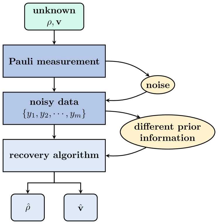
Figure 1: Schematic procedure of the corrupted sensing quantum state tomography. For the unknown state $\rho$ and noise ${\bf v}$, Pauli measurements are employed to get the noisy data ${\bf y}=\{y_{1},y_{2},\cdots,y_{m}\}$. With different prior information, one can choose various recovery algorithms to get the reconstructed state $\hat{\rho}$ and noise $\hat{{\bf v}}$; see Eqs. (4),  (9), and  (10).

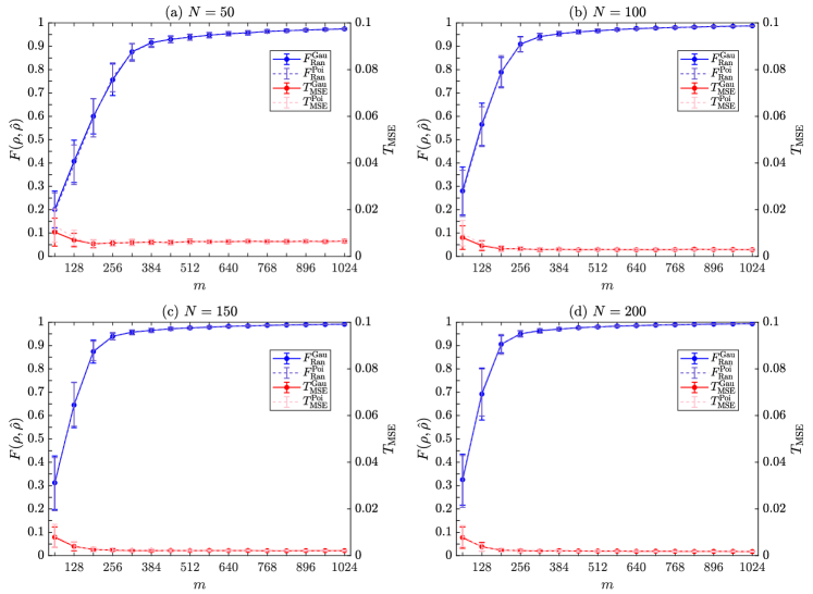
Figure 2: Fidelity $F(\rho,\hat{\rho})$ and MSE $T_{\text{MSE}}$ as functions of the number of sampled Pauli operators $m$ (ranging from $64$ to $1024$ with steps of $64$) over $120$ runs with $n=5$ qubits. The blue solid curve (purple dashed curve) represents the fidelity between the reconstructed state and true state in the case of Gaussian (Poisson) noise. Meanwhile, the red solid curve (pink dashed curve) represents the MSE between the reconstructed Gaussian (Poisson) noise and true Gaussian (Poisson) noise. The number of copies of the input random pure states used for each experiment in (a), (b), (c), and (d) are ${N=50,100,150}$, and $200$, respectively. Standard deviation of the Gaussian noise and parameter of the Poisson noise are both set to ${\sigma=\lambda=4}$. Additionally, the regularization parameters are chosen as ${\tau_{1}=0.011m}$, ${\tau_{2}=0.16}$, and the sparsity level is defined as ${s=\lfloor 0.04m\rfloor}$.

III The corrupted sensing QST algorithm

We consider the general case where the structure of the state and noise can be characterized by a suitable norm function. Typical examples of such structures include low-rank matrices and sparse vectors. Hereafter, let $f(\cdot)$ and $g(\cdot)$ denote the suitable norms which fully characterize the structures of the state and noise respectively.

The reconstruction of the unknown state $\rho$ and structured noise ${\bf v}$ without prior assumptions can be formulated as the following convex optimization problem

$$\underset{\tilde{\rho},\tilde{{\bf v}}}{\text{min}} \frac{1}{2}\|{\bf y}-\mathcal{M}(\tilde{\rho})-\tilde{{\bf v}}\|_{2}^{2}+\tau_{1}\cdot f(\tilde{\rho})+\tau_{2}\cdot g(\tilde{{\bf v}})\,,$$ (4)

where ${\tau_{1},\tau_{2}>0}$ are regularization parameters, and $\tilde{\rho}$ and $\tilde{{\bf v}}$ represent the variables to be solved. The intuition of the problem is to find $\tilde{\rho},\tilde{{\bf v}}$ which fit the data ${\bf y}$ while minimizing the least-squares linear regression with suitable norm regularizations.

Here we consider minimizing the trace norm ${\|X\|_{\mathrm{tr}}=\mathrm{tr}(\sqrt{X^{\dagger}X})}$, which is an alternative to minimizing the rank of $X$ for the quantum state and the $l_{1}$-norm for the sparse noise. Therefore, the estimators $\hat{\rho},\hat{{\bf v}}$ are obtained by

$$(\hat{\rho},\hat{{\bf v}})=\arg\underset{\tilde{\rho}\geq 0,\tilde{{\bf v}}}{\text{min}} \frac{1}{2}\|{\bf y}-\mathcal{M}(\tilde{\rho})-\tilde{{\bf v}}\|_{2}^{2}+\tau_{1}\cdot\|\tilde{\rho}\|_{\mathrm{tr}}$$ (5)

$$+\tau_{2}\cdot\|\tilde{{\bf v}}\|_{1},\tau_{1},\tau_{2}>0\,.$$

Whenever the trace of the resulting estimate of the quantum state is not equal to $1$, we renormalize it as ${\hat{\rho}/\mathrm{tr}(\hat{\rho})\mapsto\hat{\rho}}$. To quantify the goodness of the reconstruction, we employ the (squared) fidelity [34]

$$F(\rho,\hat{\rho})=\left(\mathrm{tr}\sqrt{\sqrt{\hat{\rho}}\rho\sqrt{\hat{\rho}}}\right)^{2}\,,$$ (6)

and the mean squared error (MSE)

$$T_{\text{MSE}}=\frac{1}{m}\sum_{i=1}^{m}({\bf v}_{i}-\hat{{\bf v}}_{i})^{2}\,$$ (7)

for the estimators $\hat{\rho}$ and $\hat{{\bf v}}$ respectively. Note that sometimes we simplify the fidelity $F(\rho,\hat{\rho})$ by $F$.

IV Applications

Using Pauli measurements, we numerically simulate the reconstruction of ${n=5}$ qubit random states and $W$ states under the corruption of $s$-sparse statistical noise. In light of the convex characteristic [36] of our problem in Eq. (5), we rely on the cvx package [37] for efficient numerical solutions.

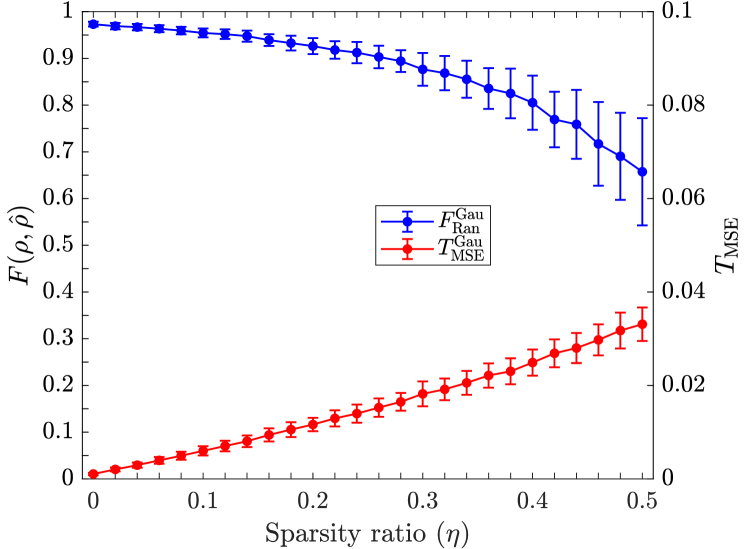
Figure 3: Fidelity $F(\rho,\hat{\rho})$ and MSE $T_{\text{MSE}}$ as functions of the sparsity ratio $\eta$ over $120$ runs with ${n=5}$ qubits. The number of copies of the input random pure states used for each measurement is specified as ${N=100}$, and the number of Pauli operators is fixed as ${m=512}$. Standard deviation of the Gaussian noise is set to ${\sigma=4}$, and the regulation parameters are chosen as ${\tau_{1}=0.011m,\tau_{2}=0.16}$.

IV.1 Corruption by sparse statistical noise

Due to the environment and measurement errors, Gaussian noise is unavoidable in any quantum information processing tasks. Besides, in precision measurement and quantum optics, dark count rate is an important parameter of single-photon detectors which contributes as a main factor leading to error rates in tasks such as quantum communication [38, 39]. Dark count refers to the trigger of a detector in the absence of actual photons, which can usually be modeled as sparse Poisson noise. In experiments, it is desirable to have a low dark count rate. Assuming a Gaussian distribution appropriate for the thermal noise, the expected dark count rate can be reduced to as low as $10^{-3}$ cps [40].

For the first application, we consider random pure states; see Appendix C for the case of $W$ states. Figure 2 displays the fidelity $F(\rho,\hat{\rho})$ and the MSE $T_{\text{MSE}}$ as functions of the number of sampled Pauli operators $m$ (ranging from $64$ to $1024$ with steps of $64$) over $120$ runs. For each Pauli operator $P_{k}$, we take $N$ ($=50,100,150,200$ respectively for the four subfigures) copies of the input random states in order to get the estimated value of $\mathrm{tr}(P_{k}\rho)$. Several features are immediately available.

Under sparse Gaussian noise, the fidelity $F(\rho,\hat{\rho})$ (blue solid curve) improves along with the increasing number of sampled Pauli operators $m$. For instance, in Fig. 2 (b), the fidelity can quickly reach to ${\sim 0.987}$ with ${m=1024}$ and ${N=100}$. Normally, to obtain the fidelity of ${F(\rho,\hat{\rho})\approx 0.95}$, only ${m\approx 37.5\%d^{2}}$ measurements are needed. In addition, a large number of samples prove advantageous in enhancing the precision and stability of the reconstruction. In Fig. 2 (a)-(d) with ${N=50,100,150}$, and $200$, achieving ${F(\rho,\hat{\rho})\approx 0.95}$ necessitates ${m\approx 640,384,320}$, and $256$, respectively.

On the other hand, the MSEs $T_{\text{MSE}}$ between the reconstructed noise and true noise (red solid curve) are all in the order of $10^{-3}$ for Fig. 2 (a)-(d) as long as the fidelity of the corresponding reconstructed state reaches the threshold of $0.95$. Expectedly, the MSE declines and stabilizes as $m$ and $N$ grow.

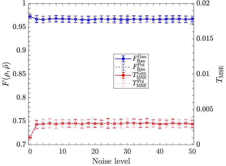
Figure 4: Fidelity $F(\rho,\hat{\rho})$ and MSE $T_{\text{MSE}}$ as functions of standard deviation of the Gaussian noise $\sigma$ and parameter of the Poisson noise $\lambda$ over $120$ runs with ${n=5}$ qubits. The number of copies of the input random pure states used for each measurement is specified as ${N=100}$ and the number of Pauli operator is fixed as ${m=512}$. The regulation parameters are chosen as ${\tau_{1}=0.011m,\tau_{2}=0.16}$. The sparsity level is defined as ${s=\lfloor 0.04m\rfloor}$.

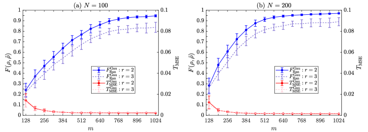
Figure 5: Fidelity $F(\rho,\hat{\rho})$ and MSE $T_{\text{MSE}}$ as functions of the number of sampled Pauli operators $m$ over $120$ runs of the input rank-$2$, rank-$3$ random states with $n=5$ qubits. The copy numbers used for each measurement are as follows: (a) $N=100$, and (b) $N=200$. Standard deviation of the Gaussian noise is set to $\sigma=4$. And the regulation parameters are chosen as $\tau_{1}=0.0055*m,\tau_{2}=0.15$. The sparsity level is defined as $s=\lfloor 0.04m\rfloor$.

Notably, sparse Poisson noise exhibits effects on reconstruction similar to sparse Gaussian noise under specific parameter settings, despite their different probability distributions and statistical characteristics. This reflects the universality of our reconstruction algorithm to statistical noise, providing further insights for selecting appropriate noise models.

Figure 3 displays the fidelity and MSE as functions of the sparsity ratio. Here we consider random pure states with $s$-sparse Gaussian noise, i.e., those with ${s=\lfloor\eta m\rfloor}$ nonzero elements. Correspondingly, the sparsity ratio $\eta$ quantifies the proportion of nonzero elements within the vector ${\bf v}$. It is evident that with the increase of the sparsity ratio $\eta$, the fidelity decreases, accompanied by an escalation in MSE. As the sparse proportion does not exceed $\sim 10\%$, the fidelity ${F(\rho,\hat{\rho})\gtrsim 0.95}$.

There are many factors affecting the setting of regularization parameters $\tau_{1}$ and $\tau_{2}$. Based on empirical observations, one can initially select a few integer values to narrow down the parameter range. Alternatively, intelligent algorithms like the genetic algorithm can be employed to assist in the parameter selection. Here, we choose ${\tau_{1}=0.011m,\tau_{2}=0.16}$, and leave the optimal parameter selection as an open problem.

IV.2 Robustness of the protocol

To demonstrate the algorithm’s robustness, we show the variations in fidelity $F(\rho,\hat{\rho})$ and MSE $T_{\text{MSE}}$ with respect to the noise level of Gaussian and Poisson sparse noise in Fig. 4 by changing the corresponding parameters $\sigma$ and $\lambda$. The results confirm that our protocol remains robust against different noise levels. Specifically, considering sparse Gaussian noise with standard deviation ${\sigma=0}$ as corruption, it results in ${F(\rho,\hat{\rho})\approx 0.97}$ and ${T_{\text{MSE}}\approx 10^{-3}}$ due to systematic error. As $\sigma$ grows, the fidelity consistently stays $\sim 0.96$, with ${T_{\text{MSE}}\approx 3\times 10^{-3}}$. The relative $l_{2}$-norm error of the noise reconstruction is displayed in Appendix D. Consistent with the findings in Fig. 2, the scenarios of the changes in Poisson noise level exhibit similar impacts on fidelity and MSE to those of the Gaussian noise.

In reality, the input state $\rho$ can never be a pure state as affected by any potential noise, resulting in higher-rank states. Using sparse Gaussian noise, Fig. 5 displays fidelity $F(\rho,\hat{\rho})$ and MSE $T_{\text{MSE}}$ as functions of the number of sampled Pauli operators $m$ for rank-2 and rank-3 input random states. For the case of rank-2 random state, employing all available measurement operators yields fidelities reaching up to ${F(\rho,\hat{\rho})\approx 0.947}$ and ${F(\rho,\hat{\rho})\approx 0.97}$, with ${T_{\text{MSE}}\approx 2.3\times 10^{-3}}$ and ${T_{\text{MSE}}\approx 1.5\times 10^{-3}}$ in Fig. 5 (a) and (b), respectively. While for the case of rank-3 random state with ${N=200}$, the fidelity ${F(\rho,\hat{\rho})}$ attains $0.89$ for ${m=1024}$, accompanied by a corresponding MSE ${T_{\text{MSE}}\approx 1.7\times 10^{-3}}$. The regularization parameters $\tau_{1},\tau_{2}$ are fine-tuned here, one can also achieve a higher fidelity by increasing the number of samples.

Furthermore, due to the existence of inevitable systematical noise, we shall consider noise to the state by applying independent and identical depolarizing channels to each of the $n$ qubits. The depolarizing channel with strength $\gamma$ acting on a single qubit $\rho$ is

$$\mathcal{E}(\rho)=\frac{\gamma\openone}{2}+(1-\gamma)\rho\,.$$ (8)

This means that, with probability $\gamma$ the qubit is replaced by a completely mixed state and otherwise it is left untouched. We assume very weak decoherence and set ${\gamma=0.01}$. For input random pure states with $1\%$ local depolarizing noise, Fig. 6 shows the fidelity ${F(\rho,\hat{\rho})}$ between the reconstructed state and the true state, as well as the MSE ${T_{\text{MSE}}}$ of sparse Gaussian noise, plotted as functions of the number of sampled Pauli operators $m$. When all the Pauli operators are employed, the fidelity ${F(\rho,\hat{\rho})\approx 0.936}$ is achieved with ${N=50}$, and the corresponding MSE ${T_{\text{MSE}}\approx 6.5\times 10^{-3}}$. Subsequently, we increase the number of copies, as shown in Fig. 6 (b), resulting in a boosted fidelity of ${F(\rho,\hat{\rho})\approx 0.95}$ and ${T_{\text{MSE}}\approx 2.9\times 10^{-3}}$.

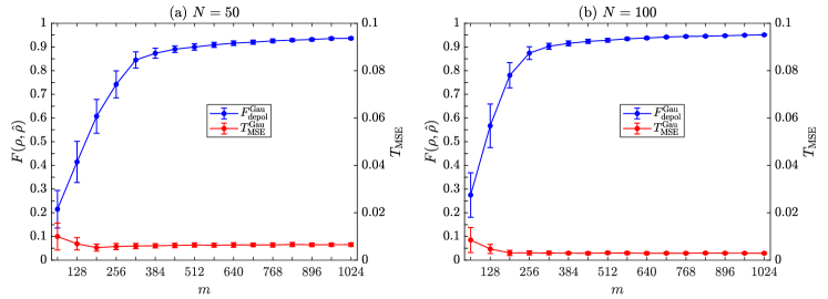
Figure 6: Fidelity $F(\rho,\hat{\rho})$ and MSE $T_{\text{MSE}}$ as functions of the number of sampled Pauli operators $m$ over $120$ runs with $n=5$ qubits. The number of copies of the input random pure states with $1\%$ local depolarizing noise used for each measurement in (a), (b) are specified as ${N=50,100}$ respectively. Standard deviation of the Gaussian noise is set to ${\sigma=4}$. And the regulation parameters are chosen as ${\tau_{1}=0.011m,\tau_{2}=0.16}$. The sparsity level is defined as ${s=\lfloor 0.04m\rfloor}$.

V Summary

In this work, we have proposed a scheme of corrupted sensing quantum state tomography and investigated its application under the assumption of low-rank density matrix and sparse statistical noise. Specifically, extensive numerical simulations were employed to demonstrate the simultaneous tomography performance of five-qubit random pure states under corrupted noise characterized by Gaussian and Poisson sparse noise, respectively. Our findings showed that by utilizing a limited number of quantum states and an incomplete set of measurement operators, the fidelity of the reconstructed state can reach as high as ${F(\rho,\hat{\rho})\gtrsim 0.95}$, and the MSE of the reconstructed noise is found to be in the order of $10^{-3}$. Expectedly, the reconstruction performance can be further improved by increasing the number of input quantum states and measurement operators.

Furthermore, we examined the robustness of the protocol by exploring different levels of the corrupted noise as well as random states with higher ranks. On top of that, we assessed the protocol’s efficacy of the input states with local depolarizing noise. The results showcased the robustness and practicality of the protocol in real-world scenarios, especially for low-rank quantum states and relatively sparse noise. These findings offer valuable insights into the noise diagnosis and characterization of quantum systems.

We would like to highlight several interesting potential directions to explore in future. Firstly, we stress that the success of the algorithm is contingent on that proper values of the free parameters $\tau_{1},\tau_{2}$ can be found, and what are the optimal parameters is left as an open problem. Secondly, the simple cvx tool was employed as the initial solution for the protocol, while future work can explore more advanced techniques. Lastly, it is also essential to consider more diverse and intricate types of noise beyond statistical noise.

On the theoretical side, it would be necessary to derive a tight lower bound for the number of measurements required for the successful reconstruction of the quantum state and corrupted noise simultaneously. Instead of using restricted isometry property tools to assess random Pauli measurements as in compressed sensing, the use of extended matrix deviation inequality may be explored to build the extended measurement matrix [32]. Furthermore, a concrete analysis of the error bound is warranted to provide insights into the algorithm’s robustness and limitations. This would involve investigating the maximal tolerable noise levels and evaluating the algorithm’s performance near critical thresholds.

Appendix A The constrained setting

When prior knowledge of the corrupted noise ${\bf v}$ (in terms of the $l_{1}$-norm) and the noise strength $\delta$ (in terms of the $l_{2}$-norm) of the unstructured noise ${\bf z}$ are available, we can consider the following constrained convex recovery algorithm

$$\underset{\tilde{\rho}\geq 0,\tilde{{\bf v}}}{\text{min}}\quad \|\tilde{\rho}\|_{\mathrm{tr}}\,,$$ (9)

s.t. $$\|\tilde{{\bf v}}\|_{1}\leq\beta\cdot\|{\bf v}\|_{1},\|{\bf y}-\mathcal{M}(\tilde{\rho})-\tilde{{\bf v}}\|_{2}\leq\delta,\beta>0\,.$$

For data collection, we may generate a Gaussian noise vector ${\bf z}$ and scale it such that ${\|{\bf z}\|_{2}=\delta}$.

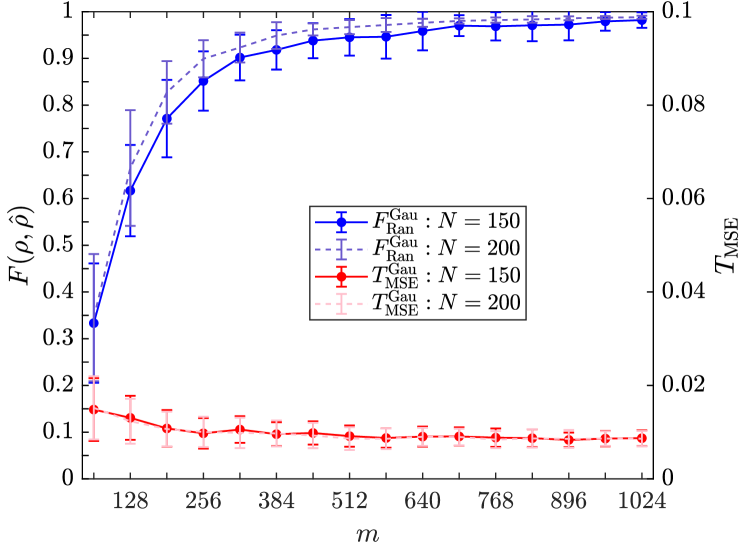
Figure 7: Fidelity $F(\rho,\hat{\rho})$ and MSE $T_{\text{MSE}}$ as functions of the number of sampled Pauli operators $m$ over $120$ runs with $n=5$ qubits, when prior knowledge of the corrupted noise and the noise strength $\delta$ of ${\bf z}$ are available. The input pure states are chosen randomly and the standard deviation of the corrupted Gaussian noise is set to ${\sigma=4}$. The sparsity level is set to ${s=\lfloor 0.05m\rfloor}$. Other parameters are chosen as ${\beta=1.42}$ and ${\delta=0.1}$.

In Fig. 7, with ${N=150}$ state copies, fidelity of the reconstructed state can reach $0.95$ for ${m=640}$ measurement operators, and it can be further increased to ${F(\rho,\hat{\rho})\approx 0.982}$ by using the complete set of measurement operators. The corresponding MSEs for both cases are ${T_{\text{MSE}}\approx 9\times 10^{-3}}$. Upon increasing the number of copies to $N=200$, a fidelity of $0.96$ is achieved with ${m=448}$ operators, and ${F(\rho,\hat{\rho})\approx 0.988}$ with the complete set of measurement operators. The MSE is comparable to the case of ${N=150}$. By the same token, one can also consider the scenario when prior knowledge of the quantum state and noise strength of the unstructured noise are known to minimize the $l_{1}$-norm of the corrupted noise.

Appendix B The penalized setting

When only the noise strength $\delta$ of the unstructured noise is known, it is convenient to use the following penalized convex recovery algorithm

$$\underset{\tilde{\rho}\geq 0,\tilde{{\bf v}}}{\text{min}}\quad \lambda_{1}\cdot\|\tilde{\rho}\|_{\mathrm{tr}}+\lambda_{2}\cdot\|\tilde{{\bf v}}\|_{1}\,,$$ (10)

s.t. $$\|{\bf y}-\mathcal{M}(\tilde{\rho})-\tilde{{\bf v}}\|_{2}\leq\delta,\lambda_{1},\lambda_{2}>0\,.$$

The results are shown in Fig. 8. To a certain extent, there is another trade-off between the accuracy of the state reconstruction and precision of the structured noise recovery, which can be evaluated by choosing the free parameters $\lambda_{1}$ and $\lambda_{2}$. The findings reveal that for the case of ${N=150}$, when the fidelity reaches ${\sim 0.96}$, the number of measurement operators to be used is ${m\sim 640}$. And a fidelity of ${F(\rho,\hat{\rho})\approx 0.99}$ can be reached by increasing the state copies to ${N=300}$. Meanwhile, all MSEs are in the order of $10^{-3}$.

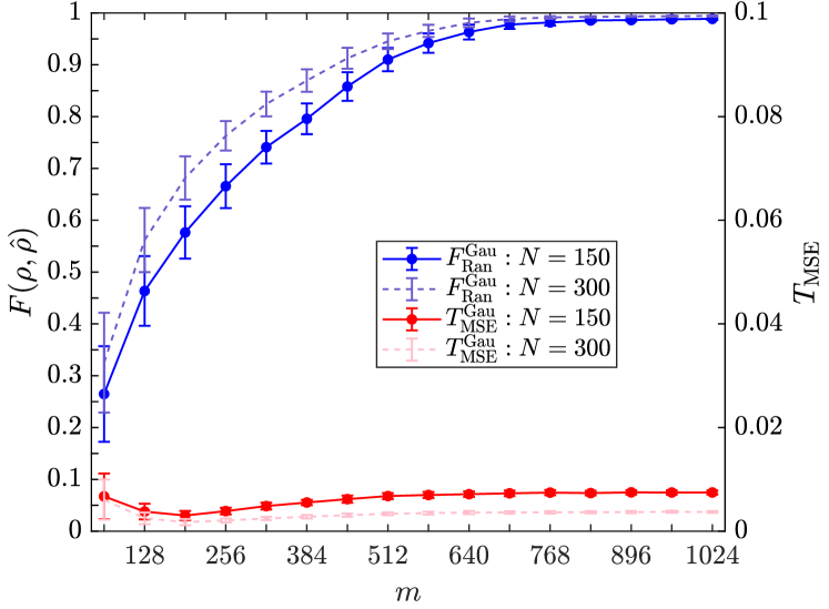
Figure 8: Fidelity $F(\rho,\hat{\rho})$ and MSE $T_{\text{MSE}}$ as functions of the number of sampled Pauli operators $m$ over $120$ runs with ${n=5}$ qubits, when prior knowledge of the noise strength $\delta$ of ${\bf z}$ is available. The input pure states are chosen randomly and the standard deviation of the corrupted Gaussian noise is set to ${\sigma=4}$. The sparsity level is defined as ${s=\lfloor 0.04m\rfloor}$. The regulation parameters are chosen as ${\lambda_{1}=0.001m,\lambda_{2}=0.014+0.002\cdot\frac{m-64}{m}}$, and ${\delta=0.1}$.

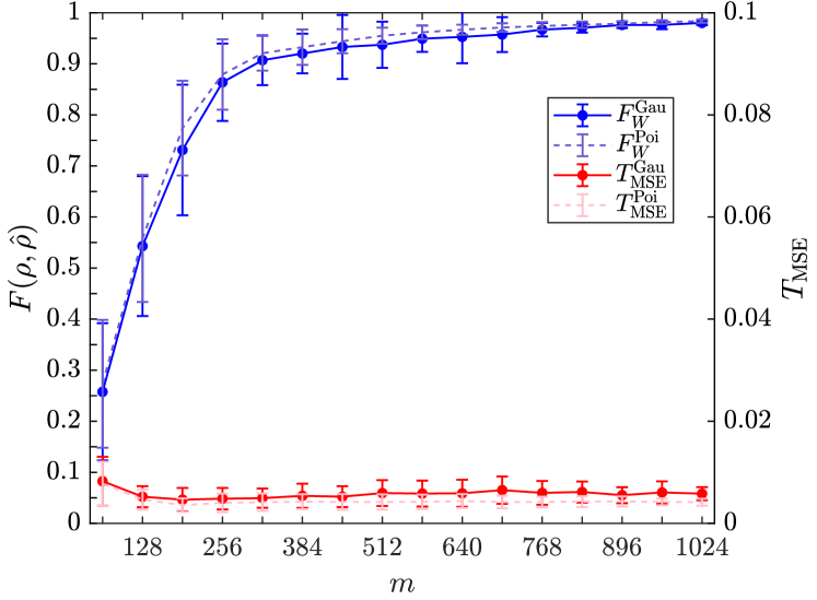
Figure 9: Fidelity $F(\rho,\hat{\rho})$ and MSE $T_{\text{MSE}}$ as functions of the number of sampled Pauli operators $m$ for five-qubit $W$ state over $120$ runs. The number of copies used for each measurement is specified as ${N=100}$. The regulation parameters are chosen as ${\tau_{1}=0.011m,\tau_{2}=0.16}$. Standard deviation of the Gaussian noise and parameter of the Poisson noise are set to ${\sigma=\lambda=4}$. The sparsity level is defined as ${s=\lfloor 0.04m\rfloor}$.

Appendix C $W$ state with corruption

A similar simulation experiment is performed to test the $W$ state for a five-qubit system with corruption. An $n$-qubit $W$ state is written as

$$\mbox{$|W_{n}\rangle$}=\frac{1}{\sqrt{n}}(\mbox{$|10\cdots 0\rangle$}+\mbox{$|01\cdots 0\rangle$}+\mbox{$|00\cdots 1\rangle$})\,.$$ (11)

As can be seen in Fig. 9, variations of the fidelity and MSE are similar to those of the random pure states. Using the same parameter settings with Gaussian noise, when ${N=100}$, the number of measurements required to achieve a fidelity of $0.95$ is about ${m=640}$ and the corresponding MSE is ${T_{\text{MSE}}\approx 6\times 10^{-3}}$. Moreover, the fidelity can reach as high as ${F(\rho,\hat{\rho})=0.98}$ when ${m=1024}$. In addition, it is worth mentioning that the parameter selection here may not be optimal, as the parameters can be adjusted depending on the scenarios being tested.

Appendix D Recovery noise error

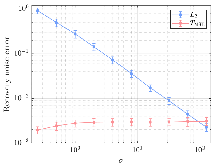
Figure 10: Relative $l_{2}$-norm error $L_{2}$ and MSE ${T_{\text{MSE}}}$ as functions of the standard deviation of the Gaussian noise $\sigma$ over $120$ runs with ${n=5}$ qubits. The number of copies of the input random pure states used for each measurement is specified as ${N=100}$ and the number of Pauli operators is fixed as ${m=512}$. The regulation parameters are chosen as ${\tau_{1}=0.011m,\tau_{2}=0.16}$. The sparsity level is defined as ${s=\lfloor 0.04m\rfloor}$.

We define the relative $l_{2}$-norm error $L_{2}$ as

$$L_{2}=\frac{\|\hat{{\bf v}}-{\bf v}\|_{2}}{\|{\bf v}\|_{2}}\,.$$ (12)

Figure 10 shows the recovery noise error measured by $L_{2}$ and ${T_{\text{MSE}}}$ as functions of the standard deviation of the Gaussian noise. The standard deviation $\sigma$ is varied within the range ${[2^{-2},2^{7}]}$, increasing by the powers of $2$. The relative $l_{2}$-norm error decreases from ${L_{2}\approx 0.92}$ to ${L_{2}\approx 2.3\times 10^{-3}}$.