Graphcode: Learning from multiparameter persistent homology using graph neural networks
Abstract
We introduce graphcodes, a novel multi-scale summary of the topological properties of a dataset that is based on the well-established theory of persistent homology. Graphcodes handle datasets that are filtered along two real-valued scale parameters. Such multi-parameter topological summaries are usually based on complicated theoretical foundations and difficult to compute; in contrast, graphcodes yield an informative and interpretable summary and can be computed as efficient as one-parameter summaries. Moreover, a graphcode is simply an embedded graph and can therefore be readily integrated in machine learning pipelines using graph neural networks. We describe such a pipeline and demonstrate that graphcodes achieve better classification accuracy than state-of-the-art approaches on various datasets.
1 Introduction
A quote attributed to Gunnar Carlsson says "Data has shape and shape has meaning". Topological data analysis (TDA) is concerned with studying the shape, or more precisely the topological and geometric properties of data. One of the most prominent tools to quantify and extract topological and geometric information from a dataset is persistent homology. The idea is to represent a dataset on multiple scales through a nested sequence of spaces, usually simplicial complexes for computations, and to measure how topological features like connected components, holes or voids appear and disappear when traversing that nested sequence. This information can succinctly be represented through a barcode, or equivalently a persistence diagram, which capture for every topological feature its lifetime along the scale axis. Persistent homology has been successfully applied in a wealth of application areas [13, 22, 27, 29, 30, 35], often in combination with Machine Learning methods – see the recent survey [21] for a comprehensive overview.
A shortcoming of classical persistent homology is that it is bound to a single parameter, whereas data often is represented along several independent scale axes (e.g., think of RGB images which have three color channels along which the image can be considered). To get a barcode, one is forced to chose fixed scales for all but one scale parameters. The extension to multi-parameter persistent homology [6, 8] avoids to make such choices. Similar to the one-parameter setup, the data is represented in a nested multi-dimensional grid of spaces and the evolution of topological features in this grid is analyzed. Unfortunately, a succinct representation as a barcode is not possible in this extension, which makes the theory and algorithmic treatment more involved. Nevertheless, the quest of how to use informative summaries in multi-parameter persistence is an active field of contemporary research. A common theme in this context is vectorization, meaning that some (partial) topological information is extracted from the dataset and transformed into a high-dimensional vector suitable for machine learning pipelines.
Contribution.
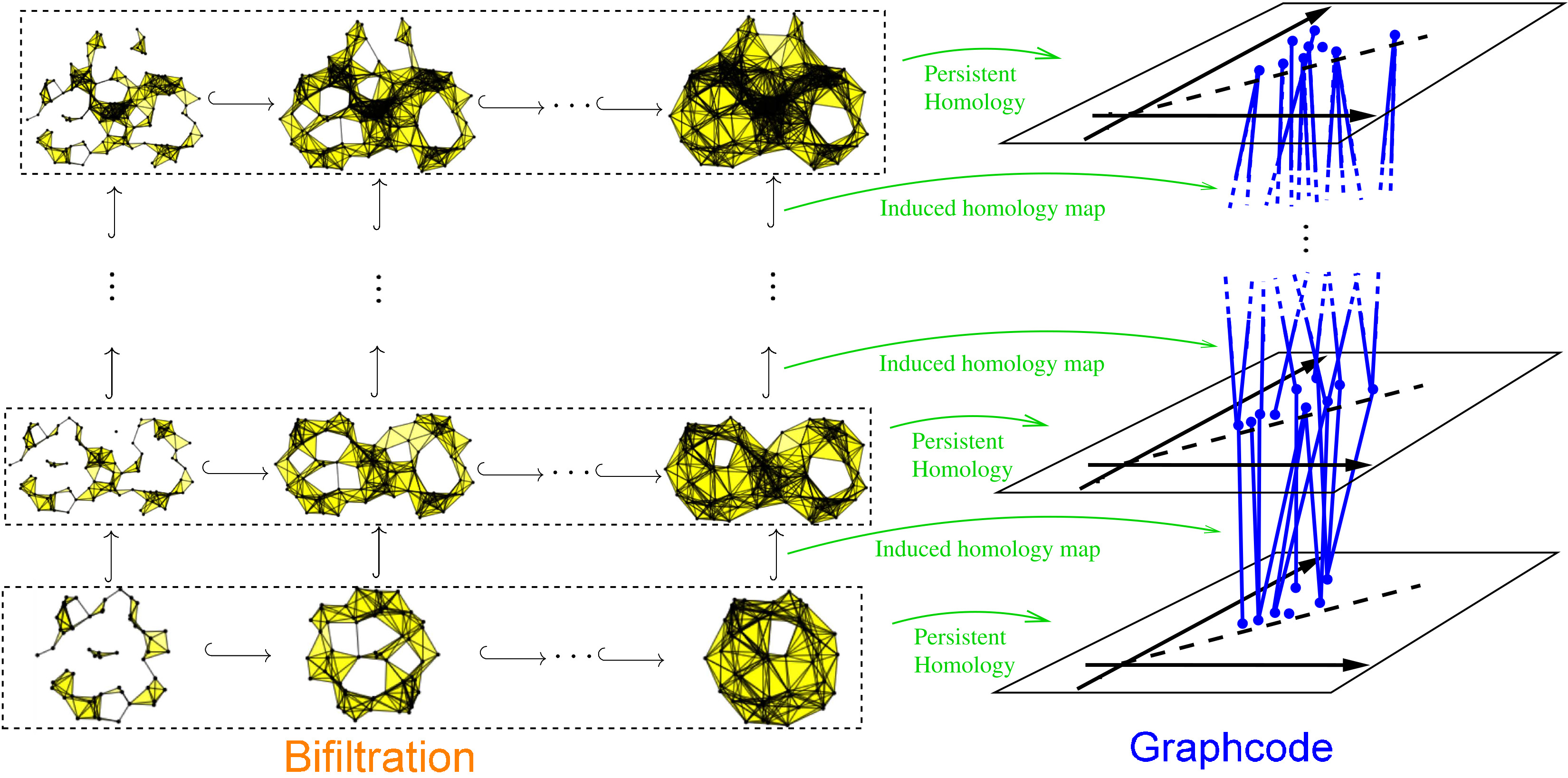
We introduce graphcodes, a novel representation of the homology of a dataset that is filtered along two scale parameters. The idea, depicted in Figure 1, is to consider one-parameter slices of the dataset by fixing one parameter, obtaining a stack of persistence diagrams. We define a map between two consecutive diagrams in this stack, resulting in a bipartite graph connecting these diagrams. The graphcode is the union of these bipartite graphs over all consecutive pairs.
Since the maps connecting diagrams depend on a choice of basis for each persistence diagram, the graphcode is not a topological invariant. Nevertheless, the graphcode is a combinatorial description whose features are easy to interpret and which permits, for fixed bases per diagram, a complete reconstruction of the persistence module induced by the bifiltration. Moreover, the structure as an (embedded) graph in admits a direct integration of graphcodes into machine learning pipelines via graph neural network architectures. In that way, graphcodes avoid the vectorization step of other homology-enhanced learning pipelines which often require more parameter choices and are sometimes slow in practice. In contrast, we describe an efficient algorithm to compute the graphcode of a bifiltered simplicial complex which essentially computes all required information through a single out-of-order matrix reduction of the boundary matrix of the entire complex. While the worst-case complexity is cubic, the practical performance is closer to linear for realistic datasets [4, 28].
We demonstrate how graphcodes facilitate classification tasks. For that, we implemented a machine learning pipeline that feeds the graphcodes into a simple graph neural network pipeline. On graph datasets used in related works on multi-parameter persistent learning, our approach shows a comparable classification quality. As a proof of concept, we also created a synthesized dataset of point clouds in that contain a number of densely sampled disks and annuli plus some uniform noise. Clearly, topological classifiers are well-suited for such data. In our experiments, graphcodes outperform related methods on this type of data in terms of accuracy. At the same time, graphcodes are faster computed than all alternative topological descriptors, sometimes by several orders of magnitude. We also demonstrate that graphcodes perform better than other topological methods on two further datasets, established in related work on TDA, which consist of samples from different random point processes and orbits generated by a dynamical system, respectively.
Related work.
Our method can be viewed as a generalization of PersLay [10] to the two-parameter case. PersLay is a neural network layer that enables vectorization-free learning from one-parameter persistent homology. It uses a deep set [36] architecture to directly take persistence diagrams as input. A conceptually simpler generalization of PersLay would consist of only using the union of persistence diagrams of the one-parameter slices, that is, the graphcode without connecting edges. We show in our experiments, however, that the edges improve the accuracy in the two-parameter case.
Most of the previous methods used in applications are based on transforming persistence diagrams into vectors in Euclidian space, or other data structures suitable for machine learning. Examples are persistence landscapes [7], persistence images [1], or scale-space kernels [31]. These vectorization methods for one-parameter persistence modules have been generalized in various forms to the two-parameter case [9, 15, 17, 25, 34]. The difference in the two-parameter case is that the vectorizations are not based on a complete invariant like the persistence diagram but on weaker invariants like the rank-invariant, generalized rank-invariant or the signed barcode. Hence, these vectorizations capture the persistent homology only partially. Moreover, even this partial information is often times computationally expensive. In contrast, our method avoids to compute a direct vectorization, although we point out that a vectorization is implicitly computed eventually within the graph neural network architecture. To our knowledge there exists no other method that allows to feed a complete representation of two-parameter persistent homology into a machine learning pipeline.
Our approach also resembles persistent vineyards [16] in the sense that a two-parameter process is considered as a dynamic -parameter process and the evolution of persistence diagrams is analyzed. Indeed, vineyards produce a layered graph of persistence diagrams just as graphcodes (see Fig VIII.6 in [18]), but they operate in a different setting where the simplicial complex is fixed throughout the process and only the order of simplices changes, whereas graphcodes rely on bifiltered simplicial complex data that only increases along both axis. Most standard constructions of multi-parameter persistence yield such a bifiltered complex and graphcodes are more applicable in this situation.
Generating bifiltered simplicial complexes out of point cloud data is computationally expensive and an active area of research. In the context of the aforementioned two-dimensional point clouds that we analyze with graphcodes, we heavily rely on sublevel Delaunay bifiltrations which were introduced very recently by Alonso et al. [2]. That algorithm (and its implementation) render the two-parameter analysis of such point clouds possible in machine learning contexts, partially explaining why previous methods have only tested their approaches on very small point cloud data, if at all.
Outline.
We review basic notions of persistent homology in Section 2 and define graphcodes in Section 3 based on these definitions. We decided for a “down-to-earth” approach, defining graphcodes in terms of cycle bases in simplicial complexes to keep concepts concrete and relatable to geometric constructions for the benefit of readers that are not too familiar with the algebraic foundations of persistent homology. Moreover, this treatment simplifies the algorithmic description to compute graphcodes in Section 4. We explain the machine learning architecture based on graphcodes in Section 5 and report on our experimental results in Section 6. We conclude in Section 7.
2 Persistent homology
We will use the following standard notions from simplicial homology. For readers not familar with these concepts, we provide a summary in Appendix A. For a more in-depth treatment see, for instance, the textbook by Edelsbrunner and Harer [18].
For an (abstract) simplicial complex and an integer, let denote its -th chain group with coefficients (which is, in fact, a vector space) and the boundary map (see also Figure 2 (left)). Let be the kernel of . Elements of are called -cycles. is the image of , and its elements are called -boundaries. The quotient is called the -th homology group , whose elements are denoted by with a -cycle, or just if the underlying complex is clear from context. See Figure 2 (right) for an illustration of these concepts.
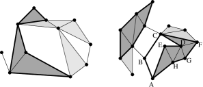
Right: The -cycle marked in thick on the left is also a -boundary, since it is the image of the boundary operator under the marked -simplices. On the right, the -cycle going along the path is not a -boundary; therefore it is a generator of an homology class of . Likewise, the -cycle going along is not a -boundary neither. Furthermore, since the sum is the -cycle given by the path , which is a -boundary because of the marked -simplices. Hence, and represent the same homology class which is characterized by looping aroung the same hole in .
We call a basis of (boundary-)consistent if there exists some such that is a basis of . In this case, is a basis of . A consistent basis can be obtained by first determining a basis of and completing it to a basis of . Clearly, usually has many consistent bases.
Homology maps.
Let be a subcomplex. The inclusion map from to maps -cycles of to -cycles of and -boundaries of to -boundaries of . It follows that for every , the map is a well-defined map between homology groups. This map is a major object of study in topological data analysis, as it contains the information how the topological features (i.e., the homology classes) evolve when we embed them on a larger scale (i.e., a larger complex).
Being a linear map, can be represented as a matrix with -coefficients. It is instructive to think about how to create this matrix: Assuming having fixed consistent bases for and for and considering a basis element of , we write the -cycle as a linear combination with respect to the basis . We can ignore summands that correspond to basis elements of , and the remaining entries yield the image of in , and thus one column of the matrix of .
Alternatively, takes a diagonal form when picking suitable consistent bases and . We can do that as follows: We start with a basis of , the set of -cycles in that become “trivial” when included in . This subspace contains and we can choose such that it starts with a basis of , followed by other vectors. Now we extend to a basis of which is consistent by the choice of . Since is a subspace of , we can extend to a basis of . Importantly, we can do so such that is consistent, because the sub-basis maps to and does not, so we can first extend to a basis of , ensuring consistency, and then extend to a full bais of . In this way, considering a homology class with a basis element of , is also a basis element of , and the map indeed takes diagonal form.
Filtrations and barcodes.
A filtration of a simplicial complex is a nested sequence of subcomplexes of . Applying homology, we obtain vector spaces and linear maps whenever . This data is called a persistence module. For simplicity, we assume that is the trivial vector space, implying that all -cycles eventually become -boundaries.
It is possible to iterate the above construction for a single inclusion to obtain consistent bases for such that all maps have diagonal form. Equivalently, there is one basis of that contains consistent bases for all subcomplexes . To make this precise, we first observe that for every , there is a minimal such that for all . This is called the birth index of . Moreover, there is a minimal such that for all . This is called the death index of . By our simplifying assumptions that is trivial, every indeed has a well-defined finite death index. The half-open interval consisting of birth and death index is called the bar of . We say that is already born at index if its birth index is at most . We call alive at if alpha is already born at and is strictly smaller than the death index of ; otherwise we call it dead at .
Definition 2.1.
For a filtration of as above, a barcode basis is a basis of where each basis element is attached its bar such that the following property holds: For every , the elements of dead at form a basis of , and the elements of already born at form a basis of . In particular, these cycles form a consistent basis of .
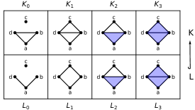
Right: Choosing the basis , for and and for , we have , hence the cycle has two outgoing edges, to both basis elements in . We ignore the basis vector of in the figure, since its birth and death index coincide, so the corresponding feature has persistence zero.
See Figure 3 (left) for an illustration. The collection of bars of a barcode basis is called the barcode of . Indeed, while there is no unique barcode basis for , they all give rise to the same barcode. This barcode (or the equivalent persistence diagram, where a bar is interpreted as a point in the plane) yields a topological summary of the filtration, revealing what topological features are active on which ranges of scale. Therefore, barcodes are a suitable (discrete) proxy for a dataset and are heavily used in applications.
The concept of a barcode basis enhances the barcode with a consistent choice of representative cycle for every bar. In practice, this extra information is obtained with no additional computation costs because the standard algorithm to compute barcodes computes a barcode basis as a by-product.
3 Graphcodes
We now consider the case of two filtered complexes , such that for all :
| (1) |
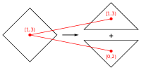
Assume we have fixed barcode bases for and for . The inclusion induces a linear map , mapping each element of to a linear combination of with -coefficients, or equivalently, to a subset of . The map can be represented as a bipartite graph over . By furthermore replacing elements of and with their attached bars, we can interpret this graph as a graph between barcodes, which we call the graphcode of (1). See Figure 3 (right) for an illustration. We emphasize that the graphcode depends on the chosen barcode bases for and , thus the graphcode is not unique, and not a topological invariant.
The bases and together with their graphcode are sufficient to recover the homology maps , induced by the inclusion : Since a basis of is contained in , restricts to a map , and it is not hard to see that this map equals the map induced by the inclusion . Moreover, the basis of within is simply determined by those elements in that are already born at , by definition of the barcode basis. Within this basis, the homology class represented by cycles alive at form a basis of . The image of these classes under yields a linear combination of cycles in which are all already born, and removing the summands corresponding to dead cycles yields the image of in .
Bifiltrations.
Assume our data is now a bifiltered simplicial complex written as
| (2) |
Such a structure often times appears in applications where a dataset is analyzed through two different scales. An example is hierarchical clustering where the points are additionally filtered by an independent importance value.
We can iterate the idea from the last paragraph to a bifiltration in a straight-forward manner: Let be a barcode basis for the horizontal filtration With that bases fixed, there is a graphcode between the -th and -th horizonal filtration, and we define the union of these graphs as the graphcode of the bifiltration. The vertices of the graphcode are bars of the form that are attached to a basis , and we can naturally draw the graphcode in by mapping the vertex to . This yields a layered graph in with respect to the 3rd coordinate with edges only occurring between two consecutive layers. As discussed in Appendix D, graphcodes can be defined for arbitary two-parameter persistence modules. They can also be defined for arbitrary fields, in which case we obtain a graph that has not only node but also edge attributes.
4 Computation
The vertices and edges of a graphcode in homology dimension can be computed efficiently in time where is the total number of simplices of dimension or . We expose the full algorithm in Appendix B in a self-contained way and only sketch the main ideas here for brevity.
First of all, it can be readily observed that the standard algorithm to compute persistence diagrams via matrix reduction yields a barcode basis in time (see [18]). Doing so for every horizontal slice in (2) yields the vertices of the graphcode, and computing the edges between two consecutive slices can be reduced to solving a linear system via matrix reduction as well, resulting in time as well for any two consecutive slices. This is not optimal though as it results in a total running time of with the number of horizontal slices.
To reduce further to cubic time, we perform an out-of-order matrix reduction, where the -simplices are sorted with respect to their horizontal filtration value, but are added to the boundary matrix in the order of their vertical value. This reduction process, which still results in cubic runtime, yields a sequence of snapshots of reduced matrices that correspond to the barcode basis on every horizontal slice, and thus yields all vertices of the graphcode. The final observation is that with additional book-keeping when going from one snapshot to the next, we can track how the basis elements transform from one horizontal slice to the next and these changes encode which edges are present in the graphcode.
Finally, the practical performance can be further improved by reducing the size of the graphcode, by keeping small, by ignoring bars whose persistence is below a certain threshold, and by precomputing a minimal presentation instead of working with the simplicial input. See Appendix B for details.
5 Learning from graphcodes using graph neural networks
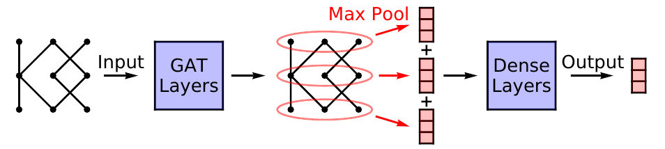
We describe our pipeline that exemplifies how graphcodes can be used in combination with graph neural networks (GNN’s). The inputs are layered graphs with vertex attributes , with a bar of the barcode at the -th layer. We can add further meaningful attributes like the additive and/or multiplicative persistence to the nodes to suggest the GNN that these might be important. Any graph neural network architecture can be used to learn from these topological summaries. We propose the architecture depicted in Figure 4. It starts with a sequence of graph attention (GAT) layers [33] taking the graphcodes as input. The idea is that the network should learn to pay more attention to adjacent features with high persistence which are commonly interpreted as the topological signal. These layers are followed by a local max-pooling layer that performs max-pooling over all vertices in a common slice. Then we concatenate the vectors obtained from the local max-pooling over all slices and feed the resulting vector into a standard feed-forward neural network (Dense Layers).
If we remove all the edges from the graphcodes, this model can be viewed as a combination of multiple Perslay architectures [10], one for each slice of the bifiltration. In such a case, the model would implicitly learn for each barcode individually which bars are important for classification. Adding the edges, in turn, enhances this model as propagation between neighboring layers is possible: a bar that is connected to important bars in adjacent layers is more likely to be significant itself.
We also point out that the separate pooling by slices is crucial in our approach. It takes advantage of the additional information provided by the position of a slice in the graphcode. If we simply embed the entire graphcode in the plane by superimposing all persistence diagrams and do one global pooling, the outcome gets significantly worse.
6 Experiments
We have implemented the computation of graphcodes in a dedicated C++ library and the machine learning pipeline in Python. All the code for our experiments is available in the supplementary materials. The experiments were performed on an Ubuntu 23.04 workstation with NVIDIA GeForce RTX 3060 GPU and Intel Core i5-6600K CPU.
Graph datasets.
We perform a series of experiments on graph classification, using a sample of TUDatasets, a collection of graph instances [26]. Following the approach in [9], we produce a bifiltration of graphs using the Heat Kernel Signature-Ricci Curvature bifiltration. From these bifiltrations, we compute the graphcodes (GC) and train a graph neural network as described in Section 5 to classify them. More details on these experiments can be found in Appendix C.1 and the supplementary materials. We compare the accuracy with multi-parameter persistence images (MP-I) [9], multi-parameter persistence kernels (MP-K) [17], multi-parameter persistence landsacapes (MP-L) [34], generalized rank invariant landscapes (GRIL) [15] and multi-parameter Hilbert signed measure convolutions (MP-HSM-C) [25]. All these approaches produce a vector and use XGBoost [14] to train a classifier.
The results in Table 1 indicate that graphcodes are competitive on these datasets in terms of accuracy. In terms of runtime performance, the instances are rather small and all approaches terminate within a few seconds (with the exception of GRIL that took longer). Also, while the numbers in Table 1 for the previous approaches are taken from [25], we have partially rerun the classification using convolutional neural networks instead of XGBoost. Since the results were comparable, we decided to use the numbers from the previous work.
We remark that we included this test primarily because it is the standard test in related work. Still, it seems unclear that the datasets really have a strong topological signal and it seems also unclear that the learned model really selects a topological feature for its classification, despite the topology-aware design of the methods. Moreover, we believe that the performance of our pipeline relative to the other methods is worse on these datasets compared to the following experiments because the training sets are rather small which is disadvantageous for our GNN architecture.
| Dataset | MP-I | MP-K | MP-L | GRIL | MP-HSM-C | GC |
|---|---|---|---|---|---|---|
| PROTEINS | 67.33.5 | 67.53.1 | 65.83.3 | 70.93.1 | 74.62.1 | 73.62.6 |
| DHFR | 80.22.2 | 81.71.9 | 79.52.3 | 77.62.5 | 81.92.5 | 76.43.9 |
| COX2 | 77.92.7 | 79.91.8 | 79.03.3 | 79.82.9 | 77.13.0 | 78.74.9 |
| MUTAG | 85.67.3 | 86.15.2 | 84.06.8 | 87.84.2 | 85.65.3 | 86.46.1 |
| IMBD-BINARY | 71.12.1 | 68.21.2 | 71.22.0 | 65.22.6 | 74.82.5 | 65.42.7 |
Shape dataset.
To demonstrate that graphcodes are powerful topological descriptors, we apply them on a synthetic shape dataset with a strong topological signal. We construct 5 classes of shapes as follows: Class consists of annuli and disks in the plane. The centers and radii are sampled uniformly such that the shapes do not overlap. This implies that the homology of class in degree one has rank . Now we uniformly sample points from these shapes and add uniform noise. The Figure on the left shows an example of class .
![[Uncaptioned image]](/html/2405.14302/assets/points_5classes.png)
We generate random shape configurations and point samples per class to obtain a dataset of point clouds. The point clouds are labeled with the homology of the underlying shape configuration. The goal is to classify the point clouds according to their homology in degree one. To filter the homology signal from the noise, we first compute a local density estimate at each point in a point cloud and compute the Delaunay-bifiltration [2] with respect to relative density scores. This yields a dataset of labeled bifiltrations. From these bifiltrations, we compute the graphcodes as well as the topological descriptors for the same related approaches as for the graph case. Additionally we also compute one-parameter persistence images (P-I) based on a one-parameter alpha filtration.
The time to compute these topological descriptors is reported in Table 2. Graphcode is faster than every other method, in some cases by orders of magnitude. On the other hand, training graph neural networks is more time-consuming than for convolutional neural networks, and thus graphcodes require more time in the subsequent training phase. In our experiments, the training took around 9 minutes for graphcodes and around 1 minute for other methods.
We now split the various datasets of topological descriptors and class labels into a training set and a test set without labels, train neural networks on the training sets and test their ability to make predictions on the test sets. Further details on these experiments can be found in Appendix C.2 and the supplementary materials. The results in Table 2 show that on this inherently topological classification task, graphcodes outperform every other method by a significant margin. To demonstrate that the graphcode edges that connect consecutive layers add significant information, we run the same experiment on graphcodes with edges removed (GC-NE). The results show even without edges, graphcodes yield a better accuracy compared to related approaches, but also that the edge information further improves accuracy.
| MP-I | MP-L | P-I | GRIL | MP-HSM-C | GC | GC-NE | |
|---|---|---|---|---|---|---|---|
| Accuracy | 64.14.7 | 37.21.5 | 43.62.2 | 74.92.7 | 57.02.3 | 86.91.4 | 82.81.9 |
| Time | 9176 | 3519 | 1090 | 333187 | 282 | 95 | – |
Random point process dataset. The following is a variation of an experiment proposed in [5]: they consider 4 types of random point processes, namely a Poisson, Matérn, Strauss and Baddeley-Silverman process, and try to discriminate the Poisson null model from the other processes using a hypothesis test based on multiparameter persistent Betti numbers. The latter 3 processes are prototypical models for attractive behaviour, repulsive behaviour and complex interactions, respectively. We instead use multiparameter topological descriptors and neural networks to classify these processes. We create a dataset Processes consisting of 4 classes, each of which consisting of point clouds sampled from the above processes and use the topological descriptors and neural networks, discussed for the shape dataset above, for the classification. More details can be found in C.3. The results reported in Table 3 show again that graphcodes outperform other topological descriptors. They also show that for these random point processes the influence of the edges of the graphcodes is much smaller than for the shape dataset. This is expected since prominent persistent features along the density direction are very unlikely in random point processes.
| Dataset | MP-I | MP-L | P-I | GRIL | MP-HSM-C | GC | GC-NE |
|---|---|---|---|---|---|---|---|
| Processes | 66.02.5 | 50.23.0 | 35.510.4 | 61.11.6 | 70.74.9 | 83.42.5 | 83.13.7 |
Orbit dataset. Finally we test our pipeline on another dataset which has been established in topological data analysis as a benchmark in the one-parameter setting. The purpose of this experiment is twofold: On the one hand it demonstrates that grapohcodes can be applied to very big datasets. On the other hand it compares the two-parameter graphcode pipeline to its one-parameter analog PersLay [10]. The dataset consists of orbits generated by a dynamical system defined by the following rule:
| (3) |
where the starting point is sampled uniformly in . The behaviour of this dynamical system heavily depends on the parameter . Following [10], we create two datasets consisting of 5 classes of orbits of points generated by this dynamical system, where the 5 classes correspond to the following five choices of the parameter , , , and . The datasets Orbit5k and Orbit100k consist of and orbits per class, respectively. We again use our graphcode pipeline, discussed for the shape dataset, to classify them. The computation of the graphcodes of the point clouds took just 27 minutes demonstrating the efficiency of our algorithm. The results are reported in Table 4 where we compare them to the results achieved by Persistence Scale Space Kernel (PSS-K) [31], Persistence Weighted Gaussian Kernel (PWG-K) [23], Sliced Wasserstein Kernel (SW-K) [11], Persistence Fisher Kernel (PF-K) [24] and (PersLAY) [10] as reported in Table 1 of [10]. The results demonstrate that graphcodes perform better than the one-parameter methods and underpin our conjecture that the performance of the graphcode-GNN pipeline relative to other methods gets better as the size of the dataset increases. More details can be found in C.4.
| Dataset | PSS-K | PWG-K | SW-K | PF-K | PersLAY | GC | GC-NE |
|---|---|---|---|---|---|---|---|
| Orbit5k | 72.42.4 | 76.60.7 | 83.60.9 | 85.90.8 | 87.71.0 | 88.51.1 | 88.41.5 |
| Orbit100k | - | - | - | - | 89.20.3 | 92.30.3 | 91.50.3 |
7 Conclusion
Our shape experiment shows that current implementations of topological classifiers struggle with simple datasets that contain a clear topological signal but also a lot of noise. A possible explanation is that the vectorization step in these methods blurs the features too much or relies on invariants which might be too weak for a classifier to pick up delicate details. Graphcodes, on the other hand, provide an essentially complete description of the (persistent) topological properties of the data and delegates finding the relevant signal to the graph neural network. As additional benefit, some vectorizations are challenging to compute, whereas graphcodes can be computed efficiently.
The biggest drawback of graphcodes is certainly that they dependent on a choice of basis and therefore are not uniquely defined for a given dataset. It is not clear to us how relevant this ambiguity is for the learning process. One idea would be to change the underlying basis of each graphcode randomly in every training epoch.
We speculate that the combination of computational efficiency and discriminatory power will make graphcodes a valuable tool in data analysis. With the advent of more efficient techniques to generate bifiltrations for large datasets, we foresee that the potential of graphcodes will be a study of investigation in the coming years.
References
- [1] Henry Adams, Tegan Emerson, Michael Kirby, Rachel Neville, Chris Peterson, Patrick Shipman, Sofya Chepushtanova, Eric Hanson, Francis Motta, and Lori Ziegelmeier. Persistence images: A stable vector representation of persistent homology. Journal of Machine Learning Research, 18(8):1–35, 2017.
- [2] Angel Alonso, Michael Kerber, Tung Lam, and Michael Lesnick. Delaunay bifiltrations of functions on point clouds. In ACM-SIAM Symposium on Discrete Algorithms (SODA24), 2024.
- [3] Gorô Azumaya. Corrections and supplementaries to my paper concerning Krull-Remak-Schmidt’s theorem. Nagoya Mathematical Journal, 1:117–124, 1950.
- [4] Ulrich Bauer, Michael Kerber, Jan Reininghaus, and Hubert Wagner. Phat–persistent homology algorithms toolbox. Journal of symbolic computation, 78:76–90, 2017.
- [5] Magnus Bakke Botnan and Christian Hirsch. On the consistency and asymptotic normality of multiparameter persistent betti numbers. Journal of Applied and Computational Topology, 2021.
- [6] Magnus Bakke Botnan and Michael Lesnick. An introduction to multiparameter persistence, 2023.
- [7] P. Bubenik. Statistical topological data analysis using persistence landscapes. Journal of Machine Learning Research, 16:77–102, 01 2015.
- [8] Gunnar E. Carlsson and Afra Zomorodian. The theory of multidimensional persistence. Discret. Comput. Geom., 42(1):71–93, 2009.
- [9] Mathieu Carrière and Andrew Justin Blumberg. Multiparameter persistence image for topological machine learning. In Neural Information Processing Systems, 2020.
- [10] Mathieu Carrière, Frédéric Chazal, Yuichi Ike, Théo Lacombe, Martin Royer, and Yuhei Umeda. Perslay: A neural network layer for persistence diagrams and new graph topological signatures. In International Conference on Artificial Intelligence and Statistics, pages 2786–2796. PMLR, 2020.
- [11] Mathieu Carrière, Marco Cuturi, and Steve Oudot. Sliced Wasserstein kernel for persistence diagrams. In Doina Precup and Yee Whye Teh, editors, Proceedings of the 34th International Conference on Machine Learning, volume 70 of Proceedings of Machine Learning Research, pages 664–673. PMLR, 06–11 Aug 2017.
- [12] W. Chacholski, M. Scolamiero, and F. Vaccarino. Combinatorial presentation of multidimensional persistent homology. Journal of Pure and Applied Algebra, 221(5):1055–1075, 2017.
- [13] Joseph Minhow Chan, Gunnar Carlsson, and Raul Rabadan. Topology of viral evolution. Proceedings of the National Academy of Sciences, 110(46):18566–18571, 2013.
- [14] Tianqi Chen and Carlos Guestrin. XGBoost: A scalable tree boosting system. In Proceedings of the 22nd ACM SIGKDD International Conference on Knowledge Discovery and Data Mining, KDD ’16, pages 785–794, New York, NY, USA, 2016. ACM.
- [15] X Cheng, S Mukherjee, S Samaga, and TK Dey. Gril: A 2-parameter persistence based vectorization for machine learning. In Proc. ICML 2023 workshop TAGML, 2023.
- [16] David Cohen-Steiner, Herbert Edelsbrunner, and Dmitriy Morozov. Vines and vineyards by updating persistence in linear time. In Nina Amenta and Otfried Cheong, editors, Proceedings of the 22nd ACM Symposium on Computational Geometry, Sedona, Arizona, USA, June 5-7, 2006, pages 119–126. ACM, 2006.
- [17] René Corbet, Ulderico Fugacci, Michael Kerber, Claudia Landi, and Bei Wang. A kernel for multi-parameter persistent homology. Comput. Graph. X, 2, 2019.
- [18] Herbert Edelsbrunner and John L. Harer. Computational topology. American Mathematical Society, Providence, RI, 2010. An introduction.
- [19] Ulderico Fugacci, Michael Kerber, and Alexander Rolle. Compression for 2-parameter persistent homology. Computational Geometry, 109:101940, 2023.
- [20] Peter Gabriel. Unzerlegbare Darstellungen I. Manuscripta Mathematica, 6(1):71–103, 1972.
- [21] Felix Hensel, Michael Moor, and Bastian Rieck. A survey of topological machine learning methods. Frontiers in Artificial Intelligence, 4, 2021.
- [22] Yasuaki Hiraoka, Takenobu Nakamura, Akihiko Hirata, Emerson G. Escolar, Kaname Matsue, and Yasumasa Nishiura. Hierarchical structures of amorphous solids characterized by persistent homology. Proceedings of the National Academy of Sciences, 113(26):7035–7040, 2016.
- [23] Genki Kusano, Yasuaki Hiraoka, and Kenji Fukumizu. Persistence weighted gaussian kernel for topological data analysis. In Maria Florina Balcan and Kilian Q. Weinberger, editors, Proceedings of The 33rd International Conference on Machine Learning, volume 48 of Proceedings of Machine Learning Research, pages 2004–2013, New York, New York, USA, 20–22 Jun 2016. PMLR.
- [24] Tam Le and Makoto Yamada. Persistence fisher kernel: A riemannian manifold kernel for persistence diagrams. In Neural Information Processing Systems, 2018.
- [25] David Loiseaux, Luis Scoccola, Mathieu Carrière, Magnus Bakke Botnan, and Steve Oudot. Stable vectorization of multiparameter persistent homology using signed barcodes as measures. In Advances in Neural Information Processing Systems, volume 36, pages 68316–68342, 2023.
- [26] Christopher Morris, Nils M. Kriege, Franka Bause, Kristian Kersting, Petra Mutzel, and Marion Neumann. Tudataset: A collection of benchmark datasets for learning with graphs. In ICML 2020 Workshop on Graph Representation Learning and Beyond (GRL+ 2020), 2020.
- [27] Monica Nicolau, Arnold Levine, and Gunnar Carlsson. Topology based data analysis identifies a subgroup of breast cancers with a unique mutational profile and excellent survival. Proc Natl Acad Sci USA, 2011.
- [28] Nina Otter, Mason A Porter, Ulrike Tillmann, Peter Grindrod, and Heather A Harrington. A roadmap for the computation of persistent homology. EPJ Data Science, 6:1–38, 2017.
- [29] Pratyush Pranav, Herbert Edelsbrunner, Rien van de Weygaert, Gert Vegter, Michael Kerber, Bernard J. T. Jones, and Mathijs Wintraecken. The topology of the cosmic web in terms of persistent Betti numbers. Monthly Notices of the Royal Astronomical Society, 465(4):4281–4310, 2016.
- [30] Michael W. Reimann, Max Nolte, Martina Scolamiero, Katharine Turner, Rodrigo Perin, Giuseppe Chindemi, Pawe Dlotko, Ran Levi, Kathryn Hess, and Henry Markram. Cliques of neurons bound into cavities provide a missing link between structure and function. Frontiers in Computational Neuroscience, 11, 2017.
- [31] Jan Reininghaus, Stefan Huber, Ulrich Bauer, and Roland Kwitt. A stable multi-scale kernel for topological machine learning. In IEEE Conference on Computer Vision and Pattern Recognition, CVPR 2015, Boston, MA, USA, June 7-12, 2015, pages 4741–4748. IEEE Computer Society, 2015.
- [32] The GUDHI Project. GUDHI User and Reference Manual. GUDHI Editorial Board, 2015.
- [33] Petar Veličković, Guillem Cucurull, Arantxa Casanova, Adriana Romero, Pietro Liò, and Yoshua Bengio. Graph attention networks. In International Conference on Learning Representations, 2018.
- [34] Oliver Vipond. Multiparameter persistence landscapes. Journal of Machine Learning Research, 21(61):1–38, 2020.
- [35] Kelin Xia, Xin Feng, Yiying Tong, and Guo Wei Wei. Persistent homology for the quantitative prediction of fullerene stability. Journal of Computational Chemistry, 36(6):408–422, 2015.
- [36] Manzil Zaheer, Satwik Kottur, Siamak Ravanbakhsh, Barnabas Poczos, Russ R Salakhutdinov, and Alexander J Smola. Deep sets. In I. Guyon, U. Von Luxburg, S. Bengio, H. Wallach, R. Fergus, S. Vishwanathan, and R. Garnett, editors, Advances in Neural Information Processing Systems, volume 30. Curran Associates, Inc., 2017.
Appendix A Basic topological notions
An (abstract) simplicial complex with vertex set is a collection of subsets of , called simplices, with the property that whenever and , then as well. In that case, is called a face of . A subcomplex of is a subset of that is itself a simplicial complex. The dimension of a simplex is its number of vertices minus – this corresponds to the interpretation that the vertices are embedded in Euclidean space and a simplex is identified with the convex hull of the embedded vertices that define the simplex. Simplices in dimension , , are called vertices, edges, and triangles, respectively. A facet of a -simplex is a face of that has dimension . A -simplex has exactly -facets.
Let the field with two elements, an integer and be a simplicial complex. The set of -simplices forms the basis of a -vector space , and we call elements of this vector space -chains. Put differently, a chain is a formal linear combination of -simplices with coefficients in and can thus be interpreted as a subset of -simplices. The boundary of a -simplex , written , is the -chain formed by all facets of . For instance, the boundary of a triangle is the sum of the three edges that (geometrically) form the boundary of the triangle. The boundary extends to a linear map because it is defined on a basis of .
A -chain is called a -cycle if . The -cycles are the kernel elements of the map and hence form a vector space which we denote by . The aforementioned three edges bounding a triangle form a -cycle because when taking their boundary, every vertex appears twice, and hence vanishes because we work with -coefficients.
A -chain is called a -boundary if there exists a -chain such that . In other words, the -boundaries are the images of the map and hence, form a vector space that we denote by . A fundamental property is that for any chain , we have that . As an example, for a triangle, the above examples exemplify that indeed, the boundary of the boundary of the triangle is trivial. As a consequence, -boundaries are -cycles and hence is a subspace of .
The -th homology group is the quotient . We will use the standard notion of “homology group” even though it is even a vector space in our case. The rank of can be interpreted as the number of -dimensional holes in : indeed, a “hole” in must have a -cycle (i.e., an element of ) that encloses the hole, but we need to disregard such cycles that loop around a space that is filled by -simplices, hence we divide out . We write for the elements of , called homology classes, where is a -cycle, called a representative cycle of . By definition of quotients, if and only if . When the complex is clear from context, we also just write .
Appendix B Computation
Computing barcode bases.
We start by reviewing the classical matrix reduction algorithm for computing persistent homology. For a fixed filtration of a simplicial complex and , we put the -simplicies of in a total order that respects the filtration, meaning that if a -simplex of enters the filtration at index and a -simplex of enters at index with , then precedes in the order. Writing for the number of -simplices of , we can assign to each -simplex an index in that reflects this order. Doing the same for the -simplices of (with total number ), the boundary matrix of in dimension is defined as the -matrix over where each row corresponds to a -simplex and each column to a -simplex, and the entry at position equals if and only if the -th -simplex is a facet of the -th -simplex.
The columns of span . Recall our simplifying assumption that is trivial, implying that the columns also span . However, they are not necessarily a basis because of linear dependance. To obtain a basis, we apply matrix reduction on : for a non-zero column, denote by its pivot the highest index whose coefficient is not zero. Then, traverse the columns from left to right, writing for the currently considered column. As long as is not zero and has the same pivot as a previous column with , add to . Every column addition will make the pivot entry in disappear since we work with -coefficients.
This process results in a reduced matrix in which no two columns have the same pivot. The remaining non-zero columns of are linearly independent and thus form a basis of . The bar attached to each cycle can easily be read off the matrix : fixing a cycle represented by column , let be the -simplex that corresponds to column in . Then the death index is the minimal such that is contained in . Furthermore, let denote the pivot of column and let be the -simplex that corresponds to row in . Then, the birth index is the smallest such that is contained in . Exploiting the fact that the matrix reduction only performs left-to-right column additions and that the resulting basis has pairwise-disjoint pivots, one can show that this basis forms a barcode basis of .
Moreover, the reduction process has the additional property that any column that is ever added to another column is already reduced, that is, will not be modified further in the process. We record this for later:
Proposition B.1.
If a matrix gets reduced to as above, and a column addition happens during the reduction process, then is a column of .
Being a variant of Gaussian elimination, the algorithm to compute a barcode basis out of the boundary matrix requires in the worst case (with ). However, the initial sparseness of results in a close-to-linear performance in many applied scenarios [4, 28].
The assumption that is trivial might seem crucial for the construction, but one can lift this assumption without much computational overhead. In that case, one also needs to perform matrix reduction on the boundary matrix spanned by - and -simplices and do some additional book-keeping to obtain basis elements for -cycles that do not die in . We omit details for brevity.
Efficient graphcodes through batched matrix reduction.
We consider the algorithmic problem to compute the graphcode of a bifiltration of a simplicial complex . We assume that the bifiltration is -critical which means that for every simplex , there is a index pair , such that if and only if and . In other words, every simplex has a unique entrance time into the bifiltration; while this assumption does not apply for every bifiltration, it is still satisfied for many instances that occur in practice; furthermore, there are techniques to transform other types of bifiltrations to the -critical case [12].
Our input is a list of simplices of together with a critical index pair per simplex, defining a -critical bifiltration as in (2). The output is the graphcode of the bifiltration.
The straight-forward approach to compute the graphcode is to first compute a barcode basis for each horizontal slice independently, obtaining the vertices of the graphcode. Then, express every basis element at level using the barcode basis at level to determine the edges between levels and . This requires to solve one linear system per basis element. With the total number of horizontal slices and the number of simplices, this approach requires to compute the barcodes bases and also to get the edges, since every linear system can be solved in time using the reduced matrices.
The straight-forward approach is non-optimal because it computes the barcode bases on each level from scratch. Since contains , we can devise a more efficient strategy to update a barcode basis for to a barcode basis for . In this way, we obtain the barcode bases for all horizontal filtrations in time.
First, we sort all -simplices of with respect to their second critical index, and refine to a total order, assigning to each -simplex an integer in . Initialize to be an empty matrix, whose number of columns equals . Precompute for every level the set of -simplices that are contained in , but not in (these are precisely those simplices whose first critical value equals ), calling them the -th batch. Now assume that contains a barcode basis for the horizontal level . Add the columns of the -th batch to at the appropriate place with respect to the chosen total order and apply the matrix reduction from the previous paragraph on . The resulting reduced matrix yields a barcode basis for level .
This above algorithm computes all vertices of the graphcode in worst-case time, and also efficiently in practice, as it basically performs a single reduction of the boundary matrix of , in some order that is determined by the bifiltration. What is perhaps remarkable is that with some extra bookkeeping, the algorithm also computes the edges of the graphcode on the fly. To see that, consider a non-zero column of the boundary matrix before the -th batch gets added, representing a basis element of . If the column does not change during the reductions caused by the batch, is also basis element in the barcode basis for , and there is a single edge connecting the two copies of in the basis for and . If the column changes, this is caused by a column addition with a column from the left. Because of Proposition B.1 the added column is a basis element of the -th barcode basis, and we know that , where is the cycle represented by the column after the addition. Now if gets modified by another basis element of the -th barcode basis, we get , and so on. The process either stops when the column becomes , in which case for some , and we have obtained the linear combination of , or the process stops because some is reduced and will not be modified further in the reduction. In that case, is itself a basis element of the -th barcode basis, and we obtain that . Storing the linear combination during the process does not affect the running time, hence the graphcode can be computed in time.
Speed-ups.
When implementing the above algorithm, we observed that the resulting graphcodes can become rather large and the practical bottleneck in the computation is to merely create the graphcode data structure. We suggest two ways to reduce the size, resulting in a much better performance: first of all, standard constructions for bifiltrations result in a large number of horizontal slices to consider. Instead, we propose to fix an integer , and to equidistantly split the parameter range of the first critical value equidistantly at positions, obtaining slices in the graphcode. To reduce the size of individual graphcodes, we propose to only consider relevant bars, where relevance means that the persistence of the bar (i.e., the distance between death and birth) is above some threshold. In particular, this removes bars of zero length from consideration, which are often the majority of all bars in a barcode. We then only return the subgraph of the graphcode induced by the relevant bars. In Figure 3 (right), we have applied this filter, for instance.
Finally, we observed significant performance gains by first computing a minimal presentation [19] of the input bifiltration, and computing the graphcode of this minimal presentation. A minimal presentation consists of generators and relations capturing the homology of a bifiltration. The entire approach works in an analogous way, with generators taking the role of -simplices and relations the role of -simplices. We skip details for brevity.
Appendix C Details on experiments
In all our experiments, we compute the graphcodes from minimal presentations using our C++ library. The graphcode software requires parameters specifying the homology degree, the number of slices and the direction in which to take the slices. If the minimal presentation is already computed for a specific homology degree (an option provided by Mpfree bitbucket.org/mkerber/mpfree and function_delaunay bitbucket.org/mkerber/function_delaunay), the degree parameter can be omitted. One can also specify a relevance threshold to obtain the subgraph induced by all nodes such that .
C.1 Graph experiments
For the datasets listed in Table 1 we first compute the Heat Kernel Signature-Ricci Curvature bi-filtration using a function provided by github.com/TDA-Jyamiti/GRIL and then compute a minimal presentation of this filtration using the software Mpfree [19]. In all the graph experiments we compute the graphcodes using homology degree one, slices and relevance-threshold . We tested both possible slicing directions controlled by the option "primary-parameter" in the graphcode software and found that primary parameter is slightly better. The computation of the graphcodes of these datasets takes between and seconds. We additionally augment the vertices of the raw graphcodes with their multiplicative and additive persistence. The vertex attributes yield slightly better results. The slices index is only used for the local max-pooling and not as part of the vector attributes for the neural network.
We then train a graph neural network classifier on these graphcode datasets where we use the architecture specified in Section 5. The details of the chosen parameters for the GNN architectures can be found in the code provided as supplementary material. We randomly shuffle the dataset and split it into a labeled training set and a test set without labels, train the GNN on the training set and evaluate it on the test set. We run this procedure times and average the achieved test set prediction accuracy over this train/test runs. The results are reported in Table 1.
C.2 Shape experiments
The point cloud dataset is generated as follows. For class we have to put annuli and disks on an empty canvas in a way such that they don’t overlap. We put the shapes on the canvas one by one by uniformly sampling radii and centers in such a way that a newly added shape would have at least separation from all shapes that are already there. At the end we put uniform noise with a uniformly sampled density over the whole canvas. For each of the classes we generate of these random shape configurations and take a point sample from each of them. This leads to a dataset of point clouds in the plane. The details of all the chosen parameters can be found in the code in the supplementary materials.
The point clouds have a lot of randomness to them. The only thing that two point clouds in the same class have in common is that, before adding the noise, they are both sampled from a space with the same homology in degree one. A human could probably still predict with high accuracy how many annuli are in a picture (cf. the example figure in Section 6). This is because the underlying regions of the shapes have much higher density. To enable a classifier based on topological descriptors to do a similar kind of inference we have to introduce some measure of density. Hence, we compute a local density estimate at every point of a point cloud based on the number of neighbours in a circle with a given radius. We then score the points with respect to these local density estimates and use these score values as function values for the Delaunay-bifiltration computed with function_delaunay [2].
For the graphcode computation we use homology degree one, slices and we slices the bifiltration in direction of fixed density. On these datasets we have to set a positive relevance-threshold of because the resulting graphcodes would be too big for the available GPU memory in the GNN training process. The density scores and the slicing along fixed density will yield the following slices: The first slice contains those 5% of the points with the lowest density. The second slice contains those 10% of the points with the lowest density, etc. The computation time reported in Table 2 is the time needed to compute the graphcodes of the whole dataset from the minimal presentations.
We then train a graph neural network classifier on these graphcode datasets where we use the architecture specified in Section 5. The details of the chosen parameters for the GNN architectures can be found in the code provided as supplementary material. We randomly shuffle the dataset and split it into a labeled training set and a test set without labels, train the GNN on the training set and evaluate it on the test set. We run this procedure times and average the achieved test set prediction accuracy over this train/test runs. We repeat this experiment for the graphcodes after removing all the edges. The results are reported in Table 2.
As a comparison we test various other topological descriptors on this classification task. We start with one-parameter persistence images obtained from one-parameter alpha-filtrations in homology degree one on the point clouds. For the computation we use the Gudhi package [32]. The computation time reported in Table 2 is the time needed to compute the persistence images of the whole dataset from the alpha filtrations.
Next we compute the multiparameter persistence images, landscapes and the signed measure convolutions using the multipers package github.com/DavidLapous/multipers. These vectorizations are computed from minimal presentations, for homology degree one, of the Delaunay-bifiltrations. For all these vectorizations we use a resolution of , i.e., the output are images. For the landscapes we use the first landscapes. The computation time reported in Table 2 is the time needed to compute the vectorizations of the whole dataset from the minimal presentations.
Finally we compute the generalized rank invariant landscapes (GRILs), for homology degree one, using the GRIL package github.com/TDA-Jyamiti/GRIL/. Since the GRIL package takes bifiltrations as input we first have to compute the Delaunay-bifiltrations in non-presentation form and convert them to inputs suitable for GRIL. Since the computation of the GRIL’s is costly we were forced to choose a rather large step size to make the computation of the landscapes feasible. We found that enlarging the step size lead to better results than reducing the resolution. The resulting images are of size . The computation time reported in Table 2 is the time needed to compute the landscapes of the whole dataset from the precomputed GRIL inputs.
For the computation of all multiparameter vectorizations we first scale the bidegrees of the bifiltration, i.e., the parameter of the alpha complex and the density scores, to one to make the two parameters comparable.
We then train convolutional neural network classifiers on these image datasets. As in the GNN case, we randomly split the datasets into training and test sets using a split, train the network on the training set and test it on the test set. We run this procedure times and take the average test set prediction accuracy. The results are reported in Table 2.
We note that despite the big step size in the GRILs, leading to rather coarse images, the performance is quite good compared to other vectorization methods. We believe that, given the computational resources to use a smaller step size, the GRILs would perform significantly better.
C.3 Random Point-Process Experiments
Following [5], we consider four classes of point processes and create the dataset Processes by simulating random samples of these processes. The four classes of our dataset correspond to the four different processes and consist of random samples per class. We simulate all processes in two-dimensional Euclidian space where we restrict the sampling window to . The first process is a standard homogeneous Poisson process which, in our case, corresponds to uniformly sampling a Poisson distributed number of points with a given intensity in . The second process is a Matérn cluster process which is based on a parent Poisson process, whose points can be viewed as cluster centers, where each parent point creates a Poisson distributed number of child points uniformly sampled in a sphere centered at the parent. The third process is a Strauss process which models repulsive behaviour. In the Strauss process there is a penalty on points sampled within a given distance of each other based on an interaction parameter. To sample these processes, we use the functions PoissonPointProcess, MatérnPointProcess and StraussPointProcess in Mathematica. The last process we consider is a Baddeley-Silverman process where we subdivide the sampling window into a grid of boxes and sample , or points in each box with probabilities , and , respectively. Since we could not find an implementation of this process in Mathematica we implemented this process in Python. The details of all parameter choices can be found in the supplementary materials. We choose the parameters in such a way that a sample of any of the above processes contains about points on average.
As in the previous experiments we compute a Delaunay-bifiltration based on local density estimates and then compute graphcodes in homology degree one using slices along fixed density values without a threshold. The results are reported in Table 4.
We then train a graph neural network classifier on this graphcode dataset where we use the architecture specified in Section 5. The details of the chosen parameters for the GNN architectures can be found in the code provided as supplementary material. We randomly shuffle the dataset and split it into a labeled training set and a test set without labels, train the GNN on the training set and evaluate it on the test set. We run this procedure times and average the achieved test set prediction accuracy over this train/test runs. We repeat this experiment for the graphcodes after removing all the edges. The results are reported in Table 3.
As a comparison we also compute persistence images based on a one-parameter alpha filtration and multiparameter persistence images, landsacapes and signed measure convolutions as well as generalized rank invariant landscapes from the bifiltrations and classify them using convolutional neural networks. For all these experiments we use the same settings as for the shape datasets. The results can be found in Table 3.
C.4 Orbit Experiments
The orbit datasets Orbit5k and Orbit100k are created as follows. For each of the five parameter values , , , and we uniformly sample and points in , respectively, and run the dynamical system (3) for steps. In this way we obtain the two datasets Orbit5k and Orbit100k consisting of classes of and point clouds, respectively, where each point cloud consists of points in . The class labels are the values of used to generate a point cloud.
After constructing the datasets we compute local density estimates at every point, score the points with respect to these density estimates and compute a Delaunay-bifiltration with respect to these density scores. In contrast to the point clouds of the shape dataset, the point clouds from the orbit datasets do not have particularly prominent dense regions which explains why the the difference between the methods based on one-parameter persistence and graphcodes is smaller than for the shape dataset. From these bifiltrations we compute graphcodes in homology degree one, using slices along fixed density values and use a persistence threshold of .
We then train a graph neural network classifier on these graphcode datasets where we use the architecture specified in Section 5. The details of the chosen parameters for the GNN architectures can be found in the code provided as supplementary material. We randomly shuffle the dataset and split it (to be consistent with [10]) into a labeled training set and a test set without labels, train the GNN on the training set and evaluate it on the test set. We run this procedure times for Orbit5k and times for Orbit100k and average the achieved test set prediction accuracy over this train/test runs. We note that in [10] they average over train/test runs. For time reasons, especially on the relatively large Orbit100k dataset, we avoided such a large number of runs but, since the results have low variability, this does not make a significant difference. We repeat this experiment for the graphcodes after removing all the edges. The results are reported in Table 4. We note that in [10] they use persistent homology in degree zero and degree one for the classification. Thus we achieve the reported accuracy with less information. We can observe that the performance of graphcodes relative to perslay and the other methods as well as the influence of the graphcode-edges increases as the size of the dataset increases. This demonstrates that the true power of the combination of graphcodes and graph neural networks really starts to manifest itself on larger datasets.
Appendix D Graphcodes of general two-parameter persistence modules
In Section 3, we defined graphcodes of two-parameter persistence modules arising from bifiltered simplicial complexes. In this section, we show that graphcodes can be defined for arbitrary two-parameter persistence modules. For the graphcode construction, we consider a two-parameter persistence module as a sequence of one-parameter persistence modules connected by morphisms. A one-parameter persistence module is a diagram
where is a finite-dimensional vector space and is a linear map. The elementary building blocks of one-parameter persistence modules are the so-called interval modules defined by
A morphism of one-parameter persistence modules is a collection of linear maps such that the following diagram commutes:
The theorems of Krull-Remak-Schmidt [3, Theorem 1] and Gabriel [20, Chapter 2.2] imply that every one-parameter persistence module is isomorphic to a unique direct sum of interval modules, i.e., . We define by the persistence diagram of . The points or intervals uniquely determine up to isomorphism. We call an isomorphisms a barcode basis of . This is the abstract analog of the barcode basis of Definition 2.1. Note that there might be many choices for such an isomorphism.
The results discussed above can be interpreted on an elementary level in the following way: for a persistence module there exists a choice of bases of the vector spaces such that all the matrices are in diagonal form, i.e., every basis element in is either mapped to a unique basis element in or is mapped to zero. Since there is no unique way of transforming arbitrary bases of into a barcode basis there is no unique isomorphism.
Since every persistence module is isomorphic to a direct sum of interval modules, to understand morphisms of persistence modules, it is enough to understand morphisms between interval modules. Given two interval modules and the vector space of morphisms has the following simply structure:
| (4) |
This means that, if the intervals overlap as described in (4), then, up to a scalar factor , there is a unique morphism . Otherwise the only possible morphism is the zero-morphism. For a choice of barcode bases and , a morphism induces a morphism
defined by . Such a morphism between direct sums is completely determined by the morphisms between individual summands, i.e.
The morphisms between summands are given by composition with the inclusion and projection to these summands
Hence, by (4), is either zero or determined by a scalar and we can represent the morphism by a matrix of the form
where is the scalar determining the morphism . Note the analogy to matrices representing maps between vector spaces with respect to a choice of basis.
Example D.1.
Consider the following morphism of persistence modules
In this case, we have and , i.e., and are already in barcode form. The morphism given by the vertical maps sends to both summands and . Therefore, we obtain
| (5) |
As in the case of matrix representations of linear maps, representing with respect to different bases leads to different coefficients. Therefore, the matrix is not unique. It depends on the choice of barcode bases and .
Example D.2.
The morphisms of persistence modules and given by the front- and back-face of the following diagram are isomorphic
but they induce the following different matrices